Improving MLMC for SDEs with application to the Langevin equation

Abstract

This paper applies several well-known tricks from the numerical treatment of deterministic differential equations to improve the efficiency of the Multilevel Monte Carlo (MLMC) method for stochastic differential equations (SDEs) and especially the Langevin equation. We use modified equations analysis to circumvent the need for a strong-approximation theory for the integrator, and we apply this to introduce MLMC for Langevin-type equations with integrators based on operator splitting. We combine this with extrapolation and investigate the use of discrete random variables in place of the Gaussian increments, which is a well-known technique for the weak approximation of SDEs. We show that, for small-noise problems, discrete random variables can lead to an increase in efficiency of almost two orders of magnitude for practical levels of accuracy.

Keywords

numerical solution of stochastic differential equations, modified equations, geometric integrators, weak approximation, extrapolation.

1 Introduction

This paper is concerned with the numerical solution of stochastic differential equations (SDEs) by the Multilevel Monte Carlo (MLMC) method. MLMC (Heinrich,, 2001; Giles,, 2008) is an important variance-reduction method that is well established by now and has been successfully applied to a wide class of problems in stochastic simulation and in uncertainty quantification; for example, (Giles & Szpruch,, 2013; Cliffe et al.,, 2011; Dereich & Heidenreich,, 2011; Barth et al.,, 2011; Giles & Reisinger,, 2012; Mishra et al.,, 2012; Hoel et al.,, 2012; Anderson & Higham,, 2011). The variance reduction in MLMC is achieved by computing approximations of the solution on different “levels” consisting, in the SDE case, of numerical integrators with different time-step sizes. These computations are then combined in an efficient way to define a multilevel estimator for the moments that has a smaller variance than the standard Monte Carlo estimator and can therefore be computed faster.

Let $(\Omega,{\cal F},\mathbb{P})$ denote a probability space and let $\mathbb{E}$ and $\operatorname{Var}$ denote the expectation and variance with respect to $\mathbb{P}$. Consider first the initial-value problem

$$d{\boldsymbol{X}}={\boldsymbol{f}}({\boldsymbol{X}})\,dt+G({\boldsymbol{X}})\,d{\boldsymbol{W}}(t),\qquad{\boldsymbol{X}}(0)={\boldsymbol{X}}_{0},$$ (1.1)

for ${\boldsymbol{f}}\colon{}^{d}\to{}^{d}$ and $G\colon{}^{d}\to{}^{d\times m}$ and initial data ${\boldsymbol{X}}_{0}\in{}^{d}$. Here ${\boldsymbol{W}}(t)$ is a vector of $m$ iid standard Brownian motions on $(\Omega,{\cal F},\mathbb{P})$. Suppose that there exists a well-defined solution ${\boldsymbol{X}}(t)$ when Eq. 1.1 is interpreted as an Ito integral equation. For simplicity, we only consider approximating moments of the solution at a prescribed end time as the quantities of interest, but other, more complicated functionals could also be studied. That is, we are interested in computing $\mathbb{E}\left[\mathchoice{\raisebox{0.0pt}{$\displaystyle{\vphantom{\bigm{|}}\mathopen{}\phi({\boldsymbol{X}}(T))}$}}{\phi({\boldsymbol{X}}(T))}{\phi({\boldsymbol{X}}(T))}{\phi({\boldsymbol{X}}(T))}\right]$ for some $\phi\colon{}^{d}\to\real$ and time $T>0$. Consider the approximation by a sequence of random variables ${\boldsymbol{X}}_{n}\approx{\boldsymbol{X}}(t_{n})$ for $t_{n}=nh$ with $n\in\mathbb{N}$ and a time step $h$. For example, ${\boldsymbol{X}}_{n}$ may result from the Euler–Maruyama method

$${\boldsymbol{X}}_{n+1}={\boldsymbol{X}}_{n}+{\boldsymbol{f}}({\boldsymbol{X}}_{n})h+G({\boldsymbol{X}}_{n})\sqrt{h}\,{\boldsymbol{\xi}}_{n},$$ (1.2)

with ${\boldsymbol{\xi}}_{n}\sim\operatorname{N}(0,I)$ iid. In this case, ${\boldsymbol{X}}_{n}$ is a weak first-order approximation to ${\boldsymbol{X}}(t_{n})$ so that, for any $\phi\colon{}^{d}\to\real$ in a suitable class of test functions ${\cal C}$,

$$\sup_{0\leq t_{n}\leq T}\mathbb{E}\left[\mathchoice{\raisebox{0.0pt}{$\displaystyle{\vphantom{\bigm{|}}\mathopen{}\phi({\boldsymbol{X}}(t_{n}))}$}}{\phi({\boldsymbol{X}}(t_{n}))}{\phi({\boldsymbol{X}}(t_{n}))}{\phi({\boldsymbol{X}}(t_{n}))}\right]-\mathbb{E}\left[\mathchoice{\raisebox{0.0pt}{$\displaystyle{\vphantom{\bigm{|}}\mathopen{}\phi({\boldsymbol{X}}_{n})}$}}{\phi({\boldsymbol{X}}_{n})}{\phi({\boldsymbol{X}}_{n})}{\phi({\boldsymbol{X}}_{n})}\right]=\mathcal{O}\left(\mathchoice{\raisebox{0.0pt}{$\displaystyle{\vphantom{\bigm{|}}\mathopen{}h}$}}{h}{h}{h}\right).$$

If ${\boldsymbol{f}}$ and $G$ are sufficiently smooth, $\mathcal{C}$ contains all infinitely differentiable functions whose derivatives are polynomially bounded; for example, (Kloeden & Platen,, 1992, Theorem 14.5.1).

In some cases (Shardlow,, 2006; Zygalakis,, 2011), it is possible to find a second SDE, called the modified SDE with solution ${\boldsymbol{X}}_{h}(t)$, such that ${\boldsymbol{X}}_{n}$ is a second-order weak approximation to ${\boldsymbol{X}}_{h}(t)$; that is,

$$\sup_{0\leq t_{n}\leq T}\mathbb{E}\left[\mathchoice{\raisebox{0.0pt}{$\displaystyle{\vphantom{\bigm{|}}\mathopen{}\phi({\boldsymbol{X}}_{h}(t_{n}))}$}}{\phi({\boldsymbol{X}}_{h}(t_{n}))}{\phi({\boldsymbol{X}}_{h}(t_{n}))}{\phi({\boldsymbol{X}}_{h}(t_{n}))}\right]-\mathbb{E}\left[\mathchoice{\raisebox{0.0pt}{$\displaystyle{\vphantom{\bigm{|}}\mathopen{}\phi({\boldsymbol{X}}_{n})}$}}{\phi({\boldsymbol{X}}_{n})}{\phi({\boldsymbol{X}}_{n})}{\phi({\boldsymbol{X}}_{n})}\right]=\mathcal{O}\left(\mathchoice{\raisebox{0.0pt}{$\displaystyle{\vphantom{\bigm{|}}\mathopen{}h^{2}}$}}{h^{2}}{h^{2}}{h^{2}}\right).$$ (1.3)

Then, the solution of the modified equation ${\boldsymbol{X}}_{h}(t)$ is an order of $h$ closer to the numerical solution than ${\boldsymbol{X}}(t)$. The modified equation takes the form

$$d{\boldsymbol{X}}_{h}={\tilde{{\boldsymbol{f}}\mkern 4.0mu}\mkern-4.0mu}{}({\boldsymbol{X}}_{h})\,dt+\widetilde{G}({\boldsymbol{X}}_{h})\,d{\boldsymbol{W}}(t),\qquad{\boldsymbol{X}}(0)={\boldsymbol{X}}_{0},$$ (1.4)

where ${\tilde{{\boldsymbol{f}}\mkern 4.0mu}\mkern-4.0mu}{}={\boldsymbol{f}}+h{\boldsymbol{f}}_{1}$ and $\widetilde{G}=G+hG_{1}$ for some ${\boldsymbol{f}}_{1}\colon{}^{d}\to{}^{d}$ and $G_{1}\colon{}^{d}\to{}^{d\times m}$. This reduces to Eq. 1.1 with $h=0$, and ${\boldsymbol{f}}_{1}$ and $G_{1}$ describe the correction in the drift and diffusion needed to achieve Eq. 1.3. Our results concern SDEs and numerical integrators where the second-order modified equation is available. Except in special cases (e.g., if $G$ is independent of ${\boldsymbol{X}}$), this does not include the Euler–Maruyama method (Shardlow,, 2006). It does include the Milstein method, which has a second-order modified equation (Zygalakis,, 2011). Using weak-approximation theory and modified equations, we develop an alternative method of analysis for MLMC in this paper. By doing this, we no longer depend directly on the strong-approximation properties of the integrator (as in other papers, e.g. (Giles,, 2008)) and this gives greater freedom in the application of MLMC.

We focus on a class of integrators for an important model in molecular dynamics and atmospheric dispersion, the Langevin equation:

$$\begin{split}d{\boldsymbol{P}}&=-\lambda{\boldsymbol{P}}\,dt-\nabla V({\boldsymbol{Q}})\,dt+\sigma\,d{\boldsymbol{W}}(t),\\ d{\boldsymbol{Q}}&={\boldsymbol{P}}\,dt\end{split}$$ (1.5)

for parameters $\lambda,\sigma>0$, a potential $V\colon{}^{d}\to\real$, and a $d$-dimensional vector ${\boldsymbol{W}}(t)$ of iid Brownian motions. We specify initial conditions $({\boldsymbol{Q}}(0),{\boldsymbol{P}}(0))=({\boldsymbol{Q}}_{0},{\boldsymbol{P}}_{0})\in{}^{2d}$. This system is used in molecular dynamics to simulate a system of particles in a heat bath and has equilibrium distribution with pdf $Z^{-1}\exp(-H({\boldsymbol{Q}},{\boldsymbol{P}})/{k_{\mathrm{B}}}T)$, known as the Gibbs canonical distribution, where $Z$ is a normalisation constant, $H({\boldsymbol{Q}},{\boldsymbol{P}})\coloneq\tfrac{1}{2}{\boldsymbol{P}}^{\mathsf{T}}{\boldsymbol{P}}+V({\boldsymbol{Q}})$, and ${k_{\mathrm{B}}}T=\sigma^{2}/2\lambda$. As usual, ${k_{\mathrm{B}}}$ denotes the Boltzmann constant and $T$ temperature. The Langevin equation is also used to model the dispersion of atmospheric pollutants in homogeneous turbulence (Rodean,, 1996). In that case, $\lambda$ is the inverse velocity autocorrelation time and $\sqrt{\sigma^{2}/2\lambda}$ is the strength of turbulent velocity fluctuations, and $d$ is equal to the number of space dimensions. This is much smaller than in molecular dynamics applications, where $d$ is proportional to the number of particles. With a slight generalisation, it can also be used to model the dispersion in inhomogeneous turbulence.

Numerical integrators for the Langevin equation are well developed for example in (Brunge et al.,, 1984; Wang & Skeel,, 2003; Beard & Schlick,, 2000). Recently, there has been a strong push to understand the invariant measure associated to the integrators (Kopec,, 2013; Debussche & Faou,, 2012; Zygalakis,, 2011; Bou-Rabee & Owhadi,, 2010; Leimkuhler et al.,, 2014; Abdulle et al.,, 2014; Leimkuhler et al.,, 2013; Leimkuhler & Matthews,, 2013). Second-order modified equations are available for the most important integrators for the Langevin equation. In particular, we study splitting methods based on exact sampling of an Ornstein–Uhlenbeck process and symplectic integrators (symplectic Euler and Störmer–Verlet) for the Hamiltonian part. We show how to couple the different levels and apply MLMC with these methods. We find the use of the exact Ornstein–Uhlenbeck process is particularly effective when $\lambda$ is large.

We also combine these new integrators with extrapolation (Talay & Tubaro,, 1990). It is a natural addition to MLMC methods, already mentioned in the original work (Giles,, 2008) and studied in more detail in (Lemaire & Pagès,, 2013). It reduces the bias in the numerical approximation of the solution due to time stepping and relies on having a sharp estimate for the bias error. If such an estimate is available, it is possible to eliminate the leading-order error term in the bias error by extrapolating from a sequence of approximations with differing time-step sizes. These approximations are naturally available in MLMC.

We provide a set of experiments for the Langevin equation with a harmonic and a double-well potential, comparing integrators based on splitting methods and extrapolation within MLMC. Our results confirm that the splitting methods are significantly more effective than the Euler–Maruyama method when combined with MLMC. All methods have the same asymptotic $\epsilon$-cost; that is, the cost always grows inverse proportionally to the mean-square error, but the proportionality constant is reduced by an order of magnitude from the standard Euler–Maruyama method through our enhancements.

Finally, we show how discrete random variables, as an approximation to the Gaussian increments of a Brownian motion, can be used within MLMC. This would be difficult to analyse by the standard analysis, since all the approximation results for integrators based on discrete random variables are in distribution only (e.g., (Kloeden & Platen,, 1992, §14.2)). In general, one must be careful in using discrete random variables in place of Gaussian random variables. The discrete approximations do not share the property of Gaussian random variables that the sum of two independent increments is itself an increment from the same distribution and hence the telescoping sum property, which is key to the standard MLMC idea, no longer holds. However, for a practical range of parameters in small-noise problems, the extra bias introduced is small and easy to estimate. Accepting this extra bias can lead to a significant improvement in efficiency, since discrete random variables allow the exact evaluation of the expected value on the coarsest level. The cost of this direct evaluation grows exponentially with the number of time steps, but it requires no sampling and, for a small number of time steps, its cost is significantly smaller than that of a Monte Carlo estimator. To analyse this method, we prove a new complexity theorem that allows for extra bias to be introduced between levels in MLMC.

The paper is organised as follows. Section 2 reviews MLMC, including the important complexity theorem. Section 3 uses modified equations to apply the complexity theorem, depending only on weak convergence of the integrators. Section 4 reviews splitting methods for the Langevin equation and defines a number of integrators where modified equations are available. Numerical experiments are presented in Section 5 to demonstrate the effectiveness of this methodology for the Langevin equation and to give quantitative predictions of the possible gains. A final section considers approximation of the Gaussian increments by discrete random variables and highlights the potential gains this can bring. The C++ source code that we developed for the numerical experiments is freely available for download under the LGPL 3 license.

2 Background on MLMC

When solving an SDE numerically, the total error consists of the bias due to the time-stepping method and the Monte Carlo sampling error. The sum of these two terms should be reduced below a given small tolerance $\epsilon$. A standard Monte Carlo method achieves this by computing $N$ sample paths, with $N^{-1}=\mathcal{O}\left(\mathchoice{\raisebox{0.0pt}{$\displaystyle{\vphantom{\bigm{|}}\mathopen{}\epsilon^{2}}$}}{\epsilon^{2}}{\epsilon^{2}}{\epsilon^{2}}\right)$, and taking time step $h=\mathcal{O}\bigl{(}\epsilon^{1/\alpha}\bigr{)}$, where $\alpha$ is the order of weak convergence (e.g., $\alpha=1$ for the Euler–Maruyama method). Hence, we can achieve accuracy $\epsilon$ with total cost $\mathrm{Cost}^{(\operatorname{MC})}(\epsilon)=\mathcal{O}\left(\mathchoice{\raisebox{0.0pt}{$\displaystyle{\vphantom{\bigm{|}}\mathopen{}h^{-1}\times N}$}}{h^{-1}\times N}{h^{-1}\times N}{h^{-1}\times N}\right)=\mathcal{O}\bigl{(}\epsilon^{-(2+1/\alpha)}\bigr{)}$. In contrast, MLMC uses a series of coarse levels with larger time steps to construct an estimator. If the strong order of convergence of the employed integrator is one, MLMC reduces the cost of the method to $\mathrm{Cost}^{(\operatorname{MLMC})}(\epsilon)=\mathcal{O}\left(\mathchoice{\raisebox{0.0pt}{$\displaystyle{\vphantom{\bigm{|}}\mathopen{}N}$}}{N}{N}{N}\right)=\mathcal{O}\left(\mathchoice{\raisebox{0.0pt}{$\displaystyle{\vphantom{\bigm{|}}\mathopen{}\epsilon^{-2}}$}}{\epsilon^{-2}}{\epsilon^{-2}}{\epsilon^{-2}}\right)$, which is the lower limit for a Monte Carlo method.

While MLMC is more efficient than standard Monte Carlo in the limit $\epsilon\rightarrow 0$, the actual value of the tolerance $\epsilon$ might be relatively large in practical applications. Hence, not only the asymptotic rate of convergence, but also the cost of the method for a given $\epsilon$ is of interest. The exact value of the constant $C_{2}$ in the cost function $\mathrm{Cost}^{(\operatorname{MLMC})}(\epsilon)=C_{2}\epsilon^{-2}+\cdots$ and the size of higher-order corrections depends on the details of the method, such as the time-stepping scheme and the coarse-level solver. In particular, choosing a time-stepping scheme that becomes unstable on the coarser levels can severely limit the performance as only a small number of levels can be used; see (Hutzenthaler et al.,, 2013; Abdulle & Blumenthal,, 2013).

Suppose that we are interested in the expectation of $\mathcal{P}\coloneq\phi({\boldsymbol{X}}(T))$, where ${\boldsymbol{X}}(T)$ is the solution to Eq. 1.1 at time $T$ and $\phi\colon{}^{d}\to\real$ defines the quantity of interest. Assume that the number of time steps used to discretise the SDE is $M=M_{0}2^{L}$, where $M_{0},L\in\mathbb{N}$. Our strategy is to approximate Eq. 1.1 using a numerical integrator with time step $h=T/M$ to define an approximate solution ${\boldsymbol{X}}_{M}\approx{\boldsymbol{X}}(T)$. Then, we compute many independent samples of ${\boldsymbol{X}}_{M}$ to define approximate samples $\mathcal{P}^{(i)}$ of $\mathcal{P}$. The classical Monte Carlo method approximates $\mathbb{E}\left[\mathchoice{\raisebox{0.0pt}{$\displaystyle{\vphantom{\bigm{|}}\mathopen{}\mathcal{P}}$}}{\mathcal{P}}{\mathcal{P}}{\mathcal{P}}\right]$ by the sample average of $\mathcal{P}^{(i)}$.

Instead, the MLMC method constructs a sequence of approximations on levels indexed by $\ell=\{L,L-1,\dots,0\}$ with $M_{\ell}=M_{0}2^{\ell}$ time steps of size $h_{\ell}=T/M_{\ell}$. Let $\mathcal{P}_{\ell}^{(i)}$ denote independent samples of the approximation to $\mathcal{P}$ on level $\ell$ and let

$$\widehat{\mathcal{P}}_{\ell}\coloneq\frac{1}{N_{\ell}}\sum_{i=1}^{N_{\ell}}\mathcal{P}_{\ell}^{(i)}$$ (2.1)

denote the Monte Carlo estimator on level $\ell$ based on $N_{\ell}$ samples. An estimator for the finest level where $M=M_{L}$ can be written as the telescoping sum

$${\widehat{\mathcal{P}}^{(\mathrm{MLMC})}}\equiv\widehat{Y}_{\left\{N_{\ell}\right\}}\coloneq\sum_{\ell=0}^{L}\widehat{Y}_{\ell,N_{\ell}}\;,\vspace{-1.5ex}$$ (2.2)

where $\widehat{Y}_{0,N_{0}}\coloneq\widehat{\mathcal{P}}_{0}$ and

$$\widehat{Y}_{\ell,N_{\ell}}\coloneq\frac{1}{N_{\ell}}\sum_{i=1}^{N_{\ell}}Y_{\ell}^{(i)},\qquad Y_{\ell}^{(i)}\coloneq\mathcal{P}_{\ell}^{(i)}-\mathcal{P}_{\ell-1}^{(i)},\quad\text{for $\ell\geq 1$.}$$ (2.3)

The estimator does not introduce any additional bias, as we recover the numerical discretisation error on the finest level (where $h=h_{L}$):

$$\mathbb{E}\left[\mathchoice{\raisebox{0.0pt}{$\displaystyle{\vphantom{\bigm{|}}\mathopen{}\widehat{\mathcal{P}}^{(\mathrm{MLMC})}}$}}{\widehat{\mathcal{P}}^{(\mathrm{MLMC})}}{\widehat{\mathcal{P}}^{(\mathrm{MLMC})}}{\widehat{\mathcal{P}}^{(\mathrm{MLMC})}}\right]=\mathbb{E}\left[\mathchoice{\raisebox{0.0pt}{$\displaystyle{\vphantom{\bigm{|}}\mathopen{}\widehat{Y}_{\{N_{\ell}\}}}$}}{\widehat{Y}_{\{N_{\ell}\}}}{\widehat{Y}_{\{N_{\ell}\}}}{\widehat{Y}_{\{N_{\ell}\}}}\right]=\mathbb{E}\left[\mathchoice{\raisebox{0.0pt}{$\displaystyle{\vphantom{\bigm{|}}\mathopen{}\widehat{\mathcal{P}}_{L}}$}}{\widehat{\mathcal{P}}_{L}}{\widehat{\mathcal{P}}_{L}}{\widehat{\mathcal{P}}_{L}}\right]=\mathbb{E}\left[\mathchoice{\raisebox{0.0pt}{$\displaystyle{\vphantom{\bigm{|}}\mathopen{}\widehat{\mathcal{P}}^{(\mathrm{MC})}}$}}{\widehat{\mathcal{P}}^{(\mathrm{MC})}}{\widehat{\mathcal{P}}^{(\mathrm{MC})}}{\widehat{\mathcal{P}}^{(\mathrm{MC})}}\right],$$ (2.4)

where $\widehat{\mathcal{P}}^{(\mathrm{MC})}$ is the standard Monte Carlo estimator for $M=M_{L}$ time steps. The two key ideas of the MLMC method are now:

• The number of time steps $M_{\ell}$ is smaller on the coarser levels $\ell<L$. Hence, the calculation of a single sample $\mathcal{P}_{\ell}^{(i)}$ is substantially cheaper.

• The success of the method depends on coupling the samples $\mathcal{P}_{\ell}^{(i)}$ and $\mathcal{P}_{\ell-1}^{(i)}$ so that the variance of $Y_{\ell}^{(i)}=\mathcal{P}_{\ell}^{(i)}-\mathcal{P}_{\ell-1}^{(i)}$ is small. By arranging for the variance of $Y^{(i)}_{\ell}$ to be small, a smaller number $N_{\ell}$ of samples suffices to construct an accurate estimator $\widehat{Y}_{\ell,N_{\ell}}$. This allows the construction of a MLMC estimator with fixed total variance $\sum_{\ell=0}^{L}\operatorname{Var}\big{[}\widehat{Y}_{\ell}\big{]}/N_{\ell}$ and lower computational cost.

This is formalised in the following complexity theorem (Giles,, 2008, Theorem 3.1):

Theorem 2.1 (MLMC complexity).

Consider a real-valued random variable $\mathcal{P}$ and estimators $\widehat{\mathcal{P}}_{\ell}$ corresponding to a numerical approximation based on time step $h_{\ell}=T/M_{\ell}$ and $N_{\ell}$ samples. If there exist independent estimators $\widehat{Y}_{\ell,N_{\ell}}$ based on $N_{\ell}$ Monte Carlo samples, and positive constants $\alpha\geq\frac{1}{2}$, $c_{1}$, $c_{2}$, $c_{3}$ such that

1. $\left|\mathbb{E}\left[\mathchoice{\raisebox{0.0pt}{$\displaystyle{\vphantom{\bigm{|}}\mathopen{}\widehat{\mathcal{P}}_{\ell}-\mathcal{P}}$}}{\widehat{\mathcal{P}}_{\ell}-\mathcal{P}}{\widehat{\mathcal{P}}_{\ell}-\mathcal{P}}{\widehat{\mathcal{P}}_{\ell}-\mathcal{P}}\right]\right|\leq c_{1}h_{\ell}^{\alpha}$,

2. $\mathbb{E}\left[\mathchoice{\raisebox{0.0pt}{$\displaystyle{\vphantom{\bigm{|}}\mathopen{}\widehat{Y}_{\ell,N_{\ell}}}$}}{\widehat{Y}_{\ell,N_{\ell}}}{\widehat{Y}_{\ell,N_{\ell}}}{\widehat{Y}_{\ell,N_{\ell}}}\right]=\begin{cases}\mathbb{E}\left[\mathchoice{\raisebox{0.0pt}{$\displaystyle{\vphantom{\bigm{|}}\mathopen{}\widehat{\mathcal{P}}_{\ell}}$}}{\widehat{\mathcal{P}}_{\ell}}{\widehat{\mathcal{P}}_{\ell}}{\widehat{\mathcal{P}}_{\ell}}\right],&\ell=0,\\[5.0pt] \mathbb{E}\left[\mathchoice{\raisebox{0.0pt}{$\displaystyle{\vphantom{\bigm{|}}\mathopen{}\widehat{\mathcal{P}}_{\ell}-\widehat{\mathcal{P}}_{\ell-1}}$}}{\widehat{\mathcal{P}}_{\ell}-\widehat{\mathcal{P}}_{\ell-1}}{\widehat{\mathcal{P}}_{\ell}-\widehat{\mathcal{P}}_{\ell-1}}{\widehat{\mathcal{P}}_{\ell}-\widehat{\mathcal{P}}_{\ell-1}}\right],&\ell>0,\end{cases}$

3. $\operatorname{Var}\left[\mathchoice{\raisebox{0.0pt}{$\displaystyle{\vphantom{\bigm{|}}\mathopen{}\widehat{Y}_{\ell,N_{\ell}}}$}}{\widehat{Y}_{\ell,N_{\ell}}}{\widehat{Y}_{\ell,N_{\ell}}}{\widehat{Y}_{\ell,N_{\ell}}}\right]\leq c_{2}N_{\ell}^{-1}h_{\ell}^{2}$, and

4. $\mathrm{Cost}^{(\operatorname{MLMC})}_{\ell}$, the computational complexity of $\widehat{Y}_{\ell,N_{\ell}}$, is bounded by $c_{3}N_{\ell}h_{\ell}^{-1}$,

then there exists a positive constant $c_{4}$ such that for any $\epsilon<1/e$, there are values $L$ and $N_{\ell}$ for which $\widehat{Y}_{\{N_{\ell}\}}$ from Eq. 2.2 has a mean-square error (MSE) with bound

$$\text{MSE}\equiv\mathbb{E}\left[\mathchoice{\raisebox{0.0pt}{$\displaystyle{\vphantom{\bigm{|}}\mathopen{}\left(\widehat{Y}_{\{N_{\ell}\}}-\mathbb{E}\left[\mathchoice{\raisebox{0.0pt}{$\displaystyle{\vphantom{\bigm{|}}\mathopen{}\mathcal{P}}$}}{\mathcal{P}}{\mathcal{P}}{\mathcal{P}}\right]\right)^{2}}$}}{\left(\widehat{Y}_{\{N_{\ell}\}}-\mathbb{E}\left[\mathchoice{\raisebox{0.0pt}{$\displaystyle{\vphantom{\bigm{|}}\mathopen{}\mathcal{P}}$}}{\mathcal{P}}{\mathcal{P}}{\mathcal{P}}\right]\right)^{2}}{\left(\widehat{Y}_{\{N_{\ell}\}}-\mathbb{E}\left[\mathchoice{\raisebox{0.0pt}{$\displaystyle{\vphantom{\bigm{|}}\mathopen{}\mathcal{P}}$}}{\mathcal{P}}{\mathcal{P}}{\mathcal{P}}\right]\right)^{2}}{\left(\widehat{Y}_{\{N_{\ell}\}}-\mathbb{E}\left[\mathchoice{\raisebox{0.0pt}{$\displaystyle{\vphantom{\bigm{|}}\mathopen{}\mathcal{P}}$}}{\mathcal{P}}{\mathcal{P}}{\mathcal{P}}\right]\right)^{2}}\right]<\epsilon^{2}$$ (2.5)

and a computational complexity $\mathrm{Cost}^{(\operatorname{MLMC})}$ with bound

$$\mathrm{Cost}^{(\operatorname{MLMC})}\leq c_{4}\epsilon^{-2}.$$ (2.6)

The theorem can be extended to allow the variance to decay as $\operatorname{Var}{\widehat{Y}_{\ell}}\leq c_{2}N_{\ell}^{-1}h_{\ell}^{\beta}$ (Giles,, 2008). For all cases in this paper, $\beta=2$ and the cost is concentrated on the coarsest level (as we see from LABEL:alg line 12 and (iii) above). The asymptotic dependence of the computational complexity on $\epsilon$ is independent of the weak order of convergence $\alpha$ of the time-stepping method. However, the constant $c_{4}$ does depend on the particular time-stepping method.

To obtain the results in this paper, we used Algorithm 1 and our choices for the numbers of samples $N_{\ell}$ on each of the levels are defined adaptively via $N_{\ell}^{+}$ using the sample variance following (Giles,, 2008). Given a tolerance $\epsilon_{\max}>0$, the algorithm gives an MLMC estimator $\widehat{\mathcal{P}}^{\text{(MLMC)}}$ with mean-square error $\epsilon$ in the range $\epsilon_{\max}/2<\epsilon<\epsilon_{\max}$ as defined in Eq. 2.5.

Algorithm 1 Multilevel Monte Carlo. Input: $\epsilon_{\max}$, $M_{0}$, and $T$. Output: Estimator $\widehat{\mathcal{P}}^{(\mathrm{MLMC})}$

algorithm]alg

1:  Choose $L,M_{0}$ such that, on the finest level with $M_{L}=2^{L}M_{0}$ time steps of size $h_{L}=T/M_{L}$, the bias $\epsilon_{\operatorname{bias}}$ is smaller than $\epsilon_{\max}/\sqrt{2}$. Define $\epsilon\equiv\sqrt{2}\epsilon_{\operatorname{bias}}$.

2:  Choose a minimum number of samples $N_{\min}$ (say $100$ or $1000$).

3:  Set $N_{\ell}^{-}=1$, $N_{\ell}^{+}=N_{\min}$, $N_{\ell}=0$ for all levels $\ell$.

4:  while $N_{\ell}<N_{\ell}^{+}$ for some level $\ell$ do

5:     for $\ell=L,\dots,0$ do

6:        for $i=N_{\ell}^{-},\dots,N_{\ell}^{+}$ do

7:           Calculate $Y_{\ell}^{(i)}$ by applying the numerical integrator on levels $\ell$ and $\ell-1$ (except for $\ell=0$) for sample $i$. The two trajectories should be coupled (see Section 4.3), but $Y_{\ell}^{(i)}$ should be independent of any other sample (i.e., of $Y_{\ell^{\prime}}^{(i^{\prime})}$ for $\ell^{\prime}\not=\ell$ or $i^{\prime}\neq i$).

8:           $N_{\ell}\mapsto N_{\ell}+1$.

9:        end for

10:         Update estimators for the bias and variance:

$$\widehat{Y}_{\ell,N_{\ell}}=\frac{1}{N_{\ell}}\sum_{i=1}^{N_{\ell}}Y_{\ell}^{(i)},\quad\widehat{V}_{\ell,N_{\ell}}=\frac{1}{N_{\ell}-1}\left[\sum_{i=1}^{N_{\ell}}\left(Y_{\ell}^{(i)}\right)^{2}-\frac{1}{N_{\ell}}\left(\sum_{i=1}^{N_{\ell}}Y_{\ell}^{(i)}\right)^{2}\right].$$

11:        $N_{\ell}^{-}=N_{\ell}^{+}+1$.

12:         Calculate the optimal $N_{\ell}^{+}$ according to formula (12) in (Giles,, 2008):

$$N_{\ell}^{+}=\left\lceil 2\epsilon^{-2}\sqrt{\widehat{V}_{\ell,N_{\ell}}h_{\ell}}\left(\sum_{j=0}^{L}\sqrt{\widehat{V}_{j,N_{j}}/h_{j}}\right)\right\rceil.$$

13:     end for

14:  end while

15:  Return estimator $\widehat{\mathcal{P}}^{(\mathrm{MLMC})}=\widehat{Y}_{\{N_{\ell}\}}\equiv\sum_{\ell=0}^{L}\widehat{Y}_{\ell,N_{\ell}}$

3 Applying the complexity theorem

Our goal is to apply the complexity theorem to numerical integrators using only weak-approximation properties of the numerical methods. The complexity theorem makes assumptions on (i) the bias, (ii) the consistency of the estimators, and (iii) the variance of the corrections. (i) can be understood from existing weak-convergence analysis. Let $C^{\infty}_{\mathrm{poly}}({}^{d})$ be the set of infinitely differentiable functions ${}^{d}\to\real$ such that all derivatives are polynomially bounded.

Definition 3.1.

For a time step $h>0$, let ${\boldsymbol{X}}_{n}$ be a ^d-valued random variable that approximates the solution ${\boldsymbol{X}}(t)$ to Eq. 1.1 at time $t=nh$. We say ${\boldsymbol{X}}_{n}$ is a weak order-$\alpha$ approximation if, for all $\phi\in C^{\infty}_{\mathrm{poly}}({}^{d})$ and $T>0$, there exists $K>0$ such that for $h$ sufficiently small

$$\left|\mathchoice{\raisebox{0.0pt}{$\displaystyle{\vphantom{\bigm{|}}\mathopen{}\mathbb{E}\left[\mathchoice{\raisebox{0.0pt}{$\displaystyle{\vphantom{\bigm{|}}\mathopen{}\phi({\boldsymbol{X}}(T))}$}}{\phi({\boldsymbol{X}}(T))}{\phi({\boldsymbol{X}}(T))}{\phi({\boldsymbol{X}}(T))}\right]-\mathbb{E}\left[\mathchoice{\raisebox{0.0pt}{$\displaystyle{\vphantom{\bigm{|}}\mathopen{}\phi({\boldsymbol{X}}_{M})}$}}{\phi({\boldsymbol{X}}_{M})}{\phi({\boldsymbol{X}}_{M})}{\phi({\boldsymbol{X}}_{M})}\right]}$}}{\smash{\mathbb{E}\left[\mathchoice{\raisebox{0.0pt}{$\displaystyle{\vphantom{\bigm{|}}\mathopen{}\phi({\boldsymbol{X}}(T))}$}}{\phi({\boldsymbol{X}}(T))}{\phi({\boldsymbol{X}}(T))}{\phi({\boldsymbol{X}}(T))}\right]-\mathbb{E}\left[\mathchoice{\raisebox{0.0pt}{$\displaystyle{\vphantom{\bigm{|}}\mathopen{}\phi({\boldsymbol{X}}_{M})}$}}{\phi({\boldsymbol{X}}_{M})}{\phi({\boldsymbol{X}}_{M})}{\phi({\boldsymbol{X}}_{M})}\right]}}{\mathbb{E}\left[\mathchoice{\raisebox{0.0pt}{$\displaystyle{\vphantom{\bigm{|}}\mathopen{}\phi({\boldsymbol{X}}(T))}$}}{\phi({\boldsymbol{X}}(T))}{\phi({\boldsymbol{X}}(T))}{\phi({\boldsymbol{X}}(T))}\right]-\mathbb{E}\left[\mathchoice{\raisebox{0.0pt}{$\displaystyle{\vphantom{\bigm{|}}\mathopen{}\phi({\boldsymbol{X}}_{M})}$}}{\phi({\boldsymbol{X}}_{M})}{\phi({\boldsymbol{X}}_{M})}{\phi({\boldsymbol{X}}_{M})}\right]}{\mathbb{E}\left[\mathchoice{\raisebox{0.0pt}{$\displaystyle{\vphantom{\bigm{|}}\mathopen{}\phi({\boldsymbol{X}}(T))}$}}{\phi({\boldsymbol{X}}(T))}{\phi({\boldsymbol{X}}(T))}{\phi({\boldsymbol{X}}(T))}\right]-\mathbb{E}\left[\mathchoice{\raisebox{0.0pt}{$\displaystyle{\vphantom{\bigm{|}}\mathopen{}\phi({\boldsymbol{X}}_{M})}$}}{\phi({\boldsymbol{X}}_{M})}{\phi({\boldsymbol{X}}_{M})}{\phi({\boldsymbol{X}}_{M})}\right]}\right|\leq Kh^{\alpha},\qquad Mh=T.$$

There are many integrators that provide weak order-$\alpha$ approximations for $\alpha=1$ or $\alpha=2$ (e.g., Kloeden & Platen, (1992) or Section 4). In the case that $\mathcal{P}=\phi({\boldsymbol{X}}(T))$, $T=Mh_{\ell}$, and $\widehat{\mathcal{P}}_{\ell}=\phi({\boldsymbol{X}}_{M})$ for an ${\boldsymbol{X}}_{M}$ with step $h_{\ell}$ that is weak $\alpha$-order, the bias condition (i) holds.

The consistency of the estimators (ii) is an easy consequence of the linearity of integration and Eq. 2.3.

Condition (iii) on the variance of corrections normally follows from the mean-square convergence of the integrator (Giles,, 2008). Mean-square convergence measures the approximation of individual sample paths of the solution ${\boldsymbol{X}}(t)$ and hence is a tool for understand the coupling of successive levels. In this paper, we use an alternative method based on weak-approximation theory and derive condition (iii) as a consequence of the existence of a second-order modified equation. To do this, we introduce the following doubled-up system for ${\boldsymbol{Z}}=[{\boldsymbol{X}},{\boldsymbol{Y}}]\in{}^{2d}$:

$$\begin{split}d{\boldsymbol{X}}&={\boldsymbol{f}}({\boldsymbol{X}})\,dt+G({\boldsymbol{X}})\,d{\boldsymbol{W}}(t),\qquad{\boldsymbol{X}}(0)={\boldsymbol{X}}_{0}\in{}^{d},\\ d{\boldsymbol{Y}}&={\boldsymbol{f}}({\boldsymbol{Y}})\,dt+G({\boldsymbol{Y}})\,d{\boldsymbol{W}}(t),\qquad\;{\boldsymbol{Y}}(0)={\boldsymbol{X}}_{0}.\end{split}$$ (3.1)

The same initial data is applied and the same ${\boldsymbol{W}}(t)$ drives both components and so ${\boldsymbol{X}}(t)={\boldsymbol{Y}}(t)$ a.s. for $t>0$. We now have two copies of ${\boldsymbol{X}}(t)$ and we approximate each differently. Formally, we approximate ${\boldsymbol{X}}(t)$ and ${\boldsymbol{Y}}(t)$ by different numerical integrators with step $h>0$ and denote the resulting approximation to ${\boldsymbol{Z}}(t_{n})$ by ${\boldsymbol{Z}}_{n}=[{\boldsymbol{X}}_{n},{\boldsymbol{Y}}_{n}]$ at $t_{n}=nh$. In MLMC, there is usually one integrator applied with time steps $h$ for ${\boldsymbol{X}}$ and $h/2$ for ${\boldsymbol{Y}}$ (which is a little awkward for ${\boldsymbol{Y}}_{n}$, as one increment of $n$ corresponds to two steps of the underlying integrator). The joint distribution of the ${\boldsymbol{X}}_{n}$ and ${\boldsymbol{Y}}_{n}$ contains all the required information about the coupling of the approximations of each component and, as we now show, a weak-convergence analysis of the system gives condition (ii).

For simplicity, we start by assuming that ${\boldsymbol{Z}}_{n}=[{\boldsymbol{X}}_{n},{\boldsymbol{Y}}_{n}]$ is a weak second-order approximation to ${\boldsymbol{Z}}(t)=[{\boldsymbol{X}}(t),{\boldsymbol{Y}}(t)]$. Then, we can prove the following.

Theorem 3.2.

Fix $T>0$ and let $\mathcal{P}=\phi({\boldsymbol{X}}(T))$ for a $\phi\in C^{\infty}_{\mathrm{poly}}({}^{d})$. Suppose that ${\boldsymbol{Z}}_{n}$ is a weak second-order approximation to ${\boldsymbol{Z}}(t)$. Conditions (i)–(iii) of Theorem 2.1 hold with $[\mathcal{P}_{\ell}^{(i)},\mathcal{P}_{\ell-1}^{(i)}]$ given by iid samples of $[\phi({\boldsymbol{X}}_{M}),\phi({\boldsymbol{Y}}_{M})]$ with $h=h_{\ell}$ and $Mh=T$.

Proof.

The condition on ${\boldsymbol{Z}}_{n}$ implies also that ${\boldsymbol{X}}_{n}$ and ${\boldsymbol{Y}}_{n}$ are weak second-order approximations to ${\boldsymbol{X}}(t)$. Then, by the above discussion, conditions (i) with $\alpha=2$ and (ii) hold.

Let $\psi({\boldsymbol{Z}})\coloneq\phi({\boldsymbol{X}})-\phi({\boldsymbol{Y}})$. Then $\psi^{2}\in C^{\infty}_{\mathrm{poly}}({}^{2d})$ since $\phi$ and hence $\psi^{2}$ are smooth and their derivatives are polynomially bounded. As ${\boldsymbol{Z}}_{n}$ is a weak second-order approximation to ${\boldsymbol{Z}}(t)$,

$$\mathbb{E}\left[\mathchoice{\raisebox{0.0pt}{$\displaystyle{\vphantom{\bigm{|}}\mathopen{}\psi({\boldsymbol{Z}}_{M})^{2}-\psi({\boldsymbol{Z}}(T))^{2}}$}}{\psi({\boldsymbol{Z}}_{M})^{2}-\psi({\boldsymbol{Z}}(T))^{2}}{\psi({\boldsymbol{Z}}_{M})^{2}-\psi({\boldsymbol{Z}}(T))^{2}}{\psi({\boldsymbol{Z}}_{M})^{2}-\psi({\boldsymbol{Z}}(T))^{2}}\right]=\mathcal{O}\left(\mathchoice{\raisebox{0.0pt}{$\displaystyle{\vphantom{\bigm{|}}\mathopen{}h^{2}}$}}{h^{2}}{h^{2}}{h^{2}}\right).$$

By definition of $\psi$,

$$\mathbb{E}\left[\mathchoice{\raisebox{0.0pt}{$\displaystyle{\vphantom{\bigm{|}}\mathopen{}\left|\mathchoice{\raisebox{0.0pt}{$\displaystyle{\vphantom{\bigm{|}}\mathopen{}\phi({\boldsymbol{X}}_{M})-\phi({\boldsymbol{Y}}_{M})}$}}{\smash{\phi({\boldsymbol{X}}_{M})-\phi({\boldsymbol{Y}}_{M})}}{\phi({\boldsymbol{X}}_{M})-\phi({\boldsymbol{Y}}_{M})}{\phi({\boldsymbol{X}}_{M})-\phi({\boldsymbol{Y}}_{M})}\right|^{2}-\left|\mathchoice{\raisebox{0.0pt}{$\displaystyle{\vphantom{\bigm{|}}\mathopen{}\phi({\boldsymbol{X}}(T))-\phi({\boldsymbol{Y}}(T))}$}}{\smash{\phi({\boldsymbol{X}}(T))-\phi({\boldsymbol{Y}}(T))}}{\phi({\boldsymbol{X}}(T))-\phi({\boldsymbol{Y}}(T))}{\phi({\boldsymbol{X}}(T))-\phi({\boldsymbol{Y}}(T))}\right|^{2}}$}}{\left|\mathchoice{\raisebox{0.0pt}{$\displaystyle{\vphantom{\bigm{|}}\mathopen{}\phi({\boldsymbol{X}}_{M})-\phi({\boldsymbol{Y}}_{M})}$}}{\smash{\phi({\boldsymbol{X}}_{M})-\phi({\boldsymbol{Y}}_{M})}}{\phi({\boldsymbol{X}}_{M})-\phi({\boldsymbol{Y}}_{M})}{\phi({\boldsymbol{X}}_{M})-\phi({\boldsymbol{Y}}_{M})}\right|^{2}-\left|\mathchoice{\raisebox{0.0pt}{$\displaystyle{\vphantom{\bigm{|}}\mathopen{}\phi({\boldsymbol{X}}(T))-\phi({\boldsymbol{Y}}(T))}$}}{\smash{\phi({\boldsymbol{X}}(T))-\phi({\boldsymbol{Y}}(T))}}{\phi({\boldsymbol{X}}(T))-\phi({\boldsymbol{Y}}(T))}{\phi({\boldsymbol{X}}(T))-\phi({\boldsymbol{Y}}(T))}\right|^{2}}{\left|\mathchoice{\raisebox{0.0pt}{$\displaystyle{\vphantom{\bigm{|}}\mathopen{}\phi({\boldsymbol{X}}_{M})-\phi({\boldsymbol{Y}}_{M})}$}}{\smash{\phi({\boldsymbol{X}}_{M})-\phi({\boldsymbol{Y}}_{M})}}{\phi({\boldsymbol{X}}_{M})-\phi({\boldsymbol{Y}}_{M})}{\phi({\boldsymbol{X}}_{M})-\phi({\boldsymbol{Y}}_{M})}\right|^{2}-\left|\mathchoice{\raisebox{0.0pt}{$\displaystyle{\vphantom{\bigm{|}}\mathopen{}\phi({\boldsymbol{X}}(T))-\phi({\boldsymbol{Y}}(T))}$}}{\smash{\phi({\boldsymbol{X}}(T))-\phi({\boldsymbol{Y}}(T))}}{\phi({\boldsymbol{X}}(T))-\phi({\boldsymbol{Y}}(T))}{\phi({\boldsymbol{X}}(T))-\phi({\boldsymbol{Y}}(T))}\right|^{2}}{\left|\mathchoice{\raisebox{0.0pt}{$\displaystyle{\vphantom{\bigm{|}}\mathopen{}\phi({\boldsymbol{X}}_{M})-\phi({\boldsymbol{Y}}_{M})}$}}{\smash{\phi({\boldsymbol{X}}_{M})-\phi({\boldsymbol{Y}}_{M})}}{\phi({\boldsymbol{X}}_{M})-\phi({\boldsymbol{Y}}_{M})}{\phi({\boldsymbol{X}}_{M})-\phi({\boldsymbol{Y}}_{M})}\right|^{2}-\left|\mathchoice{\raisebox{0.0pt}{$\displaystyle{\vphantom{\bigm{|}}\mathopen{}\phi({\boldsymbol{X}}(T))-\phi({\boldsymbol{Y}}(T))}$}}{\smash{\phi({\boldsymbol{X}}(T))-\phi({\boldsymbol{Y}}(T))}}{\phi({\boldsymbol{X}}(T))-\phi({\boldsymbol{Y}}(T))}{\phi({\boldsymbol{X}}(T))-\phi({\boldsymbol{Y}}(T))}\right|^{2}}\right]=\mathcal{O}\left(\mathchoice{\raisebox{0.0pt}{$\displaystyle{\vphantom{\bigm{|}}\mathopen{}h^{2}}$}}{h^{2}}{h^{2}}{h^{2}}\right).$$ (3.2)

Using the fact that ${\boldsymbol{X}}(t)={\boldsymbol{Y}}(t)$ a.s., we have

$$\mathbb{E}\left[\mathchoice{\raisebox{0.0pt}{$\displaystyle{\vphantom{\bigm{|}}\mathopen{}\left|\mathchoice{\raisebox{0.0pt}{$\displaystyle{\vphantom{\bigm{|}}\mathopen{}\phi({\boldsymbol{X}}_{M})-\phi({\boldsymbol{Y}}_{M})}$}}{\smash{\phi({\boldsymbol{X}}_{M})-\phi({\boldsymbol{Y}}_{M})}}{\phi({\boldsymbol{X}}_{M})-\phi({\boldsymbol{Y}}_{M})}{\phi({\boldsymbol{X}}_{M})-\phi({\boldsymbol{Y}}_{M})}\right|^{2}}$}}{\left|\mathchoice{\raisebox{0.0pt}{$\displaystyle{\vphantom{\bigm{|}}\mathopen{}\phi({\boldsymbol{X}}_{M})-\phi({\boldsymbol{Y}}_{M})}$}}{\smash{\phi({\boldsymbol{X}}_{M})-\phi({\boldsymbol{Y}}_{M})}}{\phi({\boldsymbol{X}}_{M})-\phi({\boldsymbol{Y}}_{M})}{\phi({\boldsymbol{X}}_{M})-\phi({\boldsymbol{Y}}_{M})}\right|^{2}}{\left|\mathchoice{\raisebox{0.0pt}{$\displaystyle{\vphantom{\bigm{|}}\mathopen{}\phi({\boldsymbol{X}}_{M})-\phi({\boldsymbol{Y}}_{M})}$}}{\smash{\phi({\boldsymbol{X}}_{M})-\phi({\boldsymbol{Y}}_{M})}}{\phi({\boldsymbol{X}}_{M})-\phi({\boldsymbol{Y}}_{M})}{\phi({\boldsymbol{X}}_{M})-\phi({\boldsymbol{Y}}_{M})}\right|^{2}}{\left|\mathchoice{\raisebox{0.0pt}{$\displaystyle{\vphantom{\bigm{|}}\mathopen{}\phi({\boldsymbol{X}}_{M})-\phi({\boldsymbol{Y}}_{M})}$}}{\smash{\phi({\boldsymbol{X}}_{M})-\phi({\boldsymbol{Y}}_{M})}}{\phi({\boldsymbol{X}}_{M})-\phi({\boldsymbol{Y}}_{M})}{\phi({\boldsymbol{X}}_{M})-\phi({\boldsymbol{Y}}_{M})}\right|^{2}}\right]=\mathcal{O}\left(\mathchoice{\raisebox{0.0pt}{$\displaystyle{\vphantom{\bigm{|}}\mathopen{}h^{2}}$}}{h^{2}}{h^{2}}{h^{2}}\right).$$

Written in terms of $\mathcal{P}_{\ell}$ and $\mathcal{P}_{\ell-1}$, this means

$$\operatorname{Var}\left[\mathchoice{\raisebox{0.0pt}{$\displaystyle{\vphantom{\bigm{|}}\mathopen{}\mathcal{P}_{\ell}-\mathcal{P}_{\ell-1}}$}}{\mathcal{P}_{\ell}-\mathcal{P}_{\ell-1}}{\mathcal{P}_{\ell}-\mathcal{P}_{\ell-1}}{\mathcal{P}_{\ell}-\mathcal{P}_{\ell-1}}\right]\leq\mathbb{E}\left[\mathchoice{\raisebox{0.0pt}{$\displaystyle{\vphantom{\bigm{|}}\mathopen{}\left(\mathchoice{\raisebox{0.0pt}{$\displaystyle{\vphantom{\bigm{|}}\mathopen{}\mathcal{P}_{\ell}-\mathcal{P}_{\ell-1}}$}}{\mathcal{P}_{\ell}-\mathcal{P}_{\ell-1}}{\mathcal{P}_{\ell}-\mathcal{P}_{\ell-1}}{\mathcal{P}_{\ell}-\mathcal{P}_{\ell-1}}\right)^{2}}$}}{\left(\mathchoice{\raisebox{0.0pt}{$\displaystyle{\vphantom{\bigm{|}}\mathopen{}\mathcal{P}_{\ell}-\mathcal{P}_{\ell-1}}$}}{\mathcal{P}_{\ell}-\mathcal{P}_{\ell-1}}{\mathcal{P}_{\ell}-\mathcal{P}_{\ell-1}}{\mathcal{P}_{\ell}-\mathcal{P}_{\ell-1}}\right)^{2}}{\left(\mathchoice{\raisebox{0.0pt}{$\displaystyle{\vphantom{\bigm{|}}\mathopen{}\mathcal{P}_{\ell}-\mathcal{P}_{\ell-1}}$}}{\mathcal{P}_{\ell}-\mathcal{P}_{\ell-1}}{\mathcal{P}_{\ell}-\mathcal{P}_{\ell-1}}{\mathcal{P}_{\ell}-\mathcal{P}_{\ell-1}}\right)^{2}}{\left(\mathchoice{\raisebox{0.0pt}{$\displaystyle{\vphantom{\bigm{|}}\mathopen{}\mathcal{P}_{\ell}-\mathcal{P}_{\ell-1}}$}}{\mathcal{P}_{\ell}-\mathcal{P}_{\ell-1}}{\mathcal{P}_{\ell}-\mathcal{P}_{\ell-1}}{\mathcal{P}_{\ell}-\mathcal{P}_{\ell-1}}\right)^{2}}\right]=\mathcal{O}\left(\mathchoice{\raisebox{0.0pt}{$\displaystyle{\vphantom{\bigm{|}}\mathopen{}h^{2}}$}}{h^{2}}{h^{2}}{h^{2}}\right).$$

In other words, the variance of each sample of the coarse–fine correction is order $h^{2}$. This implies that the sample average $\widehat{Y}_{\ell,N_{\ell}}$ of $N_{\ell}$ iid samples satisfies condition (iii) of Theorem 2.1. ∎

3.1 Modified equations

The above argument does not apply to weak first-order accurate methods, even though the complexity theorem only requires $\alpha>1/2$. In this case, we use the theory of modified equations to extend the analysis. A modified equation is a small perturbation of the original SDE that the numerical method under consideration approximates more accurately. For the theory, we need a second-order modified equation for the doubled-up system and this contains second-order information about the coupling of the fine and coarse levels. In particular, we consider modified equations for the double-up system (3.1) of the form:

$$\begin{split}d{\boldsymbol{X}}_{h}&=\left[\mathchoice{\raisebox{0.0pt}{$\displaystyle{\vphantom{\bigm{|}}\mathopen{}{\boldsymbol{f}}({\boldsymbol{X}}_{h})+h{\boldsymbol{f}}_{1}({\boldsymbol{X}}_{h})}$}}{{\boldsymbol{f}}({\boldsymbol{X}}_{h})+h{\boldsymbol{f}}_{1}({\boldsymbol{X}}_{h})}{{\boldsymbol{f}}({\boldsymbol{X}}_{h})+h{\boldsymbol{f}}_{1}({\boldsymbol{X}}_{h})}{{\boldsymbol{f}}({\boldsymbol{X}}_{h})+h{\boldsymbol{f}}_{1}({\boldsymbol{X}}_{h})}\right]\,dt+\left[\mathchoice{\raisebox{0.0pt}{$\displaystyle{\vphantom{\bigm{|}}\mathopen{}G({\boldsymbol{X}})+hG_{1}({\boldsymbol{X}}_{h})}$}}{G({\boldsymbol{X}})+hG_{1}({\boldsymbol{X}}_{h})}{G({\boldsymbol{X}})+hG_{1}({\boldsymbol{X}}_{h})}{G({\boldsymbol{X}})+hG_{1}({\boldsymbol{X}}_{h})}\right]\,d{\boldsymbol{W}}(t),\qquad{\boldsymbol{X}}(0)={\boldsymbol{X}}_{0},\\ d{\boldsymbol{Y}}_{h}&=\left[\mathchoice{\raisebox{0.0pt}{$\displaystyle{\vphantom{\bigm{|}}\mathopen{}{\boldsymbol{f}}({\boldsymbol{Y}}_{h})+h{\boldsymbol{f}}_{2}({\boldsymbol{Y}}_{h})}$}}{{\boldsymbol{f}}({\boldsymbol{Y}}_{h})+h{\boldsymbol{f}}_{2}({\boldsymbol{Y}}_{h})}{{\boldsymbol{f}}({\boldsymbol{Y}}_{h})+h{\boldsymbol{f}}_{2}({\boldsymbol{Y}}_{h})}{{\boldsymbol{f}}({\boldsymbol{Y}}_{h})+h{\boldsymbol{f}}_{2}({\boldsymbol{Y}}_{h})}\right]\,dt+\left[\mathchoice{\raisebox{0.0pt}{$\displaystyle{\vphantom{\bigm{|}}\mathopen{}G({\boldsymbol{Y}}_{h})+hG_{2}({\boldsymbol{Y}}_{h})}$}}{G({\boldsymbol{Y}}_{h})+hG_{2}({\boldsymbol{Y}}_{h})}{G({\boldsymbol{Y}}_{h})+hG_{2}({\boldsymbol{Y}}_{h})}{G({\boldsymbol{Y}}_{h})+hG_{2}({\boldsymbol{Y}}_{h})}\right]\,d{\boldsymbol{W}}(t),\qquad{\boldsymbol{Y}}(0)={\boldsymbol{X}}_{0},\end{split}$$ (3.3)

for ${\boldsymbol{f}}_{i}\colon{}^{d}\to{}^{d}$ and ${\boldsymbol{G}}_{i}\colon{}^{d}\to{}^{d\times m}$ for $i=1,2$. (This could be extended to allow ${\boldsymbol{f}}_{i},G_{i}$ to depend on both ${\boldsymbol{X}}_{h}$ and ${\boldsymbol{Y}}_{h}$.) When the same integrator is used for each component, but with time steps $h$ and $h/2$, it must hold that ${\boldsymbol{f}}_{2}={\boldsymbol{f}}_{1}/2$ and $G_{2}=G_{1}/2$. We show in Theorem 3.4 that, subject to regularity conditions on the coefficients, the MLMC complexity theorem applies if a second-order modified equation exists and therefore MLMC works with $\mathcal{O}\left(\mathchoice{\raisebox{0.0pt}{$\displaystyle{\vphantom{\bigm{|}}\mathopen{}\epsilon^{-2}}$}}{\epsilon^{-2}}{\epsilon^{-2}}{\epsilon^{-2}}\right)$ complexity.

The additional difficulty is that ${\boldsymbol{X}}_{h}\neq{\boldsymbol{Y}}_{h}$ and we must estimate the variance of $\phi({\boldsymbol{X}}_{h})-\phi({\boldsymbol{Y}}_{h})$. We use a mean-square analysis and the following lemma, which gives a first-order $L^{2}(\Omega,{}^{d})$ bound on ${\boldsymbol{Z}}(t)-{\boldsymbol{Z}}_{h}(t)$. The lemma requires a number of regularity assumptions on the coefficients of the modified equation, which hold, for example, if ${\boldsymbol{f}},{\boldsymbol{f}}_{i}$ and $G,G_{i}$ are globally Lipschitz continuous.

Lemma 3.3.

For $t\in[0,T]$, let ${\boldsymbol{Z}}(t)$ satisfy the Ito SDE (3.1) and ${\boldsymbol{Z}}_{h}(t)=[{\boldsymbol{X}}_{h}(t),{\boldsymbol{Y}}_{h}(t)]$ satisfy the modified equation (3.3). Suppose that

1. ${\boldsymbol{f}}\colon{}^{d}\to{}^{d}$ and $G\colon{}^{d}\to{}^{d\times m}$ are globally Lipschitz continuous with Lipschitz constant $L>0$.

2. There exists $C_{1}>0$ such that, for all $h>0$ sufficiently small,

   $$\mathbb{E}\left[\mathchoice{\raisebox{0.0pt}{$\displaystyle{\vphantom{\bigm{|}}\mathopen{}\left\|\mathchoice{\raisebox{0.0pt}{$\displaystyle{\vphantom{\bigm{|}}\mathopen{}{\boldsymbol{f}}_{1}({\boldsymbol{X}}_{h}(s))}$}}{\smash{{\boldsymbol{f}}_{1}({\boldsymbol{X}}_{h}(s))}}{{\boldsymbol{f}}_{1}({\boldsymbol{X}}_{h}(s))}{{\boldsymbol{f}}_{1}({\boldsymbol{X}}_{h}(s))}\right\|^{2}}$}}{\left\|\mathchoice{\raisebox{0.0pt}{$\displaystyle{\vphantom{\bigm{|}}\mathopen{}{\boldsymbol{f}}_{1}({\boldsymbol{X}}_{h}(s))}$}}{\smash{{\boldsymbol{f}}_{1}({\boldsymbol{X}}_{h}(s))}}{{\boldsymbol{f}}_{1}({\boldsymbol{X}}_{h}(s))}{{\boldsymbol{f}}_{1}({\boldsymbol{X}}_{h}(s))}\right\|^{2}}{\left\|\mathchoice{\raisebox{0.0pt}{$\displaystyle{\vphantom{\bigm{|}}\mathopen{}{\boldsymbol{f}}_{1}({\boldsymbol{X}}_{h}(s))}$}}{\smash{{\boldsymbol{f}}_{1}({\boldsymbol{X}}_{h}(s))}}{{\boldsymbol{f}}_{1}({\boldsymbol{X}}_{h}(s))}{{\boldsymbol{f}}_{1}({\boldsymbol{X}}_{h}(s))}\right\|^{2}}{\left\|\mathchoice{\raisebox{0.0pt}{$\displaystyle{\vphantom{\bigm{|}}\mathopen{}{\boldsymbol{f}}_{1}({\boldsymbol{X}}_{h}(s))}$}}{\smash{{\boldsymbol{f}}_{1}({\boldsymbol{X}}_{h}(s))}}{{\boldsymbol{f}}_{1}({\boldsymbol{X}}_{h}(s))}{{\boldsymbol{f}}_{1}({\boldsymbol{X}}_{h}(s))}\right\|^{2}}\right],\mathbb{E}\left[\mathchoice{\raisebox{0.0pt}{$\displaystyle{\vphantom{\bigm{|}}\mathopen{}\left\|\mathchoice{\raisebox{0.0pt}{$\displaystyle{\vphantom{\bigm{|}}\mathopen{}G_{1}({\boldsymbol{X}}_{h}(s))}$}}{\smash{G_{1}({\boldsymbol{X}}_{h}(s))}}{G_{1}({\boldsymbol{X}}_{h}(s))}{G_{1}({\boldsymbol{X}}_{h}(s))}\right\|_{\mathrm{F}}^{2}}$}}{\left\|\mathchoice{\raisebox{0.0pt}{$\displaystyle{\vphantom{\bigm{|}}\mathopen{}G_{1}({\boldsymbol{X}}_{h}(s))}$}}{\smash{G_{1}({\boldsymbol{X}}_{h}(s))}}{G_{1}({\boldsymbol{X}}_{h}(s))}{G_{1}({\boldsymbol{X}}_{h}(s))}\right\|_{\mathrm{F}}^{2}}{\left\|\mathchoice{\raisebox{0.0pt}{$\displaystyle{\vphantom{\bigm{|}}\mathopen{}G_{1}({\boldsymbol{X}}_{h}(s))}$}}{\smash{G_{1}({\boldsymbol{X}}_{h}(s))}}{G_{1}({\boldsymbol{X}}_{h}(s))}{G_{1}({\boldsymbol{X}}_{h}(s))}\right\|_{\mathrm{F}}^{2}}{\left\|\mathchoice{\raisebox{0.0pt}{$\displaystyle{\vphantom{\bigm{|}}\mathopen{}G_{1}({\boldsymbol{X}}_{h}(s))}$}}{\smash{G_{1}({\boldsymbol{X}}_{h}(s))}}{G_{1}({\boldsymbol{X}}_{h}(s))}{G_{1}({\boldsymbol{X}}_{h}(s))}\right\|_{\mathrm{F}}^{2}}\right] \leq C_{1},$$

   $$\mathbb{E}\left[\mathchoice{\raisebox{0.0pt}{$\displaystyle{\vphantom{\bigm{|}}\mathopen{}\left\|\mathchoice{\raisebox{0.0pt}{$\displaystyle{\vphantom{\bigm{|}}\mathopen{}{\boldsymbol{f}}_{2}({\boldsymbol{Y}}_{h}(s))}$}}{\smash{{\boldsymbol{f}}_{2}({\boldsymbol{Y}}_{h}(s))}}{{\boldsymbol{f}}_{2}({\boldsymbol{Y}}_{h}(s))}{{\boldsymbol{f}}_{2}({\boldsymbol{Y}}_{h}(s))}\right\|^{2}}$}}{\left\|\mathchoice{\raisebox{0.0pt}{$\displaystyle{\vphantom{\bigm{|}}\mathopen{}{\boldsymbol{f}}_{2}({\boldsymbol{Y}}_{h}(s))}$}}{\smash{{\boldsymbol{f}}_{2}({\boldsymbol{Y}}_{h}(s))}}{{\boldsymbol{f}}_{2}({\boldsymbol{Y}}_{h}(s))}{{\boldsymbol{f}}_{2}({\boldsymbol{Y}}_{h}(s))}\right\|^{2}}{\left\|\mathchoice{\raisebox{0.0pt}{$\displaystyle{\vphantom{\bigm{|}}\mathopen{}{\boldsymbol{f}}_{2}({\boldsymbol{Y}}_{h}(s))}$}}{\smash{{\boldsymbol{f}}_{2}({\boldsymbol{Y}}_{h}(s))}}{{\boldsymbol{f}}_{2}({\boldsymbol{Y}}_{h}(s))}{{\boldsymbol{f}}_{2}({\boldsymbol{Y}}_{h}(s))}\right\|^{2}}{\left\|\mathchoice{\raisebox{0.0pt}{$\displaystyle{\vphantom{\bigm{|}}\mathopen{}{\boldsymbol{f}}_{2}({\boldsymbol{Y}}_{h}(s))}$}}{\smash{{\boldsymbol{f}}_{2}({\boldsymbol{Y}}_{h}(s))}}{{\boldsymbol{f}}_{2}({\boldsymbol{Y}}_{h}(s))}{{\boldsymbol{f}}_{2}({\boldsymbol{Y}}_{h}(s))}\right\|^{2}}\right],\mathbb{E}\left[\mathchoice{\raisebox{0.0pt}{$\displaystyle{\vphantom{\bigm{|}}\mathopen{}\left\|\mathchoice{\raisebox{0.0pt}{$\displaystyle{\vphantom{\bigm{|}}\mathopen{}G_{2}({\boldsymbol{Y}}_{h}(s))}$}}{\smash{G_{2}({\boldsymbol{Y}}_{h}(s))}}{G_{2}({\boldsymbol{Y}}_{h}(s))}{G_{2}({\boldsymbol{Y}}_{h}(s))}\right\|_{\mathrm{F}}^{2}}$}}{\left\|\mathchoice{\raisebox{0.0pt}{$\displaystyle{\vphantom{\bigm{|}}\mathopen{}G_{2}({\boldsymbol{Y}}_{h}(s))}$}}{\smash{G_{2}({\boldsymbol{Y}}_{h}(s))}}{G_{2}({\boldsymbol{Y}}_{h}(s))}{G_{2}({\boldsymbol{Y}}_{h}(s))}\right\|_{\mathrm{F}}^{2}}{\left\|\mathchoice{\raisebox{0.0pt}{$\displaystyle{\vphantom{\bigm{|}}\mathopen{}G_{2}({\boldsymbol{Y}}_{h}(s))}$}}{\smash{G_{2}({\boldsymbol{Y}}_{h}(s))}}{G_{2}({\boldsymbol{Y}}_{h}(s))}{G_{2}({\boldsymbol{Y}}_{h}(s))}\right\|_{\mathrm{F}}^{2}}{\left\|\mathchoice{\raisebox{0.0pt}{$\displaystyle{\vphantom{\bigm{|}}\mathopen{}G_{2}({\boldsymbol{Y}}_{h}(s))}$}}{\smash{G_{2}({\boldsymbol{Y}}_{h}(s))}}{G_{2}({\boldsymbol{Y}}_{h}(s))}{G_{2}({\boldsymbol{Y}}_{h}(s))}\right\|_{\mathrm{F}}^{2}}\right] \leq C_{1},\qquad s\in[0,T],$$

   where $\left\|\mathchoice{\raisebox{0.0pt}{$\displaystyle{\vphantom{\bigm{|}}\mathopen{}\cdot}$}}{\smash{\cdot}}{\cdot}{\cdot}\right\|_{\mathrm{F}}$ denotes the Frobenius norm.

Then, if $\psi\colon{}^{2d}\to\real$ is globally Lipschitz continuous, we have, for some constant $C_{2}>0$ independent of $h$,

$$\mathbb{E}\left[\mathchoice{\raisebox{0.0pt}{$\displaystyle{\vphantom{\bigm{|}}\mathopen{}\left|\mathchoice{\raisebox{0.0pt}{$\displaystyle{\vphantom{\bigm{|}}\mathopen{}\psi({\boldsymbol{Z}}(t))-\psi({\boldsymbol{Z}}_{h}(t))}$}}{\smash{\psi({\boldsymbol{Z}}(t))-\psi({\boldsymbol{Z}}_{h}(t))}}{\psi({\boldsymbol{Z}}(t))-\psi({\boldsymbol{Z}}_{h}(t))}{\psi({\boldsymbol{Z}}(t))-\psi({\boldsymbol{Z}}_{h}(t))}\right|^{2}}$}}{\left|\mathchoice{\raisebox{0.0pt}{$\displaystyle{\vphantom{\bigm{|}}\mathopen{}\psi({\boldsymbol{Z}}(t))-\psi({\boldsymbol{Z}}_{h}(t))}$}}{\smash{\psi({\boldsymbol{Z}}(t))-\psi({\boldsymbol{Z}}_{h}(t))}}{\psi({\boldsymbol{Z}}(t))-\psi({\boldsymbol{Z}}_{h}(t))}{\psi({\boldsymbol{Z}}(t))-\psi({\boldsymbol{Z}}_{h}(t))}\right|^{2}}{\left|\mathchoice{\raisebox{0.0pt}{$\displaystyle{\vphantom{\bigm{|}}\mathopen{}\psi({\boldsymbol{Z}}(t))-\psi({\boldsymbol{Z}}_{h}(t))}$}}{\smash{\psi({\boldsymbol{Z}}(t))-\psi({\boldsymbol{Z}}_{h}(t))}}{\psi({\boldsymbol{Z}}(t))-\psi({\boldsymbol{Z}}_{h}(t))}{\psi({\boldsymbol{Z}}(t))-\psi({\boldsymbol{Z}}_{h}(t))}\right|^{2}}{\left|\mathchoice{\raisebox{0.0pt}{$\displaystyle{\vphantom{\bigm{|}}\mathopen{}\psi({\boldsymbol{Z}}(t))-\psi({\boldsymbol{Z}}_{h}(t))}$}}{\smash{\psi({\boldsymbol{Z}}(t))-\psi({\boldsymbol{Z}}_{h}(t))}}{\psi({\boldsymbol{Z}}(t))-\psi({\boldsymbol{Z}}_{h}(t))}{\psi({\boldsymbol{Z}}(t))-\psi({\boldsymbol{Z}}_{h}(t))}\right|^{2}}\right]\leq C_{2}h^{2},\qquad\text{ for $t\in[0,T]$.}$$

Proof.

This is an elementary calculation with the Gronwall inequality and Ito isometry. See Appendix A. ∎

We are now able to state and prove the main theorem of this article. In contrast to Theorem 3.2, $\phi$ is assumed to be Lipschitz here.

Theorem 3.4.

Fix $T>0$. Let $\phi\in C^{\infty}_{\mathrm{poly}}({}^{d})$ be globally Lipschitz continuous. Suppose that

1. ${\boldsymbol{X}}_{n}$ and ${\boldsymbol{Y}}_{n}$ are weak order-$\alpha$ approximations to ${\boldsymbol{X}}(t)$ for some $\alpha>1/2$,

2. ${\boldsymbol{Z}}_{n}$ are second-order weak approximations to ${\boldsymbol{Z}}_{h}(t)$, and

3. the assumptions of Lemma 3.3 hold.

Then Conditions (i)–(iii) of Theorem 2.1 hold with $[\mathcal{P}_{\ell}^{(i)},\mathcal{P}_{\ell-1}^{(i)}]$ given by iid samples of $[\phi({\boldsymbol{X}}_{M}),\phi({\boldsymbol{Y}}_{M})]$ with $h=h_{\ell}$.

Proof.

As before, conditions (i) and (ii) are straightforward. It is the third condition, which normally follows from a strong-approximation theory, that requires the modified equation. Let $\psi({\boldsymbol{Z}})\coloneq\phi({\boldsymbol{X}})-\phi({\boldsymbol{Y}})$ and note that $\psi^{2}\in C^{\infty}_{\mathrm{poly}}({}^{2d})$. As ${\boldsymbol{Z}}_{n}$ is a second-order weak approximation to ${\boldsymbol{Z}}_{h}(t)$, we have

$$\mathbb{E}\left[\mathchoice{\raisebox{0.0pt}{$\displaystyle{\vphantom{\bigm{|}}\mathopen{}\psi({\boldsymbol{Z}}_{M})^{2}-\psi({\boldsymbol{Z}}_{h}(T))^{2}}$}}{\psi({\boldsymbol{Z}}_{M})^{2}-\psi({\boldsymbol{Z}}_{h}(T))^{2}}{\psi({\boldsymbol{Z}}_{M})^{2}-\psi({\boldsymbol{Z}}_{h}(T))^{2}}{\psi({\boldsymbol{Z}}_{M})^{2}-\psi({\boldsymbol{Z}}_{h}(T))^{2}}\right]=\mathcal{O}\left(\mathchoice{\raisebox{0.0pt}{$\displaystyle{\vphantom{\bigm{|}}\mathopen{}h^{2}}$}}{h^{2}}{h^{2}}{h^{2}}\right).$$

By definition of $\psi$,

$$\mathbb{E}\left[\mathchoice{\raisebox{0.0pt}{$\displaystyle{\vphantom{\bigm{|}}\mathopen{}\left|\mathchoice{\raisebox{0.0pt}{$\displaystyle{\vphantom{\bigm{|}}\mathopen{}\phi({\boldsymbol{X}}_{M})-\phi({\boldsymbol{Y}}_{M})}$}}{\smash{\phi({\boldsymbol{X}}_{M})-\phi({\boldsymbol{Y}}_{M})}}{\phi({\boldsymbol{X}}_{M})-\phi({\boldsymbol{Y}}_{M})}{\phi({\boldsymbol{X}}_{M})-\phi({\boldsymbol{Y}}_{M})}\right|^{2}-\left|\mathchoice{\raisebox{0.0pt}{$\displaystyle{\vphantom{\bigm{|}}\mathopen{}\phi({\boldsymbol{X}}_{h}(T))-\phi({\boldsymbol{Y}}_{h}(T))}$}}{\smash{\phi({\boldsymbol{X}}_{h}(T))-\phi({\boldsymbol{Y}}_{h}(T))}}{\phi({\boldsymbol{X}}_{h}(T))-\phi({\boldsymbol{Y}}_{h}(T))}{\phi({\boldsymbol{X}}_{h}(T))-\phi({\boldsymbol{Y}}_{h}(T))}\right|^{2}}$}}{\left|\mathchoice{\raisebox{0.0pt}{$\displaystyle{\vphantom{\bigm{|}}\mathopen{}\phi({\boldsymbol{X}}_{M})-\phi({\boldsymbol{Y}}_{M})}$}}{\smash{\phi({\boldsymbol{X}}_{M})-\phi({\boldsymbol{Y}}_{M})}}{\phi({\boldsymbol{X}}_{M})-\phi({\boldsymbol{Y}}_{M})}{\phi({\boldsymbol{X}}_{M})-\phi({\boldsymbol{Y}}_{M})}\right|^{2}-\left|\mathchoice{\raisebox{0.0pt}{$\displaystyle{\vphantom{\bigm{|}}\mathopen{}\phi({\boldsymbol{X}}_{h}(T))-\phi({\boldsymbol{Y}}_{h}(T))}$}}{\smash{\phi({\boldsymbol{X}}_{h}(T))-\phi({\boldsymbol{Y}}_{h}(T))}}{\phi({\boldsymbol{X}}_{h}(T))-\phi({\boldsymbol{Y}}_{h}(T))}{\phi({\boldsymbol{X}}_{h}(T))-\phi({\boldsymbol{Y}}_{h}(T))}\right|^{2}}{\left|\mathchoice{\raisebox{0.0pt}{$\displaystyle{\vphantom{\bigm{|}}\mathopen{}\phi({\boldsymbol{X}}_{M})-\phi({\boldsymbol{Y}}_{M})}$}}{\smash{\phi({\boldsymbol{X}}_{M})-\phi({\boldsymbol{Y}}_{M})}}{\phi({\boldsymbol{X}}_{M})-\phi({\boldsymbol{Y}}_{M})}{\phi({\boldsymbol{X}}_{M})-\phi({\boldsymbol{Y}}_{M})}\right|^{2}-\left|\mathchoice{\raisebox{0.0pt}{$\displaystyle{\vphantom{\bigm{|}}\mathopen{}\phi({\boldsymbol{X}}_{h}(T))-\phi({\boldsymbol{Y}}_{h}(T))}$}}{\smash{\phi({\boldsymbol{X}}_{h}(T))-\phi({\boldsymbol{Y}}_{h}(T))}}{\phi({\boldsymbol{X}}_{h}(T))-\phi({\boldsymbol{Y}}_{h}(T))}{\phi({\boldsymbol{X}}_{h}(T))-\phi({\boldsymbol{Y}}_{h}(T))}\right|^{2}}{\left|\mathchoice{\raisebox{0.0pt}{$\displaystyle{\vphantom{\bigm{|}}\mathopen{}\phi({\boldsymbol{X}}_{M})-\phi({\boldsymbol{Y}}_{M})}$}}{\smash{\phi({\boldsymbol{X}}_{M})-\phi({\boldsymbol{Y}}_{M})}}{\phi({\boldsymbol{X}}_{M})-\phi({\boldsymbol{Y}}_{M})}{\phi({\boldsymbol{X}}_{M})-\phi({\boldsymbol{Y}}_{M})}\right|^{2}-\left|\mathchoice{\raisebox{0.0pt}{$\displaystyle{\vphantom{\bigm{|}}\mathopen{}\phi({\boldsymbol{X}}_{h}(T))-\phi({\boldsymbol{Y}}_{h}(T))}$}}{\smash{\phi({\boldsymbol{X}}_{h}(T))-\phi({\boldsymbol{Y}}_{h}(T))}}{\phi({\boldsymbol{X}}_{h}(T))-\phi({\boldsymbol{Y}}_{h}(T))}{\phi({\boldsymbol{X}}_{h}(T))-\phi({\boldsymbol{Y}}_{h}(T))}\right|^{2}}\right]=\mathcal{O}\left(\mathchoice{\raisebox{0.0pt}{$\displaystyle{\vphantom{\bigm{|}}\mathopen{}h^{2}}$}}{h^{2}}{h^{2}}{h^{2}}\right).$$ (3.4)

Using the fact that ${\boldsymbol{X}}(t)={\boldsymbol{Y}}(t)$ a.s.,

$$\mathbb{E}\left[\mathchoice{\raisebox{0.0pt}{$\displaystyle{\vphantom{\bigm{|}}\mathopen{}\left|\mathchoice{\raisebox{0.0pt}{$\displaystyle{\vphantom{\bigm{|}}\mathopen{}\phi({\boldsymbol{X}}_{h}(T))-\phi({\boldsymbol{Y}}_{h}(T))}$}}{\smash{\phi({\boldsymbol{X}}_{h}(T))-\phi({\boldsymbol{Y}}_{h}(T))}}{\phi({\boldsymbol{X}}_{h}(T))-\phi({\boldsymbol{Y}}_{h}(T))}{\phi({\boldsymbol{X}}_{h}(T))-\phi({\boldsymbol{Y}}_{h}(T))}\right|^{2}}$}}{\left|\mathchoice{\raisebox{0.0pt}{$\displaystyle{\vphantom{\bigm{|}}\mathopen{}\phi({\boldsymbol{X}}_{h}(T))-\phi({\boldsymbol{Y}}_{h}(T))}$}}{\smash{\phi({\boldsymbol{X}}_{h}(T))-\phi({\boldsymbol{Y}}_{h}(T))}}{\phi({\boldsymbol{X}}_{h}(T))-\phi({\boldsymbol{Y}}_{h}(T))}{\phi({\boldsymbol{X}}_{h}(T))-\phi({\boldsymbol{Y}}_{h}(T))}\right|^{2}}{\left|\mathchoice{\raisebox{0.0pt}{$\displaystyle{\vphantom{\bigm{|}}\mathopen{}\phi({\boldsymbol{X}}_{h}(T))-\phi({\boldsymbol{Y}}_{h}(T))}$}}{\smash{\phi({\boldsymbol{X}}_{h}(T))-\phi({\boldsymbol{Y}}_{h}(T))}}{\phi({\boldsymbol{X}}_{h}(T))-\phi({\boldsymbol{Y}}_{h}(T))}{\phi({\boldsymbol{X}}_{h}(T))-\phi({\boldsymbol{Y}}_{h}(T))}\right|^{2}}{\left|\mathchoice{\raisebox{0.0pt}{$\displaystyle{\vphantom{\bigm{|}}\mathopen{}\phi({\boldsymbol{X}}_{h}(T))-\phi({\boldsymbol{Y}}_{h}(T))}$}}{\smash{\phi({\boldsymbol{X}}_{h}(T))-\phi({\boldsymbol{Y}}_{h}(T))}}{\phi({\boldsymbol{X}}_{h}(T))-\phi({\boldsymbol{Y}}_{h}(T))}{\phi({\boldsymbol{X}}_{h}(T))-\phi({\boldsymbol{Y}}_{h}(T))}\right|^{2}}\right] =\mathbb{E}\left[\mathchoice{\raisebox{0.0pt}{$\displaystyle{\vphantom{\bigm{|}}\mathopen{}\left|\mathchoice{\raisebox{0.0pt}{$\displaystyle{\vphantom{\bigm{|}}\mathopen{}\phi({\boldsymbol{X}}_{h}(T))-\phi({\boldsymbol{X}}(T))+\phi({\boldsymbol{Y}}(T))-\phi({\boldsymbol{Y}}_{h}(T))}$}}{\smash{\phi({\boldsymbol{X}}_{h}(T))-\phi({\boldsymbol{X}}(T))+\phi({\boldsymbol{Y}}(T))-\phi({\boldsymbol{Y}}_{h}(T))}}{\phi({\boldsymbol{X}}_{h}(T))-\phi({\boldsymbol{X}}(T))+\phi({\boldsymbol{Y}}(T))-\phi({\boldsymbol{Y}}_{h}(T))}{\phi({\boldsymbol{X}}_{h}(T))-\phi({\boldsymbol{X}}(T))+\phi({\boldsymbol{Y}}(T))-\phi({\boldsymbol{Y}}_{h}(T))}\right|^{2}}$}}{\left|\mathchoice{\raisebox{0.0pt}{$\displaystyle{\vphantom{\bigm{|}}\mathopen{}\phi({\boldsymbol{X}}_{h}(T))-\phi({\boldsymbol{X}}(T))+\phi({\boldsymbol{Y}}(T))-\phi({\boldsymbol{Y}}_{h}(T))}$}}{\smash{\phi({\boldsymbol{X}}_{h}(T))-\phi({\boldsymbol{X}}(T))+\phi({\boldsymbol{Y}}(T))-\phi({\boldsymbol{Y}}_{h}(T))}}{\phi({\boldsymbol{X}}_{h}(T))-\phi({\boldsymbol{X}}(T))+\phi({\boldsymbol{Y}}(T))-\phi({\boldsymbol{Y}}_{h}(T))}{\phi({\boldsymbol{X}}_{h}(T))-\phi({\boldsymbol{X}}(T))+\phi({\boldsymbol{Y}}(T))-\phi({\boldsymbol{Y}}_{h}(T))}\right|^{2}}{\left|\mathchoice{\raisebox{0.0pt}{$\displaystyle{\vphantom{\bigm{|}}\mathopen{}\phi({\boldsymbol{X}}_{h}(T))-\phi({\boldsymbol{X}}(T))+\phi({\boldsymbol{Y}}(T))-\phi({\boldsymbol{Y}}_{h}(T))}$}}{\smash{\phi({\boldsymbol{X}}_{h}(T))-\phi({\boldsymbol{X}}(T))+\phi({\boldsymbol{Y}}(T))-\phi({\boldsymbol{Y}}_{h}(T))}}{\phi({\boldsymbol{X}}_{h}(T))-\phi({\boldsymbol{X}}(T))+\phi({\boldsymbol{Y}}(T))-\phi({\boldsymbol{Y}}_{h}(T))}{\phi({\boldsymbol{X}}_{h}(T))-\phi({\boldsymbol{X}}(T))+\phi({\boldsymbol{Y}}(T))-\phi({\boldsymbol{Y}}_{h}(T))}\right|^{2}}{\left|\mathchoice{\raisebox{0.0pt}{$\displaystyle{\vphantom{\bigm{|}}\mathopen{}\phi({\boldsymbol{X}}_{h}(T))-\phi({\boldsymbol{X}}(T))+\phi({\boldsymbol{Y}}(T))-\phi({\boldsymbol{Y}}_{h}(T))}$}}{\smash{\phi({\boldsymbol{X}}_{h}(T))-\phi({\boldsymbol{X}}(T))+\phi({\boldsymbol{Y}}(T))-\phi({\boldsymbol{Y}}_{h}(T))}}{\phi({\boldsymbol{X}}_{h}(T))-\phi({\boldsymbol{X}}(T))+\phi({\boldsymbol{Y}}(T))-\phi({\boldsymbol{Y}}_{h}(T))}{\phi({\boldsymbol{X}}_{h}(T))-\phi({\boldsymbol{X}}(T))+\phi({\boldsymbol{Y}}(T))-\phi({\boldsymbol{Y}}_{h}(T))}\right|^{2}}\right]$$

$$=\mathbb{E}\left[\mathchoice{\raisebox{0.0pt}{$\displaystyle{\vphantom{\bigm{|}}\mathopen{}\left|\mathchoice{\raisebox{0.0pt}{$\displaystyle{\vphantom{\bigm{|}}\mathopen{}\psi({\boldsymbol{Z}}_{h}(T))-\psi({\boldsymbol{Z}}(T))}$}}{\smash{\psi({\boldsymbol{Z}}_{h}(T))-\psi({\boldsymbol{Z}}(T))}}{\psi({\boldsymbol{Z}}_{h}(T))-\psi({\boldsymbol{Z}}(T))}{\psi({\boldsymbol{Z}}_{h}(T))-\psi({\boldsymbol{Z}}(T))}\right|^{2}}$}}{\left|\mathchoice{\raisebox{0.0pt}{$\displaystyle{\vphantom{\bigm{|}}\mathopen{}\psi({\boldsymbol{Z}}_{h}(T))-\psi({\boldsymbol{Z}}(T))}$}}{\smash{\psi({\boldsymbol{Z}}_{h}(T))-\psi({\boldsymbol{Z}}(T))}}{\psi({\boldsymbol{Z}}_{h}(T))-\psi({\boldsymbol{Z}}(T))}{\psi({\boldsymbol{Z}}_{h}(T))-\psi({\boldsymbol{Z}}(T))}\right|^{2}}{\left|\mathchoice{\raisebox{0.0pt}{$\displaystyle{\vphantom{\bigm{|}}\mathopen{}\psi({\boldsymbol{Z}}_{h}(T))-\psi({\boldsymbol{Z}}(T))}$}}{\smash{\psi({\boldsymbol{Z}}_{h}(T))-\psi({\boldsymbol{Z}}(T))}}{\psi({\boldsymbol{Z}}_{h}(T))-\psi({\boldsymbol{Z}}(T))}{\psi({\boldsymbol{Z}}_{h}(T))-\psi({\boldsymbol{Z}}(T))}\right|^{2}}{\left|\mathchoice{\raisebox{0.0pt}{$\displaystyle{\vphantom{\bigm{|}}\mathopen{}\psi({\boldsymbol{Z}}_{h}(T))-\psi({\boldsymbol{Z}}(T))}$}}{\smash{\psi({\boldsymbol{Z}}_{h}(T))-\psi({\boldsymbol{Z}}(T))}}{\psi({\boldsymbol{Z}}_{h}(T))-\psi({\boldsymbol{Z}}(T))}{\psi({\boldsymbol{Z}}_{h}(T))-\psi({\boldsymbol{Z}}(T))}\right|^{2}}\right].$$

Lemma 3.3 applies and the right-hand side in the last equation is $\mathcal{O}\left(\mathchoice{\raisebox{0.0pt}{$\displaystyle{\vphantom{\bigm{|}}\mathopen{}h^{2}}$}}{h^{2}}{h^{2}}{h^{2}}\right)$. Consequently,

$$\mathbb{E}\left[\mathchoice{\raisebox{0.0pt}{$\displaystyle{\vphantom{\bigm{|}}\mathopen{}\left|\mathchoice{\raisebox{0.0pt}{$\displaystyle{\vphantom{\bigm{|}}\mathopen{}\phi({\boldsymbol{X}}_{h}(T))-\phi({\boldsymbol{Y}}_{h}(T))}$}}{\smash{\phi({\boldsymbol{X}}_{h}(T))-\phi({\boldsymbol{Y}}_{h}(T))}}{\phi({\boldsymbol{X}}_{h}(T))-\phi({\boldsymbol{Y}}_{h}(T))}{\phi({\boldsymbol{X}}_{h}(T))-\phi({\boldsymbol{Y}}_{h}(T))}\right|^{2}}$}}{\left|\mathchoice{\raisebox{0.0pt}{$\displaystyle{\vphantom{\bigm{|}}\mathopen{}\phi({\boldsymbol{X}}_{h}(T))-\phi({\boldsymbol{Y}}_{h}(T))}$}}{\smash{\phi({\boldsymbol{X}}_{h}(T))-\phi({\boldsymbol{Y}}_{h}(T))}}{\phi({\boldsymbol{X}}_{h}(T))-\phi({\boldsymbol{Y}}_{h}(T))}{\phi({\boldsymbol{X}}_{h}(T))-\phi({\boldsymbol{Y}}_{h}(T))}\right|^{2}}{\left|\mathchoice{\raisebox{0.0pt}{$\displaystyle{\vphantom{\bigm{|}}\mathopen{}\phi({\boldsymbol{X}}_{h}(T))-\phi({\boldsymbol{Y}}_{h}(T))}$}}{\smash{\phi({\boldsymbol{X}}_{h}(T))-\phi({\boldsymbol{Y}}_{h}(T))}}{\phi({\boldsymbol{X}}_{h}(T))-\phi({\boldsymbol{Y}}_{h}(T))}{\phi({\boldsymbol{X}}_{h}(T))-\phi({\boldsymbol{Y}}_{h}(T))}\right|^{2}}{\left|\mathchoice{\raisebox{0.0pt}{$\displaystyle{\vphantom{\bigm{|}}\mathopen{}\phi({\boldsymbol{X}}_{h}(T))-\phi({\boldsymbol{Y}}_{h}(T))}$}}{\smash{\phi({\boldsymbol{X}}_{h}(T))-\phi({\boldsymbol{Y}}_{h}(T))}}{\phi({\boldsymbol{X}}_{h}(T))-\phi({\boldsymbol{Y}}_{h}(T))}{\phi({\boldsymbol{X}}_{h}(T))-\phi({\boldsymbol{Y}}_{h}(T))}\right|^{2}}\right]=\mathcal{O}\left(\mathchoice{\raisebox{0.0pt}{$\displaystyle{\vphantom{\bigm{|}}\mathopen{}h^{2}}$}}{h^{2}}{h^{2}}{h^{2}}\right).$$ (3.5)

Together, Eqs. 3.5 and 3.4 imply that

$$\mathbb{E}\left[\mathchoice{\raisebox{0.0pt}{$\displaystyle{\vphantom{\bigm{|}}\mathopen{}\left|\mathchoice{\raisebox{0.0pt}{$\displaystyle{\vphantom{\bigm{|}}\mathopen{}\phi({\boldsymbol{X}}_{M})-\phi({\boldsymbol{Y}}_{M})}$}}{\smash{\phi({\boldsymbol{X}}_{M})-\phi({\boldsymbol{Y}}_{M})}}{\phi({\boldsymbol{X}}_{M})-\phi({\boldsymbol{Y}}_{M})}{\phi({\boldsymbol{X}}_{M})-\phi({\boldsymbol{Y}}_{M})}\right|^{2}}$}}{\left|\mathchoice{\raisebox{0.0pt}{$\displaystyle{\vphantom{\bigm{|}}\mathopen{}\phi({\boldsymbol{X}}_{M})-\phi({\boldsymbol{Y}}_{M})}$}}{\smash{\phi({\boldsymbol{X}}_{M})-\phi({\boldsymbol{Y}}_{M})}}{\phi({\boldsymbol{X}}_{M})-\phi({\boldsymbol{Y}}_{M})}{\phi({\boldsymbol{X}}_{M})-\phi({\boldsymbol{Y}}_{M})}\right|^{2}}{\left|\mathchoice{\raisebox{0.0pt}{$\displaystyle{\vphantom{\bigm{|}}\mathopen{}\phi({\boldsymbol{X}}_{M})-\phi({\boldsymbol{Y}}_{M})}$}}{\smash{\phi({\boldsymbol{X}}_{M})-\phi({\boldsymbol{Y}}_{M})}}{\phi({\boldsymbol{X}}_{M})-\phi({\boldsymbol{Y}}_{M})}{\phi({\boldsymbol{X}}_{M})-\phi({\boldsymbol{Y}}_{M})}\right|^{2}}{\left|\mathchoice{\raisebox{0.0pt}{$\displaystyle{\vphantom{\bigm{|}}\mathopen{}\phi({\boldsymbol{X}}_{M})-\phi({\boldsymbol{Y}}_{M})}$}}{\smash{\phi({\boldsymbol{X}}_{M})-\phi({\boldsymbol{Y}}_{M})}}{\phi({\boldsymbol{X}}_{M})-\phi({\boldsymbol{Y}}_{M})}{\phi({\boldsymbol{X}}_{M})-\phi({\boldsymbol{Y}}_{M})}\right|^{2}}\right]=\mathcal{O}\left(\mathchoice{\raisebox{0.0pt}{$\displaystyle{\vphantom{\bigm{|}}\mathopen{}h^{2}}$}}{h^{2}}{h^{2}}{h^{2}}\right).$$ (3.6)

The remainder of the proof is the same as for Theorem 3.2. ∎

By taking ${\boldsymbol{X}}$ to be the exact solution (i.e., ${\boldsymbol{X}}_{n}={\boldsymbol{X}}(t_{n})$) and $\phi\colon{}^{d}\to\real$ as a projection onto the $i$th coordinate, Eq. 3.6 implies that $\left\|\mathchoice{\raisebox{0.0pt}{$\displaystyle{\vphantom{\bigm{|}}\mathopen{}{\boldsymbol{X}}(T)-{\boldsymbol{Y}}_{M}}$}}{\smash{{\boldsymbol{X}}(T)-{\boldsymbol{Y}}_{M}}}{{\boldsymbol{X}}(T)-{\boldsymbol{Y}}_{M}}{{\boldsymbol{X}}(T)-{\boldsymbol{Y}}_{M}}\right\|_{L^{2}(\Omega,{}^{d})}=\mathcal{O}\left(\mathchoice{\raisebox{0.0pt}{$\displaystyle{\vphantom{\bigm{|}}\mathopen{}h}$}}{h}{h}{h}\right)$ and hence first-order strong convergence can be proved by this method. This is consistent with the observation that the Euler–Maruyama method, which is not first-order strongly convergent in general, does not have a second-order modified equation.

In summary, subject to smoothness conditions, if MLMC is applied with an integrator that has a second-order modified equation like Eq. 3.3 then the variance of the coarse–fine correction is $\mathcal{O}\left(\mathchoice{\raisebox{0.0pt}{$\displaystyle{\vphantom{\bigm{|}}\mathopen{}h^{2}}$}}{h^{2}}{h^{2}}{h^{2}}\right)$ and the complexity of MLMC is $\mathcal{O}\left(\mathchoice{\raisebox{0.0pt}{$\displaystyle{\vphantom{\bigm{|}}\mathopen{}\epsilon^{-2}}$}}{\epsilon^{-2}}{\epsilon^{-2}}{\epsilon^{-2}}\right)$. Though the rate is fixed, the complexity of MLMC depends on the specific integrator used through the constant and, as we now show, this leads to large variations in efficiency.

4 Application to the Langevin equation

Before showing how they can be used for MLMC, we introduce several integrators for the Langevin equation.

4.1 Splitting methods

Splitting methods are an important class of numerical integrators for differential equations. In the case of ODEs, they allow the vector field to be broken down into meaningful parts and integrated separately over a single time step, before combining into an integrator for the full vector field. See for example (Hairer et al.,, 2010; Leimkuhler & Reich,, 2004). The Langevin equation breaks down into the sum of a Hamiltonian system and a linear SDE for an Ornstein–Uhlenbeck (OU) process. Then, for a splitting method, we define symplectic integrators for the Hamiltonian system

$$\begin{split}\frac{d{\boldsymbol{Q}}}{dt}&={\boldsymbol{P}},\\ \frac{d{\boldsymbol{P}}}{dt}&=-\nabla V({\boldsymbol{Q}}).\end{split}$$ (4.1)

The OU process ${\boldsymbol{P}}(t)$, which satisfies

$$d{\boldsymbol{P}}=-\lambda{\boldsymbol{P}}\,dt+\sigma\,d{\boldsymbol{W}}(t),$$ (4.2)

can be integrated exactly and we use this fact to define a so-called geometric integrator for Eq. 4.2. It is clear that the sum of the right-hand sides of these two systems gives Eq. 1.5. There are a number of ways of combining integrators of Eqs. 4.1 and 4.2 to define an integrator of the full system. The simplest, also known as the Lie–Trotter splitting, is to simulate Eqs. 4.1 and 4.2 alternately on time intervals of length $h$. In general, this technique can only be first-order accurate in the weak sense. Alternatively, if the underlying integrators are second order, we can define a second-order splitting method by applying Eq. 4.2 on a half step, then Eq. 4.1 for a full step, and finally apply again Eq. 4.2 on a half step. This is called the symmetric Strang splitting. See also (Leimkuhler et al.,, 2013).

We now define specific integrators for Eqs. 4.1 and 4.2. Eq. 4.1 is a separable Hamiltonian system, and the symplectic Euler method and Störmer–Verlet methods provide simple, explicit methods for its numerical solution. The symplectic Euler method is first-order accurate and the Störmer–Verlet method is second-order accurate.

The solution of Eq. 4.2 is a multi-dimensional OU process and can be written as

$${\boldsymbol{P}}(t)={\mathrm{e}}^{-\lambda t}{\boldsymbol{P}}(0)+\sigma{\boldsymbol{I}}(0,t),\qquad{\boldsymbol{I}}(t_{1},t_{2})\coloneq\int_{t_{1}}^{t_{2}}{\mathrm{e}}^{-\lambda(t_{2}-s)}\,d{\boldsymbol{W}}(s).$$ (4.3)

Each component of ${\boldsymbol{I}}$ is iid with mean zero and variance

$$\operatorname{Var}{I_{i}(t_{1},t_{2})}=\int_{t_{1}}^{t_{2}}{\mathrm{e}}^{-2\lambda(t_{2}-s)}\,ds=\frac{1-{e}^{-2\,\lambda\,(t_{2}-t_{1})}}{2\,\lambda},$$ (4.4)

so that ${\boldsymbol{I}}(t_{1},t_{2})\sim\operatorname{N}({\boldsymbol{0}},\alpha^{2}_{t_{2}-t_{1}}I)$ for $\alpha_{t}\coloneq\sqrt{(1-{\mathrm{e}}^{-2\lambda t})/2\lambda}$. This suggests taking the following as the numerical integrator: for a time step $h>0$,

$${\boldsymbol{P}}_{n+1}={\mathrm{e}}^{-\lambda h}{\boldsymbol{P}}_{n}+\sigma\alpha_{h}{\boldsymbol{\xi}}_{n}$$ (4.5)

for ${\boldsymbol{\xi}}_{n}\sim\operatorname{N}(0,I)$ iid. If ${\boldsymbol{P}}_{n}={\boldsymbol{P}}(t_{n})$, then ${\boldsymbol{P}}_{n+1}$ has the same distribution as ${\boldsymbol{P}}(t_{n+1})$ and this method is exact in the sense of distributions. Methods of this type, where the variation of constants formula (4.3) is used for the discretisation, are often called geometric integrators (Bou-Rabee & Owhadi,, 2009).

The full equations for the first order splitting (symplectic Euler) and second-order splitting (Störmer–Verlet) are written as follows:

Symplectic Euler/OU

For ${\boldsymbol{\xi}}_{n}$ iid with distribution $\operatorname{N}({\boldsymbol{0}},I)$,

$$\begin{split}{\boldsymbol{P}}^{*}_{n+1}&={\mathrm{e}}^{-\lambda h}{\boldsymbol{P}}_{n}+\sigma\alpha_{h}{\boldsymbol{\xi}}_{n},\\ {\boldsymbol{P}}_{n+1}&={\boldsymbol{P}}_{n+1}^{*}-h\,\nabla V({\boldsymbol{Q}}_{n}),\\ {\boldsymbol{Q}}_{n+1}&={\boldsymbol{Q}}_{n}+{\boldsymbol{P}}_{n+1}\,h.\end{split}$$ (4.6)

Störmer–Verlet/OU

For ${\boldsymbol{\xi}}_{n},{\boldsymbol{\xi}}_{n+1/2}$ iid with distribution $\operatorname{N}({\boldsymbol{0}},I)$

$$\begin{split}{\boldsymbol{P}}^{*}_{n+1/2}&={\mathrm{e}}^{-\lambda h/2}{\boldsymbol{P}}_{n}+\sigma\alpha_{h/2}{\boldsymbol{\xi}}_{n},\\ {\boldsymbol{P}}_{n+1/2}&={\boldsymbol{P}}^{*}_{n+1/2}-\frac{1}{2}h\,\nabla V({\boldsymbol{Q}}_{n}),\\ {\boldsymbol{Q}}_{n+1}&={\boldsymbol{Q}}_{n}+h{\boldsymbol{P}}_{n+1/2},\\ {\boldsymbol{P}}^{*}_{n+1}&={\boldsymbol{P}}_{n+1/2}-\frac{1}{2}h\,\nabla V({\boldsymbol{Q}}_{n+1}),\\ {\boldsymbol{P}}_{n+1}&={\mathrm{e}}^{-\lambda h/2}{\boldsymbol{P}}^{*}_{n+1}+\sigma\alpha_{h/2}{\boldsymbol{\xi}}_{n+1/2}.\end{split}$$ (4.7)

Subject to regularity conditions on the coefficients, Eq. 4.6 is first-order and Eq. 4.7 second-order accurate in the weak sense by application of the Baker–Campbell–Hausdorff formula.

4.2 Modified equations for the Langevin equation

Consider the Langevin equation (1.5). Following (Shardlow,, 2006; Zygalakis,, 2011) by using a computer algebra system to verify consistency of moments to fifth order, it is easy to find modified equations for the numerical integrators developed in Section 4.1. For example, for the first-order splitting method with $d=1$, the doubled-up modified equation is as follows: Denote by $[Q_{n},P_{n}]$ the numerical approximation on the coarse level (step $h$) and $[q_{n},p_{n}]$ on the fine level (step $h/2$). The second-order modified equation is

$$\begin{split}dQ&=\left[\mathchoice{\raisebox{0.0pt}{$\displaystyle{\vphantom{\bigm{|}}\mathopen{}P-\frac{1}{2}h\left(\mathchoice{\raisebox{0.0pt}{$\displaystyle{\vphantom{\bigm{|}}\mathopen{}V^{\prime}(Q)+\lambda P}$}}{V^{\prime}(Q)+\lambda P}{V^{\prime}(Q)+\lambda P}{V^{\prime}(Q)+\lambda P}\right)}$}}{P-\frac{1}{2}h\left(\mathchoice{\raisebox{0.0pt}{$\displaystyle{\vphantom{\bigm{|}}\mathopen{}V^{\prime}(Q)+\lambda P}$}}{V^{\prime}(Q)+\lambda P}{V^{\prime}(Q)+\lambda P}{V^{\prime}(Q)+\lambda P}\right)}{P-\frac{1}{2}h\left(\mathchoice{\raisebox{0.0pt}{$\displaystyle{\vphantom{\bigm{|}}\mathopen{}V^{\prime}(Q)+\lambda P}$}}{V^{\prime}(Q)+\lambda P}{V^{\prime}(Q)+\lambda P}{V^{\prime}(Q)+\lambda P}\right)}{P-\frac{1}{2}h\left(\mathchoice{\raisebox{0.0pt}{$\displaystyle{\vphantom{\bigm{|}}\mathopen{}V^{\prime}(Q)+\lambda P}$}}{V^{\prime}(Q)+\lambda P}{V^{\prime}(Q)+\lambda P}{V^{\prime}(Q)+\lambda P}\right)}\right]\,dt+\sigma\frac{1}{2}h\,dW(t),\\ dP&=\left[\mathchoice{\raisebox{0.0pt}{$\displaystyle{\vphantom{\bigm{|}}\mathopen{}-\lambda P-V^{\prime}(Q)-\frac{1}{2}h\left(\mathchoice{\raisebox{0.0pt}{$\displaystyle{\vphantom{\bigm{|}}\mathopen{}\lambda V^{\prime}(Q)-PV^{\prime\prime}(Q)}$}}{\lambda V^{\prime}(Q)-PV^{\prime\prime}(Q)}{\lambda V^{\prime}(Q)-PV^{\prime\prime}(Q)}{\lambda V^{\prime}(Q)-PV^{\prime\prime}(Q)}\right)}$}}{-\lambda P-V^{\prime}(Q)-\frac{1}{2}h\left(\mathchoice{\raisebox{0.0pt}{$\displaystyle{\vphantom{\bigm{|}}\mathopen{}\lambda V^{\prime}(Q)-PV^{\prime\prime}(Q)}$}}{\lambda V^{\prime}(Q)-PV^{\prime\prime}(Q)}{\lambda V^{\prime}(Q)-PV^{\prime\prime}(Q)}{\lambda V^{\prime}(Q)-PV^{\prime\prime}(Q)}\right)}{-\lambda P-V^{\prime}(Q)-\frac{1}{2}h\left(\mathchoice{\raisebox{0.0pt}{$\displaystyle{\vphantom{\bigm{|}}\mathopen{}\lambda V^{\prime}(Q)-PV^{\prime\prime}(Q)}$}}{\lambda V^{\prime}(Q)-PV^{\prime\prime}(Q)}{\lambda V^{\prime}(Q)-PV^{\prime\prime}(Q)}{\lambda V^{\prime}(Q)-PV^{\prime\prime}(Q)}\right)}{-\lambda P-V^{\prime}(Q)-\frac{1}{2}h\left(\mathchoice{\raisebox{0.0pt}{$\displaystyle{\vphantom{\bigm{|}}\mathopen{}\lambda V^{\prime}(Q)-PV^{\prime\prime}(Q)}$}}{\lambda V^{\prime}(Q)-PV^{\prime\prime}(Q)}{\lambda V^{\prime}(Q)-PV^{\prime\prime}(Q)}{\lambda V^{\prime}(Q)-PV^{\prime\prime}(Q)}\right)}\right]\,dt+\sigma\,dW(t),\\ dq&=\left[\mathchoice{\raisebox{0.0pt}{$\displaystyle{\vphantom{\bigm{|}}\mathopen{}p-\frac{1}{4}h\left(\mathchoice{\raisebox{0.0pt}{$\displaystyle{\vphantom{\bigm{|}}\mathopen{}V^{\prime}(q)+\lambda p}$}}{V^{\prime}(q)+\lambda p}{V^{\prime}(q)+\lambda p}{V^{\prime}(q)+\lambda p}\right)}$}}{p-\frac{1}{4}h\left(\mathchoice{\raisebox{0.0pt}{$\displaystyle{\vphantom{\bigm{|}}\mathopen{}V^{\prime}(q)+\lambda p}$}}{V^{\prime}(q)+\lambda p}{V^{\prime}(q)+\lambda p}{V^{\prime}(q)+\lambda p}\right)}{p-\frac{1}{4}h\left(\mathchoice{\raisebox{0.0pt}{$\displaystyle{\vphantom{\bigm{|}}\mathopen{}V^{\prime}(q)+\lambda p}$}}{V^{\prime}(q)+\lambda p}{V^{\prime}(q)+\lambda p}{V^{\prime}(q)+\lambda p}\right)}{p-\frac{1}{4}h\left(\mathchoice{\raisebox{0.0pt}{$\displaystyle{\vphantom{\bigm{|}}\mathopen{}V^{\prime}(q)+\lambda p}$}}{V^{\prime}(q)+\lambda p}{V^{\prime}(q)+\lambda p}{V^{\prime}(q)+\lambda p}\right)}\right]\,dt+\sigma\frac{1}{4}h\,dW(t),\\ dp&=\left[\mathchoice{\raisebox{0.0pt}{$\displaystyle{\vphantom{\bigm{|}}\mathopen{}-\lambda p-V^{\prime}(q)-\frac{1}{4}h\left(\mathchoice{\raisebox{0.0pt}{$\displaystyle{\vphantom{\bigm{|}}\mathopen{}\lambda V^{\prime}(q)-pV^{\prime\prime}(q)}$}}{\lambda V^{\prime}(q)-pV^{\prime\prime}(q)}{\lambda V^{\prime}(q)-pV^{\prime\prime}(q)}{\lambda V^{\prime}(q)-pV^{\prime\prime}(q)}\right)}$}}{-\lambda p-V^{\prime}(q)-\frac{1}{4}h\left(\mathchoice{\raisebox{0.0pt}{$\displaystyle{\vphantom{\bigm{|}}\mathopen{}\lambda V^{\prime}(q)-pV^{\prime\prime}(q)}$}}{\lambda V^{\prime}(q)-pV^{\prime\prime}(q)}{\lambda V^{\prime}(q)-pV^{\prime\prime}(q)}{\lambda V^{\prime}(q)-pV^{\prime\prime}(q)}\right)}{-\lambda p-V^{\prime}(q)-\frac{1}{4}h\left(\mathchoice{\raisebox{0.0pt}{$\displaystyle{\vphantom{\bigm{|}}\mathopen{}\lambda V^{\prime}(q)-pV^{\prime\prime}(q)}$}}{\lambda V^{\prime}(q)-pV^{\prime\prime}(q)}{\lambda V^{\prime}(q)-pV^{\prime\prime}(q)}{\lambda V^{\prime}(q)-pV^{\prime\prime}(q)}\right)}{-\lambda p-V^{\prime}(q)-\frac{1}{4}h\left(\mathchoice{\raisebox{0.0pt}{$\displaystyle{\vphantom{\bigm{|}}\mathopen{}\lambda V^{\prime}(q)-pV^{\prime\prime}(q)}$}}{\lambda V^{\prime}(q)-pV^{\prime\prime}(q)}{\lambda V^{\prime}(q)-pV^{\prime\prime}(q)}{\lambda V^{\prime}(q)-pV^{\prime\prime}(q)}\right)}\right]\,dt+\sigma\,dW(t),\end{split}$$ (4.8)

where $W(t)$ is the same Brownian motion for $p$ and $P$. We conclude then that this method leads to $\mathcal{O}\left(\mathchoice{\raisebox{0.0pt}{$\displaystyle{\vphantom{\bigm{|}}\mathopen{}h^{2}}$}}{h^{2}}{h^{2}}{h^{2}}\right)$ variances in the coarse–fine correction, if the coefficients are sufficiently well behaved. Identifying when the coefficients are well behaved is hard. For example, it is sufficient that the drift and diffusion in both the original and modified equations are globally Lipschitz. These however are very strong conditions and do not hold for many realistic potentials.

For the second-order splitting method (based on Störmer–Verlet method and exact OU integration), we can apply Theorem 3.2 to see that the variance of the coarse–fine corrections is $\mathcal{O}\left(\mathchoice{\raisebox{0.0pt}{$\displaystyle{\vphantom{\bigm{|}}\mathopen{}h^{2}}$}}{h^{2}}{h^{2}}{h^{2}}\right)$. The regularity condition is on the original drift and diffusion and holds if $\nabla V\colon{}^{d}\to{}^{d}$ is sufficiently smooth (e.g., infinitely differentiable and Lipschitz).

4.3 MLMC with splitting methods

Let ${\boldsymbol{X}}=[{\boldsymbol{Q}},{\boldsymbol{P}}]$ denote the state-space variable. A key step in MLMC is computing approximations to ${\boldsymbol{X}}(t_{n+2})$ at $t_{n}=nh$ given ${\boldsymbol{X}}(t_{n})$ based on integrators with time steps $h$ and $2h$ that are coupled so the difference between the approximations has small variance. For the Euler–Maruyama method, this is achieved by choosing increments $\Delta{\boldsymbol{W}}_{n},\Delta{\boldsymbol{W}}_{n+1}$ for the computation with time step $h/2$, and choosing the sum $\Delta{\boldsymbol{W}}_{n}+\Delta{\boldsymbol{W}}_{n+1}$ for the corresponding interval of the computation with time step $h$.

It is hard to sample ${\boldsymbol{I}}(0,t)$ in Eq. 4.5 based on increments of the particular sample path of ${\boldsymbol{W}}(t)$ and, as a method for strong approximation, it is limited. It is easy however to sample ${\boldsymbol{I}}(0,t)$ as a Gaussian random variable. We now show how to couple fine–coarse integrators for the MLMC method, without the direct link to the increment. First, note that

$${\boldsymbol{I}}(0,2h) =\int_{0}^{2h}{\mathrm{e}}^{-\lambda(2h-s)}\,d{\boldsymbol{W}}(s)$$

$$=\int_{0}^{h}{\mathrm{e}}^{-\lambda(2h-s)}\,d{\boldsymbol{W}}(s)+\int_{h}^{2h}{\mathrm{e}}^{-\lambda(2h-s)}\,d{\boldsymbol{W}}(s)$$

$$=rI(0,h)+I(h,2h),\qquad r\coloneq{\mathrm{e}}^{-\lambda h}.$$

$${\boldsymbol{I}}(0,h),{\boldsymbol{I}}(h,2h)\sim\operatorname{N}\left(0,\alpha_{h}^{2}I\right)\;\text{{\emph{iid}}}.$$

We can simulate ${\boldsymbol{I}}(0,h)$ and ${\boldsymbol{I}}(0,2h)$, by generating ${\boldsymbol{\xi}}_{i}\sim\operatorname{N}({\boldsymbol{0}},I)$ iid and computing

$${\boldsymbol{I}}(0,h)=\alpha_{h}{\boldsymbol{\xi}}_{1},\qquad{\boldsymbol{I}}(h,2h)=\alpha_{h}{\boldsymbol{\xi}}_{2}.$$

As $\alpha_{h}^{2}=(1-r^{2})/2\lambda$ and $\alpha_{2h}^{2}=(1-r^{4})/2\lambda$, we have $\alpha_{h}^{2}(1+r^{2})=\alpha_{2h}^{2}$. Then,

$${\boldsymbol{I}}(0,2h)=\alpha_{2h}\frac{1}{\sqrt{1+r^{2}}}\left(r{\boldsymbol{\xi}}_{1}+{\boldsymbol{\xi}}_{2}\right).$$ (4.9)

Given ${\boldsymbol{P}}_{n}$ at time $t_{n}$, we find ${\boldsymbol{P}}_{n+2}$ using two time steps of size $h$ by

$${\boldsymbol{P}}_{n+1} ={\mathrm{e}}^{-\lambda h}{\boldsymbol{P}}_{n}+\sigma\alpha_{h}{\boldsymbol{\xi}}_{n}$$

$${\boldsymbol{P}}_{n+2} ={\mathrm{e}}^{-\lambda h}{\boldsymbol{P}}_{n+1}+\sigma\alpha_{h}{\boldsymbol{\xi}}_{n+1},$$

for ${\boldsymbol{\xi}}_{n}\sim\operatorname{N}(0,I)$ iid. This is equivalent to a single time step of size $2h$ and

$${\boldsymbol{P}}_{n+2}={\mathrm{e}}^{-2\lambda h}{\boldsymbol{P}}_{n}+\sigma\alpha_{2h}{\boldsymbol{\xi}}^{*}_{n},\qquad{\boldsymbol{\xi}}_{n}^{*}\coloneq\frac{r{\boldsymbol{\xi}}_{n}+{\boldsymbol{\xi}}_{n+1}}{\sqrt{r^{2}+1}}.$$

This method is used to generate the increments when using splitting methods within MLMC.

5 Numerical experiments

We developed an object-oriented C++ code to compare the performance of different numerical methods for two model problems. The modular structure of the templated code makes it easy to change key components, such as the time-stepping method or random-number distribution, without negative impacts on the performance. The source code is available under the LGPL 3 license as a git repository on https://bitbucket.org/em459/mlmclangevin.

Key to the choice of parameters in Algorithm 1 is the balance between bias error and statistical error. We assume that the bias error has the form in Theorem 2.1(i) for a proportionality constant $c_{1}$ and that the finest time step $h_{L}=T/(M_{0}2^{L})$. Then, for a bias error of size $\epsilon/\sqrt{2}$, we require that

$$c_{1}\left(\mathchoice{\raisebox{0.0pt}{$\displaystyle{\vphantom{\bigm{|}}\mathopen{}\frac{T}{M_{0}2^{L}}}$}}{\frac{T}{M_{0}2^{L}}}{\frac{T}{M_{0}2^{L}}}{\frac{T}{M_{0}2^{L}}}\right)^{\alpha}=\frac{\epsilon}{\sqrt{2}}.$$

Given $c_{1}$, $\alpha,$ and $T$ as well as a choice for $M_{0}$, this can be solved to determine $\epsilon$ from $L$ or vice versa. The constant $c_{1}$ can be approximated by assuming that $\mathbb{E}\left[\mathchoice{\raisebox{0.0pt}{$\displaystyle{\vphantom{\bigm{|}}\mathopen{}\widehat{\mathcal{P}}_{\ell}-\mathcal{P}}$}}{\widehat{\mathcal{P}}_{\ell}-\mathcal{P}}{\widehat{\mathcal{P}}_{\ell}-\mathcal{P}}{\widehat{\mathcal{P}}_{\ell}-\mathcal{P}}\right]=\tilde{c}_{1}h_{\ell}^{\alpha}$ for some $\tilde{c}_{1}\in\real$, so that

$$\widehat{Y}_{\ell,N_{\ell}}\approx\tilde{c}_{1}h_{\ell}^{\alpha}-\tilde{c}_{1}h_{\ell-1}^{\alpha}=\tilde{c}_{1}(1-2^{\alpha})h_{\ell}^{\alpha}$$

and calculating $c_{1}=\left|\mathchoice{\raisebox{0.0pt}{$\displaystyle{\vphantom{\bigm{|}}\mathopen{}\tilde{c}_{1}}$}}{\smash{\tilde{c}_{1}}}{\tilde{c}_{1}}{\tilde{c}_{1}}\right|$ after computing the left-hand side numerically.

The following integrators are used in the numerical experiments below:

EMG and EMG+

Euler–Maruyama as given by Eq. 1.2 with $M_{0}=4$ (EMG) and $M_{0}=8$ (EMG+).

SEG

First-order splitting method with symplectic Euler/exact OU and $M_{0}=4$. See Eq. 4.6.

SVG

Second-order splitting method with Störmer–Verlet/exact OU and $M_{0}=4$. See Eq. 4.7.

Richardson extrapolation is a well-known technique for increasing the accuracy of a numerical approximation by computing two approximations with different discretisation parameters and taking a linear combination that eliminates the lowest-order term for the error. Its extension to SDEs was developed by (Talay & Tubaro,, 1990) and is particularly convenient for use with MLMC, as MLMC computes approximations on several levels and this has already been explored in (Giles,, 2008). Thus, we take $\widehat{\mathcal{P}}_{L}$ and $\widehat{\mathcal{P}}_{L-1}$ and suppose that, for some constants $\tilde{c}_{1}$ and $\alpha^{\prime}>\alpha$,

$$\mathbb{E}\left[\mathchoice{\raisebox{0.0pt}{$\displaystyle{\vphantom{\bigm{|}}\mathopen{}\widehat{\mathcal{P}}_{L}}$}}{\widehat{\mathcal{P}}_{L}}{\widehat{\mathcal{P}}_{L}}{\widehat{\mathcal{P}}_{L}}\right] =\mathbb{E}\left[\mathchoice{\raisebox{0.0pt}{$\displaystyle{\vphantom{\bigm{|}}\mathopen{}\mathcal{P}}$}}{\mathcal{P}}{\mathcal{P}}{\mathcal{P}}\right]+\tilde{c}_{1}h_{L}^{\alpha}+\mathcal{O}\left(\mathchoice{\raisebox{0.0pt}{$\displaystyle{\vphantom{\bigm{|}}\mathopen{}h_{L}^{\alpha^{\prime}}}$}}{h_{L}^{\alpha^{\prime}}}{h_{L}^{\alpha^{\prime}}}{h_{L}^{\alpha^{\prime}}}\right)$$

$$\mathbb{E}\left[\mathchoice{\raisebox{0.0pt}{$\displaystyle{\vphantom{\bigm{|}}\mathopen{}\widehat{\mathcal{P}}_{L-1}}$}}{\widehat{\mathcal{P}}_{L-1}}{\widehat{\mathcal{P}}_{L-1}}{\widehat{\mathcal{P}}_{L-1}}\right] =\mathbb{E}\left[\mathchoice{\raisebox{0.0pt}{$\displaystyle{\vphantom{\bigm{|}}\mathopen{}\mathcal{P}}$}}{\mathcal{P}}{\mathcal{P}}{\mathcal{P}}\right]+\tilde{c}_{1}h_{L-1}^{\alpha}+\mathcal{O}\left(\mathchoice{\raisebox{0.0pt}{$\displaystyle{\vphantom{\bigm{|}}\mathopen{}h_{L}^{\alpha^{\prime}}}$}}{h_{L}^{\alpha^{\prime}}}{h_{L}^{\alpha^{\prime}}}{h_{L}^{\alpha^{\prime}}}\right).$$

A simple linear combination of the two gives a higher-order approximation to $\mathbb{E}\left[\mathchoice{\raisebox{0.0pt}{$\displaystyle{\vphantom{\bigm{|}}\mathopen{}\mathcal{P}}$}}{\mathcal{P}}{\mathcal{P}}{\mathcal{P}}\right]$; in particular, for SEG, we have $\alpha=1$ and $\alpha^{\prime}=2$ and

$$2\mathbb{E}\left[\mathchoice{\raisebox{0.0pt}{$\displaystyle{\vphantom{\bigm{|}}\mathopen{}\widehat{\mathcal{P}}_{L}}$}}{\widehat{\mathcal{P}}_{L}}{\widehat{\mathcal{P}}_{L}}{\widehat{\mathcal{P}}_{L}}\right]-\mathbb{E}\left[\mathchoice{\raisebox{0.0pt}{$\displaystyle{\vphantom{\bigm{|}}\mathopen{}\widehat{\mathcal{P}}_{L-1}}$}}{\widehat{\mathcal{P}}_{L-1}}{\widehat{\mathcal{P}}_{L-1}}{\widehat{\mathcal{P}}_{L-1}}\right]=\mathbb{E}\left[\mathchoice{\raisebox{0.0pt}{$\displaystyle{\vphantom{\bigm{|}}\mathopen{}\mathcal{P}}$}}{\mathcal{P}}{\mathcal{P}}{\mathcal{P}}\right]+\mathcal{O}\left(\mathchoice{\raisebox{0.0pt}{$\displaystyle{\vphantom{\bigm{|}}\mathopen{}h_{\ell}^{2}}$}}{h_{\ell}^{2}}{h_{\ell}^{2}}{h_{\ell}^{2}}\right).$$

An approximation to the left-hand side is given by $\widehat{\mathcal{P}}^{(\mathrm{MLMC})}+\widehat{Y}_{L,N_{L}}$. For SVG, we have $\alpha=2$ and $\alpha^{\prime}=4$, and

$$\frac{1}{3}\left(\mathchoice{\raisebox{0.0pt}{$\displaystyle{\vphantom{\bigm{|}}\mathopen{}4\mathbb{E}\left[\mathchoice{\raisebox{0.0pt}{$\displaystyle{\vphantom{\bigm{|}}\mathopen{}\widehat{\mathcal{P}}_{L}}$}}{\widehat{\mathcal{P}}_{L}}{\widehat{\mathcal{P}}_{L}}{\widehat{\mathcal{P}}_{L}}\right]-\mathbb{E}\left[\mathchoice{\raisebox{0.0pt}{$\displaystyle{\vphantom{\bigm{|}}\mathopen{}\widehat{\mathcal{P}}_{L-1}}$}}{\widehat{\mathcal{P}}_{L-1}}{\widehat{\mathcal{P}}_{L-1}}{\widehat{\mathcal{P}}_{L-1}}\right]}$}}{4\mathbb{E}\left[\mathchoice{\raisebox{0.0pt}{$\displaystyle{\vphantom{\bigm{|}}\mathopen{}\widehat{\mathcal{P}}_{L}}$}}{\widehat{\mathcal{P}}_{L}}{\widehat{\mathcal{P}}_{L}}{\widehat{\mathcal{P}}_{L}}\right]-\mathbb{E}\left[\mathchoice{\raisebox{0.0pt}{$\displaystyle{\vphantom{\bigm{|}}\mathopen{}\widehat{\mathcal{P}}_{L-1}}$}}{\widehat{\mathcal{P}}_{L-1}}{\widehat{\mathcal{P}}_{L-1}}{\widehat{\mathcal{P}}_{L-1}}\right]}{4\mathbb{E}\left[\mathchoice{\raisebox{0.0pt}{$\displaystyle{\vphantom{\bigm{|}}\mathopen{}\widehat{\mathcal{P}}_{L}}$}}{\widehat{\mathcal{P}}_{L}}{\widehat{\mathcal{P}}_{L}}{\widehat{\mathcal{P}}_{L}}\right]-\mathbb{E}\left[\mathchoice{\raisebox{0.0pt}{$\displaystyle{\vphantom{\bigm{|}}\mathopen{}\widehat{\mathcal{P}}_{L-1}}$}}{\widehat{\mathcal{P}}_{L-1}}{\widehat{\mathcal{P}}_{L-1}}{\widehat{\mathcal{P}}_{L-1}}\right]}{4\mathbb{E}\left[\mathchoice{\raisebox{0.0pt}{$\displaystyle{\vphantom{\bigm{|}}\mathopen{}\widehat{\mathcal{P}}_{L}}$}}{\widehat{\mathcal{P}}_{L}}{\widehat{\mathcal{P}}_{L}}{\widehat{\mathcal{P}}_{L}}\right]-\mathbb{E}\left[\mathchoice{\raisebox{0.0pt}{$\displaystyle{\vphantom{\bigm{|}}\mathopen{}\widehat{\mathcal{P}}_{L-1}}$}}{\widehat{\mathcal{P}}_{L-1}}{\widehat{\mathcal{P}}_{L-1}}{\widehat{\mathcal{P}}_{L-1}}\right]}\right)=\mathbb{E}\left[\mathchoice{\raisebox{0.0pt}{$\displaystyle{\vphantom{\bigm{|}}\mathopen{}\mathcal{P}}$}}{\mathcal{P}}{\mathcal{P}}{\mathcal{P}}\right]+\mathcal{O}\left(\mathchoice{\raisebox{0.0pt}{$\displaystyle{\vphantom{\bigm{|}}\mathopen{}h_{\ell}^{4}}$}}{h_{\ell}^{4}}{h_{\ell}^{4}}{h_{\ell}^{4}}\right).$$

An approximation to the left-hand side is given by $\widehat{\mathcal{P}}^{(\mathrm{MLMC})}+\frac{1}{3}\widehat{Y}_{L,N_{L}}$. To observe the improved accuracy, the statistical error must also be reduced to match the bias error. An increase in accuracy from second- to fourth-order accuracy is achieved because the integrator is symmetric.

In the experiments, we apply extrapolation in the following scenarios:

EMGe and EMGe+

EMG/EMG+ with extrapolation, increasing the weak order of convergence from one to two.

SEGe

SEG with extrapolation, again increasing the weak order of convergence from one to two.

SVGe

SVG with extrapolation, increasing the weak order of convergence from two to four. Due to the fourth-order convergence, it is sufficient to take large time steps, and we choose $L=2$ and vary $M_{0}$ rather than $L$.

5.1 Langevin equation for the damped harmonic oscillator

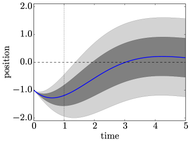
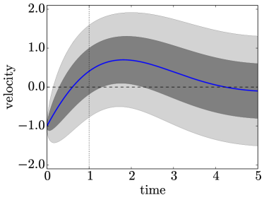
Figure 1: The position (left) and velocity (right) of a randomly forced harmonic oscillator with damping for $\omega_{0}=1=\lambda=\sigma$. The mean value is shown together with one (dark gray) and two standard deviations (light gray).

We first consider Eq. 1.5 with $d=1$ and

$$V(Q)=\frac{1}{2}\omega_{0}^{2}Q^{2}.$$ (5.1)

Physically, with this potential, Eq. 1.5 describes a randomly forced harmonic oscillator with resonance frequency $\omega_{0}$ and damping parameter $\lambda$; the strength of the Gaussian forcing is given by $\sigma$. For $\omega_{0}=0$ (i.e., in the absence of a potential), the SDE can be interpreted as a model for the dispersion of an atmospheric pollutant in a one-dimensional turbulent velocity field (see Rodean, (1996)). In this case, $\sigma^{2}/(2\lambda)$ is the turbulent-velocity variance and $1/\lambda$ the velocity relaxation-time. In Figure 1, the marginal distributions for the position and velocity are visualised as a function of $t$ for the first set of parameters used in the numerical experiments ($\omega_{0}=1=\lambda=\sigma$ and $P(0)=Q(0)=-1$).

We choose this simple example, for which we know the analytical solution, to verify the correctness of our code and to quantify numerical errors; exact solutions of the Langevin equation are also described in (Risken,, 1996). As the system is linear, the joint pdf of $Q$ and $P$ is Gaussian and is defined by their mean and covariance. Denoting ${\boldsymbol{X}}(t)=(Q(t),P(t))^{\mathsf{T}}$ and the initial solution by ${\boldsymbol{X}}_{0}={\boldsymbol{X}}(t=0)=(Q(t=0),P(t=0))^{\mathsf{T}}$, we have

$${\boldsymbol{X}}(t)=\exp\left[\mathchoice{\raisebox{0.0pt}{$\displaystyle{\vphantom{\bigm{|}}\mathopen{}-\Lambda t}$}}{-\Lambda t}{-\Lambda t}{-\Lambda t}\right]{\boldsymbol{X}}_{0}+\int_{0}^{t}\exp\left[\mathchoice{\raisebox{0.0pt}{$\displaystyle{\vphantom{\bigm{|}}\mathopen{}-\Lambda(t-s)}$}}{-\Lambda(t-s)}{-\Lambda(t-s)}{-\Lambda(t-s)}\right]{\boldsymbol{\Sigma}}\,dW(s)$$ (5.2)

with

$$\Lambda\coloneq\begin{pmatrix}0&-1\\ \omega_{0}^{2}&\lambda\end{pmatrix},\qquad{\boldsymbol{\Sigma}}\coloneq\begin{pmatrix}0\\ \sigma\end{pmatrix}.$$

${\boldsymbol{X}}(t)$ follows a Gaussian distribution with mean

$$\mathbb{E}\left[\mathchoice{\raisebox{0.0pt}{$\displaystyle{\vphantom{\bigm{|}}\mathopen{}{\boldsymbol{X}}(t)}$}}{{\boldsymbol{X}}(t)}{{\boldsymbol{X}}(t)}{{\boldsymbol{X}}(t)}\right]=\exp\left[\mathchoice{\raisebox{0.0pt}{$\displaystyle{\vphantom{\bigm{|}}\mathopen{}-\Lambda t}$}}{-\Lambda t}{-\Lambda t}{-\Lambda t}\right]{\boldsymbol{X}}_{0}$$ (5.3)

and covariance matrix

$$B(t)\coloneq\int_{0}^{t}\exp\left[\mathchoice{\raisebox{0.0pt}{$\displaystyle{\vphantom{\bigm{|}}\mathopen{}-\Lambda(t-s)}$}}{-\Lambda(t-s)}{-\Lambda(t-s)}{-\Lambda(t-s)}\right]{\boldsymbol{\Sigma}}{\boldsymbol{\Sigma}}^{\mathsf{T}}\exp\left[\mathchoice{\raisebox{0.0pt}{$\displaystyle{\vphantom{\bigm{|}}\mathopen{}-\Lambda^{\mathsf{T}}(t-s)}$}}{-\Lambda^{\mathsf{T}}(t-s)}{-\Lambda^{\mathsf{T}}(t-s)}{-\Lambda^{\mathsf{T}}(t-s)}\right]\,ds\,,$$ (5.4)

which can easily be evaluated using a computer algebra system.

Numerical results

We compute $\mathbb{E}\left[\mathchoice{\raisebox{0.0pt}{$\displaystyle{\vphantom{\bigm{|}}\mathopen{}\phi({\boldsymbol{X}}(1))}$}}{\phi({\boldsymbol{X}}(1))}{\phi({\boldsymbol{X}}(1))}{\phi({\boldsymbol{X}}(1))}\right]$ for $\phi(Q,P)=\exp(-2(P-0.5)^{2})\sqrt{2/\pi}$ and the following set of parameters:

1. $\omega_{0}=1$, $\lambda=4$ and $\sigma=2$.

2. $\omega_{0}=1$, $\lambda=9$ and $\sigma=3$.

The initial position and velocity were set to $Q(t=0)=P(t=0)=-1$ in both cases. Errors are computed using the exact value computed from Eqs. 5.3 and 5.4. The exact values are $0.447904416997582$ and $0.418086875513087$, respectively. The CPU time scaled by $\epsilon^{-2}$ and the error (bias error plus one standard deviation) scaled by $\epsilon$ are plotted in Figures 3 and 3 against $\epsilon$. The scaling means we expect both graphs to be flat. We observe for both parameter sets that the integrators based on the exact OU process are the most efficient for small $\epsilon$. Even though SVGe uses a weak fourth-order accurate integrator, the complexity of MLMC cannot be reduced beyond $\mathcal{O}\left(\mathchoice{\raisebox{0.0pt}{$\displaystyle{\vphantom{\bigm{|}}\mathopen{}\epsilon^{-2}}$}}{\epsilon^{-2}}{\epsilon^{-2}}{\epsilon^{-2}}\right)$ and it is the same as for the other integrators. The improvements come by improving constants, in this case by about a factor 4 in comparison to EMG. For the second set of parameter values in Figure 3, the relaxation time is shorter and the noise is larger, and the improvement due to the splitting methods is even more pronounced (factor 10).

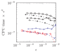
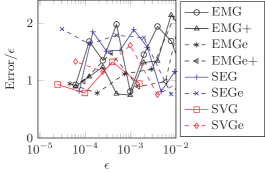
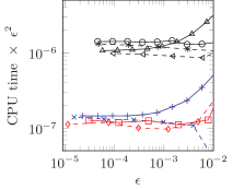
Figure 2: For the harmonic oscillator with parameter set 1. The left-hand plot shows the CPU time for a given value of $\epsilon$; the time is scaled by $\epsilon^{-2}$ and this leads to a nearly flat profile in each case. The right-hand plot shows the bias error plus one standard deviation; the errors are divided by $\epsilon$ to show both mean and standard deviation are $\mathcal{O}\left(\mathchoice{\raisebox{0.0pt}{$\displaystyle{\vphantom{\bigm{|}}\mathopen{}\epsilon}$}}{\epsilon}{\epsilon}{\epsilon}\right)$.

Figure 3: For the harmonic oscillator with parameter set 2. Compared to Figure 3, the difference between the splitting methods and Euler–Maruyama is significantly larger.

In order to take large time-steps, it is necessary to ensure the stability of the integrator. It is well known from deterministic differential equations that most explicit integrators will have a stability constraint on the time-step size. This is the same for SDEs and such stability constraints may severely restrict the number of levels that can be employed in the MLMC method and thus its efficiency (Hutzenthaler et al.,, 2013; Abdulle & Blumenthal,, 2013). Exact sampling of the Ornstein–Uhlenbeck process poses no stability constraints, allowing for smaller values of $M_{0}$ and thus for larger numbers of levels in MLMC in the case of splitting methods. For example, in the above simulations, increasing the number of time steps from $M_{0}=4$ to $M_{0}=8$ in Euler-Maruyama (cf. EMG and EMG+, as well as EMGe and EMGe+) lead to an improvement in efficiency. The same change has no effect in SEG. However, the symplectic methods we are using for the Hamiltonian part are explicit and have their own stability constraint (Skeel & Izaguirre,, 2002), somewhat limiting this benefit of splitting methods.

5.2 Double-well potential

We now change the potential and consider the double-well potential

$$V(Q)=\frac{\omega_{0}^{2}}{8Q_{\min}^{2}}(Q^{2}-Q_{\min}^{2})^{2},$$

where $Q_{\min}$ and $\omega_{0}$ are parameters. We compute $\mathbb{E}\left[\mathchoice{\raisebox{0.0pt}{$\displaystyle{\vphantom{\bigm{|}}\mathopen{}\phi({\boldsymbol{X}}(T))}$}}{\phi({\boldsymbol{X}}(T))}{\phi({\boldsymbol{X}}(T))}{\phi({\boldsymbol{X}}(T))}\right]$ for $\phi(Q,P)\coloneq(Q+Q_{\min})^{2}+P^{2}$ (note $(Q+Q_{\min})^{2}$ takes distinct values at the bottom of the wells $Q=\pm Q_{\min}$).

For the numerical experiments in Figure 5, we choose parameter values $Q_{\min}=\omega_{0}=1$, $\lambda=2$, $\sigma=4$, and take initial data $Q(t=0)=P(t=0)=-1$. The scaled CPU time and error for $T=1$ are plotted against $\epsilon$ in Figure 5, where errors are computed relative to a numerically computed value given by $4.52782626985$. It is noticeable again that the splitting methods and especially the symplectic Euler-based methods are most efficient.

In Figure 5, we explore the behaviour of the algorithm as we increase the length of the time interval $T$. For the plot, we scale the CPU time by $\epsilon^{-2}T$; the computation time scales linearly with the number of time steps and, by scaling by $T$, we see how the MLMC algorithm behaves with increasing $T$. The errors are computed relative to the numerically computed values $6.11075602345$ for $T=2$; $7.11570774835$ for $T=4$; and $7.2125872733$ for $T=8$. The values for $T=4$ and $T=8$ are close, which indicates the system has moved close to the invariant measure by this time. In each case, SEG is most efficient and we see the measure of CPU time $\times\epsilon^{2}/T$ decrease from about $5\times 10^{-5}$ for $T=1$ to about $10^{-4}$ for $T=8$. The profiles are also less flat as $T$ is increased, indicating that the time steps may not be small enough to have entered the asymptotic regime. It is natural that the gains become less pronounced, when we come close to the invariant measure and the coupling between levels has decayed.

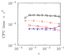
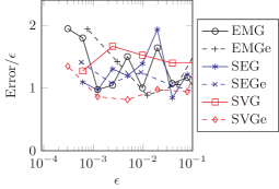
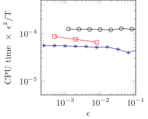
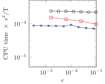
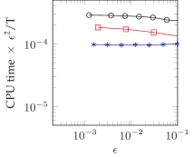
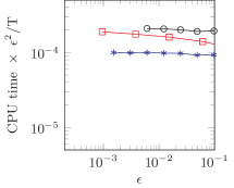
Figure 4: Numerical results for the double-well potential (plots as above).

Figure 5: From top-left to bottom-right, plots of CPU time scaled by $T\epsilon^{-2}$ for $T=1,2,4,8$ and the double-well potential with $\omega_{0}=1$, $\lambda=2$, $\sigma=4$.

6 Further enhancements

Theorems 3.4 and 3.2 provide a route to analysing the MLMC entirely by weak-approximation properties of the numerical method. This has a number of advantages: from the theoretical point of view, the analysis works for a wider set of test functions compared to the analysis of (Giles,, 2008), which demands that quantities of interest $\phi$ are globally Lipschitz continuous. From the algorithmic point of view, the order of weak convergence is determined by moment conditions up to a given degree depending on the order of convergence. There are a number of ways to satisfy these conditions. It is widely known (Kloeden & Platen,, 1992) that the Gaussian random variables can be replaced by discrete random variables without disturbing the weak order of convergence. The obvious question then is whether we can use discrete random variables to our advantage also in the context of MLMC.

MLMC depends crucially on the fact that the sum of two independent Gaussian random variables is also Gaussian. This allows increments to be generated on the fine levels and combined to give a random variable with the same distribution on the next coarser level, using Eq. 4.9. Discrete variables do not have this property. While Theorem 3.4 implies the coupling condition of Theorem 2.1(iii), the sum of two three-point random variables is not a three-point random variable and the telescoping sum breaks down. In general, using discrete random variables with MLMC introduces extra error due to the telescoping sum no longer being exact. Though (Belomestny & Nagapetyan,, 2014) provides an approach that preserves the telescoping sum by using a different discrete random variable on each level. Here we do not follow this route. Instead, we use the same discrete random variable on each level, accepting the additional bias error that this introduces, which crucially is of higher order. To control this additional bias and to ensure the total error is still below our chosen tolerance, we change the number of levels $L$ and the coarsest mesh size $h_{0}$. Discrete random variables are cheaper to generate than Gaussian random variables and the coarsest level can be evaluated exactly, which we exploit to achieve a significant speed-up in the small noise case.

6.1 Random variables with discrete distribution

The modified equations are unchanged if the Gaussian random variables in the integrator are replaced by random variables with the same moments to order five (including all cross moments to order five arising from the doubled-up system). For example, we can replace samples of iid $\operatorname{N}(0,1)$ random variables by iid samples of the random variable $\zeta$ with distribution

$$\mathbb{P}\left(\mathchoice{\raisebox{0.0pt}{$\displaystyle{\vphantom{\bigm{|}}\mathopen{}\zeta=0}$}}{\zeta=0}{\zeta=0}{\zeta=0}\right)=\frac{2}{3},\qquad\mathbb{P}\left(\mathchoice{\raisebox{0.0pt}{$\displaystyle{\vphantom{\bigm{|}}\mathopen{}\zeta=\pm\sqrt{3}}$}}{\zeta=\pm\sqrt{3}}{\zeta=\pm\sqrt{3}}{\zeta=\pm\sqrt{3}}\right)=\frac{1}{6};$$ (6.1)

or

$$\mathbb{P}\left(\mathchoice{\raisebox{0.0pt}{$\displaystyle{\vphantom{\bigm{|}}\mathopen{}\zeta=\pm\sqrt{3+\sqrt{6}}}$}}{\zeta=\pm\sqrt{3+\sqrt{6}}}{\zeta=\pm\sqrt{3+\sqrt{6}}}{\zeta=\pm\sqrt{3+\sqrt{6}}}\right)=c,\qquad\mathbb{P}\left(\mathchoice{\raisebox{0.0pt}{$\displaystyle{\vphantom{\bigm{|}}\mathopen{}\zeta=\pm\sqrt{3-\sqrt{6}}}$}}{\zeta=\pm\sqrt{3-\sqrt{6}}}{\zeta=\pm\sqrt{3-\sqrt{6}}}{\zeta=\pm\sqrt{3-\sqrt{6}}}\right)=\frac{1}{2}-c,\qquad c\coloneq\frac{1}{2}\left(\mathchoice{\raisebox{0.0pt}{$\displaystyle{\vphantom{\bigm{|}}\mathopen{}1-\frac{3+\sqrt{6}}{6}}$}}{1-\frac{3+\sqrt{6}}{6}}{1-\frac{3+\sqrt{6}}{6}}{1-\frac{3+\sqrt{6}}{6}}\right).$$ (6.2)

We refer to $\zeta$ as the three- and four-point approximations to the Gaussian, respectively. This is a well-known trick for weak approximation of SDEs, e.g. (Kloeden & Platen,, 1992, §14.2). The approximations have a number of advantages, as $\zeta$ is quicker to sample than a Gaussian and, due to the finite number of states, averages of functionals of $\zeta$ can be computed exactly.

6.2 Exact evaluation of the coarse-level expectation

For all our integrators, the evaluation of the coarse-level estimator $\widehat{\mathcal{P}}_{0}$ with time step $h_{0}=T/M_{0}$ is the computationally most expensive part of the MLMC algorithm: even though the number of time steps and hence the number of samples per path is small, a large number of individual paths needs to be evaluated to reduce the variance of the coarse-level estimator. This cost can be reduced dramatically if a discrete distribution as discussed in Section 6.1 is used for the individual samples ${\boldsymbol{\xi}}_{n}$. In this case, a significantly cheaper estimator, which does not rely on Monte Carlo sampling, can be constructed. If the random numbers ${\boldsymbol{\xi}}_{1},\dots,{\boldsymbol{\xi}}_{M_{0}}$ for each path are drawn from the three-point approximation in Eq. 6.1, there is only a finite number $n_{{\boldsymbol{\xi}}}$ of possible samples ${\boldsymbol{\xi}}^{(i)}=\{{\boldsymbol{\xi}}^{(i)}_{1},\dots,{\boldsymbol{\xi}}^{(i)}_{M_{0}}\}$, each with associated probability $\mathbb{P}({\boldsymbol{\xi}}^{(i)})=\mathbb{P}({\boldsymbol{\xi}}_{1}={\boldsymbol{\xi}}_{1}^{(i)})\cdots\mathbb{P}({\boldsymbol{\xi}}_{M_{0}}={\boldsymbol{\xi}}_{M_{0}}^{(i)})$. The expectation value of the quantity of interest can be calculated exactly on the coarsest level as

$$\widehat{Y}_{0}^{\operatorname{exact}}=\widehat{\mathcal{P}}^{\operatorname{exact}}_{0}=\sum_{i=1}^{n_{{\boldsymbol{\xi}}}}\mathbb{P}({\boldsymbol{\xi}}={\boldsymbol{{\boldsymbol{\xi}}}}^{(i)})\mathcal{P}_{0}^{(i)}.$$ (6.3)

For the three-point approximation, for example, we need to choose from the $3^{d}$ possible values of ${\boldsymbol{\xi}}_{n}$ in each of the $M_{0}$ time steps, so $n_{{\boldsymbol{\xi}}}=(3^{d})^{M_{0}}$ is the number of different samples of ${\boldsymbol{\xi}}$. Since the estimator contains no sampling error, its variance is zero. In Algorithm 1, we can replace $\widehat{Y}_{0,N_{0}}\mapsto\widehat{Y}_{0}^{\operatorname{exact}}$ and $\widehat{V}_{0,N_{0}}\mapsto 0$ in lines 10 and 12. Effectively, this implies that the sum in line 12 only runs from $j=1$ to $L$ and it is not necessary to evaluate $N_{0}^{+}$.

Naively, the computational complexity of evaluating Eq. 6.3 is given by the product of the number of different samples and the number of time steps, $n_{{\boldsymbol{\xi}}}\times M_{0}=M_{0}(3^{dM_{0}})$. However, using a recursive algorithm, the computational complexity can be reduced to the number of nodes in the product-probability tree, which is only $\mathcal{O}\left(\mathchoice{\raisebox{0.0pt}{$\displaystyle{\vphantom{\bigm{|}}\mathopen{}n_{{\boldsymbol{\xi}}}}$}}{n_{{\boldsymbol{\xi}}}}{n_{{\boldsymbol{\xi}}}}{n_{{\boldsymbol{\xi}}}}\right)=\mathcal{O}(3^{dM_{0}})$ Nevertheless, this still grows exponentially with the number $M_{0}$ of coarse time steps and so Eq. 6.3 is only competitive for small values of $M_{0}$ and $d$. However, exact evaluation can reduce the overall cost of the algorithm dramatically and this is exploited to significant advantage in Section 6.3.

We now state and prove a modified complexity theorem that allows for additional bias to be introduced between levels, as well as for a different computational cost on the coarsest level.

Let $\widetilde{\mathcal{P}}_{\ell}$ be the estimator corresponding to $\widehat{\mathcal{P}}_{\ell}$, but with increments given by Eq. 4.9. For Gaussian increments these estimators are the same, but they are different when we use 3-point or 4-point approximations. Recall that the fine, level $\ell$, sample in each of the estimators $\widehat{Y}_{\ell,N_{\ell}}$ uses increments sampled directly from the 3-point or 4-point distribution, while the coarse, level $\ell-1$, sample is computed using two consecutive fine increments and formula Eq. 4.9.

Theorem 6.1.

Let us replace Assumption (ii) of Theorem 2.1 by

1. $\mathbb{E}\left[\mathchoice{\raisebox{0.0pt}{$\displaystyle{\vphantom{\bigm{|}}\mathopen{}\widehat{Y}_{0}}$}}{\widehat{Y}_{0}}{\widehat{Y}_{0}}{\widehat{Y}_{0}}\right]=\mathbb{E}\left[\mathchoice{\raisebox{0.0pt}{$\displaystyle{\vphantom{\bigm{|}}\mathopen{}\widehat{\mathcal{P}}_{\ell}}$}}{\widehat{\mathcal{P}}_{\ell}}{\widehat{\mathcal{P}}_{\ell}}{\widehat{\mathcal{P}}_{\ell}}\right]$  and  $\left|\mathbb{E}\left[\mathchoice{\raisebox{0.0pt}{$\displaystyle{\vphantom{\bigm{|}}\mathopen{}\widehat{\mathcal{P}}_{\ell}-\widetilde{\mathcal{P}}_{\ell}}$}}{\widehat{\mathcal{P}}_{\ell}-\widetilde{\mathcal{P}}_{\ell}}{\widehat{\mathcal{P}}_{\ell}-\widetilde{\mathcal{P}}_{\ell}}{\widehat{\mathcal{P}}_{\ell}-\widetilde{\mathcal{P}}_{\ell}}\right]\right|\leq c_{0}h_{\ell}^{\gamma}$,

for some positive constants $c_{0}$ and $\gamma>\alpha\geq\frac{1}{2}$. We suppose that all the other assumptions of Theorem 2.1 hold, except that $\mathrm{Cost}^{(\operatorname{MLMC})}_{0}$ is not necessarily assumed to be bounded by $c_{3}N_{0}h_{0}^{-1}$ any longer. Then, there exists a positive constant $c_{5}$ such that for any $\epsilon<1/e$, there are values $M_{0}$, $L$ and $N_{\ell}$ for which $\widehat{Y}_{\{N_{\ell}\}}$ from Eq. 2.2 has a MSE $<\epsilon^{2}$ and a computational complexity $\mathrm{Cost}^{(\operatorname{MLMC})}$ with bound

$$\mathrm{Cost}^{(\operatorname{MLMC})}\leq\mathrm{Cost}^{(\operatorname{MLMC})}_{0}+c_{5}\epsilon^{-2+1/\gamma}\,.$$ (6.4)

Proof.

We only require slight modifications in the proof of (Giles,, 2008, Theorem 3.1) to prove this result. In particular, it is sufficient to choose

$$L=\left\lceil\frac{\log_{2}(\sqrt{3}c_{1}T^{\alpha}\epsilon^{-1})}{\alpha}\right\rceil$$

to bound the bias on the finest level. The factor $\sqrt{3}$ appears, since we now have three error contributions, the bias on the finest level, the bias between levels and the sampling error, and since we require each of these contributions to the MSE to be less than $\epsilon^{2}/3$.

To guarantee that the bias between levels is less than $\epsilon^{2}/3$, note that due to assumption (ii) we have

$$\left|\sum_{\ell=0}^{L-1}\mathbb{E}\left[\mathchoice{\raisebox{0.0pt}{$\displaystyle{\vphantom{\bigm{|}}\mathopen{}\widehat{\mathcal{P}}_{\ell}-\widetilde{\mathcal{P}}_{\ell}}$}}{\widehat{\mathcal{P}}_{\ell}-\widetilde{\mathcal{P}}_{\ell}}{\widehat{\mathcal{P}}_{\ell}-\widetilde{\mathcal{P}}_{\ell}}{\widehat{\mathcal{P}}_{\ell}-\widetilde{\mathcal{P}}_{\ell}}\right]\right|\leq\sum_{\ell=0}^{L-1}\left|\mathbb{E}\left[\mathchoice{\raisebox{0.0pt}{$\displaystyle{\vphantom{\bigm{|}}\mathopen{}\widehat{\mathcal{P}}_{\ell}-\widetilde{\mathcal{P}}_{\ell}}$}}{\widehat{\mathcal{P}}_{\ell}-\widetilde{\mathcal{P}}_{\ell}}{\widehat{\mathcal{P}}_{\ell}-\widetilde{\mathcal{P}}_{\ell}}{\widehat{\mathcal{P}}_{\ell}-\widetilde{\mathcal{P}}_{\ell}}\right]\right|\leq c_{0}h_{0}^{\gamma}\sum_{\ell=0}^{L-1}2^{-\ell\gamma}<\frac{\sqrt{2}c_{0}}{\sqrt{2}-1}\,h_{0}^{\gamma}\,,$$

and so a sufficient condition is $h_{0}\leq c_{6}\epsilon^{1/\gamma}$ with $c_{6}=\left(\frac{\sqrt{3}}{c_{0}}\left(1-\frac{1}{\sqrt{2}}\right)\right)^{1/\gamma}$ .

Finally, setting

$$N_{\ell}=\left\lceil\frac{3c_{2}h_{0}^{2}}{\sqrt{2}-1}\epsilon^{-2}2^{-3\ell/2}\right\rceil$$

and exploiting standard results about geometric series, we get

$$\sum_{\ell=1}^{L}\operatorname{Var}\left[\mathchoice{\raisebox{0.0pt}{$\displaystyle{\vphantom{\bigm{|}}\mathopen{}\widehat{Y}_{\ell,N_{\ell}}}$}}{\widehat{Y}_{\ell,N_{\ell}}}{\widehat{Y}_{\ell,N_{\ell}}}{\widehat{Y}_{\ell,N_{\ell}}}\right]\leq\frac{\epsilon^{2}}{3}\left(\sqrt{2}-1\right)\sum_{\ell=1}^{L}\frac{c_{2}h_{\ell}^{2}}{c_{2}h_{0}^{2}}2^{3\ell/2}\leq\frac{\epsilon^{2}}{3}\left(\sqrt{2}-1\right)\sum_{\ell=1}^{L}2^{-\ell/2}\leq\frac{\epsilon^{2}}{3}\,.$$

The computational cost can then be bounded by

$$\mathrm{Cost}^{(\operatorname{MLMC})}\leq\mathrm{Cost}^{(\operatorname{MLMC})}_{0}+c_{3}\sum_{\ell=1}^{L}N_{\ell}h_{\ell}^{-1}\leq\mathrm{Cost}^{(\operatorname{MLMC})}_{0}+\frac{3c_{2}c_{3}h_{0}}{\sqrt{2}-1}\epsilon^{-2}\sum_{\ell=1}^{L}2^{-\ell/2}$$

which leads to the desired bound with $c_{5}=3c_{2}c_{3}c_{6}\left(\sqrt{2}-1\right)^{-2}$. (Note that as in (Giles,, 2008) this (optimal) choice of $N_{\ell}$ is obtained by minimising the cost on levels 1 to $L$ subject to the constraint that the sum of the variances is less than $\epsilon^{2}/3$.) ∎

If we use a $q$-point approximation and the expected value on the coarsest level is computed excactly, as described in Section 6.2, then $\mathrm{Cost}^{(\operatorname{MLMC})}_{0}=\mathcal{O}(q^{dM_{0}})=\mathcal{O}\Big{(}\eta^{\epsilon^{-{1}/{\gamma}}}\Big{)}$, for some $\eta>1$. Hence, the total cost grows exponentially with $\epsilon$, as expected. However, for practically relevant values of $\epsilon$, the exponential term may not be dominant and we may get significant computational savings, as we will see in the next section. Note that $\gamma=2$ for the three-point and $\gamma=3$ for the four-point case, leading to a cost of $\mathcal{O}(\epsilon^{-3/2})$ and $\mathcal{O}(\epsilon^{-5/3})$ for the computation of the correction terms on levels 1 to $L$, respectively.

Since the sampling of discrete random variables is significantly cheaper, it may also be of interest to use standard Monte Carlo on the coarsest level, as in the earlier sections of this paper. If we slightly increase the constant in the formula for $N_{\ell}$, $\ell=1,\ldots,L$, in the proof of Theorem 6.1 and choose $N_{0}=\mathcal{O}(\epsilon^{-2})$ such that the total variance over all levels is below $\epsilon^{2}/3$, then the dominant cost will be $\mathrm{Cost}^{(\operatorname{MLMC})}_{0}=\mathcal{O}(N_{0}h_{0}^{-1})$, and so $\mathrm{Cost}^{(\operatorname{MLMC})}\leq c_{5}^{*}\epsilon^{-2-1/\gamma}$, which will be $\mathcal{O}(\epsilon^{-5/2})$ and $\mathcal{O}(\epsilon^{-7/3})$ in the three- and four-point cases, respectively. However, in practice $c_{5}^{*}$ is significantly smaller than the constant $c_{4}$ in Theorem 2.1, so that for moderate values of $\epsilon$, the use of discrete random variables will pay off.

6.3 Numerical experiments with discrete random variables

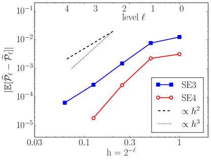
Figure 6: $h$-dependency of the additional bias term $|\mathbb{E}\left[\mathchoice{\raisebox{0.0pt}{$\displaystyle{\vphantom{\bigm{|}}\mathopen{}\widehat{\mathcal{P}}_{\ell}-\widetilde{\mathcal{P}}_{\ell}}$}}{\widehat{\mathcal{P}}_{\ell}-\widetilde{\mathcal{P}}_{\ell}}{\widehat{\mathcal{P}}_{\ell}-\widetilde{\mathcal{P}}_{\ell}}{\widehat{\mathcal{P}}_{\ell}-\widetilde{\mathcal{P}}_{\ell}}\right]|$ (see (ii) in Theorem 6.1) for $\sigma_{0}=\lambda=1$, $\sigma=0.4$ computed using the symplectic Euler/exact OU splitting. Results are shown both for three-point (SE3) and four-point (SE4) random variables.

We carry out numerical experiments as in Section 5.1 with the damped harmonic oscillator, but change the parameters slightly to $\omega_{0}=\lambda=1$, $\sigma=0.4$ (i.e., smaller noise). Instead of sampling from a Gaussian distribution, we use discrete random numbers, which introduce an additional bias as discussed above. To quantify this bias numerically, we plot the difference $\left|\mathbb{E}\left[\mathchoice{\raisebox{0.0pt}{$\displaystyle{\vphantom{\bigm{|}}\mathopen{}\widehat{\mathcal{P}}_{\ell}-\widetilde{\mathcal{P}}_{\ell}}$}}{\widehat{\mathcal{P}}_{\ell}-\widetilde{\mathcal{P}}_{\ell}}{\widehat{\mathcal{P}}_{\ell}-\widetilde{\mathcal{P}}_{\ell}}{\widehat{\mathcal{P}}_{\ell}-\widetilde{\mathcal{P}}_{\ell}}\right]\right|$ in Figure 6 for the symplectic Euler/exact OU method both for three-point (SE3) and four point (SE4) distributions. The figure shows that, as predicted in Kloeden et al., (1995), the additional bias is proportional to $h^{2}$ for SE3 and to $h^{3}$ for SE4. We have also studied the dependence on the noise term (not shown here) and found that, as $\sigma$ gets smaller, the additional bias is reduced very rapidly (proportional to $\sigma^{3}$ and $\sigma^{4}$, respectively).

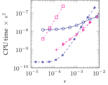
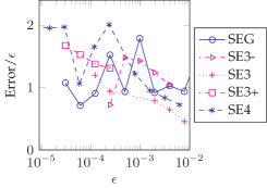
Figure 7: Harmonic oscillator with $\lambda=1$ and $\sigma=0.4$ computed using the symplectic Euler/exact OU splitting method using three-point (SE3-, SE3, SE3+) and four-point (SE4) random variables.

For the same setup, we measure the computational cost and the total error (consisting of the statistical error, discretisation error and the additional bias introduced by sampling from discrete distributions). We calculate the same quantity of interest as in Section 5.1. Figure 7 shows the results both for Gaussian random variables (SEG) and for the three- and four-point distributions (SE3 and SE4) with $M_{0}=8$. For the discrete distributions, the coarse-grid expectation value is calculated exactly. For the three-point distribution, we also varied the number of time steps on the coarsest level and use $M_{0}=4$ (SE3-), $M_{0}=8$ (SE3) and $M_{0}=16$ (SE3+). In each case, we only show results up to the point where the additional bias error becomes too large. For fixed $\epsilon$, the SE3+ method is more expensive than SE3 and SE3-, since the cost of the exact coarse-level evaluation grows exponentially with the number of time steps. On the other hand, using smaller time steps on the coarsest level allows the use of this method for smaller values $\epsilon$ where the additional bias becomes too large for SE3- and SE3. The additional bias in the SE4 method is so small that the method can be used up to values as small as $\epsilon=10^{-5}$. Comparing the cost of this method to the Gaussian case shows that using a discrete four-point distribution is more than 50-times faster in this case.

We conclude that, if used with caution, approximating the Gaussian increments in Eq. 1.2 by discrete approximations and calculating the coarse-level expectation value exactly can significantly improve the efficiency of the multilevel method.

7 Conclusion

Table 1 summarises our findings: MLMC gives a significant speed-up over the traditional Monte Carlo computation of averages and, even though the optimal complexity estimate $\mathcal{O}\left(\mathchoice{\raisebox{0.0pt}{$\displaystyle{\vphantom{\bigm{|}}\mathopen{}\epsilon^{-2}}$}}{\epsilon^{-2}}{\epsilon^{-2}}{\epsilon^{-2}}\right)$ for Monte Carlo-type methods holds for all the integrators under study, there is significant variation between the integrators. Splitting methods are particularly appropriate for the Langevin equation and using the exact OU solution yields a more stable integrator than Euler–Maruyama, even though both integrators are explicit. In the experiments, the difference in computation time between Euler–Maruyama and the splitting methods is greater when the dissipation $\lambda$ is higher, since Euler–Maruyama suffers from a more severe time-step restriction (cf. Figures 3–5).

	Harmonic Oscillator (Set 2)		Double-well Potential
	$\epsilon=2.4\times 10^{-4}$	ratio	$\epsilon=2.44\times 10^{-3}$	ratio
MC w. EMG	467 sec	13$\times$ slower	1710 sec	378$\times$ slower
MLMC w. EMG	33.8 sec	1	45.2 sec	1
MLMC w. SEGe	2.15 sec	15$\times$ faster	10.5 sec	4.3$\times$ faster

Table 1: Comparison of Monte Carlo with Euler–Maruyama, MLMC with Euler–Maruyama and MLMC with the symplectic Euler/OU integrator and extrapolation (using Gaussian increments).

This paper also introduced an alternative analysis method for MLMC based on modified equations. It provides a convenient approach to MLMC through weak-approximation theory; strong-approximation theory is only needed to relate the original and modified equations and not the numerical methods. This accommodated the use of the splitting method and the exact OU solution easily.

The weak-approximation analysis motivated the use of discrete random variables, such as three- and four-point approximations to the Gaussian. In an example with small noise ($\sigma=0.4$ and $\lambda=1$), we saw between one and two orders of magnitude speed-up for a useful range of $\epsilon$ because we can evaluate the coarse level exactly. This method is easy to implement and it works well because the dominant cost lies on the coarsest level for these problems. While the speed improvements are impressive, this method should be used with care as it introduces an extra bias error. The extra bias can be estimated as shown in Figure 6. The improvement would be less dramatic in higher dimensions as the number of samples required would increase dramatically and it may be impossible to compute the coarse level exactly. As an interesting side result, we proved a modified complexity theorem that allows for extra bias to be introduced between levels in MLMC.

Appendix A Proof of Lemma 3.3

Proof.

This is a standard Gronwall argument with the Ito isometry. The integral equation for the difference ${\boldsymbol{X}}(t)-{\boldsymbol{X}}_{h}(t)$ is

$${\boldsymbol{X}}(t)-{\boldsymbol{X}}_{h}(t) =\int_{0}^{t}\left(\mathchoice{\raisebox{0.0pt}{$\displaystyle{\vphantom{\bigm{|}}\mathopen{}{\boldsymbol{f}}({\boldsymbol{X}}(s))-{\tilde{{\boldsymbol{f}}\mkern 4.0mu}\mkern-4.0mu}{}({\boldsymbol{X}}_{h}(s))}$}}{{\boldsymbol{f}}({\boldsymbol{X}}(s))-{\tilde{{\boldsymbol{f}}\mkern 4.0mu}\mkern-4.0mu}{}({\boldsymbol{X}}_{h}(s))}{{\boldsymbol{f}}({\boldsymbol{X}}(s))-{\tilde{{\boldsymbol{f}}\mkern 4.0mu}\mkern-4.0mu}{}({\boldsymbol{X}}_{h}(s))}{{\boldsymbol{f}}({\boldsymbol{X}}(s))-{\tilde{{\boldsymbol{f}}\mkern 4.0mu}\mkern-4.0mu}{}({\boldsymbol{X}}_{h}(s))}\right)\,ds$$

$$\quad+\int_{0}^{t}\left(\mathchoice{\raisebox{0.0pt}{$\displaystyle{\vphantom{\bigm{|}}\mathopen{}G({\boldsymbol{X}}(s))-\widetilde{G}({\boldsymbol{X}}_{h}(s))}$}}{G({\boldsymbol{X}}(s))-\widetilde{G}({\boldsymbol{X}}_{h}(s))}{G({\boldsymbol{X}}(s))-\widetilde{G}({\boldsymbol{X}}_{h}(s))}{G({\boldsymbol{X}}(s))-\widetilde{G}({\boldsymbol{X}}_{h}(s))}\right)\,d{\boldsymbol{W}}(s),$$

where ${\tilde{{\boldsymbol{f}}\mkern 4.0mu}\mkern-4.0mu}{}\coloneq{\boldsymbol{f}}+h{\boldsymbol{f}}_{1}$ and $\widetilde{G}\coloneq G+hG_{1}$. By conditions (i) and (ii),

$$\left\|\mathchoice{\raisebox{0.0pt}{$\displaystyle{\vphantom{\bigm{|}}\mathopen{}{\boldsymbol{f}}({\boldsymbol{X}}(s))-{\boldsymbol{f}}({\boldsymbol{X}}_{h}(s))-h{\boldsymbol{f}}_{1}({\boldsymbol{X}}_{h}(s))}$}}{\smash{{\boldsymbol{f}}({\boldsymbol{X}}(s))-{\boldsymbol{f}}({\boldsymbol{X}}_{h}(s))-h{\boldsymbol{f}}_{1}({\boldsymbol{X}}_{h}(s))}}{{\boldsymbol{f}}({\boldsymbol{X}}(s))-{\boldsymbol{f}}({\boldsymbol{X}}_{h}(s))-h{\boldsymbol{f}}_{1}({\boldsymbol{X}}_{h}(s))}{{\boldsymbol{f}}({\boldsymbol{X}}(s))-{\boldsymbol{f}}({\boldsymbol{X}}_{h}(s))-h{\boldsymbol{f}}_{1}({\boldsymbol{X}}_{h}(s))}\right\|_{L^{2}(\Omega,{}^{d})}\leq L\left\|\mathchoice{\raisebox{0.0pt}{$\displaystyle{\vphantom{\bigm{|}}\mathopen{}{\boldsymbol{X}}(s)-{\boldsymbol{X}}_{h}(s)}$}}{\smash{{\boldsymbol{X}}(s)-{\boldsymbol{X}}_{h}(s)}}{{\boldsymbol{X}}(s)-{\boldsymbol{X}}_{h}(s)}{{\boldsymbol{X}}(s)-{\boldsymbol{X}}_{h}(s)}\right\|_{L^{2}(\Omega,{}^{d})}+C_{1}h$$

and similarly for $G$. Assume ${\boldsymbol{X}}(0)={\boldsymbol{X}}_{h}(0)$. The Ito isometry and Jensen’s inequality give

$$\mathbb{E}\left[\mathchoice{\raisebox{0.0pt}{$\displaystyle{\vphantom{\bigm{|}}\mathopen{}\left\|\mathchoice{\raisebox{0.0pt}{$\displaystyle{\vphantom{\bigm{|}}\mathopen{}{\boldsymbol{X}}(t)-{\boldsymbol{X}}_{h}(t)}$}}{\smash{{\boldsymbol{X}}(t)-{\boldsymbol{X}}_{h}(t)}}{{\boldsymbol{X}}(t)-{\boldsymbol{X}}_{h}(t)}{{\boldsymbol{X}}(t)-{\boldsymbol{X}}_{h}(t)}\right\|^{2}}$}}{\left\|\mathchoice{\raisebox{0.0pt}{$\displaystyle{\vphantom{\bigm{|}}\mathopen{}{\boldsymbol{X}}(t)-{\boldsymbol{X}}_{h}(t)}$}}{\smash{{\boldsymbol{X}}(t)-{\boldsymbol{X}}_{h}(t)}}{{\boldsymbol{X}}(t)-{\boldsymbol{X}}_{h}(t)}{{\boldsymbol{X}}(t)-{\boldsymbol{X}}_{h}(t)}\right\|^{2}}{\left\|\mathchoice{\raisebox{0.0pt}{$\displaystyle{\vphantom{\bigm{|}}\mathopen{}{\boldsymbol{X}}(t)-{\boldsymbol{X}}_{h}(t)}$}}{\smash{{\boldsymbol{X}}(t)-{\boldsymbol{X}}_{h}(t)}}{{\boldsymbol{X}}(t)-{\boldsymbol{X}}_{h}(t)}{{\boldsymbol{X}}(t)-{\boldsymbol{X}}_{h}(t)}\right\|^{2}}{\left\|\mathchoice{\raisebox{0.0pt}{$\displaystyle{\vphantom{\bigm{|}}\mathopen{}{\boldsymbol{X}}(t)-{\boldsymbol{X}}_{h}(t)}$}}{\smash{{\boldsymbol{X}}(t)-{\boldsymbol{X}}_{h}(t)}}{{\boldsymbol{X}}(t)-{\boldsymbol{X}}_{h}(t)}{{\boldsymbol{X}}(t)-{\boldsymbol{X}}_{h}(t)}\right\|^{2}}\right]\leq 2t\int_{0}^{t}\mathbb{E}\left[\mathchoice{\raisebox{0.0pt}{$\displaystyle{\vphantom{\bigm{|}}\mathopen{}\left\|\mathchoice{\raisebox{0.0pt}{$\displaystyle{\vphantom{\bigm{|}}\mathopen{}{\boldsymbol{f}}({\boldsymbol{X}}(s))-{\tilde{{\boldsymbol{f}}\mkern 4.0mu}\mkern-4.0mu}{}({\boldsymbol{X}}_{h}(s))}$}}{\smash{{\boldsymbol{f}}({\boldsymbol{X}}(s))-{\tilde{{\boldsymbol{f}}\mkern 4.0mu}\mkern-4.0mu}{}({\boldsymbol{X}}_{h}(s))}}{{\boldsymbol{f}}({\boldsymbol{X}}(s))-{\tilde{{\boldsymbol{f}}\mkern 4.0mu}\mkern-4.0mu}{}({\boldsymbol{X}}_{h}(s))}{{\boldsymbol{f}}({\boldsymbol{X}}(s))-{\tilde{{\boldsymbol{f}}\mkern 4.0mu}\mkern-4.0mu}{}({\boldsymbol{X}}_{h}(s))}\right\|^{2}}$}}{\left\|\mathchoice{\raisebox{0.0pt}{$\displaystyle{\vphantom{\bigm{|}}\mathopen{}{\boldsymbol{f}}({\boldsymbol{X}}(s))-{\tilde{{\boldsymbol{f}}\mkern 4.0mu}\mkern-4.0mu}{}({\boldsymbol{X}}_{h}(s))}$}}{\smash{{\boldsymbol{f}}({\boldsymbol{X}}(s))-{\tilde{{\boldsymbol{f}}\mkern 4.0mu}\mkern-4.0mu}{}({\boldsymbol{X}}_{h}(s))}}{{\boldsymbol{f}}({\boldsymbol{X}}(s))-{\tilde{{\boldsymbol{f}}\mkern 4.0mu}\mkern-4.0mu}{}({\boldsymbol{X}}_{h}(s))}{{\boldsymbol{f}}({\boldsymbol{X}}(s))-{\tilde{{\boldsymbol{f}}\mkern 4.0mu}\mkern-4.0mu}{}({\boldsymbol{X}}_{h}(s))}\right\|^{2}}{\left\|\mathchoice{\raisebox{0.0pt}{$\displaystyle{\vphantom{\bigm{|}}\mathopen{}{\boldsymbol{f}}({\boldsymbol{X}}(s))-{\tilde{{\boldsymbol{f}}\mkern 4.0mu}\mkern-4.0mu}{}({\boldsymbol{X}}_{h}(s))}$}}{\smash{{\boldsymbol{f}}({\boldsymbol{X}}(s))-{\tilde{{\boldsymbol{f}}\mkern 4.0mu}\mkern-4.0mu}{}({\boldsymbol{X}}_{h}(s))}}{{\boldsymbol{f}}({\boldsymbol{X}}(s))-{\tilde{{\boldsymbol{f}}\mkern 4.0mu}\mkern-4.0mu}{}({\boldsymbol{X}}_{h}(s))}{{\boldsymbol{f}}({\boldsymbol{X}}(s))-{\tilde{{\boldsymbol{f}}\mkern 4.0mu}\mkern-4.0mu}{}({\boldsymbol{X}}_{h}(s))}\right\|^{2}}{\left\|\mathchoice{\raisebox{0.0pt}{$\displaystyle{\vphantom{\bigm{|}}\mathopen{}{\boldsymbol{f}}({\boldsymbol{X}}(s))-{\tilde{{\boldsymbol{f}}\mkern 4.0mu}\mkern-4.0mu}{}({\boldsymbol{X}}_{h}(s))}$}}{\smash{{\boldsymbol{f}}({\boldsymbol{X}}(s))-{\tilde{{\boldsymbol{f}}\mkern 4.0mu}\mkern-4.0mu}{}({\boldsymbol{X}}_{h}(s))}}{{\boldsymbol{f}}({\boldsymbol{X}}(s))-{\tilde{{\boldsymbol{f}}\mkern 4.0mu}\mkern-4.0mu}{}({\boldsymbol{X}}_{h}(s))}{{\boldsymbol{f}}({\boldsymbol{X}}(s))-{\tilde{{\boldsymbol{f}}\mkern 4.0mu}\mkern-4.0mu}{}({\boldsymbol{X}}_{h}(s))}\right\|^{2}}\right]\,ds$$

$$+2\int_{0}^{t}\left\|\mathchoice{\raisebox{0.0pt}{$\displaystyle{\vphantom{\bigm{|}}\mathopen{}G({\boldsymbol{X}}(s))-\widetilde{G}({\boldsymbol{X}}_{h}(s))}$}}{\smash{G({\boldsymbol{X}}(s))-\widetilde{G}({\boldsymbol{X}}_{h}(s))}}{G({\boldsymbol{X}}(s))-\widetilde{G}({\boldsymbol{X}}_{h}(s))}{G({\boldsymbol{X}}(s))-\widetilde{G}({\boldsymbol{X}}_{h}(s))}\right\|^{2}_{\mathrm{F}}\,ds$$

$$\leq 4t\int_{0}^{t}L^{2}\mathbb{E}\left[\mathchoice{\raisebox{0.0pt}{$\displaystyle{\vphantom{\bigm{|}}\mathopen{}\left\|\mathchoice{\raisebox{0.0pt}{$\displaystyle{\vphantom{\bigm{|}}\mathopen{}{\boldsymbol{X}}(s)-{\boldsymbol{X}}_{h}(s)}$}}{\smash{{\boldsymbol{X}}(s)-{\boldsymbol{X}}_{h}(s)}}{{\boldsymbol{X}}(s)-{\boldsymbol{X}}_{h}(s)}{{\boldsymbol{X}}(s)-{\boldsymbol{X}}_{h}(s)}\right\|^{2}}$}}{\left\|\mathchoice{\raisebox{0.0pt}{$\displaystyle{\vphantom{\bigm{|}}\mathopen{}{\boldsymbol{X}}(s)-{\boldsymbol{X}}_{h}(s)}$}}{\smash{{\boldsymbol{X}}(s)-{\boldsymbol{X}}_{h}(s)}}{{\boldsymbol{X}}(s)-{\boldsymbol{X}}_{h}(s)}{{\boldsymbol{X}}(s)-{\boldsymbol{X}}_{h}(s)}\right\|^{2}}{\left\|\mathchoice{\raisebox{0.0pt}{$\displaystyle{\vphantom{\bigm{|}}\mathopen{}{\boldsymbol{X}}(s)-{\boldsymbol{X}}_{h}(s)}$}}{\smash{{\boldsymbol{X}}(s)-{\boldsymbol{X}}_{h}(s)}}{{\boldsymbol{X}}(s)-{\boldsymbol{X}}_{h}(s)}{{\boldsymbol{X}}(s)-{\boldsymbol{X}}_{h}(s)}\right\|^{2}}{\left\|\mathchoice{\raisebox{0.0pt}{$\displaystyle{\vphantom{\bigm{|}}\mathopen{}{\boldsymbol{X}}(s)-{\boldsymbol{X}}_{h}(s)}$}}{\smash{{\boldsymbol{X}}(s)-{\boldsymbol{X}}_{h}(s)}}{{\boldsymbol{X}}(s)-{\boldsymbol{X}}_{h}(s)}{{\boldsymbol{X}}(s)-{\boldsymbol{X}}_{h}(s)}\right\|^{2}}\right]+C_{1}^{2}h^{2}\,ds$$

$$+4\int_{0}^{t}L^{2}\mathbb{E}\left[\mathchoice{\raisebox{0.0pt}{$\displaystyle{\vphantom{\bigm{|}}\mathopen{}\left\|\mathchoice{\raisebox{0.0pt}{$\displaystyle{\vphantom{\bigm{|}}\mathopen{}{\boldsymbol{X}}(s)-{\boldsymbol{X}}_{h}(s)}$}}{\smash{{\boldsymbol{X}}(s)-{\boldsymbol{X}}_{h}(s)}}{{\boldsymbol{X}}(s)-{\boldsymbol{X}}_{h}(s)}{{\boldsymbol{X}}(s)-{\boldsymbol{X}}_{h}(s)}\right\|^{2}}$}}{\left\|\mathchoice{\raisebox{0.0pt}{$\displaystyle{\vphantom{\bigm{|}}\mathopen{}{\boldsymbol{X}}(s)-{\boldsymbol{X}}_{h}(s)}$}}{\smash{{\boldsymbol{X}}(s)-{\boldsymbol{X}}_{h}(s)}}{{\boldsymbol{X}}(s)-{\boldsymbol{X}}_{h}(s)}{{\boldsymbol{X}}(s)-{\boldsymbol{X}}_{h}(s)}\right\|^{2}}{\left\|\mathchoice{\raisebox{0.0pt}{$\displaystyle{\vphantom{\bigm{|}}\mathopen{}{\boldsymbol{X}}(s)-{\boldsymbol{X}}_{h}(s)}$}}{\smash{{\boldsymbol{X}}(s)-{\boldsymbol{X}}_{h}(s)}}{{\boldsymbol{X}}(s)-{\boldsymbol{X}}_{h}(s)}{{\boldsymbol{X}}(s)-{\boldsymbol{X}}_{h}(s)}\right\|^{2}}{\left\|\mathchoice{\raisebox{0.0pt}{$\displaystyle{\vphantom{\bigm{|}}\mathopen{}{\boldsymbol{X}}(s)-{\boldsymbol{X}}_{h}(s)}$}}{\smash{{\boldsymbol{X}}(s)-{\boldsymbol{X}}_{h}(s)}}{{\boldsymbol{X}}(s)-{\boldsymbol{X}}_{h}(s)}{{\boldsymbol{X}}(s)-{\boldsymbol{X}}_{h}(s)}\right\|^{2}}\right]+C_{1}^{2}h^{2}\,ds.$$

Gronwall’s inequality gives $\mathcal{O}\left(\mathchoice{\raisebox{0.0pt}{$\displaystyle{\vphantom{\bigm{|}}\mathopen{}h^{2}}$}}{h^{2}}{h^{2}}{h^{2}}\right)$ bounds on $\mathbb{E}\left[\mathchoice{\raisebox{0.0pt}{$\displaystyle{\vphantom{\bigm{|}}\mathopen{}\left\|\mathchoice{\raisebox{0.0pt}{$\displaystyle{\vphantom{\bigm{|}}\mathopen{}{\boldsymbol{X}}(t)-{\boldsymbol{X}}_{h}(t)}$}}{\smash{{\boldsymbol{X}}(t)-{\boldsymbol{X}}_{h}(t)}}{{\boldsymbol{X}}(t)-{\boldsymbol{X}}_{h}(t)}{{\boldsymbol{X}}(t)-{\boldsymbol{X}}_{h}(t)}\right\|^{2}}$}}{\left\|\mathchoice{\raisebox{0.0pt}{$\displaystyle{\vphantom{\bigm{|}}\mathopen{}{\boldsymbol{X}}(t)-{\boldsymbol{X}}_{h}(t)}$}}{\smash{{\boldsymbol{X}}(t)-{\boldsymbol{X}}_{h}(t)}}{{\boldsymbol{X}}(t)-{\boldsymbol{X}}_{h}(t)}{{\boldsymbol{X}}(t)-{\boldsymbol{X}}_{h}(t)}\right\|^{2}}{\left\|\mathchoice{\raisebox{0.0pt}{$\displaystyle{\vphantom{\bigm{|}}\mathopen{}{\boldsymbol{X}}(t)-{\boldsymbol{X}}_{h}(t)}$}}{\smash{{\boldsymbol{X}}(t)-{\boldsymbol{X}}_{h}(t)}}{{\boldsymbol{X}}(t)-{\boldsymbol{X}}_{h}(t)}{{\boldsymbol{X}}(t)-{\boldsymbol{X}}_{h}(t)}\right\|^{2}}{\left\|\mathchoice{\raisebox{0.0pt}{$\displaystyle{\vphantom{\bigm{|}}\mathopen{}{\boldsymbol{X}}(t)-{\boldsymbol{X}}_{h}(t)}$}}{\smash{{\boldsymbol{X}}(t)-{\boldsymbol{X}}_{h}(t)}}{{\boldsymbol{X}}(t)-{\boldsymbol{X}}_{h}(t)}{{\boldsymbol{X}}(t)-{\boldsymbol{X}}_{h}(t)}\right\|^{2}}\right]$. A similar argument can be applied to ${\boldsymbol{Y}}$ and applying the Lipschitz condition on $\psi$ completes the proof. ∎

References

- Abdulle & Blumenthal, (2013) Abdulle, A., & Blumenthal, A. 2013. Stabilized multilevel Monte Carlo method for stiff stochastic differential equations. Journal of Computational Physics, 251, 445–460.
- Abdulle et al., (2014) Abdulle, A., Vilmart, G., & Zygalakis, K. C. 2014. Long time accuracy of Lie–Trotter splitting methods for Langevin dynamics. To appear in SIAM J. Numerical Analysis.
- Anderson & Higham, (2011) Anderson, D. F., & Higham, D. J. 2011. Multilevel Monte Carlo for continuous time Markov chains, with applications in biochemical kinetics. Multiscale Modeling & Simulation, 10(1), 146–179.
- Barth et al., (2011) Barth, A., Schwab, C., & Zollinger, N. 2011. Multi-level Monte Carlo finite element method for elliptic PDEs with stochastic coefficients. Numerische Mathematik, 119(1), 123–161.
- Beard & Schlick, (2000) Beard, D. A., & Schlick, T. 2000. Inertial stochastic dynamics: I. Long timestep methods for Langevin dynamics. Journal of Chemical Physics, 112(17), 7313–7322.
- Belomestny & Nagapetyan, (2014) Belomestny, Denis, & Nagapetyan, Tigran. 2014. Multilevel path simulation for weak approximation schemes. arXiv:1406.2581.
- Bou-Rabee & Owhadi, (2009) Bou-Rabee, Nawaf, & Owhadi, Houman. 2009. Stochastic variational integrators. IMA J. Numer. Anal., 29(2), 421–443.
- Bou-Rabee & Owhadi, (2010) Bou-Rabee, Nawaf, & Owhadi, Houman. 2010. Long-run accuracy of variational integrators in the stochastic context. SIAM J. Numer. Anal., 48(1), 278–297.
- Brunge et al., (1984) Brunge, A., Brooks, C. L., & Karplus, M. 1984. Stochastic boundary conditions for molecular dynamics simulations of ST2 water. Chem. Phys. Lett., 105, 495–400.
- Cliffe et al., (2011) Cliffe, K. A., Giles, M. B., Scheichl, R., & Teckentrup, A. L. 2011. Multilevel Monte Carlo methods and applications to elliptic PDEs with random coefficients. Computing and Visualization in Science, 14(1), 3–15.
- Debussche & Faou, (2012) Debussche, A., & Faou, E. 2012. Weak backward error analysis for SDEs. SIAM J. Numer. Anal., 50(3), 1735–1752.
- Dereich & Heidenreich, (2011) Dereich, S., & Heidenreich, F. 2011. A multilevel Monte Carlo algorithm for Lévy-driven stochastic differential equations. Stochastic Processes and their Applications, 121, 1565–1587.
- Giles, (2008) Giles, M. B. 2008. Multilevel Monte Carlo path simulation. Oper. Res., 56(3), 607–617.
- Giles & Reisinger, (2012) Giles, M. B., & Reisinger, C. 2012. Stochastic finite differences and multilevel Monte Carlo for a class of SPDEs in finance. SIAM Journal of Financial Mathematics, 3(1), 572–592.
- Giles & Szpruch, (2013) Giles, M. B., & Szpruch, L. 2013. Multilevel Monte Carlo methods for applications in finance. Pages 3–47 of: Gerstner, T., & Kloeden, P. (eds), Recent Developments in Computational Finance. World Scientific Press.
- Hairer et al., (2010) Hairer, E., Lubich, C., & Wanner, G. 2010. Geometric Numerical Integration. Springer Series in Computational Mathematics, vol. 31. Springer, Heidelberg. Structure-preserving Algorithms for Ordinary Differential Equations, Reprint of the second (2006) edition.
- Heinrich, (2001) Heinrich, S. 2001. Multilevel Monte Carlo Methods. Pages 58–67 of: Large-scale scientific computing. Springer.
- Hoel et al., (2012) Hoel, H., von Schwerin, E., Szepessy, A., & Tempone, R. 2012. Adaptive multilevel Monte Carlo simulation. Numerical Analysis of Multiscale Computations, 82, 217–234.
- Hutzenthaler et al., (2013) Hutzenthaler, M., Jentzen, A., & Kloeden, P. E. 2013. Divergence of the multilevel Monte Carlo Euler method for nonlinear stochastic differential equations. Ann. Appl. Probab., 23(5), 1913–1966.
- Kloeden & Platen, (1992) Kloeden, P. E., & Platen, E. 1992. Numerical solution of stochastic differential equations. Applications of Mathematics (New York), vol. 23. Springer-Verlag, Berlin.
- Kloeden et al., (1995) Kloeden, P. E., Platen, E., & Hofmann, N. 1995. Extrapolation methods for the weak approximation of Itô diffusions. SIAM J. Numer. Anal., 32(5), 1519–1534.
- Kopec, (2013) Kopec, M. 2013. Weak backward error analysis for Langevin process. arXiv:1310.2599.
- Leimkuhler & Reich, (2004) Leimkuhler, B., & Reich, S. 2004. Simulating Hamiltonian Dynamics. Cambridge Monographs on Applied and Computational Mathematics, vol. 14. Cambridge University Press.
- Leimkuhler et al., (2013) Leimkuhler, B., Matthews, Ch., & Stoltz, G. 2013. The computation of averages from equilibrium and non-equilibrium Langevin molecular dynamics. arXiv preprint 1308.5814.
- Leimkuhler et al., (2014) Leimkuhler, B., Matthews, C., & Tretyakov, M. V. 2014. On the long-time integration of stochastic gradient systems. Proc. Roy. Soc. A, 470(2170).
- Leimkuhler & Matthews, (2013) Leimkuhler, Benedict, & Matthews, Charles. 2013. Rational Construction of Stochastic Numerical Methods for Molecular Sampling. Applied Mathematics Research eXpress, 2013(1), 34–56.
- Lemaire & Pagès, (2013) Lemaire, V., & Pagès, G. 2013. Multilevel Richardson–Romberg extrapolation. Preprint arXiv:1401.1177.
- Mishra et al., (2012) Mishra, S., Schwab, C., & S̆ukys, J. 2012. Multi-level Monte Carlo finite volume methods for nonlinear systems of conservation laws in multi-dimensions. Journal of Computational Physics, 231(8), 3365–3388.
- Risken, (1996) Risken, H. 1996. The Fokker–Planck Equation: Methods of Solution and Applications. Lecture Notes in Mathematics. Springer Berlin Heidelberg.
- Rodean, (1996) Rodean, H. C. 1996. Stochastic Lagrangian models of turbulent diffusion. Meteorological Monographs, 26(48), 1–84.
- Shardlow, (2006) Shardlow, T. 2006. Modified equations for stochastic differential equations. BIT, 46(1), 111–125.
- Skeel & Izaguirre, (2002) Skeel, R. D., & Izaguirre, J. A. 2002. An impulse integrator for Langevin dynamics. Molecular Physics, 10(24).
- Talay & Tubaro, (1990) Talay, D., & Tubaro, L. 1990. Expansion of the global error for numerical schemes solving stochastic differential equations. Stochastic Anal. Appl., 8(4), 483–509.
- Wang & Skeel, (2003) Wang, W., & Skeel, R. D. 2003. Analysis of a few numerical integration methods for the Langevin equation. Molecular Physics, 101(14), 2149–2156.
- Zygalakis, (2011) Zygalakis, K. C. 2011. On the existence and the applications of modified equations for stochastic differential equations. SIAM J. Sci. Comput., 33(1), 102–130.