Networks, Random Graphs and Percolation

Abstract

The theory of random graphs goes back to the late 1950s when Paul Erdős and Alfréd Rényi introduced the Erdős-Rényi random graph. Since then many models have been developed, and the study of random graph models has become popular for real-life network modelling such as social networks and financial networks. The aim of this overview is to review relevant random graph models for real-life network modelling. Therefore, we analyse their properties in terms of stylised facts of real-life networks.

1 Stylised facts of real-life networks

A network is a set of particles that may be linked to each other. The particles represent individual network participants and the links illustrate how they interact among each other, for an example see Fig. 1 below. Such networks appear in many real-life situations, for instance, there are virtual social networks with different users that communicate with (are linked to) each other, see Newman et al. NSW2 , or there are financial networks such as the banking system that exchange lines of credits with each other, see Amini et al. Cont1 and Cont et al. Cont2 . These two examples represent rather recently established real-life networks that originate from new technologies and industries but, of course, the study of network models is much older motivated by studies in sociology or questions about interacting particle systems in physics.

Such real-life networks, in particular social networks, have been studied on many different empirical data sets. These studies have raised several stylised facts about large real-life networks that we would briefly like to enumerate, for more details see Newman et al. NSW2 and Section 1.3 in Durrett Durrett and the references therein.

1. Many pairs of distant particles are connected by a very short chain of links. This is sometimes called the “small-world” effect. Another interpretation of the small-world effect is the observation that the typical distance of any two particles in real-life networks is at most six links, see Watts Watts and Section 1.3 in Durrett Durrett . The work of Watts Watts was inspired by the statement of his father saying that “he is only six handshakes away from the president of the United States”. For other interpretations of the small-world effect we refer to Newman et al. NSW2 .

2. The clustering property of real-life networks is often observed which means that linked particles tend to have common friends.

3. The distribution of the number of links of a single particle is heavy-tailed, i.e. its survival probability has a power law decay. In many real-life networks the power law constant (tail parameter) $\tau$ is estimated between 1 and 2 (finite mean and infinite variance, see also (3) below). Section 1.4 in Durrett Durrett presents the following examples:

   • number of oriented links on web pages: $\tau\approx 1.5$,

   • routers for e-mails and files: $\tau\approx 1.2$,

   • movie actor network: $\tau\approx 1.3$,

   • citation network Physical Review D: $\tau\approx 1.9$.

   Typical real-life networks are heavy-tailed in particular if maintaining links is free of costs.

Since real-life networks are too complex to be modelled particle by particle and link by link, researchers have developed many models in random graph theory that help to understand the geometry of such real-life networks. The aim of this overview paper is to review relevant models in random graph theory, in particular, we would like to analyse whether these models fulfil the stylised facts. Standard literature on random graph and percolation theory is Bollobás Bollobas , Durrett Durrett , Franceschetti-Meester Franceschetti , Grimmett Grimmett1 ; Grimmett2 and Meester-Roy Meester .

2 Erdős-Rényi random graph

We choose a set of particles $V_{n}=\{1,\ldots,n\}$ for fixed $n\in\mathbb{N}$. Thus, $V_{n}$ contains $n$ particles. The Erdős-Rényi (ER) random graph introduced in the late 1950s, see ER , attaches to every pair of particles $x,y\in V_{n}$, $x\neq y$, independently an edge with fixed probability $p\in(0,1)$, i.e.,

$$\eta_{x,y}=\eta_{y,x}=\left\{\begin{array}[]{ll}1&\text{ with probability $p$,}\\ 0&\text{ with probability $1-p$,}\end{array}\right.$$ (1)

where $\eta_{x,y}=1$ means that there is an edge between $x$ and $y$, and $\eta_{x,y}=0$ means that there is no edge between $x$ and $y$. Identity $\eta_{x,y}=\eta_{y,x}$ illustrates that we have an undirected random graph. We denote this random graph model by ${\rm ER}(n,p)$. In Fig. 1 (lhs) we provide an example for $n=12$, observe that this realisation of the ER random graph has one isolated particle and the remaining ones lie in the same connected component.

We say that $x$ and $y$ are adjacent if $\eta_{x,y}=1$. We say that $x$ and $y$ are connected if there exists a path of adjacent particles from $x$ to $y$. We define the degree ${\cal D}(x)$ of particle $x$ to be the number of adjacent particles of $x$ in $V_{n}$. Among others, general random graph theory is concerned with the limiting behaviour of the ER random graph ${\rm ER}(n,p_{n})$ for $p_{n}=\vartheta/n$, $\vartheta>0$, as $n\to\infty$. Observe that for $k\in\{0,\ldots,n-1\}$ we have, see for instance Lemma 2.9 in W ,

$$g_{k}=g^{(n)}_{k}={\mathbb{P}}\left[{\cal D}(x)=k\right]=\binom{n-1}{k}p_{n}^{k}\left(1-p_{n}\right)^{n-1-k}\quad\rightarrow\quad e^{-\vartheta}\frac{\vartheta^{k}}{k!},$$ (2)

as $n\to\infty$. We see that the degree distribution of a fixed particle $x\in V_{n}$ with edge probability $p_{n}$ converges for $n\to\infty$ to a Poisson distribution with parameter $\vartheta>0$. In particular, this limiting distribution is light-tailed and, therefore, the ER graph does not fulfil the stylised fact of having a power law decay of the degree distribution.

The ER random graph has a phase transition at $\vartheta=1$, reflecting different regimes for the size of the largest connected component in the ER random graph. For $\vartheta<1$, all connected components are small, the largest being of order $\mathcal{O}(\log n)$, as $n\to\infty$. For $\vartheta>1$, there is a constant $\chi(\vartheta)>0$ and the largest connected component of the ER random graph is of order $\chi(\vartheta)n$, as $n\to\infty$, and all other connected components are small, see Bollobás Bollobas and Chapter 2 in Durrett Durrett . At criticality ($\vartheta=1$) the largest connected component is of order $n^{2/3}$, however, this analysis is rather sophisticated, see Section 2.7 in Durrett Durrett .

Moreover, the ER random graph has only very few complex connected components such as cycles (see Section 2.6 in Durrett Durrett ): for $\vartheta\neq 1$ most connected components are trees, only a few connected components have triangles and cycles, and only the largest connected component (for $\vartheta>1$) is more complicated. At criticality the situation is more complex, a few large connected components emerge and finally merge to the largest connected component as $n\to\infty$.

Figure 1: lhs: ER random graph; rhs: NSW random graph

3 Newman-Strogatz-Watts random graph

The approach of Newman-Strogatz-Watts (NSW) NSW1 ; NSW2 aims at directly describing the degree distribution $(g_{k})_{k\geq 0}$ of ${\cal D}(x)$ for a given particle $x\in V_{n}$ ($n\in\mathbb{N}$ being large). The aim is to modify the degree distribution in (2) so that we obtain a power law distribution. Assume that any particle $x\in V_{n}$ has a degree distribution of the form $g_{0}=0$ and

$$g_{k}={\mathbb{P}}\left[{\cal D}(x)=k\right]\sim ck^{-(\tau+1)},\qquad\text{ as $k\to\infty$,}$$ (3)

for given tail parameter $\tau>0$ and $c>0$. Note that $\sum_{k\geq 1}k^{-(\tau+1)}<1+1/\tau$ which implies that $c>0$ is admissible. By definition the survival probability of this degree distribution has a power law with tail parameter $\tau>0$. However, this choice (3) does not explain how one obtains an explicit graph from the degrees ${\cal D}(x)$, $x\in V_{n}$. The graph construction is done by the Molloy-Reed MR algorithm: attach to each particle $x\in V_{n}$ exactly ${\cal D}(x)$ ends of edges and then choose these ends randomly in pairs (with a small modification if the total number of ends is odd). This will provide a random graph with the desired degree distribution. In Fig. 1 (rhs) we provide an example for $n=12$, observe that this realisation of the NSW random graph has two connected components. The Molloy-Reed construction may provide multiple edges and self-loops, but if ${\cal D}(x)$ has finite second moment ($\tau>2$) then there are only a few multiple edges and self-loops, as $n\to\infty$, see Theorem 3.1.2 in Durrett Durrett . However, in view of real-life networks we are rather interested into tail parameters $\tau\in(1,2)$ for which we so far have no control on multiple edges and self-loops.

Newman et al. NSW1 ; NSW2 have analysed this random graph by basically considering cluster growth in a two-step branching process. Define the probability generating function of the first generation by

$$G_{0}(z)={\mathbb{E}}\left[z^{{\cal D}(x)}\right]=\sum_{k\geq 1}g_{k}z^{k},\qquad\text{ for $z\in{\mathbb{R}}$.}$$

Note that we have $G_{0}(1)=1$ and $\mu={\mathbb{E}}[{\cal D}(x)]=G^{\prime}_{0}(1)$ (supposed that the latter exists). The second generation has then probability generating function given by

$$G_{1}(z)=\sum_{k\geq 0}\frac{(k+1)g_{k+1}}{\mu}~{}z^{k}=\sum_{k\geq 1}\frac{kg_{k}}{\mu}~{}z^{k-1},\qquad\text{ for $z\in{\mathbb{R}}$,}$$

where the probability weights are specified by $\widetilde{g}_{k}=(k+1)g_{k+1}/\mu$ for $k\geq 0$. For $\tau>2$ the second generation has finite mean given by

$$\vartheta=\sum_{k\geq 0}k\widetilde{g}_{k}=\sum_{k\geq 0}k~{}\frac{(k+1)g_{k+1}}{\mu}=\frac{1}{\mu}\sum_{k\geq 1}(k-1)kg_{k}.$$

Note that the probability generating functions are related to each other by $G_{0}^{\prime}(z)=\mu G_{1}(z)=G_{0}^{\prime}(1)G_{1}(z)$. Similar to the ER random graph there is a phase transition in this model. It is determined by the mean $\vartheta$ of the second generation, see (5)–(6) in Newman et al. NSW2 and Theorems 3.1.3 and 3.2.2 in Durrett Durrett : for $\vartheta>1$ the largest connected component has size of order $\chi(\vartheta)n$, as $n\to\infty$. The fraction $\chi(\vartheta)=1-G_{0}(z_{0})$ is found by choosing $z_{0}$ to be the smallest fixed point of $G_{1}$ in $[0,1]$. Moreover, no other connected component has size of order larger than $\mathcal{O}(\log n)$. Note that we require finite variance $\tau>2$ for $\vartheta$ to exist.

If $\vartheta<1$ the distribution of the size of the connected component of a fixed particle converges in distribution to a limit with mean $1+\mu/(1-\vartheta)$, as $n\to\infty$, see Theorem 3.2.1 in Durrett Durrett . The size of the largest connected component in this case ($\tau>2$ and $\vartheta<1$) is conjectured to be of order $n^{1/\tau}$: the survival probability of the degree distribution has asymptotic behaviour of order $k^{-\tau}$, therefore the largest degree of $n$ independent degrees has size of order $n^{1/\tau}$, which leads to the same conjecture for the largest connected component, see also Conjecture 3.3.1 in Durrett Durrett .

From a practical point of view the interesting regime is $1<\tau<2$ because many real-life networks have such a tail behaviour, see Section 1.4 in Durrett Durrett . In this case we have $\vartheta=\infty$ and an easy consequence is that the largest connected component grows proportionally to $n$ (because this model dominates a model with finite second moment and mean of the second generation being bigger than 1). In this regime $1<\tau<2$ we can study the graph distance of two randomly chosen particles (counting the number of edges connecting them) in the largest connected component, see Section 4.5 in Durrett Durrett . In the Chung-Lu model CL0 ; CL , which uses a variant to the Molley-Reed MR algorithm, it is proved that this graph distance behaves as ${\mathcal{O}}(\log\log n)$, see Theorem 4.5.2 in Durrett Durrett . Van der Hofstadt et al. Remco2 obtain the same asymptotic behaviour ${\mathcal{O}}(\log\log n)$ for the NSW random graph in the case $1<\tau<2$. Moreover, in their Theorem 1.2 Remco2 they also state that this graph distance behaves as ${\mathcal{O}}(\log n)$ for $\tau>2$. These results on the graph distances can be interpreted as the small-world effect because two randomly chosen particles in $V_{n}$ are connected by very few edges.

We conclude that NSW random graphs have heavy tails for the degree distribution choices according to (3). Moreover, the graph distances have a behaviour that can be interpreted as small-world effect.

Less desirable features of NSW random graphs are that they may have self-loops and multiple edges. Moreover, the NSW random graph is expected to be locally rather sparse leading to locally tree-like structures, see also Hurd-Gleeson Hurd1 . That is, we do not expect to get a reasonable local graph geometry and the required clustering property. Variations considered allowing for statistical interpretations in terms of likelihoods include the works of Chung-Lu CL0 ; CL and Olhede-Wolfe OW .

4 Nearest-neighbour bond percolation

In a next step we would like to embed the previously introduced random graphs and the corresponding particles into Euclidean space. This will have the advantage of obtaining a natural distance function between particles, and it will allow to compare Euclidean distance to graph distance between particles (counting the number of edges connecting two distinct particles). Before giving the general random graph model we restrict ourselves to the nearest-neighbour bond percolation model on the lattice ${\mathbb{Z}}^{d}$ because this model is the basis for many derivations. More general and flexible random graph models are provided in the subsequent sections.

Percolation theory was first presented by Broadbent-Hammersley BH . It was mainly motivated by questions from physics, but these days percolation models are recognised to be very useful in several fields. Key monographs on nearest-neighbour bond percolation theory are Kesten Kesten and Grimmett Grimmett1 ; Grimmett2 .

Choose a fixed dimension $d\in\mathbb{N}$ and consider the square lattice ${\mathbb{Z}}^{d}$. The vertices of this square lattice are the particles and we say that two particles $x,y\in{\mathbb{Z}}^{d}$ are nearest-neighbour particles if $\|x-y\|=1$ (where $\|\cdot\|$ denotes the Euclidean norm). We attach at random edges to nearest-neighbour particles $x,y\in{\mathbb{Z}}^{d}$, independently of all other edges, with a fixed edge probability $p\in[0,1]$, that is,

$$\eta_{x,y}=\eta_{y,x}=\left\{\begin{array}[]{ll}1_{\{\|x-y\|=1\}}&\text{ with probability $p$,}\\ 0&\text{ with probability $1-p$,}\end{array}\right.$$ (4)

where $\eta_{x,y}=1$ means that there is an edge between $x$ and $y$, and $\eta_{x,y}=0$ means that there is no edge between $x$ and $y$. The resulting graph is called nearest-neighbour (bond) random graph in ${\mathbb{Z}}^{d}$, see Fig. 2 (lhs) for an illustration. Two particles $x,y\in{\mathbb{Z}}^{d}$ are connected if there exists a path of nearest-neighbour edges connecting $x$ and $y$. It is immediately clear that this random graph does not fulfil the small-world effect because one needs at least $\|x-y\|$ edges to connect $x$ and $y$, i.e. the number of edges grows at least linearly in the Euclidean distance between particles $x,y\in{\mathbb{Z}}^{d}$. The degree distribution is finite because there are at most $2^{d}$ nearest-neighbour edges, more precisely, the degree has a binomial distribution with parameters $2^{d}$ and $p$. We present this square lattice model because it is an interesting basis for the development of more complex models. Moreover, this model is at the heart of many proofs in percolation problems which are based on so-called renormalisation techniques, see Sect. 8 below for a concrete example.

In percolation theory, the object of main interest is the connected component of a given particle $x\in{\mathbb{Z}}^{d}$ which we denote by

$${\cal C}(x)=\left\{y\in{\mathbb{Z}}^{d}:~{}\text{$x$ and $y$ are connected by a path of nearest-neighbour edges}\right\}.$$

By translation invariance it suffices to define the percolation probability at the origin

$$\theta(p)={\mathbb{P}}_{p}\left[|{\cal C}(0)|=\infty\right],$$

where $|{\cal C}(0)|$ denotes the size of the connected component of the origin and ${\mathbb{P}}_{p}$ is the product measure on the possible nearest-neighbour edges with edge probability $p\in[0,1]$, see Grimmett Grimmett1 , Section 2.2. The critical probability $p_{c}=p_{c}({\mathbb{Z}}^{d})$ is then defined by

$$p_{c}=\inf\left\{p\in(0,1]:~{}\theta(p)>0\right\}.$$

Since the percolation probability $\theta(p)$ is non-decreasing, the critical probability is well-defined. We have the following result, see Theorem 3.2 in Grimmett Grimmett1 .

Theorem 4.1

For nearest-neighbour bond percolation in ${\mathbb{Z}}^{d}$ we have

• for $d=1$: $p_{c}({\mathbb{Z}})=1$; and

• for $d\geq 2$: $p_{c}({\mathbb{Z}}^{d})\in(0,1)$.

This theorem says that there is a non-trivial phase transition in ${\mathbb{Z}}^{d}$, $d\geq 2$. This needs to be considered together with the following result which goes back to Aizenman et al. AKN , Gandolfi et al. GGR and Burton-Keane BK . Denote by ${\cal I}$ the number of infinite connected components. Then we have the following statement, see Theorem 7.1 in Grimmett Grimmett1 .

Theorem 4.2

For any $p\in(0,1)$ either ${\mathbb{P}}_{p}[{\cal I}=0]=1$ or ${\mathbb{P}}_{p}[{\cal I}=1]=1$.

Theorems 4.1 and 4.2 imply that there is a unique infinite connected component for $p>p_{c}({\mathbb{Z}}^{d})$, a.s. This motivates the notation ${\cal C}_{\infty}$ for the unique infinite connected component for the given edge configuration $(\eta_{x,y})_{x,y}$ in the case $p>p_{c}({\mathbb{Z}}^{d})$. ${\cal C}_{\infty}$ may be considered as an infinite (nearest-neighbour) network on the particle system ${\mathbb{Z}}^{d}$ and we can study its geometrical and topological properties. Using a duality argument, Kesten Kesten12 proved that $p_{c}({\mathbb{Z}}^{2})=1/2$ and monotonicity then provides $p_{c}({\mathbb{Z}}^{d+1})\leq p_{c}({\mathbb{Z}}^{d})\leq p_{c}({\mathbb{Z}}^{2})=1/2$ for $d\geq 2$.

One object of interest is the so-called graph distance (chemical distance) between $x,y\in{\mathbb{Z}}^{d}$, which is for a given edge configuration defined by

$$d(x,y) = x y$$ minimal length of path connecting and by

$$\hskip 85.35826pt\text{nearest-neighbour edges $\eta_{z_{1},z_{2}}=1$},$$

where this is defined to be infinite if there is no nearest-neighbour path connecting $x$ and $y$ for the given edge configuration. We have already mentioned that $d(x,y)\geq\|x-y\|$ because this is the minimal number of nearest-neighbour edges we need to cross from $x$ to $y$. Antal-Pisztora AP have proved the following upper bound.

Theorem 4.3

Choose $p>p_{c}({\mathbb{Z}}^{d})$. There exists a positive constant $c=c(p,d)$ such that, a.s.,

$$\limsup_{\|x\|\to\infty}\frac{1}{\|x\|}d(0,x)1_{\{\text{\rm 0 and $x$ are connected}\}}\leq c.$$

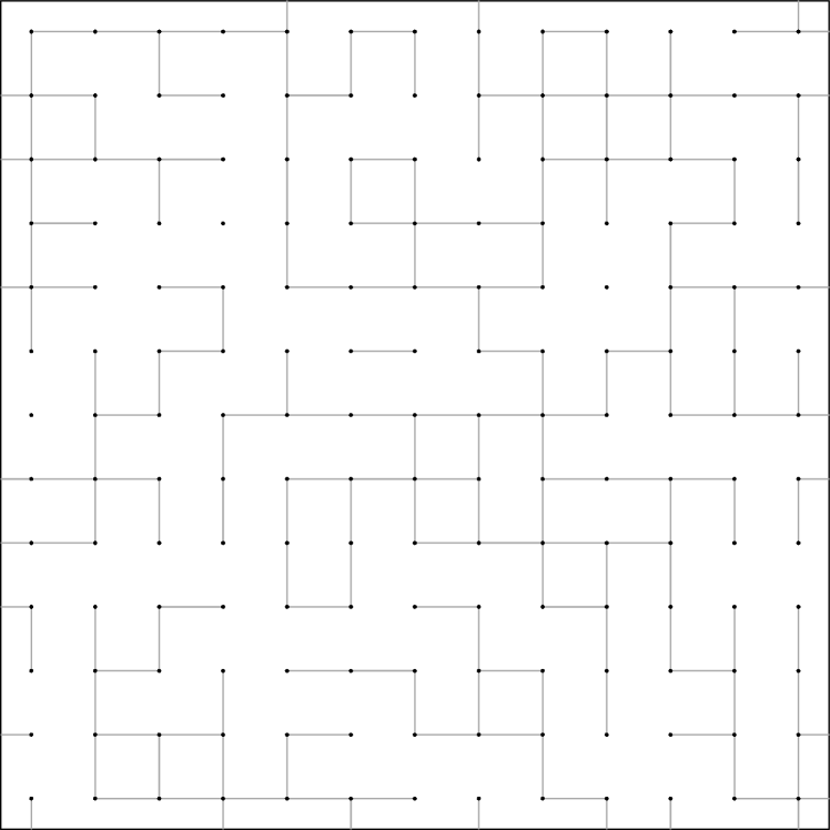
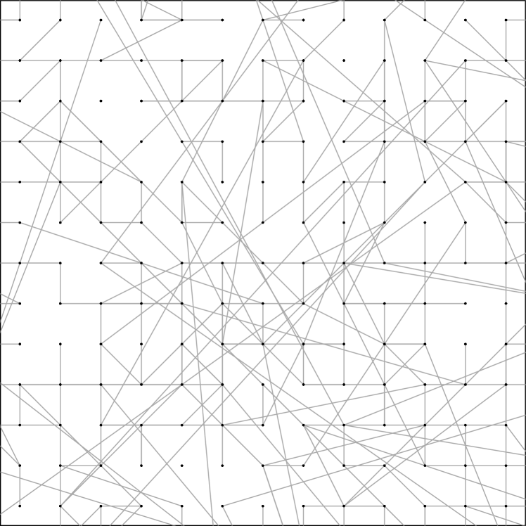
Figure 2: lhs: nearest-neighbour percolation; rhs: homogeneous long-range percolation

5 Homogeneous long-range percolation

Long-range percolation is the first extension of nearest-neighbour bond percolation. It allows for edges between any pair of particles $x,y\in{\mathbb{Z}}^{d}$. Long-range percolation was originally introduced by Schulman Schulman in one dimension. Existence and uniqueness of the infinite connected component in long-range percolation was proved by Schulman Schulman and Newman-Schulman NS for $d=1$ and by Gandolfi et al. GKN for $d\geq 2$.

Consider again the percolation model on the lattice ${\mathbb{Z}}^{d}$, but we now choose the edges differently. Choose $p\in[0,1]$, $\lambda>0$ and $\alpha>0$ fixed and define the edge probabilities for $x,y\in{\mathbb{Z}}^{d}$ by

$$p_{x,y}=\left\{\begin{array}[]{ll}p&\text{ if $\|x-y\|=1$,}\\ 1-\exp(-\lambda\|x-y\|^{-\alpha})&\text{ if $\|x-y\|>1$.}\end{array}\right.$$ (5)

Between any pair $x,y\in{\mathbb{Z}}^{d}$ we attach an edge, independently of all other edges, as follows

$$\eta_{x,y}=\eta_{y,x}=\left\{\begin{array}[]{ll}1&\text{ with probability $p_{x,y}$,}\\ 0&\text{ with probability $1-p_{x,y}$.}\end{array}\right.$$

We denote the resulting product measure on the edge configurations by ${\mathbb{P}}_{p,\lambda,\alpha}$. Figure 2 (rhs) shows part of a realised configuration. We say that the particles $x$ and $y$ are adjacent if there is an edge $\eta_{x,y}=1$ between $x$ and $y$. We say that $x$ and $y$ are connected if there exists a path of adjacent particles in ${\mathbb{Z}}^{d}$ that connects $x$ and $y$. The connected component of $x$ is given by

$${\cal C}(x)=\left\{y\in{\mathbb{Z}}^{d}:~{}\text{$x$ and $y$ are connected}\right\}.$$

We remark that the edge probabilities $p_{x,y}$ used in the literature have a more general form. Since for many results only the asymptotic behaviour of $p_{x,y}$ as $\|x-y\|\to\infty$ is relevant, we have decided to choose the explicit (simpler) form (5) because this also fits to our next models. Asymptotically we have the following power law

$$p_{x,y}~{}\sim~{}\lambda\|x-y\|^{-\alpha},\qquad\text{ as $\|x-y\|\to\infty$.}$$

Theorem 4.1 (b) immediately implies that we have percolation in ${\mathbb{Z}}^{d}$, $d\geq 2$, for $p$ sufficiently close to 1. We have the following theorem, see Theorem 1.2 in Berger Berger1 .

Theorem 5.1

For long-range percolation in ${\mathbb{Z}}^{d}$ we have, in an a.s. sense,

• for $\alpha\leq d$: there is an infinite connected component;

• for $d\geq 2$ and $\alpha>d$: for $p$ sufficiently close to 1 there is an infinite connected component;

• for $d=1$:

  • $\alpha>2$: there is no infinite connected component;

  • $1<\alpha<2$: for $p$ sufficiently close to 1 there is an infinite connected component;

  • $\alpha=2$ and $\lambda>1$: for $p$ sufficiently close to 1 there is an infinite connected component;

  • $\alpha=2$ and $\lambda\leq 1$: there is no infinite connected component.

The case $\alpha\leq d$ follows from an infinite degree distribution for a given particle, i.e. for $\alpha\leq d$ we have, a.s.,

$${\cal D}(0)=\left|\left\{x\in{\mathbb{Z}}^{d}:~{}\text{$0$ and $x$ are adjacent}\right\}\right|=\infty,$$ (6)

and for $\alpha>d$ the degree distribution is light-tailed (we give a proof in the continuum space model in Sect. 7, because the proof turns out to be straightforward in continuum space). Interestingly, we now also obtain a non-trivial phase transition in the one dimensional case $d=1$ once long-range edges are sufficiently likely, i.e. $\alpha$ is sufficiently small. At criticality $\alpha=2$ also the decay scaling constant $\lambda>0$ matters. The case $d\geq 2$ is less interesting because it is in line with nearest-neighbour bond percolation. The main interest of adding long-range edges is the study of the resulting geometric properties of connected components ${\cal C}(x)$. We will state below that there are three different regimes:

• $\alpha\leq d$ results in an infinite degree distribution, a.s., see (6);

• $d<\alpha<2d$ has finite degrees but is still in the regime of small-world behaviour;

• $\alpha>2d$ behaves as nearest-neighbour bond percolation.

We again focus on the graph distance

$$d(x,y)=\text{minimal number of edges that connect $x$ and $y$},$$ (7)

where this is defined to be infinite if $x$ and $y$ do not belong to the same connected component, i.e. $y\notin{\cal C}(x)$. For $\alpha<d$ we have infinite degrees and the infinite connected component ${\cal C}_{\infty}$ contains all particles of ${\mathbb{Z}}^{d}$, a.s. Moreover, Benjamini et al. BKPS prove in Example 6.1 that the graph distance is bounded, a.s., by

$$\left\lceil\frac{d}{d-\alpha}\right\rceil.$$

The case $\alpha\in(d,2d)$ is considered in Biskup Biskup , Theorem 1.1, and in Trapman Trapman . They have proved the following result:

Theorem 5.2

Choose $\alpha\in(d,2d)$ and assume, a.s., that there exists a unique infinite connected component ${\cal C}_{\infty}$. Then for all $\epsilon>0$ we have

$$\lim_{\|x\|\to\infty}{\mathbb{P}}_{p,\lambda,\alpha}\left[\left.\Delta-\epsilon\leq\frac{\log d(0,x)}{\log\log\|x\|}\leq\Delta+\epsilon\right|0,x\in{\cal C}_{\infty}\right]=1,$$

where $\Delta^{-1}=\log_{2}(2d/\alpha)$.

This result says that the graph distance $d(0,x)$ is roughly of order $(\log\|x\|)^{\Delta}$ with $\Delta=\Delta(\alpha,d)>1$. Unfortunately, the known bounds are not sufficiently sharp to give more precise asymptotic statements. Theorem 5.2 can be interpreted as small-world effect since it tells us that long Euclidean distances can be crossed by a few edges. For instance, $d=2$ and $\alpha=2.5$ provide $\Delta=1.47$ and we get $(\log\|x\|)^{\Delta}=26.43$ for $\|x\|=10,000$, i.e. a Euclidean distance of 10,000 is crossed in roughly 26 edges.

The case $\alpha>2d$ is considered in Berger Berger2 .

Theorem 5.3

If $\alpha>2d$ we have, a.s.,

$$\liminf_{\|x\|\to\infty}\frac{d(0,x)}{\|x\|}>0.$$

This result proves that for $\alpha>2d$ the graph distance behaves as in nearest-neighbour bond percolation, because it grows linearly in $\|x\|$. The proof of an upper bound is still open, but we expect a result similar to Theorem 4.3 in nearest-neighbour bond percolation, see Conjecture 1 of Berger Berger2 .

We conclude that this model has a small-world effect for $\alpha<2d$. It also has some kind of clustering property because particles that are close share an edge more commonly, which gives a structure that is locally more dense, see Corollary 3.4 in Biskup Biskup . But the degree distribution is light-tailed which motivates to extend the model by an additional ingredient. This is done in the next section.

6 Heterogeneous long-range percolation

Heterogeneous long-range percolation extends the previously introduced long-range percolation models on the lattice ${\mathbb{Z}}^{d}$. Deijfen et al. Remco have introduced this model under the name of scale-free percolation. The idea is to place additional weights $W_{x}$ to the particles $x\in{\mathbb{Z}}^{d}$ which determine how likely a particle may play the role of a hub in the resulting network.

Consider again the percolation model on the lattice ${\mathbb{Z}}^{d}$. Assume that $(W_{x})_{x\in{\mathbb{Z}}^{d}}$ are i.i.d. Pareto distributed with threshold parameter 1 and tail parameter $\beta>0$, i.e. for $w\geq 1$

$${\mathbb{P}}\left[W_{x}\leq w\right]=1-w^{-\beta}.$$ (8)

Choose $\alpha>0$ and $\lambda>0$ fixed. Conditionally given $(W_{x})_{x\in{\mathbb{Z}}^{d}}$, we consider the edge probabilities for $x,y\in{\mathbb{Z}}^{d}$ given by

$$p_{x,y}=1-\exp(-\lambda W_{x}W_{y}\|x-y\|^{-\alpha}).$$ (9)

Between any pair $x,y\in{\mathbb{Z}}^{d}$ we attach an edge, independently of all other edges, as follows

$$\eta_{x,y}=\eta_{y,x}=\left\{\begin{array}[]{ll}1&\text{ with probability $p_{x,y}$,}\\ 0&\text{ with probability $1-p_{x,y}$.}\end{array}\right.$$

We denote the resulting probability measure on the edge configurations by ${\mathbb{P}}_{\lambda,\alpha,\beta}$. In contrast to (5) we have additional weights $W_{x}$ and $W_{y}$ in (9). The bigger these weights the more likely is an edge between $x$ and $y$. Thus, particles $x\in{\mathbb{Z}}^{d}$ with a big weight $W_{x}$ will have many adjacent particles $y$ (i.e. particles $y\in{\mathbb{Z}}^{d}$ with $\eta_{x,y}=1$). Such particles $x$ will play the role of hubs in the network system. Figure 3 (lhs) shows part of a realised edge configuration.

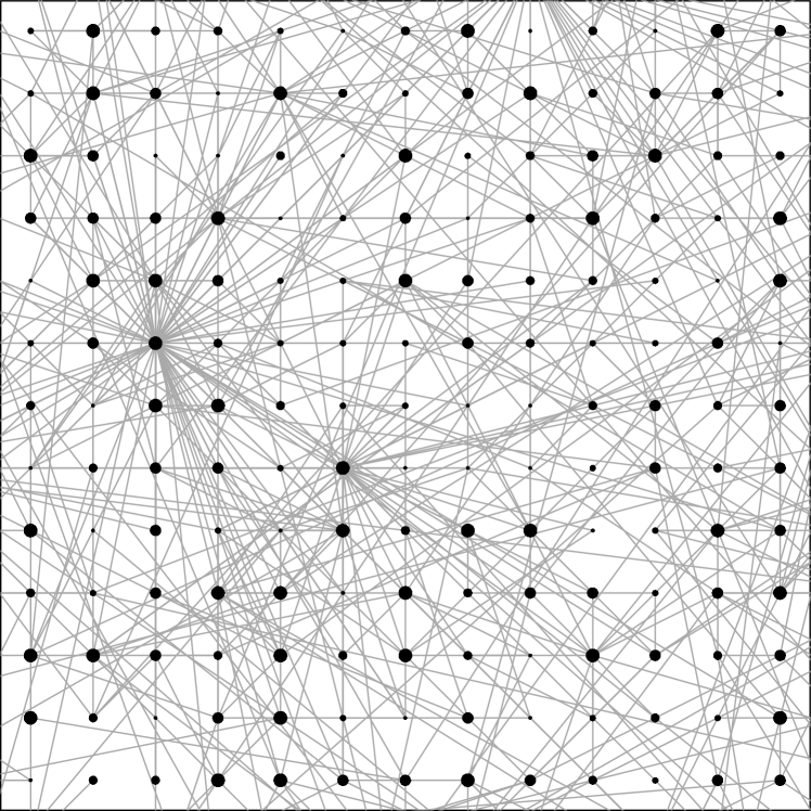
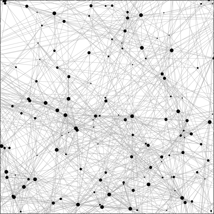
Figure 3: lhs: heterogeneous long-range percolation; rhs: continuum space long-range percolation; the size of the particles illustrates the different weights $W_{x}\geq 1$

The first interesting result is that this model provides a heavy-tailed degree distribution, see Theorems 2.1 and 2.2 in Deijfen et al. Remco . Denote again by ${\cal D}(0)$ the number of particles of ${\mathbb{Z}}^{d}$ that are adjacent to 0, then we have the following result.

Theorem 6.1

Fix $d\geq 1$. We have the following two cases for the degree distribution:

• for $\min\{\alpha,\beta\alpha\}\leq d$, a.s., ${\cal D}(0)=\infty$;

• for $\min\{\alpha,\beta\alpha\}>d$ set $\tau=\beta\alpha/d$, then

  $${\mathbb{P}}_{\lambda,\alpha,\beta}\left[{\cal D}(0)>k\right]=k^{-\tau}\ell(k),$$

  for some function $\ell(\cdot)$ that is slowly varying at infinity.

We observe that the heavy-tailedness of the weights $W_{x}$ induces heavy-tailedness in the degree distribution which is similar to choice (3) in the NSW random graph model of Sect. 3. For $\alpha>d$ there are three different regimes: (i) $\beta\alpha\leq d$ implies infinite degree, a.s.; (ii) for $d<\beta\alpha<2d$ the degree distribution has finite mean but infinite variance because $1<\tau<2$; (iii) for $\beta\alpha>2d$ the degree distribution has finite variance because $\tau>2$. We will see that the distinction of the latter two cases has also implications on the behaviour of the percolation properties and the graph distances similar to the considerations in NSW random graphs. Note that from a practical point of view the interesting regime is (ii).

We again consider the connected component of a given particle $x\in{\mathbb{Z}}^{d}$ denoted by ${\cal C}(x)$ and we define the percolation probability (for given $\alpha$ and $\beta$)

$$\theta(\lambda)={\mathbb{P}}_{\lambda,\alpha,\beta}\left[|{\cal C}(0)|=\infty\right].$$

The critical percolation value $\lambda_{c}$ is then defined by

$$\lambda_{c}=\inf\left\{\lambda>0:~{}\theta(\lambda)>0\right\}.$$

We have the following result, see Theorem 3.1 in Deijfen et al. Remco .

Theorem 6.2

Fix $d\geq 1$. Assume $\min\{\alpha,\beta\alpha\}>d$.

• If $d\geq 2$, then $\lambda_{c}<\infty$.

• If $d=1$ and $\alpha\in(1,2]$, then $\lambda_{c}<\infty$.

• If $d=1$ and $\min\{\alpha,\beta\alpha\}>2$, then $\lambda_{c}=\infty$.

This result is in line with Theorem 5.1. Since $W_{x}\geq 1$, a.s., an edge configuration from edge probabilities $p_{x,y}$ defined in (9) stochastically dominates an edge configuration with edge probabilities $1-\exp(-\lambda\|x-y\|^{-\alpha})$. The latter is similar to the homogeneous long-range percolation model on ${\mathbb{Z}}^{d}$ and the results of the above theorem directly follow from Theorem 5.1. For part (c) of the theorem we also refer to Theorem 3.1 of Deijfen et al. Remco . The next theorem follows from Theorems 4.2 and 4.4 of Deijfen et al. Remco .

Theorem 6.3

Fix $d\geq 1$. Assume $\min\{\alpha,\beta\alpha\}>d$.

• If $\beta\alpha<2d$, then $\lambda_{c}=0$.

• If $\beta\alpha>2d$, then $\lambda_{c}>0$.

Theorems 6.2 and 6.3 give the phase transition pictures for $d\geq 1$, see Fig. 4 for an illustration. They differ for $d=1$ and $d\geq 2$ in that the former has a region where $\lambda_{c}=\infty$ and the latter does not, see also the distinction in Theorem 5.1. The most interesting case from a practical point of view is the infinite variance case, $1<\tau<2$ and $d<\beta\alpha<2d$, respectively, which provides percolation for any $\lambda>0$. It follows from Gandolfi et al. GKN that there is only one infinite connected component $\mathcal{C}_{\infty}$ whenever $\lambda>\lambda_{c}$, a.s. A difficult question to answer is what happens at criticality for $\lambda_{c}>0$. There is the following partial result, see Theorem 3 in Deprez et al. HW : for $\alpha\in(d,2d)$ and $\beta\alpha>2d$, there does not exist an infinite connected component at criticality $\lambda_{c}>0$. The case $\min\{\alpha,\beta\alpha\}>2d$ is still open.

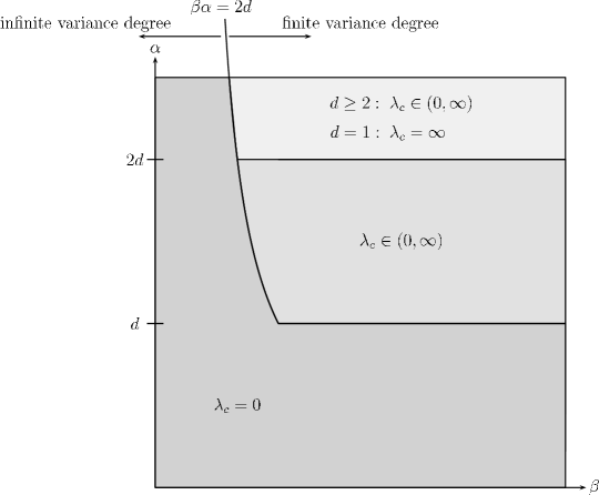
Figure 4: phase transition picture for $d\geq 1$

Next we consider the graph distance $d(x,y)$, see also (7). We have the following result, see Deijfen et al. Remco and Theorem 8 in Deprez et al. HW .

Theorem 6.4

Assume $\min\{\alpha,\beta\alpha\}>d$.

• (infinite variance of degree distribution $1<\tau<2$). Assume $d<\beta\alpha<2d$. For any $\lambda>\lambda_{c}=0$ there exists $\eta_{1}>0$ such that for all $\epsilon>0$

  $$\lim_{\|x\|\to\infty}{\mathbb{P}}_{\lambda,\alpha,\beta}\left[\left.\eta_{1}\leq\frac{d(0,x)}{\log\log\|x\|}\leq\frac{2}{|\log(\beta\alpha/d-1)|}+\epsilon\right|0,x\in{\cal C}_{\infty}\right]=1.$$

• (finite variance of degree distribution $\tau>2$ case 1). Assume that $\beta\alpha>2d$ and $\alpha\in(d,2d)$. For any $\lambda>\lambda_{c}$ there exists $\eta_{2}\geq 1$ such that for all $\epsilon>0$

  $$\lim_{\|x\|\to\infty}{\mathbb{P}}_{\lambda,\alpha,\beta}\left[\left.\eta_{2}-\epsilon\leq\frac{\log d(0,x)}{\log\log\|x\|}\leq\Delta+\epsilon\right|0,x\in{\cal C}_{\infty}\right]=1,$$

  where $\Delta$ was defined in Theorem 5.2.

• (finite variance of degree distribution $\tau>2$ case 2). Assume $\min\{\alpha,\beta\alpha\}>2d$. There exists $\eta_{3}>0$ such that

  $$\lim_{\|x\|\to\infty}{\mathbb{P}}_{\lambda,\alpha,\beta}\left[\eta_{3}<\frac{d(0,x)}{\|x\|}\right]=1.$$

Compare Theorem 6.4 (heterogeneous case) to Theorems 5.2 and 5.3 (homogeneous case). We observe that in the finite variance cases (b1)–(b2), i.e. for $\tau=\beta\alpha/d>2$, we obtain the same behaviour for heterogeneous and homogeneous long-range percolation models. The infinite variance case (a) of the degree distribution, i.e. $1<\tau<2$ and $d<\beta\alpha<2d$, respectively, is new. This infinite variance case provides a much slower decay of the graph distance, that is $d(0,x)$ is of order $\log\log\|x\|$ as $\|x\|\to\infty$. This is a pronounced version of the small-world effect, and this behaviour is similar to the NSW random graph model. Recall that empirical studies often suggest a tail parameter $\tau$ between 1 and 2 which corresponds to the infinite variance regime of the degree distribution. In Fig. 5 we illustrate Theorem 6.4 and we complete the picture about the chemical distances with the corresponding conjectures.

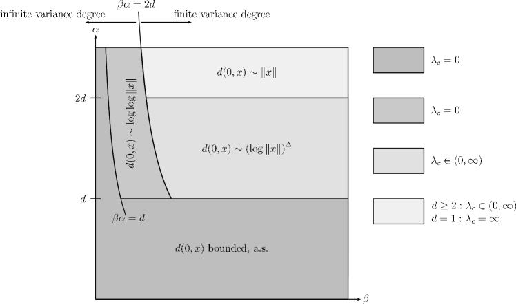
Figure 5: chemical distances according to Theorem 6.4 and corresponding conjectures

We conclude that this model fulfils all three stylised facts of small-world effect, the clustering property (which is induced by the Euclidean distance in the probability weights (9)) and the heavy-tailedness of the degree distribution.

7 Continuum space long-range percolation model

The model of last section is restricted to the lattice ${\mathbb{Z}}^{d}$. A straightforward modification is to replace the lattice ${\mathbb{Z}}^{d}$ by a homogeneous Poisson point process $X$ in ${\mathbb{R}}^{d}$. In comparison to the lattice model, some of the proofs simplify because we can apply classical integration in ${\mathbb{R}}^{d}$, other proofs become more complicated because one needs to make sure that the realisation of the Poisson point process is sufficiently regular in space. As in Deprez-Wüthrich DW we consider a homogeneous marked Poisson point process in ${\mathbb{R}}^{d}$, where

• $X$ denotes the spatially homogeneous Poisson point process in ${\mathbb{R}}^{d}$ with constant intensity $\nu>0$. The individual particles of $X$ are denoted by $x\in X\subset{\mathbb{R}}^{d}$;

• $W_{x}$, $x\in X$, are i.i.d. marks having a Pareto distribution with threshold parameter 1 and tail parameter $\beta>0$, see (8).

Choose $\alpha>0$ and $\lambda>0$ fixed. Conditionally given $X$ and $(W_{x})_{x\in X}$, we consider the edge probabilities for $x,y\in X$ given by

$$p_{x,y}=1-\exp(-\lambda W_{x}W_{y}\|x-y\|^{-\alpha}).$$ (10)

Between any pair $x,y\in X$ we attach an edge, independently of all other edges, as follows

$$\eta_{x,y}=\eta_{y,x}=\left\{\begin{array}[]{ll}1&\text{ with probability $p_{x,y}$,}\\ 0&\text{ with probability $1-p_{x,y}$.}\end{array}\right.$$

We denote the resulting probability measure on the edge configuration by ${\mathbb{P}}_{\nu,\lambda,\alpha,\beta}$. Figure 3 (rhs) shows part of a realised configuration. We have the following result for the degree distribution, see Proposition 3.2 and Theorem 3.3 in Deprez-Wüthrich DW .

Theorem 7.1

Fix $d\geq 1$. We have the following two cases for the degree distribution:

• for $\min\{\alpha,\beta\alpha\}\leq d$, a.s., ${\mathbb{P}}_{0}[{\cal D}(0)=\infty|W_{0}]=1$;

• for $\min\{\alpha,\beta\alpha\}>d$ set $\tau=\beta\alpha/d$, then

  $${\mathbb{P}}_{0}\left[{\cal D}(0)>k\right]=k^{-\tau}\ell(k),$$

  for some function $\ell(\cdot)$ that is slowly varying at infinity.

Remarks.

• Note that the previous statement needs some care because we need to make sure that there is a particle at the origin. This is not straightforward in the Poisson case and ${\mathbb{P}}_{0}$ can be understood as the conditional distribution, conditioned on having a particle at the origin. The formally precise construction is known as the Palm distribution, which considers distributions shifted by the particles in the Poisson cloud $X$.

• In analogy to the homogeneous long-range percolation model in ${\mathbb{Z}}^{d}$ we could also consider continuum space homogeneous long-range percolation in ${\mathbb{R}}^{d}$. This is achieved by setting $W_{x}=W_{y}=1$, a.s., in (10). In this case the proof of the statement equivalent to (6) becomes rather easy. We briefly give the details in the next lemma, see also proof of Lemma 3.1 in Deprez-Wüthrich DW .

Lemma 1

Choose $W_{x}=W_{y}=1$, a.s., in (10). For $\alpha\leq d$ we have, a.s., ${\cal D}(0)=\infty$; for $\alpha>d$ the degree ${\cal D}(0)$ has a Poisson distribution.

Proof of Lemma 1 and (6) in continuum space.  Let $X$ be a Poisson cloud with $0\in X$ and denote by $X(A)$ the number of particles in $X\cap A$ for $A\subset{\mathbb{R}}^{d}$. Every particle $x\in X\setminus\{0\}$ is now independently from the others removed from the Poisson cloud with probability $1-p_{0,x}$. The resulting process $\widetilde{X}$ is a thinned Poisson cloud having intensity function $x\mapsto\nu p_{0,x}=\nu(1-\exp(-\lambda\|x\|^{-\alpha}))\sim\nu\lambda\|x\|^{-\alpha}$ as $\|x\|\to\infty$. Since $\mathcal{D}(0)=\tilde{X}({\mathbb{R}}^{d}\setminus\{0\})$ it follows that $\mathcal{D}(0)$ is infinite, a.s., if $\alpha\leq d$ and that $\mathcal{D}(0)$ has a Poisson distribution otherwise. To see this let $\mu$ denote the Lebesgue measure in ${\mathbb{R}}^{d}$ and choose a finite Borel set $A\subset{\mathbb{R}}^{d}$ containing the origin. Since $A$ contains the origin, we have $X(A)\geq\widetilde{X}(A)\geq 1$. This motivates for $k\in\mathbb{N}_{0}$ to study

$${\mathbb{P}}_{0}\left[\widetilde{X}(A)=k+1\right] = \sum_{i\geq k}{\mathbb{P}}_{0}\left[\left.\widetilde{X}(A)=k+1\right|X(A)=i+1\right]{\mathbb{P}}_{0}\left[{X}(A)=i+1\right].$$

Since $A$ contains the origin, the case $i=0$ is trivial, i.e. ${\mathbb{P}}_{0}[\widetilde{X}(A)=1|X(A)=1]=1$. There remains $i\geq 1$. Conditionally on $\{{X}(A)=i+1\}$, the $i$ particles (excluding the origin) are independent and uniformly distributed in $A$. The conditional moment generating function for $r\in{\mathbb{R}}$ is then given by

$${\mathbb{E}}_{0}\left[\left.\exp\left\{r\left(\widetilde{X}(A)-1\right)\right\}\right|X(A)=i+1\right]$$

$$=~{}\frac{1}{\mu(A)^{i}}\int_{A\times\cdots\times A}{\mathbb{E}}_{0}\left[\exp\left\{r\sum_{l=1}^{i}\eta_{0,x_{l}}\right\}\right]dx_{1}\cdots dx_{i}$$

$$=~{}\frac{1}{\mu(A)^{i}}\int_{A\times\cdots\times A}\prod_{l=1}^{i}{\mathbb{E}}_{0}\left[\exp\left\{r\eta_{0,x_{l}}\right\}\right]dx_{1}\cdots dx_{i}$$

$$=~{}\left(\frac{1}{\mu(A)}\int_{A}{\mathbb{E}}_{0}\left[\exp\left\{r\eta_{0,x}\right\}\right]dx\right)^{i}.$$

We calculate the integral for $W_{0}=W_{x}=1$, a.s., in (10)

$$\frac{1}{\mu(A)}\int_{A}{\mathbb{E}}_{0}\left[\exp\left\{r\eta_{0,x}\right\}\right]dx = \frac{1}{\mu(A)}\int_{A}e^{r}p_{0,x}+(1-p_{0,x})~{}dx$$

$$= e^{r}p(A)+\left(1-p(A)\right),$$

with $p(A)=\mu(A)^{-1}\int_{A}p_{0,x}dx\in(0,1)$. Thus, conditionally on $\{X(A)=i+1\}$, $\widetilde{X}(A)-1$ has a binomial distribution with parameters $i$ and $p(A)$. This implies that

$${\mathbb{P}}_{0}\left[\widetilde{X}(A)=k+1\right] = \sum_{i\geq k}\binom{i}{k}~{}p(A)^{k}\left(1-p(A)\right)^{i-k}~{}{\mathbb{P}}_{0}\left[{X}(A)=i+1\right]$$

$$= \sum_{i\geq k}\frac{p(A)^{k}}{k!}\frac{\left(1-p(A)\right)^{i-k}}{(i-k)!}~{}\exp\{-\nu\mu(A)\}(\nu\mu(A))^{i}$$

$$= \frac{(\nu\mu(A)p(A))^{k}}{k!}\sum_{i\geq k}\frac{\left(\nu\mu(A)(1-p(A))\right)^{i-k}}{(i-k)!}\exp\{-\nu\mu(A)\}$$

$$= \exp\left\{-\nu\mu(A)p(A)\right\}\frac{(\nu\mu(A)p(A))^{k}}{k!}$$

$$= \exp\left\{-\nu\int_{A}p_{0,x}dx\right\}\frac{\left(\nu\int_{A}p_{0,x}dx\right)^{k}}{k!}.$$

This implies that $\widetilde{X}$ is a non-homogeneous Poisson point process with intensity function

$$x\mapsto\nu p_{0,x}=\nu\left(1-\exp(-\lambda\|x\|^{-\alpha})\right)\sim\nu\lambda\|x\|^{-\alpha},\qquad\text{ as $\|x\|\to\infty$.}$$

But this immediately implies that the degree distribution ${\cal D}(0)=\widetilde{X}({\mathbb{R}}^{d}\setminus\{0\})$ is infinite, a.s., if $\alpha\leq d$, and that it has a Poisson distribution otherwise. This finishes the proof. ∎

We now switch back to the heterogeneous long-range percolation model (10). We consider the connected component $\mathcal{C}(0)$ of a particle in the origin under the Palm distribution ${\mathbb{P}}_{0}$. We define the percolation probability

$$\theta(\lambda)={\mathbb{P}}_{0}\left[|{\cal C}(0)|=\infty\right].$$

The critical percolation value $\lambda_{c}$ is then defined by

$$\lambda_{c}=\inf\left\{\lambda>0:~{}\theta(\lambda)>0\right\}.$$

We have the following results, see Theorem 3.4 in Deprez-Wüthrich DW .

Theorem 7.2

Fix $d\geq 1$. Assume $\min\{\alpha,\beta\alpha\}>d$.

• If $d\geq 2$, then $\lambda_{c}<\infty$.

• If $d=1$ and $\alpha\in(1,2]$, then $\lambda_{c}<\infty$.

• If $d=1$ and $\min\{\alpha,\beta\alpha\}>2$, then $\lambda_{c}=\infty$.

Theorem 7.3

Fix $d\geq 1$. Assume $\min\{\alpha,\beta\alpha\}>d$.

• If $\beta\alpha<2d$, then $\lambda_{c}=0$.

• If $\beta\alpha>2d$, then $\lambda_{c}>0$.

These are the continuum space analogues to Theorems 6.2 and 6.3, for an illustration see also Fig. 4. The work on the graph distances in the continuum space long-range percolation model is still work in progress, but we expect similar results to the ones in Theorem 6.4, see also Fig. 5. However, proofs in the continuum space model are more sophisticated due to the randomness of the positions of the particles.

The advantage of the latter continuum space model (with homogeneous marked Poisson point process) is that it can be extended to non-homogeneous Poisson point processes. For instance, if certain areas are more densely populated than others we can achieve such a non-homogeneous space model by modifying the constant intensity $\nu$ to a space-dependent density function $\nu(\cdot):{\mathbb{R}}^{d}\to{\mathbb{R}}_{+}$.

8 Renormalisation techniques

In this section we present a crucial technique that is used in many of the proofs of the previous statements. These proofs are often based on renormalisation techniques. That is, one collects particles in boxes. These boxes are defined to be either good (having a certain property) or bad (not possessing this property). These boxes are then again merged to bigger good or bad boxes. These scalings and renormalisations are done over several generations of box sizes, see Fig. 6 for an illustration. The purpose of these rescalings is that one arrives at a certain generation of box sizes that possesses certain characteristics to which classical site-bond percolation results apply. We exemplify this with a particular example.

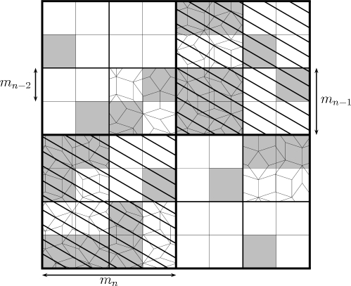
Figure 6: Example of the renormalisation technique. Define inductively the box lengths $m_{n}=2m_{n-1}$, $n\in\mathbb{N}$, for some initial $m_{0}\in\mathbb{N}$. Call translates of $[0,m_{0}-1]^{d}$ to be $0$-stage boxes and assume that goodness of such boxes is defined. For $n\in\mathbb{N}$ we call the translates of $[0,m_{n}-1]^{d}$ $n$-stage boxes and we inductively say that an $n$-stage box is good if it contains at least two good $(n-1)$-stage boxes. Assume that in the illustration good $(n-2)$-stage boxes, $n\geq 2$, are coloured in grey. The good $(n-1)$-stage boxes are then the Penrose-patterned boxes of side-length $m_{n-1}$ and the good $n$-stage boxes are striped. The illustrated $(n+1)$-stage box is good, because it contains two good $n$-stage boxes

8.1 Site-bond percolation

Though we will not directly use site-bond percolation, we start with the description of this model because it is often useful. Site-bond percolation in ${\mathbb{Z}}^{d}$ is a modification of homogeneous long-range percolation introduced in Sect. 5. Choose a fixed dimension $d\geq 1$ and consider the square lattice ${\mathbb{Z}}^{d}$. Assume that every site $x\in{\mathbb{Z}}^{d}$ is occupied independently with probability $r^{\ast}\in[0,1]$ and every bond between $x$ and $y$ in ${\mathbb{Z}}^{d}$ is occupied independently with probability

$$p^{\ast}_{x,y}=1-\exp(-\lambda^{\ast}\|x-y\|^{-\alpha}),$$ (11)

for given parameters $\lambda^{\ast}>0$ and $\alpha>0$. The connected component ${\cal C}^{\ast}(x)$ of a given site $x\in{\mathbb{Z}}^{d}$ is then defined to be the set of all occupied sites $y\in{\mathbb{Z}}^{d}$ such that $x$ and $y$ are connected by a path only running through occupied sites and occupied bonds (if $x$ is not occupied then ${\cal C}^{\ast}(x)$ is the empty set). We can interpret this as follows: we place particles at sites $x\in{\mathbb{Z}}^{d}$ at random with probability $r^{\ast}$. This defines a (random) subset of ${\mathbb{Z}}^{d}$ and then we consider long-range percolation on this random subset, i.e. this corresponds to a thinning of homogeneous long-range percolation in ${\mathbb{Z}}^{d}$. We can then study the percolation properties of this site-bond percolation model, some results are presented in Lemma 3.6 of Biskup Biskup and in the proof of Theorem 2.5 of Berger Berger1 . The aim in many proofs in percolation theory is to define different generations of box sizes using renormalisations, see Fig. 6. We perform these renormalisations until we arrive at a generation of box sizes for which good boxes occur sufficiently often. If this is the case and if all the necessary dependence assumptions are fulfilled we can apply classical site-bond percolation results.

In order to simplify our outline we use a modified version of the homogeneous long-range percolation model (5) of Sect. 5. We set $p=1-\exp(-\lambda)$ and obtain the following model.

Model 8.1 (modified homogeneous long-range percolation)

Fix $d\geq 2$. Choose $\alpha>0$ and $\lambda>0$ fixed and define the edge probabilities for $x,y\in{\mathbb{Z}}^{d}$ by

$$p_{x,y}=1-\exp(-\lambda\|x-y\|^{-\alpha}).$$

Then edges between all pairs of particles $x,y\in{\mathbb{Z}}^{d}$ are attached independently with edge probability $p_{x,y}$ and the probability measure of the resulting edge configurations $\eta=(\eta_{x,y})_{x,y\in{\mathbb{Z}}^{d}}$ is denoted by ${\mathbb{P}}_{\lambda,\alpha}$.

Note that this model is a special case of site-bond percolation with $r^{\ast}=1$ and $\lambda^{\ast}=\lambda$ in (11).

8.2 Largest semi-clusters

In order to demonstrate the renormalisation technique we repeat the proof of Lemma 2.3 of Berger Berger1 in the modified homogeneous long-range percolation Model 8.1, see Theorem 8.2 below. This proof is rather sophisticated because it needs a careful treatment of dependence and we revisit the second version of the proof of Lemma 2.3 provided in Berger Berger11 .

Fix $\alpha\in(d,2d)$ and choose $\lambda>0$ so large that there exists a unique infinite connected component, a.s., having density $\kappa>0$ (which exists due to Theorem 5.1). Choose $M\geq 1$ and $K\geq 0$ integer valued. For $v\in{\mathbb{Z}}^{d}$ we define box $B_{v}$ and its $K$-enlargement $B^{(K)}_{v}$ by

$$B_{v}=Mv+[0,M-1]^{d}\qquad\text{ and }\qquad B^{(K)}_{v}=Mv+[-K,M+K-1]^{d}.$$

For every box $B_{v}$ we define a $\ell$-semi-cluster to be a set of at least $\ell$ sites in $B_{v}$ which are connected within $B_{v}^{(K)}$. For any $\varepsilon>0$ there exists $M^{\prime}\geq 1$ such that for all $M\geq M^{\prime}$ and some $K\geq 0$ we have

$${\mathbb{P}}_{\lambda,\alpha}[\text{at least $M^{d}\kappa/2$ sites of $B_{v}$ belong to the infinite connected }~{}$$ (12)

$$\text{component and these sites are connected within $B^{(K)}_{v}$}] \geq 1-\varepsilon/2.$$

Existence of $M^{\prime}\geq 1$ follows from the ergodic theorem and existence of $K$ from the fact that the infinite connected component is unique, a.s., and therefore all sites in $B_{v}$ belonging to the infinite connected component need to be connected within a certain $K$-enlargement of $B_{v}$. Formula (12) says that we have a $(M^{d}\kappa/2)$-semi-cluster in $B_{v}$ with at least probability $1-\varepsilon/2$. We first show uniqueness of large semi-clusters.

Lemma 2

Choose $\xi\in(\alpha/d,2)$ and $\gamma\in(0,1)$ with $18\gamma>16+\xi$. There exist $\varphi=\varphi(\xi,\gamma)>0$ and $M^{\prime}=M^{\prime}(\xi,\gamma)\geq 1$ such that for all $M\geq M^{\prime}$ and all $K\geq 0$ we have

$${\mathbb{P}}_{\lambda,\alpha}\left[\text{there is at most one $M^{d\gamma}$-semi-cluster in $B_{v}$}\right]>1-M^{-d\varphi},$$

where by “at most one” we mean that there is no second $M^{d\gamma}$-semi-cluster in $B_{v}$ which is not connected to the first one within $B_{v}^{(K)}$.

Proof of Lemma 2. The proof uses the notion of inhomogeneous random graphs as defined in Aldous Aldous . An inhomogeneous random graph $H(N,\xi)$ with size $N$ and parameter $\xi$ is a set of particles $\{1,\ldots,k\}$ and corresponding masses $s_{1},\ldots,s_{k}$ such that $N=\sum_{i=1}^{k}s_{i}$; and any $i\neq j$ are connected independently with probability $1-\exp\left(-s_{i}s_{j}N^{-\xi}\right)$. From Lemma 2.5 of Berger Berger11 we know that for any $1<\xi<2$ and $0<\gamma<1$ with $18\gamma>16+\xi$, there exist $\varphi=\varphi(\xi,\gamma)>0$ and $N^{\prime}=N^{\prime}(\xi,\gamma)\geq 1$ such that for all $N\geq N^{\prime}$ and every inhomogeneous random graph with size $N$ and parameter $\xi$ we have

$${\mathbb{P}}\left[\text{$H(N,\xi)$ contains more than one connected component $C$ with $\sum_{i\in C}s_{i}\geq N^{\gamma}$}\right]$$

$$<~{}N^{-\varphi}.$$ (13)

We now show uniqueness of $M^{d\gamma}$-semi-clusters in $B_{v}$. Choose $\xi\in(\alpha/d,2)$ and $\gamma\in(0,1)$ such that $18\gamma>16+\xi$. For any $x,y\in B_{v}$ we have $\|x-y\|\leq\sqrt{d}M$. Choose $M$ so large that $\lambda(\sqrt{d}M)^{-\alpha}>M^{-d\xi}$ and choose $K\geq 0$ arbitrarily. Particles $x,y\in B_{v}$ are then attached with probability $p_{x,y}$ uniformly bounded by

$$p_{x,y} = 1-\exp(-\lambda\|x-y\|^{-\alpha})$$

$$\geq 1-\exp\left(-\lambda\left(\sqrt{d}M\right)^{-\alpha}\right)>1-\exp\left(-M^{-d\xi}\right)=\nu>0,$$

where the last equality defines $\nu$. This allows to decouple the sampling of edges $\eta=(\eta_{x,y})_{x,y\in{\mathbb{Z}}^{d}}$ in $B_{v}$. For every $x,y\in B_{v}$, define $p^{\prime}_{x,y}\in(0,1)$ by

$$p_{x,y}=p^{\prime}_{x,y}+\nu-\nu p^{\prime}_{x,y}.$$

We now sample $\eta=(\eta_{x,y})_{x,y\in{\mathbb{Z}}^{d}}$ in two steps. We first sample $\eta^{\prime}$ according to Model 8.1 but with edge probabilities $p^{\prime}_{x,y}$ if $x,y\in B_{v}$ and with edge probabilities $p_{x,y}$ otherwise. Secondly, we sample $\eta^{\prime\prime}$ as an independent configuration on $B_{v}$ where there is an edge between $x$ and $y$ with edge probability $\nu$ for $x,y\in B_{v}$. By definition of $p^{\prime}_{x,y}$ we get that $\eta^{\prime}\vee\eta^{\prime\prime}\stackrel{{\scriptstyle\rm(d)}}{{=}}\eta$. Let $S_{1},S_{2}\subset B_{v}$ be two disjoint maximal sets of sites in $B_{v}$ that are $\eta^{\prime}$-connected within $B_{v}^{(K)}$, i.e. $S_{1}$ and $S_{2}$ are two disjoint maximal semi-clusters in $B_{v}$ for given edge configuration $\eta^{\prime}$. Note that by maximality

$${\mathbb{P}}\left[\left.\text{there is an $\eta$-edge between $S_{1}$ and $S_{2}$}\right|\eta^{\prime}\right]$$

$$={\mathbb{P}}\left[\left.\text{there is an $\eta^{\prime\prime}$-edge between $S_{1}$ and $S_{2}$}\right|\eta^{\prime}\right]$$

$$=1-(1-\nu)^{|S_{1}||S_{2}|}~{}=~{}1-\exp\left(-|S_{1}||S_{2}|M^{-d\xi}\right).$$

If we denote by $S_{1},\ldots,S_{k}$ all disjoint maximal semi-clusters in $B_{v}$ for given edge configuration $\eta^{\prime}$ then we see that these maximal semi-clusters form an inhomogeneous random graph of size $\sum_{i=1}^{k}|S_{i}|=M^{d}$ and parameter $\xi$. Therefore, there exist $\varphi>0$ and $M^{\prime}\geq 1$ such that for all $M\geq M^{\prime}$ and all $K\geq 0$ we have from (8.2)

$${\mathbb{P}}\Bigg{[}\text{$H(M^{d},\xi)$ contains more than one connected component $C$}~{}$$

$$\hskip 170.71652pt\text{with $\sum_{i\in C}|S_{i}|\geq M^{d\gamma}$}\Bigg{|}\eta^{\prime}\Bigg{]}<M^{-d\varphi}.$$

Note that this bound is uniform in $\eta^{\prime}$ and $K\geq 0$. Therefore, the probability of having at least two $M^{d\gamma}$-semi-clusters in $B_{v}$ which are not connected within $B_{v}^{(K)}$ is bounded by $M^{-d\varphi}$. ∎

We can now combine (12) and Lemma 2. Choose $\varepsilon>0$. For all $M$ sufficiently large and $K\geq 0$ such that (12) holds we have

$${\mathbb{P}}_{\lambda,\alpha}\left[\text{there is exactly one $(M^{d}\kappa/2)$-semi-cluster in $B_{v}$}\right]\geq 1-\varepsilon,$$ (14)

where by “exactly one” we mean that there is no other $(M^{d}\kappa/2)$-semi-cluster in $B_{v}$ which is not connected to the first one within $B_{v}^{(K)}$. This follows because of $\gamma<1$, which implies that $M^{d\gamma}\leq M^{d}\kappa/2$ for all $M$ sufficiently large, and because $M^{-d\varphi}<\varepsilon/2$ for all $M$ sufficiently large.

8.3 Renormalisation

Choose $\varepsilon>0$ fixed, and $M>1$ and $K\geq 0$ such that (14) holds. For $v\in{\mathbb{Z}}^{d}$ we say that box $B_{v}$ is good if there is exactly one $(M^{d}\kappa/2)$-semi-cluster in $B_{v}$ (where exactly one is meant in the sense of above). Therefore, on good boxes there are at least $M^{d}\kappa/2$ sites in $B_{v}$ that are connected within $B^{(K)}_{v}$ and we have

$${\mathbb{P}}_{\lambda,\alpha}[\text{$B_{v}$ is good}]\geq 1-\varepsilon.$$ (15)

Note that the goodness properties of $B_{v_{1}}$ and $B_{v_{2}}$ for $v_{1}\neq v_{2}\in{\mathbb{Z}}^{d}$ are not necessarily independent because their $K$-enlargements $B^{(K)}_{v_{1}}$ and $B^{(K)}_{v_{2}}$ may overlap.

Now, we define renormalisation over different generations $n\in\mathbb{N}_{0}$; terminology $n$-stage is referred to the $n$-th generation. Choose an integer valued sequence $a_{n}>1$, $n\in\mathbb{N}_{0}$, with $a_{0}=M$ and define the box lengths $(M_{n})_{n\in\mathbb{N}_{0}}$ as follows: set $M_{0}=a_{0}=M$ and for $n\in\mathbb{N}$

$$M_{n}=a_{n}M_{n-1}=M_{0}\prod_{i=1}^{n}a_{i}=\prod_{i=0}^{n}a_{i}.$$

Define the $n$-stage boxes, $n\in\mathbb{N}_{0}$, by

$$B_{n,v}=M_{n}v+[0,M_{n}-1]^{d}\qquad\text{ with $v\in{\mathbb{Z}}^{d}$.}$$

Note that $n$-stage boxes $B_{n,v}$ have volume $M^{d}_{n}=a_{n}^{d}M^{d}_{n-1}=\prod_{i=0}^{n}a^{d}_{i}$ and every $n$-stage box $B_{n,v}$ contains $a_{n}^{d}$ of $(n-1)$-stage boxes $B_{n-1,x}\subset B_{n,v}$, and $(M_{n}/a_{0})^{d}=\prod_{i=1}^{n}a^{d}_{i}$ of $0$-stage boxes $B_{x}=B_{0,x}\subset B_{n,v}$, see also Fig. 6.

Renormalisation. We define goodness of $n$-stage boxes $B_{n,v}$ recursively for a given sequence $\kappa_{n}\in(0,1)$, $n\in\mathbb{N}_{0}$, of densities where we initialise $\kappa_{0}=\kappa/2$.

(i) Initialisation $n=0$. We say that $0$-stage box $B_{0,v}$, $v\in{\mathbb{Z}}^{d}$, is good if it contains exactly one $(\kappa_{0}a_{0}^{d})$-semi-cluster. Due to our choices of $M>1$ and $K\geq 0$ we see that the goodness of $0$-stage box $B_{0,v}$ occurs with at least probability $1-\varepsilon$, see (15).

(ii) Iteration $n-1\to n$. Choose $n\in\mathbb{N}$ and assume that goodness of $(n-1)$-stage boxes $B_{n-1,v}$, $v\in{\mathbb{Z}}^{d}$, has been defined. For $v\in{\mathbb{Z}}^{d}$ we say that $n$-stage box $B_{n,v}$ is good if the event $A_{n,v}=A^{(a)}_{n,v}\cap A^{(b)}_{n,v}$ occurs, where

• $A^{(a)}_{n,v}=\{\text{at least $\kappa_{n}a_{n}^{d}$ of the $(n-1)$-stage boxes $B_{n-1,x}\subset B_{n,v}$ are good}\}$; and

• $A^{(b)}_{n,v}=\{\text{all $(\prod_{i=0}^{n-1}\kappa_{i}a_{i}^{d})$-semi-clusters of all good $(n-1)$-stage boxes }$
  $\text{\hskip 170.71652pt in $B_{n,v}$ are connected within $B^{(K)}_{n,v}$}\}$.

∎

Observe that on event $A_{n,v}$ the $n$-stage box $B_{n,v}$ contains at least $\prod_{i=0}^{n}\kappa_{i}a_{i}^{d}$ sites that are connected within the $K$-enlargement $B^{(K)}_{n,v}$ of $B_{n,v}$. We set density $u_{n}=\prod_{i=0}^{n}\kappa_{i}$ which gives

$$\prod_{i=0}^{n}\kappa_{i}a_{i}^{d}=M_{n}^{d}\prod_{i=0}^{n}\kappa_{i}=M_{n}^{d}u_{n}.$$

Therefore, good $n$-stage boxes contain $(M_{n}^{d}u_{n})$-semi-clusters. Our next aim is to calculate the probability $p_{n}$ of having a good $n$-stage box. The case $n=0$ follows from (15), i.e. for any $\varepsilon>0$ and any $M$ sufficiently large there exists $K\geq 0$ such that

$$p_{0}~{}=~{}{\mathbb{P}}_{\lambda,\alpha}[\text{$B_{0,v}$ is good}]~{}=~{}{\mathbb{P}}_{\lambda,\alpha}[\text{$B_{v}$ is good}]~{}\geq~{}1-\varepsilon.$$

Theorem 8.2

Assume $\alpha\in(d,2d)$. Choose $\lambda>0$ so large that we have a unique infinite connected component, a.s., having density $\kappa>0$. For every $\varepsilon^{\prime}\in(0,1)$ there exists $N_{0}\geq 1$ such that for all $N\geq N_{0}$

$${\mathbb{P}}_{\lambda,\alpha}\left[|C_{N}|\geq N^{\alpha/2}\right]\geq 1-\varepsilon^{\prime},$$

where $C_{N}$ is the largest connected component in $[0,N-1]^{d}$.

Note that for density $\kappa>0$ of the infinite connected component we expect roughly $\kappa N^{d}$ sites in box $[0,N-1]^{d}$ belonging to the infinite connected component. The above lemma however says that at least $N^{\alpha/2}$ sites in $[0,N-1]^{d}$ are connected within that box. That is, here we do not need any $K$-enlargements as in (12) and, therefore, this event is independent for different disjoint boxes $vN+[0,N-1]^{d}$ and we may apply classical site-bond percolation results.

Proof of Theorem 8.2. Choose $\alpha\in(d,2d)$ and $\varepsilon^{\prime}\in(0,1)$ fixed. As in Lemma 2.3 of Berger Berger11 we now make a choice of parameters and sequences which will provide the statement of Theorem 8.2. Choose $\xi\in(\alpha/d,2)$ and $\gamma\in(0,1)$ such that $18\gamma>16+\xi$. Choose $\delta>\vartheta>1$ with $2\vartheta<\delta(2d-\alpha)$ and $d\delta-\vartheta>d\gamma\delta$. Note that this is possible because it requires that $\delta\min\{1,(2d-\alpha)/2,d(1-\gamma)\}>\vartheta>1$. Define for $n\in\mathbb{N}$

$$\kappa_{n}=(n+1)^{-\vartheta}\qquad\text{ and }\qquad a_{n}=(n+1)^{\delta}.$$ (16)

For simplicity, we assume that $\delta$ is an integer which implies that also $a_{n}>1$ is integer valued, and $\kappa_{n}\in(0,1)$ will play the role of densities introduced above. Observe that for $\vartheta>1$ we have for all $n\geq 1$

$$\prod_{l=1}^{n}(1+3\kappa_{l})~{}\leq~{}\lim_{n\to\infty}\prod_{l=1}^{n}(1+3\kappa_{l})~{}=~{}c_{1}\in(1,\infty).$$ (17)

Choose $\varepsilon\in(0,\varepsilon^{\prime}/c_{1})\subset(0,1)$ fixed.

There still remains the choice of $a_{0}=M\geq 1$ and $\kappa_{0}\in(0,1)$. We set $\kappa_{0}=\kappa/2$. Note that choices (16) imply

$$(2M_{n-1}^{d})^{\gamma}=2^{\gamma}M^{d\gamma}(n!)^{d\gamma\delta}\qquad\text{ and }\qquad M_{n-1}^{d}u_{n-1}=\frac{\kappa}{2}M^{d}(n!)^{d\delta-\vartheta}.$$

Therefore,

$$\frac{M_{n-1}^{d}u_{n-1}}{(2M_{n-1}^{d})^{\gamma}}=\frac{\kappa}{2^{1+\gamma}}M^{d(1-\gamma)}(n!)^{d\delta-\vartheta-d\gamma\delta}.$$ (18)

Because of $d\delta-\vartheta>d\gamma\delta$ the right-hand side of (18) is uniformly bounded from below in $n\geq 1$ and for $M$ sufficiently large the right-hand side of (18) is strictly bigger than 1 for all $n\geq 1$. Therefore, there exists $m_{1}\geq 1$ such that for all $M\geq m_{1}$ and all $n\geq 1$ we have

$$(2M_{n-1}^{d})^{\gamma}<M_{n-1}^{d}u_{n-1}.$$ (19)

Next we are going to bound for $n\in\mathbb{N}_{0}$ the probabilities

$$p_{n}~{}=~{}{\mathbb{P}}_{\lambda,\alpha}[\text{$B_{n,v}$ is good}]~{}=~{}{\mathbb{P}}_{\lambda,\alpha}[A_{n,v}].$$

We have for $n\geq 1$

$$1-p_{n} = {\mathbb{P}}_{\lambda,\alpha}\left[A^{\rm c}_{n,v}\right]$$ (20)

$$= {\mathbb{P}}_{\lambda,\alpha}\left[(A^{(a)}_{n,v}\cap A^{(b)}_{n,v})^{\rm c}\right]\leq{\mathbb{P}}_{\lambda,\alpha}\left[(A^{(a)}_{n,v})^{\rm c}\right]+{\mathbb{P}}_{\lambda,\alpha}\left[(A^{(b)}_{n,v})^{\rm c}\right].$$

For the first term in (20) we have, using Markov’s inequality and translation invariance,

$${\mathbb{P}}_{\lambda,\alpha}\left[(A^{(a)}_{n,v})^{\rm c}\right] = {\mathbb{P}}_{\lambda,\alpha}\left[\sum_{B_{n-1,x}\subset B_{n,v}}1_{A_{n-1,x}}<\kappa_{n}a_{n}^{d}\right]$$

$$= {\mathbb{P}}_{\lambda,\alpha}\left[\sum_{B_{n-1,x}\subset B_{n,v}}1_{A_{n-1,x}^{\rm c}}>(1-\kappa_{n})a_{n}^{d}\right]$$

$$\leq \frac{1}{(1-\kappa_{n})a_{n}^{d}}~{}\sum_{B_{n-1,x}\subset B_{n,v}}{\mathbb{P}}_{\lambda,\alpha}\left[A_{n-1,x}^{\rm c}\right]$$

$$= \frac{1}{1-\kappa_{n}}~{}{\mathbb{P}}_{\lambda,\alpha}\left[A_{n-1,v}^{\rm c}\right]~{}=~{}\frac{1-p_{n-1}}{1-\kappa_{n}}.$$

The second term in (20) is more involved due to possible dependence in the $K$-enlargements. Choose $\varphi=\varphi(\xi,\gamma)>0$ and $M^{\prime}(\xi,\gamma)\geq 1$ as in Lemma 2. On event $(A^{(b)}_{n,v})^{\rm c}$ there exist at least two $(M_{n-1}^{d}u_{n-1})$-semi-clusters in good $(n-1)$-stage boxes $B_{n-1,v_{1}}$ and $B_{n-1,v_{2}}$ in $B_{n,v}$ that are not connected within the $K$-enlargement $B_{n,v}^{(K)}$. Define $B=B_{n-1,v_{1}}\cup B_{n-1,v_{2}}$. Note that $B$ has volume $2M_{n-1}^{d}$ and that any $x,y\in B_{n,v}$ have maximal distance $\sqrt{d}M_{n}$. We analyse the following ratio

$$\frac{\lambda(\sqrt{d}M_{n})^{-\alpha}}{(2M^{d}_{n-1})^{-\xi}}=\lambda d^{-\alpha/2}2^{\xi}~{}M^{d\xi-\alpha}(n!)^{(d\xi-\alpha)\delta}~{}(n+1)^{-\alpha\delta}.$$

Note that $d\xi>\alpha$. This implies that the right-hand side of the previous equality is uniformly bounded from below in $n\geq 1$. Therefore, there exists $m_{2}\geq m_{1}$ such that for all $M\geq m_{2}$ and all $n\geq 1$ inequality (19) holds and

$$\lambda(\sqrt{d}M_{n})^{-\alpha}>(2M^{d}_{n-1})^{-\xi}.$$ (21)

This choice implies that for any $x,y\in B$ we have

$$p_{x,y} = 1-\exp(-\lambda\|x-y\|^{-\alpha})$$

$$\geq 1-\exp\left(-\lambda\left(\sqrt{d}M_{n}\right)^{-\alpha}\right)>1-\exp\left(-(2M^{d}_{n-1})^{-\xi}\right)=\nu_{n}>0,$$

where the last equality defines $\nu_{n}$. We now proceed as in Lemma 2. Decouple the sampling of edges $\eta=(\eta_{x,y})_{x,y\in{\mathbb{Z}}^{d}}$ in $B$. For every $x,y\in B$, define $p^{\prime}_{x,y}\in(0,1)$ by

$$p_{x,y}=p^{\prime}_{x,y}+\nu_{n}-\nu_{n}p^{\prime}_{x,y}.$$

We again sample $\eta=(\eta_{x,y})_{x,y\in{\mathbb{Z}}^{d}}$ in two steps. We first sample $\eta^{\prime}$ according to Model 8.1 but with edge probabilities $p^{\prime}_{x,y}$ if $x,y\in B$ and with edge probabilities $p_{x,y}$ otherwise. Secondly, we sample $\eta^{\prime\prime}$ as an independent configuration on $B$ where there is an edge between $x$ and $y$ with edge probability $\nu_{n}$ for $x,y\in B$. By definition of $p^{\prime}_{x,y}$ we get that $\eta^{\prime}\vee\eta^{\prime\prime}\stackrel{{\scriptstyle\rm(d)}}{{=}}\eta$. Let $S_{1},S_{2}\subset B$ be two disjoint maximal sets of sites in $B$ that are $\eta^{\prime}$-connected within $B_{n,v}^{(K)}$, i.e. $S_{1}$ and $S_{2}$ are two disjoint maximal semi-clusters in $B$ for given edge configuration $\eta^{\prime}$. Note that by maximality

$${\mathbb{P}}\left[\left.\text{there is an $\eta$-edge between $S_{1}$ and $S_{2}$}\right|\eta^{\prime}\right]$$

$$={\mathbb{P}}\left[\left.\text{there is an $\eta^{\prime\prime}$-edge between $S_{1}$ and $S_{2}$}\right|\eta^{\prime}\right]$$

$$=~{}1-(1-\nu_{n})^{|S_{1}||S_{2}|}~{}=~{}1-\exp\left(-|S_{1}||S_{2}|(2M^{d}_{n-1})^{-\xi}\right).$$

If we denote by $S_{1},\ldots,S_{k}$ all disjoint maximal semi-clusters in $B$ for given edge configuration $\eta^{\prime}$ then we see that these maximal semi-clusters form an inhomogeneous random graph of size $\sum_{i=1}^{k}|S_{i}|=2M_{n-1}^{d}\geq 2M^{d}$ and parameter $\xi$. Therefore, for choices $\varphi=\varphi(\xi,\gamma)>0$ and $m_{3}\geq\max\{m_{2},M^{\prime}(\xi,\gamma)\}$ (where $\varphi(\xi,\gamma)$ and $M^{\prime}(\xi,\gamma)$ were given by Lemma 2) we have that for all $M\geq m_{3}$ and all $n\geq 1$ inequality (19) holds, and for all $K\geq 0$ we have from (8.2)

$${\mathbb{P}}\Bigg{[}\text{$H(2M_{n-1}^{d},\xi)$ contains more than one connected component $C$ }~{}$$

$$\hskip 147.95424pt\text{with $\sum_{i\in C}|S_{i}|\geq(2M_{n-1}^{d})^{\gamma}$}\Bigg{|}\eta^{\prime}\Bigg{]}<(2M_{n-1}^{d})^{-\varphi}.$$

Note that this bound is uniform in $\eta^{\prime}$ and $K\geq 0$ and holds for all $n\geq 1$. Therefore, the probability of having at least two $(2M_{n-1}^{d})^{\gamma}$-semi-clusters in $B$ which are not connected within $B_{n,v}^{(K)}$ is bounded by $(2M_{n-1}^{d})^{-\varphi}$. Next we use that for all $m\geq m_{3}$ inequality (19) holds. Therefore, we get for all $M\geq m_{3}$, all $n\geq 1$ and all $K\geq 0$

$${\mathbb{P}}_{\lambda,\alpha}\left[\text{there are at least two $(M_{n-1}^{d}u_{n-1})$-semi-clusters in $B$}\right]<(2M_{n-1}^{d})^{-\varphi}.$$

Note that $B_{n,v}$ contains $a_{n}^{d}$ disjoint $(n-1)$-stage boxes, therefore we get for all $M\geq m_{3}$, all $n\geq 1$ and all $K\geq 0$

$${\mathbb{P}}_{\lambda,\alpha}\left[(A^{(b)}_{n,v})^{\rm c}\right]~{}\leq~{}\binom{a_{n}^{d}}{2}\left(2M_{n-1}^{d}\right)^{-\varphi}~{}\leq~{}a_{n}^{2d}M_{n-1}^{-d\varphi}.$$

This implies for all $M\geq m_{3}$, all $n\geq 1$ and all $K\geq 0$

$$1-p_{n} = {\mathbb{P}}_{\lambda,\alpha}[\text{$B_{n,v}$ is not good}]$$

$$= {\mathbb{P}}_{\lambda,\alpha}[A_{n,0}^{c}]\leq\frac{1-p_{n-1}}{1-\kappa_{n}}+a_{n}^{2d}M_{n-1}^{-d\varphi}\leq(1-p_{n-1})(1+2\kappa_{n})+a_{n}^{2d}M_{n-1}^{-d\varphi}.$$

Consider

$$\frac{a_{n}^{2d}M_{n-1}^{-d\varphi}}{\varepsilon\kappa_{n}}=\frac{(n+1)^{2d\delta}M^{-d\varphi}(n!)^{-d\delta\varphi}}{\varepsilon(n+1)^{-\vartheta}}=\varepsilon^{-1}M^{-d\varphi}(n+1)^{2d\delta+\vartheta}(n!)^{-d\delta\varphi}.$$

Note that this is uniformly bounded from above in $n$. Therefore, there exists $m_{4}\geq m_{3}$ such that for all $M\geq m_{4}$, all $n\geq 1$ and all $K\geq 0$

$$1-p_{n}\leq(1-p_{n-1})(1+2\kappa_{n})+\varepsilon\kappa_{n}\leq(1+3\kappa_{n})\max\{1-p_{n-1},\varepsilon\}.$$

Applying induction we obtain for all $M\geq m_{4}$, all $n\geq 1$ and all $K\geq 0$

$$1-p_{n}\leq\max\{\varepsilon,1-p_{0}\}\prod_{i=1}^{n}(1+3\kappa_{i}).$$

Choose $m_{5}\geq m_{4}$ such that for all $M\geq m_{5}$ there exists $K=K(M)\geq 0$ such that (14) and (15) hold. These choices imply that $p_{0}\geq 1-\varepsilon$. Therefore, for all $M\geq m_{5}$, $K(M)$ such that (15) holds, and all $n\geq 1$

$$1-p_{n}\leq\varepsilon\prod_{i=1}^{n}(1+3\kappa_{i})\leq\varepsilon c_{1}<\varepsilon^{\prime},$$

where $c_{1}\in(1,\infty)$ was defined in (17). Thus, for all $M\geq m_{5}$, $K(M)$ such that (15) holds, and for all $n\geq 0$

$${\mathbb{P}}_{\lambda,\alpha}\left[\text{there are at least $M_{n}^{d}u_{n}$ sites in box $B_{n,0}$ connected within $B_{n,0}^{(K)}$}\right]$$ (22)

$$\geq~{}{\mathbb{P}}_{\lambda,\alpha}[A_{n,0}]\geq 1-\varepsilon^{\prime},$$

note that $B_{n,0}=[0,M_{n}-1]^{d}$. Note that the explicit choices (16) provide

$$M_{n}=M((n+1)!)^{\delta}\qquad\text{ and }\qquad u_{n}=\kappa_{0}((n+1)!)^{-\vartheta}.$$

The edge length of $B_{n,0}^{(K)}$ is given by $M_{n}+2K=M_{n}+2K(M)=M((n+1)!)^{\delta}+2K(M)$. Therefore, for all $M\geq 1$ there exists $n_{0}\geq 1$ such that for all $n\geq n_{0}$

$$M_{n}+2K\leq N=N(M,n)=2M((n+1)!)^{\delta},$$

where the last identity is the definition of $N=N(M,n)$. For all $n\geq n_{0}$ the number of connected vertices in $B_{n,0}^{(K)}$ under (22) is at least

$$M^{d}_{n}u_{n}=\kappa_{0}M^{d}((n+1)!)^{-\vartheta+d\delta}=2^{\vartheta/\delta-d}\kappa_{0}M^{\vartheta/\delta}N^{d-\vartheta/\delta}.$$

Note that the choices of $\delta$ and $\vartheta$ are such that $d-\vartheta/\delta>\alpha/2>0$. Therefore, there exists $n_{1}\geq n_{0}$ such that for all $n\geq n_{1}$ we have

$$M^{d}_{n}u_{n}\geq N^{\alpha/2}.$$

This implies for all $n\geq n_{1}$, see (22),

$${\mathbb{P}}_{\lambda,\alpha}\left[|C_{N}|\geq N^{\alpha/2}\right]$$

$$\geq{\mathbb{P}}_{\lambda,\alpha}\left[\text{there are at least $N^{\alpha/2}$ sites in box $B_{n,0}$ connected within $B_{n,0}^{(K)}$}\right]$$

$$\geq{\mathbb{P}}_{\lambda,\alpha}\left[\text{there are at least $M_{n}^{d}u_{n}$ sites in box $B_{n,0}$ connected within $B_{n,0}^{(K)}$}\right]$$

$$\geq~{}1-\varepsilon^{\prime},$$

where $N=N(M,n)\geq N(M,n_{1})=2M((n_{1}+1)!)^{\delta}$. This proves the claim on the grid $N(M,n_{1}),N(M,n_{1}+1),\ldots,$ with $N(M,n+1)=N(M,n)(n+2)^{\delta}$ for $n\geq n_{1}$. For $n^{\prime}\in[N(M,n),N(M,n+1))$ we have on the set $\{|C_{N(M,n)}|\geq\rho_{0}N(M,n)^{d-\vartheta/\delta}\}$ with $\rho_{0}=2^{\vartheta/\delta-d}\kappa_{0}M^{\vartheta/\delta}$

$$|C_{n^{\prime}}| \geq |C_{N(M,n)}|~{}\geq~{}\rho_{0}N(M,n)^{d-\vartheta/\delta}$$

$$= \rho_{0}N(M,n)^{d-\vartheta/\delta-\alpha/2}\left(\frac{N(M,n)}{n^{\prime}}\right)^{\alpha/2}(n^{\prime})^{\alpha/2}$$

$$\geq \rho_{0}N(M,n)^{d-\vartheta/\delta-\alpha/2}\left(\frac{N(M,n)}{N(M,n+1)}\right)^{\alpha/2}(n^{\prime})^{\alpha/2}$$

$$= \rho_{0}~{}\frac{N(M,n)^{d-\vartheta/\delta-\alpha/2}}{\left(n+2\right)^{\delta\alpha/2}}~{}(n^{\prime})^{\alpha/2}~{}\geq~{}(n^{\prime})^{\alpha/2},$$

for all $n$ sufficiently large. This finishes the proof of Theorem 8.2.∎

Conclusion. Theorem 8.2 defines good boxes $[0,N-1]^{d}$ on a new scale, i.e. these are boxes that contain sufficiently large connected components $C_{N}$. The latter occurs with probability $1-\varepsilon^{\prime}\geq r^{\ast}$, for small $\varepsilon^{\prime}$. If we can prove that such large connected components in disjoint boxes are connected by an occupied edge with probability bounded below by (11), then we are in the set-up of a site-bond percolation model. This is exactly what is used in Theorem 3.2 of Biskup Biskup in order to prove that (i) large connected components are percolating, a.s.; and (ii) $|C_{N}|$ is even of order $\rho N^{d}$ for an appropriate positive constant $\rho>0$, which improves Theorem 8.2.

References

- (1) Aizenman, M., Kesten, H., Newman, C.M.: Uniqueness of the infinite cluster and continuity of connectivity functions for short- and long-range percolation. Communications Mathematical Physics 111, 505–532 (1987)
- (2) Aldous, D.: Brownian excursions, critical random graphs and the multiplicative coalescent. Annals Probability 25(2), 812–854 (1997)
- (3) Amini, H., Cont, R., Minca, A.: Stress testing the resilience of financial networks. International Journal Theoretical Applied Finance 15(1), 1250,006–1250,020 (2012)
- (4) Antal, P., Pisztora, A.: On the chemical distance for supercritical Bernoulli percolation. Annals Probability 24(2), 1036–1048 (1996)
- (5) Benjamini, I., Kesten, H., Peres, Y., Schramm, O.: Geometry of the uniform spanning forest: transition in dimensions 4,8,12,…. Annals Mathematics 160, 465–491 (2004)
- (6) Berger, N.: Transience, recurrence and critical behavior for long-range percolation. Communication Mathematical Physics 226(3), 531–558 (2002)
- (7) Berger, N.: A lower bound for the chemical distance in sparse long-range percolation models. arXiv:math/0409021v1 (2008)
- (8) Berger, N.: Transience, recurrence and critical behavior for long-range percolation. arXiv:math/0110296v3 (2014)
- (9) Biskup, M.: On the scaling of the chemical distance in long-range percolation models. Annals Probability 32, 2983–2977 (2004)
- (10) Bollobás, B.: Random Graphs, 2nd edn. Cambridge University Press (2001)
- (11) Broadbent, S.R., Hammersley, J.M.: Percolation processes I. Crystals and mazes. Proceedings of the Cambridge Philosophical Society 53, 629–641 (1957)
- (12) Burton, R.M., Keane, M.: Density and uniqueness in percolation. Communications Mathematical Physics 121, 501–505 (1989)
- (13) Chung, F., Lu, L.: The average distances in random graphs with given expected degrees. Proc. Natl. Acad. Sci. 99, 15,879–15,882 (2002)
- (14) Chung, F., Lu, L.: Connected components in random graphs with given expected degree sequences. Annals Combinatorics 6(2), 125–145 (2002)
- (15) Cont, R., Moussa, A., Santos, E.B.: Network structure and systemic risk in banking system. SSRN Server, Manuscript ID 1733528 (2010)
- (16) Deijfen, M., van der Hofstad, R., Hooghiemstra, G.: Scale-free percolation. Annales IHP Probabilités et Statistiques 49(3), 817–838 (2013)
- (17) Deprez, P., Hazra, R.S., Wüthrich, M.V.: Continuity of the percolation probability and chemical distances in inhomogeneous long-range percolation. Preprint (2014)
- (18) Deprez, P., Wüthrich, M.V.: Poisson heterogeneous random-connection model. arXiv:1312.1948 (2013)
- (19) Durrett, R.: Random Graph Dynamics. Cambridge University Press (2007)
- (20) Erdős, P., Rényi, A.: On random graphs I. Publ. Math. Debrecen 6, 290–297 (1959)
- (21) Franceschetti, M., Meester, R.: Random Networks for Communication. Cambridge University Press (2007)
- (22) Gandolfi, A., Grimmett, G.R., Russo, L.: On the uniqueness of the infinite open cluster in the percolation model. Communications Mathematical Physics 114, 549–552 (1988)
- (23) Gandolfi, A., Keane, M.S., Newman, C.M.: Uniqueness of the infinite component in a random graph with applications to percolation and spin glasses. Probability Theory Related Fields 92, 511–527 (1992)
- (24) Grimmett, G.R.: Percolation and disordered systems. In: P. Bernard (ed.) Lectures on Probability and Statistics, Lecture Notes in Mathematics, vol. 1665, pp. 153–300. Springer (1997)
- (25) Grimmett, G.R.: Percolation, 2nd edn. Springer (1999)
- (26) van der Hofstad, R., Hooghiemstra, G., Znamenksi, D.: Distances in random graphs with finite mean and infinite variance degrees. Electronic Journal Probability 12, 703–766 (2007)
- (27) Hurd, T.R., Gleeson, J.P.: A framework for analyzing contagion in banking networks. Preprint (2012)
- (28) Kesten, H.: The critical probability of bond percolation on the square lattice equals . Communications Mathematical Physics 74, 41–59 (1980)
- (29) Kesten, H.: Percolation Theory for Mathematicians. Birkhäuser (1982)
- (30) Meester, R., Roy, R.: Continuum Percolation. Cambridge University Press (1996)
- (31) Molloy, M., Reed, B.: A critical point for random graphs with a given degree sequence. Random Structures and Algorithms 6, 161–180 (1995)
- (32) Newman, C.M., Schulman, L.S.: One dimensional percolation models: the existence of a transition for . Communication Mathematical Physics 104, 547–571 (1986)
- (33) Newman, M.E.J., Strogatz, S.H., Watts, D.J.: Random graphs with arbitrary degree distributions and their applications. Phys. Rev. E. 64(2), 026,118 (2001)
- (34) Newman, M.E.J., Watts, D.J., Strogatz, S.H.: Random graph models of social networks. Proc. Natl. Acad. Sci. 99, 2566–2572 (2002)
- (35) Olhede, S.C., Wolfe, P.J.: Degree-based network models. arXiv:1211.6537v2 (2013)
- (36) Schulman, L.S.: Long-range percolation in one dimension. Journal Physics A 16(17), L639–L641 (1983)
- (37) Trapman, P.: The growth of the infinite long-range percolation cluster. Annals Probability 38(4), 1583–1608 (2010)
- (38) Watts, D.J.: Six Degrees: The Science of a Connected Age. W.W. Norton (2003)
- (39) Wüthrich, M.V.: Non-life insurance: Mathematics & statistics. SSRN Server, Manuscript ID 2319328 (2013)