Variational Inference for Uncertainty on the Inputs of Gaussian Process Models

Abstract

The Gaussian process latent variable model (GP-LVM) provides a flexible approach for non-linear dimensionality reduction that has been widely applied. However, the current approach for training GP-LVMs is based on maximum likelihood, where the latent projection variables are maximized over rather than integrated out. In this paper we present a Bayesian method for training GP-LVMs by introducing a non-standard variational inference framework that allows to approximately integrate out the latent variables and subsequently train a GP-LVM by maximizing an analytic lower bound on the exact marginal likelihood. We apply this method for learning a GP-LVM from iid observations and for learning non-linear dynamical systems where the observations are temporally correlated. We show that a benefit of the variational Bayesian procedure is its robustness to overfitting and its ability to automatically select the dimensionality of the nonlinear latent space. The resulting framework is generic, flexible and easy to extend for other purposes, such as Gaussian process regression with uncertain inputs and semi-supervised Gaussian processes. We demonstrate our method on synthetic data and standard machine learning benchmarks, as well as challenging real world datasets, including high resolution video data.

Keywords: Gaussian process, variational inference, dynamical systems, latent variable models, dimensionality reduction

1 Introduction

Consider a non linear function, $f(x)$. A very general class of probability densities can be recovered by mapping a simpler density through the non linear function. For example, we might decide that $x$ should be drawn from a Gaussian density,

$$x\sim\mathcal{N}\left(0,1\right)$$

and we observe $y$, which is given by passing samples from $x$ through a non linear function, perhaps with some corrupting noise,

$$y=f(x)+\epsilon$$ (1)

where $\epsilon$ could also be drawn from a Gaussian density,

$$\epsilon\sim\mathcal{N}\left(0,\sigma^{2}\right),$$

this time with variance $\sigma^{2}$. Whilst the resulting density for $y$, denoted by $p(y)$, can now have a very general form, these models present particular problems in terms of tractability.

Figure 1: A Gaussian distribution propagated through a non-linear mapping. $y_{i}=f(x_{i})+\epsilon_{i}$. $\epsilon\sim\mathcal{N}\left(0,0.2^{2}\right)$ and $f(\cdot)$ uses RBF basis, 100 centres between -4 and 4 and $\ell=0.1$. The new distribution over $y$ (right) is multimodal and difficult to normalize.

Models of this form appear in several domains. They can be used for autoregressive prediction in time series (see e.g.  Girard et al., 2003) or prediction of a regression model output when the input is uncertain (see e.g.  Oakley and O’Hagan, 2002). MacKay (1995) considered the same form for dimensionality reduction where several latent variables, $\mathbf{x}=\{x_{j}\}_{j=1}^{q}$ are used to represent a high dimensional vector $\mathbf{y}=\{y_{j}\}_{j=1}^{p}$ and we normally have $p>q$,

$$\mathbf{y}=\mathbf{f}(\mathbf{x}).$$

Adding a dynamical component to these nonlinear dimensionality reduction approaches leads to nonlinear state space models (Särkkä, 2013), where the states often have a physical interpretation and are propagated through time in an autoregressive manner,

$$\mathbf{x}_{t}=\mathbf{g}(\mathbf{x}_{t-1}),$$

where $\mathbf{g}(\cdot)$ is a vector valued function. The observations are then observed through a separate nonlinear vector valued function,

$$\mathbf{y}_{t}=\mathbf{f}(\mathbf{x}_{t})+\bm{\epsilon}.$$

The intractabilities of mapping a distribution through a nonlinear function have resulted in a range of different approaches. In density networks sampling was proposed; in particular, in (MacKay, 1995) importance sampling was used. When extending importance samplers dynamically, the degeneracy in the weights needs to be avoided, thus leading to the resampling approach suggested for the bootstrap particle filter of Gordon et al. (1993). Other approaches in nonlinear state space models include the Laplace approximation as used in extended Kalman filters and unscented and ensemble transforms (see Särkkä, 2013). In dimensionality reduction the generative topographic mapping (GTM Bishop et al., 1998) reinterpreted the importance sampling approach of MacKay (1995) as a mixture of Gaussians model, using a discrete representation of the latent space.

In this paper we suggest a variational approach to dealing with input uncertainty that can be applied to Gaussian process models. Gaussian processes provide a probabilistic framework for performing inference over functions. A Gaussian process prior can be combined with a data set (through an appropriate likelihood) to obtain a posterior process that represents all functions that are consistent with the data and our prior.

Our initial focus will be application of Gaussian process models in the context of dimensionality reduction. In dimensionality reduction we assume that our high dimensional data set is really the result of some low dimensional control signals which are, perhaps, nonlinearly related to our observed functions. In other words we assume that our data, $\mathbf{{Y}}\in\Re^{n\times p}$, can be approximated by a lower dimensional matrix, $\mathbf{{X}}\in\Re^{n\times q}$ through a vector valued function where each row, $\mathbf{y}_{i,:}$ of $\mathbf{{Y}}$ represents an observed data point and is approximated through

$$\mathbf{y}_{i,:}=\mathbf{f}(\mathbf{x}_{i,:})+\bm{\epsilon}_{i,:},$$

so that the data is a lower dimensional subspace immersed in the original, high dimensional space. If the mapping is linear, e.g. $\mathbf{f}(\mathbf{x}_{i,:})=\mathbf{W}\mathbf{x}_{i,:}$ with $\mathbf{W}\in\Re^{q\times p}$, methods like principal component analysis, factor analysis and (for non-Gaussian $p(\mathbf{x}_{i,:}$)) independent component analysis (Hyvärinen et al., 2001) follow. For Gaussian $p(\mathbf{x}_{i,:})$ the marginalization of the latent variable is tractable because placing a Gaussian density through an affine transformation retains the Gaussianity of the data density, $p(\mathbf{y}_{i,:})$. However, the linear assumption is very restrictive so it is natural to look to go beyond it through a non linear mapping.

Figure 2: A three dimensional manifold formed by mapping from a two dimensional space to a three dimensional space.

In the context of dimensionality reduction a range of approaches have been suggested that consider neighborhood structures or the preservation of local distances to find a low dimensional representation. In the machine learning community, spectral methods such as isomap (Tenenbaum et al., 2000), locally linear embeddings (LLE, Roweis and Saul, 2000) and Laplacian eigenmaps (Belkin and Niyogi, 2003) have attracted a lot of attention. These spectral approaches are all closely related to kernel PCA (Schölkopf et al., 1998) and classical multi-dimensional scaling (MDS) (see e.g.  Mardia et al., 1979). These methods do have a probabilistic interpretation as described by Lawrence (2012), but it does not explicitly include an assumption of underlying reduced data dimensionality. Other iterative methods such as metric and non-metric approaches to MDS (Mardia et al., 1979), Sammon mappings (Sammon, 1969) and $t$-SNE (van der Maaten and Hinton, 2008) also lack an underlying generative model.

Probabilistic approaches, such as the generative topographic mapping (GTM, Bishop et al., 1998) and density networks (MacKay, 1995), view the dimensionality reduction problem from a different perspective, since they seek a mapping from a low-dimensional latent space to the observed data space (as illustrated in Figure 2), and come with certain advantages. More precisely, their generative nature and the forward mapping that they define, allows them to be extended more easily in various ways (e.g. with additional dynamics modelling), to be incorporated into a Bayesian framework for parameter learning and to handle missing data. This approach to dimensionality reduction provides a useful archetype for the algorithmic solutions we are providing in this paper, as they require approximations that allow latent variables to be propagated through a nonlinear function.

Our framework takes the generative approach prescribed by density networks and the nonlinear variants of Kalman filters one step further. Because, rather than considering a specific function, $f(\cdot)$, to map from the latent variables to the data space, we will consider an entire family of functions. One that subsumes the more restricted class of either Gauss Markov processes (such as the linear Kalman filter/smoother) and Bayesian basis function models (such as the RBF network used in the GTM, with a Gaussian prior over the basis function weightings). These models can all be cast within the framework of Gaussian processes (Rasmussen and Williams, 2006). Gaussian processes are probabilistic kernel methods, where the kernel has an interpretation of a covariance associated with a prior density. This covariance specifies a distribution over functions that subsumes the special cases mentioned above.

The Gaussian process latent variable model (GP-LVM, Lawrence, 2005) is a more recent probabilistic dimensionality reduction method which has been proven to be very robust for high dimensional problems (Lawrence, 2007; Damianou et al., 2011). GP-LVM can be seen as a non-linear generalisation of probabilistic PCA (PPCA, Tipping and Bishop, 1999; Roweis, 1998), which also has a Bayesian interpretation (Bishop, 1999). In contrast to PPCA, the non-linear mapping of GP-LVM makes a Bayesian treatment much more challenging. Therefore, GP-LVM itself and all of its extensions, rely on a maximum a posteriori (MAP) training procedure. However, a principled Bayesian formulation is highly desirable, since it would allow for robust training of the model, automatic selection of the latent space’s dimensionality as well as more intuitive exploration of the latent space’s structure.

In this paper we formulate a variational inference framework which allows us to propagate uncertainty through a Gaussian process and obtain a rigorous lower bound on the marginal likelihood of the resulting model. The procedure followed here is non-standard, as computation of a closed-form Jensen’s lower bound on the true log marginal likelihood of the data is infeasible with classical approaches to variational inference. Instead, we build on, and significantly extend, the variational GP method of Titsias (2009b), where the GP prior is augmented to include auxiliary inducing variables so that the approximation is applied on an expanded probability model. The resulting framework defines an approximate bound on the evidence of the GP-LVM which, when optimised, gives as a by-product an approximation to the true posterior distribution of the latent variables given the data.

Considering a posterior distribution rather than point estimates for the latent points means that our framework is generic and can be easily extended for multiple practical scenarios. For example, if we treat the latent points as noisy measurements of given inputs we obtain a method for Gaussian process regression with uncertain inputs (Girard et al., 2003) or, in the limit, with partially observed inputs. On the other hand, considering a latent space prior that depends on a time vector, allows us to obtain a Bayesian model for dynamical systems (Damianou et al., 2011) that significantly extends classical Kalman filter models with a nonlinear relationship between the state space, $\mathbf{{X}}$, and the observed data $\mathbf{{Y}}$, along with non-Markov assumptions in the latent space which can be based on continuous time observations. This is achieved by placing a Gaussian process prior on the latent space, $\mathbf{{X}}$ which is itself a function of time, $t$. This approach can itself be trivially further extended by replacing the time time dependency of the prior for the latent space with a spatial dependency, or a dependency over an arbitrary number of high dimensional inputs. As long as a valid covariance function can be derived (this is also possible for strings and graphs). This leads to a Bayesian approach for warped Gaussian process regression (Snelson et al., 2004; Lázaro-Gredilla, 2012).

In the next section we review the main prior work on dealing with latent variables in the context of Gaussian processes and describe how the model was extended with a dynamical component. We then introduce the variational framework and Bayesian training procedure in Section 3. In Section 4 we describe how the variational approach is applied to a range of predictive tasks and this is demonstrated with experiments conducted on simulated and real world datasets in Section 5. In Section 6 we discuss and experimentally demonstrate natural but important extensions of our model, motivated by situations where the inputs to the GP are not fully unobserved. These extensions give rise to an auto-regressive variant for performing iterative future predictions and a semi-supervised GP variant. Finally, based on the theoretical and experimental results of our work, we present our final conclusions in Section 7.

2 Gaussian Processes with Latent Variables as Inputs

This section provides background material on current approaches for learning using Gaussian process latent variables models (GP-LVMs). Specifically, section 2.1 specifies the general structure of such models, section 2.2 reviews the standard GP-LVM for i.i.d. data as well as dynamic extensions suitable for sequence data. Finally, section 2.3 discusses the drawbacks of MAP estimation over the latent variables which is currently the standard way to train GP-LVMs.

2.1 Gaussian Processes for Latent Mappings

The unified characteristic of all GP-LVM algorithms, as they were first introduced by Lawrence (2005, 2004), is the consideration of a Gaussian Process as a prior distribution for the mapping function $\mathbf{f}(\mathbf{x})=(f_{1}(\mathbf{x}),\ldots,f_{p}(\mathbf{x}))$ so that,

$$f_{j}(\mathbf{x})\sim\mathcal{GP}(0,k_{f}(\mathbf{x},\mathbf{x}^{\prime})),\ \ j=1,\ldots,p.$$ (2)

Here, the individual components of $\mathbf{f}(\mathbf{x})$ are taken to be independent draws from a Gaussian process with kernel or covariance function $k_{f}(\mathbf{x},\mathbf{x}^{\prime})$, which determines the properties of the latent mapping. As shown in (Lawrence, 2005) the use of a linear covariance function makes GP-LVM equivalent to traditional PPCA. On the the other hand, when nonlinear covariance functions are considered the model is able to perfom non-linear dimensionality reduction. The non-linear covariance function considered in (Lawrence, 2005) is the exponentiated quadratic (RBF),

$$k_{f(\text{rbf})}\left(\mathbf{x}_{i,:},\mathbf{x}_{k,:}\right)={} \sigma_{\text{rbf}}^{2}\exp\left(-\frac{1}{2\ell^{2}}\sum_{j=1}^{q}\left(\mathit{x_{i,j}-x_{k,j}}\right)^{2}\right),$$ (3)

which is infinitely many times differentiable and it uses a common lengthscale parameter for all latent dimensions. The above covariance function results in a non-linear but smooth mapping from the latent to the data space. Parameters that appear in a covariance function, such as $\sigma_{\text{rbf}}^{2}$ and $\ell^{2}$, are often referred to as kernel hyperparameters and will be denoted by $\bm{\theta}_{f}$ throughout the paper.

Given the independence assumption across dimensions in equation (2), the latent variables $\mathbf{{F}}\in\Re^{n\times p}$ (with columns $\{\mathbf{f}_{:,j}\}_{j=1}^{p}$), which have one-to-one correspondance with the data points $\mathbf{{Y}}$, follow the prior distribution $p(\mathbf{{F}}|\mathbf{{X}},\bm{\theta}_{f})=\prod_{j=1}^{p}p(\mathbf{f}_{:,j}|\mathbf{{X}},\bm{\theta}_{f})$, where $p(\mathbf{f}_{:,j}|\mathbf{{X}},\bm{\theta}_{f})$ is given by

$$p(\mathbf{f}_{:,j}|\mathbf{{X}},\bm{\theta}_{f}) =\mathcal{N}\left(\mathbf{f}_{:,j}|\mathbf{0},\mathbf{{K}}_{ff}\right)=\left|2\pi\mathbf{{K}}_{ff}\right|^{-\frac{1}{2}}\exp\left(-\frac{1}{2}\mathbf{f}_{:,j}^{\top}\mathbf{{K}}_{ff}^{-1}\mathbf{f}_{:,j}\right),$$ (4)

and where $\mathbf{{K}}_{ff}=k_{f}(\mathbf{{X}},\mathbf{{X}})$ is the covariance matrix defined by the kernel function $k_{f}$. The inputs $\mathbf{{X}}$ in this kernel matrix are latent random variables following a prior distribution $p(\mathbf{{X}}|\bm{\theta}_{x})$ with hyperparameters $\bm{\theta}_{x}$. The structure of this prior can depend on the application at hand, such as on whether the observed data are i.i.d. or have a sequential dependence. For the remaining of this section we shall leave $p(\mathbf{{X}}|\bm{\theta}_{x})$ unspecified so that to keep our discussion general while specific forms for it will be given in the next section.

Given the construction outlined above, the joint probabibility density over the observed data and all latent variables is written as follows,

$$p(\mathbf{{Y}},\mathbf{{F}},\mathbf{{X}},\bm{\theta}_{f},\bm{\theta}_{x},\sigma^{2})=p(\mathbf{{Y}}|\mathbf{{F}},\sigma^{2})p(\mathbf{{F}}|\mathbf{{X}},\bm{\theta}_{f})p(\mathbf{{X}}|\bm{\theta}_{x})=\prod_{j=1}^{p}p(\mathbf{y}_{:,j}|\mathbf{f}_{:,j},\sigma^{2})p(\mathbf{f}_{:,j}|\mathbf{{X}},\bm{\theta}_{f})p(\mathbf{{X}}|\bm{\theta}_{x}),$$ (5)

where the term

$$p(\mathbf{{Y}}|\mathbf{{F}},\sigma^{2})=\prod_{j=1}^{p}\mathcal{N}\left(\mathbf{y}_{:,j}|\mathbf{f}_{:,j},\sigma^{2}\mathbf{I}_{n}\right)$$ (6)

comes directly from the assumed noise model of equation (1) while $p(\mathbf{{F}}|\mathbf{{X}},\bm{\theta}_{f})$ and $p(\mathbf{{X}}|\bm{\theta}_{x})$ come from the GP and the latent space. As discussed in detail in Section 3.1, the interplay of the latent variables (i.e. the latent matrix $\mathbf{{X}}$ that is passed as input in the latent matrix $\mathbf{{F}}$) makes inference very challenging. However, when fixing $\mathbf{{X}}$ we can treat $\mathbf{{F}}$ analytically and marginalise it out as follows,

$$p(\mathbf{{Y}}|\mathbf{{X}})p(\mathbf{{X}})=\left(\int p\left(\mathbf{{Y}}|\mathbf{{F}}\right)p(\mathbf{{F}}|\mathbf{{X}})\text{d}\mathbf{{F}}\right)p(\mathbf{{X}}),$$

where

$$p(\mathbf{{Y}}|\mathbf{{X}})=\prod_{j=1}^{p}\mathcal{N}\left(\mathbf{y}_{:,j}|\mathbf{0},\mathbf{{K}}_{ff}+\sigma^{2}\mathbf{I}_{n}\right).$$ (7)

Here (and for the remaining of the paper), we omit refererence to the parameters $\bm{\theta}=\{\bm{\theta}_{f},\bm{\theta}_{x},\sigma^{2}\}$ in order to simplify our notation. The above partial tractability of the model gives rise to a straightforward MAP training procedure where the latent inputs $\mathbf{{X}}$ are selected according to

$$\mathbf{{X}}_{\text{MAP}}=\arg\max_{\mathbf{{X}}}p(\mathbf{{Y}}|\mathbf{{X}})p(\mathbf{{X}}).$$

This is the approach suggested by Lawrence (2005, 2006) and subsequently followed by other authors (Urtasun and Darrell, 2007; Ek et al., 2008; Ferris et al., 2007; Wang et al., 2008; Ko and Fox, 2009c; Fusi et al., 2013; Lu and Tang, 2014). Finally, notice that point estimates over the hyperparameters $\bm{\theta}$ can also be found by maximising the same objective function.

2.2 Different Latent Space Priors and GP-LVM Variants

Different GP-LVM algorithms can result by varying the structure of the prior distribution $p(\mathbf{{X}})$ over the latent inputs. The simplest case, which is suitable for i.i.d. observations, is obtained by selecting a fully factorized (across data points and dimemsions) latent space prior:

$$p(\mathbf{{X}})=\prod_{i=1}^{n}\mathcal{N}\left(\mathbf{x}_{i,:}|\mathbf{0},\mathbf{I}_{q}\right)=\prod_{i=1}^{n}\prod_{j=1}^{q}\mathcal{N}\left(x_{i,j}|0,1\right).$$ (8)

More structured latent space priors can also be used that could incorporate available information about the problem at hand. For example, Urtasun and Darrell (2007) add discriminative properties to the GP-LVM by considering priors which encapsulate class-label information. Other existing approaches in the literature seek to constrain the latent space via a smooth dynamical prior $p(\mathbf{{X}})$ so as to obtain a model for dynamical systems. For example, Wang et al. (2006, 2008) extend GP-LVM with a temporal prior which encapsulates the Markov property, resulting in an auto-regressive model. Ko and Fox (2009b, 2011) further extend these models for Bayesian filtering in a robotics setting, whereas Urtasun et al. (2006) consider this idea for tracking. In a similar direction, Lawrence and Moore (2007) consider an additional temporal model which employs a GP prior that is able to generate smooth paths in the latent space.

In this paper we shall focus on dynamical variants where the dynamics are regressive, as in (Lawrence and Moore, 2007). In this setting, the data are assumed to be a multivariate timeseries $\{\mathbf{y}_{i,:},t_{i}\}_{i=1}^{n}$ where $t_{i}\in\Re_{+}$ is the time at which the datapoint $\mathbf{y}_{i,:}$ is observed. A GP-LVM dynamical model is obtained by defining a temporal latent function $\mathbf{x}(t)=(x_{1}(t),\ldots,x_{q}(t))$ where the individual components are taken to be independent draws from a Gaussian process,

$$x_{k}(t)\sim\mathcal{GP}(0,k_{x}(t_{i},t_{j})),\ \ k=1,\ldots,q,$$ (9)

where $k_{x}(t_{i},t_{j})$ is the covariance function. The datapoint $\mathbf{y}_{i,:}$ is assumed to be produced via the latent vector $\mathbf{x}_{i,:}=\mathbf{x}(t_{i})$, as shown in Figure 33. All these latent vectors can be stored in the matrix $\mathbf{{X}}$ (exactly as in the i.i.d. data case) which now follows the correlated prior distribution,

$$p(\mathbf{{X}}|\mathbf{t})=\prod_{j=1}^{q}p(\mathbf{x}_{:,j}|\mathbf{t})=\prod_{j=1}^{q}\mathcal{N}\left(\mathbf{x}_{:,j}|\mathbf{0},\mathbf{{K}}_{x}\right),$$ (10)

where $\mathbf{{K}}_{x}=k_{x}(\mathbf{t},\mathbf{t})$ is the covariance matrix obtained by evaluating the covariance function $k_{x}$ on the observed times $\mathbf{t}$. In contrast to the fully factorized prior in (8), the above prior couples all elements in each row of $\mathbf{{X}}$. The covariance function $k_{x}$ has parameters $\bm{\theta}_{x}$ and determines the properties of each temporal function $x_{j}(t)$. For instance, the use of an Ornstein-Uhlbeck covariance function yields a Gauss-Markov process for $x_{j}(t)$, while the exponentiated quadratic covariance function gives rise to very smooth and non-Markovian process. The specific choices and forms of the covariance functions used in our experiments are discussed in section 5.1.

2.3 Drawbacks of the MAP Training Procedure

Current GP-LVM based models found in the literature rely on MAP training procedures, discussed in Section 2.1, for optimizing the latent inputs and the hyperparameters. However, this approach has several drawbacks. Firstly, the fact that it does not marginalise out the latent inputs implies that it could be sensitive to overfitting. Further, the MAP objective function cannot provide any insight for selecting the optimal number of latent dimensions, since it typically increases when more dimensions are added. This is why most GP-LVM algorithms found in the literature require the latent dimensionality to be either set by hand or selected with cross-validation. The latter case renders the whole training computationally slow and, in practice, only a very limited subset of models can be explored in a reasonable time.

As another consequence of the above, the current GP-LVMs employ simple covariance functions (typically having a common lengthscale over the latent input demensions as the one in equation (3)) while more complex covariance functions, that could help to automatically select the latent dimensionality, are not popular. Such a latter covariance function can be an exponentiated quadratic, as in (3), but with different lengthscale (or weight) per input dimension,

$$k_{f(\text{ard})}\left(\mathbf{x}_{i,:},\mathbf{x}_{k,:}\right)={} \sigma_{\text{ard}}^{2}\exp\left(-\frac{1}{2}\sum_{j=1}^{q}w_{j}\left(\mathit{x_{i,j}-x_{k,j}}\right)^{2}\right).$$ (11)

This covariance function could allow an Automatic Relevance Determination (ARD) procedure to take place, during which unnecessary dimensions of the latent space $\mathbf{{X}}$ are assigned a weight $w_{k}$ with value almost zero. However, with the standard MAP training approach the benefits of using the above covariance function cannot be realised as typically overfitting will occur.

Therefore, it is clear that the development of more fully Bayesian approaches for training GP-LVMs could make these models more reliable and provide rigorous solutions to the limitations of MAP training. The variational method presented in the next section is such an approach that, as demonstrated in the experiments, shows great ability in avoiding overfitting and permits automatic selection of the latent dimensionality.

3 Variational Gaussian Process Latent Variable Models

In this section we describe in detail our proposed method which is based on a non-standard variational approximation that utilises auxiliary variables. The resulting class of training algorithms will be referred to as Variational Gaussian Process Latent Variable Models, or simply variational GP-LVMs.

We start with section 3.1 where we explain the obstacles we need to overcome when applying variational methods to the GP-LVM and specifically why the standard mean field approach is not immediately tractable. In Section 3.2, we show how the use of auxiliary variables together with a certain variational distribution results in a tractable approximation. In Section 3.3 we give specific details about how to apply our framework to the two different GP-LVM variants that this paper is concerned with: the standard GP-LVM and the dynamical/warped one. Finally, we outline two extensions of our variational method that enable its application in more specific modelling scenarios. In the end of Section 3.3.2 we explain how multiple independent time-series can be accommodated within the same dynamical model and in Section 3.4 we describe a simple trick that makes the model (and, in fact, any GP-LVM model) applicable to vast dimensionalities.

3.1 Standard Mean Field is Challenging for GP-LVM

A Bayesian treatment of the GP-LVM requires the computation of the log marginal likelihood associated with the joint distribution of equation (5). Both sets of unknown random variables have to be marginalised out: the mapping values $\mathbf{{F}}$ (as in the standard model) and the latent space $\mathbf{{X}}$. Thus, the required integral is written as,

$$\log p(\mathbf{{Y}}) =\log\int p(\mathbf{{Y}},\mathbf{{F}},\mathbf{{X}})\text{d}\mathbf{{X}}\text{d}\mathbf{{F}}=\log\int p(\mathbf{{Y}}|\mathbf{{F}})p(\mathbf{{F}}|\mathbf{{X}})p(\mathbf{{X}})\text{d}\mathbf{{X}}\text{d}\mathbf{{F}}$$ (12)

$$=\log\int p(\mathbf{{Y}}|\mathbf{{F}})\left(\int p(\mathbf{{F}}|\mathbf{{X}})p(\mathbf{{X}})\text{d}\mathbf{{X}}\right)\text{d}\mathbf{{F}}.$$ (13)

The key difficulty with this Bayesian approach is propagating the prior density $p(\mathbf{{X}})$ through the nonlinear mapping. Indeed, the nested integral in equation (13) can be written as $\int p(\mathbf{{X}})\prod_{j=1}^{p}p(\mathbf{f}_{:,j}|\mathbf{{X}})\text{d}\mathbf{{F}}$ where each term $p(\mathbf{f}_{:,j}|\mathbf{{X}})$, given by (4), is proportional to $|\mathbf{{K}}_{ff}|^{-\frac{1}{2}}\exp\left(-\frac{1}{2}\mathbf{f}_{:,j}^{\top}\mathbf{{K}}_{ff}^{-1}\mathbf{f}_{:,j}\right)$. Clearly, this term contains $\mathbf{{X}}$, which are the inputs of the kernel matrix $\mathbf{{K}}_{ff}$, in a rather very complex non-linear manner and therefore analytical integration over $\mathbf{{X}}$ is infeasible.

To make progress, we can invoke the standard variational Bayesian methodology (Bishop, 2006) to approximate the marginal likelihood of equation (12) with a variational lower bound. Specifically, we can introduce a factorised variational distribution over the unknown random variables,

$$q(\mathbf{{F}},\mathbf{{X}})=q(\mathbf{{F}})q(\mathbf{{X}}),$$ (14)

which aims at approximating the true posterior $p(\mathbf{{F}}|\mathbf{{Y}},\mathbf{{X}})p(\mathbf{{X}}|\mathbf{{Y}})$. Based on Jensen’s inequality, we can obtain the standard variational lower bound on the log marginal likelihood,

$$\log p(\mathbf{{Y}})\geq\int q(\mathbf{{F}})q(\mathbf{{X}})\log\frac{p(\mathbf{{Y}}|\mathbf{{F}})p(\mathbf{{F}}|\mathbf{{X}})p(\mathbf{{X}})}{q(\mathbf{{F}})q(\mathbf{{X}})}\text{d}\mathbf{{F}}\text{d}\mathbf{{X}}.$$ (15)

Nevertheless, this standard mean field approach remains problematic because the lower bound above is still intractable to compute. To isolate the intractable term, observe that (15) can be written as

$$\log p(\mathbf{{Y}})\geq\int q(\mathbf{{F}})q(\mathbf{{X}})\log p(\mathbf{{F}}|\mathbf{{X}})\text{d}\mathbf{{F}}\text{d}\mathbf{{X}}+\int q(\mathbf{{F}})q(\mathbf{{X}})\log\frac{p(\mathbf{{Y}}|\mathbf{{F}})p(\mathbf{{X}})}{q(\mathbf{{F}})q(\mathbf{{X}})}\text{d}\mathbf{{F}}\text{d}\mathbf{{X}},$$ (16)

where the first term of the above equation contains the expectation of $\log p(\mathbf{{F}}|\mathbf{{X}})$ under the distribution $q(\mathbf{{X}})$. This requires an integration over $\mathbf{{X}}$ which appears nonlinearly in $\mathbf{{K}}_{ff}^{-1}$ and $\log|\mathbf{{K}}_{ff}|$ and cannot be done analytically. Therefore, standard mean field variational methodologies do not lead to an analytically tractable variational lower bound.

3.2 Tractable Lower Bound by Introducing Auxiliary Variables

In contrast, our framework allows us to compute a closed-form Jensen’s lower bound by applying variational inference after expanding the GP prior so as to include auxiliary inducing variables. Originally, inducing variables were introduced for computational speed ups in GP regression models (Csató and Opper, 2002; Seeger et al., 2003; Csató, 2002; Snelson and Ghahramani, 2006; Quiñonero Candela and Rasmussen, 2005; Titsias, 2009b). In our approach, these extra variables will be used within the variational sparse GP framework of Titsias (2009b).

More specifically, we expand the joint probability model in (5) by including $m$ extra samples (inducing points) of the GP latent mapping $\mathbf{f}({\bf x})$, so that $\mathbf{u}_{i,:}\in\mathbb{R}^{p}$ is such a sample. The inducing points are collected in a matrix $\mathbf{{U}}\in\mathbb{R}^{m\times p}$ and constitute latent function evaluations at a set of pseudo-inputs $\mathbf{{X}}_{u}\in\mathbb{R}^{m\times q}$. The augmented joint probability density takes the form,

$$p(\mathbf{{Y}},\mathbf{{F}},\mathbf{{U}},\mathbf{{X}})= p(\mathbf{{Y}}|\mathbf{{F}})p(\mathbf{{F}}|\mathbf{{U}},\mathbf{{X}},\mathbf{{X}}_{u})p(\mathbf{{U}}|\mathbf{{X}}_{u})p(\mathbf{{X}})$$

$$= \left(\prod_{j=1}^{p}p(\mathbf{y}_{:,j}|\mathbf{f}_{:,j})p(\mathbf{f}_{:,j}|\mathbf{u}_{:,j},\mathbf{{X}},\mathbf{{X}}_{u})p(\mathbf{u}_{:,j}|\mathbf{{X}}_{u})\right)p(\mathbf{{X}}),$$ (17)

where

$$p(\mathbf{f}_{:,j}|\mathbf{u}_{:,j},\mathbf{{X}},\mathbf{{X}}_{u})=\mathcal{N}\left(\mathbf{f}_{:,j}|\mathbf{a}_{j},\bm{\Sigma}_{f}\right),$$ (18)

with

$$\mathbf{a}_{j}=\mathbf{{K}}_{fu}\mathbf{{K}}_{uu}^{-1}\mathbf{u}_{:,j}\text{\; \; and \; \; }\bm{\Sigma}_{f}=\mathbf{{K}}_{ff}-\mathbf{{K}}_{fu}\mathbf{{K}}_{uu}^{-1}\mathbf{{K}}_{uf}$$ (19)

is the conditional GP prior (see e.g. Rasmussen and Williams (2006)) and

$$p(\mathbf{u}_{:,j}|\mathbf{{X}}_{u})=\mathcal{N}(\mathbf{u}_{:,j}|\mathbf{0},\mathbf{{K}}_{uu}),$$ (20)

is the marginal GP prior over the inducing variables. In the above expressions, $\mathbf{{K}}_{uu}$ denotes the covariance matrix constructed by evaluating the covariance function on the inducing points, $\mathbf{{K}}_{uf}$ is the cross-covariance between the inducing and the latent points and $\mathbf{{K}}_{fu}=\mathbf{{K}}_{uf}^{\top}$. Figure 3 graphically illustrates the augmented probability model.

Figure 3: The graphical model for the GP-LVM 3 is augmented with auxiliary variables to obtain the variational GP-LVM model 3 and its dynamical version 3. Shaded nodes represent observed variables. In general, the top level input in 3 can be arbitrary, depending on the application.

Notice that the likelihood $p(\mathbf{{Y}}|\mathbf{{X}})$ can be equivalently computed from the above augmented model by marginalizing out $(\mathbf{{F}},\mathbf{{U}})$ and crucially this is true for any value of the inducing inputs $\mathbf{{X}}_{u}$. This means that, unlike $\mathbf{{X}}$, the inducing inputs $\mathbf{{X}}_{u}$ are not random variables and neither are they model hyperparameters; they are variational parameters. This interpretation of the inducing inputs is key in developing our approximation and it arises from the variational approach of Titsias (2009a). Taking advantage of this observation we now simplify our notation by dropping $\mathbf{{X}}_{u}$ from our expressions.

We can now apply variational inference to approximate the true posterior, $p(\mathbf{{F}},\mathbf{{U}},\mathbf{{X}}|\mathbf{{Y}})=p(\mathbf{{F}}|\mathbf{{U}},\mathbf{{Y}},\mathbf{{X}})$ $p(\mathbf{{U}}|\mathbf{{Y}},\mathbf{{X}})p(\mathbf{{X}}|\mathbf{{Y}})$ with a variational distribution of the form,

$$q(\mathbf{{F}},\mathbf{{U}},\mathbf{{X}})=q(\mathbf{{F}}|\mathbf{{U}},\mathbf{{X}})q(\mathbf{{U}})q(\mathbf{{X}})=\left(\prod_{j=1}^{p}p(\mathbf{f}_{:,j}|\mathbf{u}_{:,j},\mathbf{{X}})q(\mathbf{u}_{:,j})\right)q(\mathbf{{X}}).$$ (21)

Moreover, the distribution $q(\mathbf{{X}})$ is constrained to be Gaussian,

$$q(\mathbf{{X}})=\mathcal{N}\left(\mathbf{{X}}|\mathcal{M},\mathcal{S}\right),$$ (22)

while $q(\mathbf{{U}})$ is an arbitrary (i.e. unrestricted) variational distribution. We can choose the Gaussian $q(\mathbf{{X}})$ to factorise across latent dimensions or datapoints and, as will be discussed in Section 3.3, this choice will depend on the form of the prior distribution $p(\mathbf{{X}})$. For the time being, however, we shall proceed assuming a general form for this Gaussian.

The particular choice for the variational distribution allows us to analytically compute a lower bound. The key reason behind this is that the conditional GP prior term that appears in the joint density in (17) is also part of the variational distribution. Indeed, by making use of equations (17) and (21) the derivation of the lower bound has as follows,

$$\mathcal{F} \left(q(\mathbf{{X}}),q(\mathbf{{U}})\right)=\int q(\mathbf{{F}},\mathbf{{U}},\mathbf{{X}})\log\frac{p(\mathbf{{Y}},\mathbf{{F}},\mathbf{{U}},\mathbf{{X}})}{q(\mathbf{{F}},\mathbf{{U}},\mathbf{{X}})}\text{d}\mathbf{{X}}\text{d}\mathbf{{F}}\text{d}\mathbf{{U}}$$

$$=\int\prod_{j=1}^{p}p(\mathbf{f}_{:,j}|\mathbf{u}_{:,j},\mathbf{{X}})q(\mathbf{u}_{:,j})q(\mathbf{{X}})\log\frac{\prod_{j=1}^{p}p(\mathbf{y}_{:,j}|\mathbf{f}_{:,j})\cancel{p(\mathbf{f}_{:,j}|\mathbf{u}_{:,j},\mathbf{{X}})}p(\mathbf{u}_{:,j})p(\mathbf{{X}})}{\prod_{j=1}^{p}\cancel{p(\mathbf{f}_{:,j}|\mathbf{u}_{:,j},\mathbf{{X}})}q(\mathbf{u}_{:,j})q(\mathbf{{X}})}\text{d}\mathbf{{X}}\text{d}\mathbf{{F}}\text{d}\mathbf{{U}}$$

$$=\int\prod_{j=1}^{p}p(\mathbf{f}_{:,j}|\mathbf{u}_{:,j},\mathbf{{X}})q(\mathbf{u}_{:,j})q(\mathbf{{X}})\log\frac{\prod_{j=1}^{p}p(\mathbf{y}_{:,j}|\mathbf{f}_{:,j})p(\mathbf{u}_{:,j})}{\prod_{j=1}^{p}q(\mathbf{u}_{:,j})}\text{d}\mathbf{{X}}\text{d}\mathbf{{F}}\text{d}\mathbf{{U}}-\int q(\mathbf{{X}})\log\frac{q(\mathbf{{X}})}{p(\mathbf{{X}})}\text{d}\mathbf{{X}}$$

$$=\hat{\mathcal{F}}\left(q(\mathbf{{X}}),q(\mathbf{{U}})\right)-\text{KL}\left(q(\mathbf{{X}})\,\|\,p(\mathbf{{X}})\right),$$ (23)

with:

$$\hat{\mathcal{F}}\left(q(\mathbf{{X}}),q(\mathbf{{U}})\right) =\sum_{j=1}^{p}\left(\int q(\mathbf{u}_{:,j})q(\mathbf{{X}})\left\langle\log p(\mathbf{y}_{:,j}|\mathbf{f}_{:,j})\right\rangle_{p(\mathbf{f}_{:,j}|\mathbf{u}_{:,j},\mathbf{{X}})}\text{d}\mathbf{u}_{:,j}\text{d}\mathbf{{X}}+\log\left\langle\frac{p(\mathbf{u}_{:,j})}{q(\mathbf{u}_{:,j})}\right\rangle_{q(\mathbf{u}_{:,j})}\right)$$

$$=\sum_{j=1}^{p}\hat{\mathcal{F}}_{j}\left(q(\mathbf{{X}}),q(\mathbf{u}_{:,j})\right),$$ (24)

where $\langle\cdot\rangle$ is a shorthand for expectation. Clearly, the second KL term can be easily calculated since both $p(\mathbf{{X}})$ and $q(\mathbf{{X}})$ are Gaussians; explicit expressions are given in Section 3.3. To compute $\hat{\mathcal{F}}_{j}\left(q(\mathbf{{X}}),q(\mathbf{u}_{:,j})\right)$, first note that (see Appendix A for details),

$$\left\langle\log p(\mathbf{y}_{:,j}|\mathbf{f}_{:,j})\right\rangle_{p(\mathbf{f}_{:,j}|\mathbf{u}_{:,j},\mathbf{{X}})}=\log\mathcal{N}\left(\mathbf{y}_{:,j}|\mathbf{a}_{j},\sigma^{2}\mathbf{I}_{p}\right)-\frac{1}{2\sigma^{2}}\text{tr}\left(\mathbf{{K}}_{ff}\right)+\frac{1}{2\sigma^{2}}\text{tr}\left(\mathbf{{K}}_{uu}^{-1}\mathbf{{K}}_{uf}\mathbf{{K}}_{fu}\right),$$ (25)

where $\mathbf{a}_{j}$ is given by equation (19), based on which we can write

$$\hat{\mathcal{F}}_{j}\left(q(\mathbf{{X}}),q(\mathbf{u}_{:,j})\right)={} \int q(\mathbf{u}_{:,j})\log\frac{e^{\left\langle\log\mathcal{N}\left(\mathbf{y}_{:,j}|\mathbf{a}_{j},\sigma^{2}\mathbf{I}_{p}\right)\right\rangle_{q(\mathbf{{X}})}}p(\mathbf{u}_{:,j})}{q(\mathbf{u}_{:,j})}\text{d}\mathbf{u}_{:,j}-\mathcal{A},$$ (26)

where $\mathcal{A}=\frac{1}{2\sigma^{2}}\text{tr}\left(\left\langle\mathbf{{K}}_{ff}\right\rangle_{q(\mathbf{{X}})}\right)-\frac{1}{2\sigma^{2}}\text{tr}\left(\mathbf{{K}}_{uu}^{-1}\left\langle\mathbf{{K}}_{uf}\mathbf{{K}}_{fu}\right\rangle_{q(\mathbf{{X}})}\right)$. The expression in (26) is a KL-like quantity and, therefore, $q(\mathbf{u}_{:,j})$ is optimally set to be proportional to the numerator inside the logarithm of the above equation, i.e.

$$q(\mathbf{u}_{:,j})\propto e^{\left\langle\log\mathcal{N}\left(\mathbf{y}_{:,j}|\mathbf{a}_{j},\sigma^{2}\mathbf{I}_{p}\right)\right\rangle_{q(\mathbf{{X}})}}p(\mathbf{u}_{:,j}),$$ (27)

which is just a Gaussian distribution (see Appendix A for an explicit form).

We can now re-insert the optimal value for $q(\mathbf{u}_{:,j})$ back into $\hat{\mathcal{F}}_{j}\left(q(\mathbf{{X}}),q(\mathbf{u}_{:,j})\right)$, somehow reversing Jensen’s inequality (this trick is also explained in (King and Lawrence, 2006)), to obtain:

$$\hat{\mathcal{F}}_{j}\left(q(\mathbf{{X}})\right)=\log\int e^{\left\langle\log\mathcal{N}\left(\mathbf{y}_{:,j}|\mathbf{a}_{j},\sigma^{2}\mathbf{I}_{p}\right)\right\rangle_{q(\mathbf{{X}})}}p(\mathbf{u}_{:,j})\text{d}\mathbf{u}_{:,j}-\mathcal{A}.$$ (28)

Notice that by optimally eliminating $q(\mathbf{u}_{:,j})$ we obtain a tighter bound which no longer depends on this distribution, i.e. $\hat{\mathcal{F}}_{j}\left(q(\mathbf{{X}})\right)\geq\hat{\mathcal{F}}_{j}\left(q(\mathbf{{X}}),q(\mathbf{u}_{:,j})\right)$. Also notice that the expectation appearing in equation (28) is a standard Gaussian integral and (28) can be calculated in closed form, which turns out to be (see Appendix A.3 for details):

$$\hat{\mathcal{F}}_{j}\left(q(\mathbf{{X}})\right)=\log\left[\frac{\sigma^{-n}|\mathit{\mathbf{{K}}_{uu}}|^{\frac{1}{2}}}{(2\pi)^{\frac{n}{2}}|\sigma^{-2}\bm{\Psi}_{2}+\mathbf{{K}}_{uu}|^{\frac{1}{2}}}e^{-\frac{1}{2}\mathbf{y}_{:,j}^{\top}\mathbf{W}\mathbf{y}_{:,j}}\right]-\frac{\psi_{0}}{2\sigma^{2}}+\frac{1}{2\sigma^{2}}\text{tr}\left(\mathbf{{K}}_{uu}^{-1}\bm{\Psi}_{2}\right)$$ (29)

where

$$\psi_{0}=\text{tr}\left(\langle\mathit{\mathbf{{K}}_{ff}}\rangle_{q(\mathbf{{X}})}\right)\;,\;\;\bm{\Psi}_{1}=\langle\mathbf{{K}}_{fu}\rangle_{q(\mathbf{{X}})}\;,\;\;\bm{\Psi}_{2}=\langle\mathbf{{K}}_{uf}\mathit{\mathbf{{K}}_{fu}}\rangle_{q(\mathbf{{X}})}$$ (30)

are referred to as $\Psi$ statistics and $\mathbf{W}=\sigma^{-2}\mathbf{I}_{n}-\sigma^{-4}\bm{\Psi}_{1}(\sigma^{-2}\bm{\Psi}_{2}+\mathbf{{K}}_{uu})^{-1}\bm{\Psi}_{1}^{\top}$.

The computation of $\hat{\mathcal{F}}_{j}\left(q(\mathbf{{X}})\right)$ only requires us to compute matrix inverses and determinants which involve $\mathbf{{K}}_{uu}$ instead of $\mathbf{{K}}_{ff}$, something which is tractable since $\mathbf{{K}}_{uu}$ does not depend on $\mathbf{{X}}$. Therefore, this expression is straightforward to compute, as long as the covariance function $k_{f}$ is selected so that the $\Psi$ quantities of equation (30) can be computed analytically.

It is worth noticing that the $\Psi$ statistics are computed in a decomposable way since the covariance matrices appearing in them are evaluated in pairs of inputs $\mathbf{x}_{i,:}$ and $(\mathbf{x}_{u})_{k,:}$ taken from $\mathbf{{X}}$ and $\mathbf{{X}}_{u}$ respectively. In particular, the statistics $\psi_{0}$ and $\bm{\Psi}_{2}$ are written as sums of independent terms where each term is associated with a data point and similarly each column of the matrix $\bm{\Psi}_{1}$ is associated with only one data point. This decomposition is useful when a new data vector is inserted into the model and can also help to speed up computations during test time as discussed in Section 4. It can also allow for parallelization in the computations as suggested in (Gal et al., 2014). Therefore, the averages of the covariance matrices over $q(\mathbf{{X}})$ in equation (30) of the $\Psi$ statistics can be computed separately for each marginal $q(\mathbf{x}_{i,:})=\mathcal{N}\left(\mathbf{x}_{i,:}|\bm{\mu}_{i,:},\mathbf{S}_{i}\right)$ taken from the full $q(\mathbf{{X}})$ of equation (22). We can, thus, write that $\psi_{0}=\sum_{i=1}^{n}\psi_{0}^{i}$ where

$$\psi_{0}^{i}=\int k_{f}(\mathbf{x}_{i,:},\mathbf{x}_{i,:})\mathcal{N}\left(\mathbf{x}_{i,:}|\bm{\mu}_{i,:},\mathbf{S}_{i}\right)\text{d}\mathbf{x}_{i,:}.$$ (31)

Further, $\bm{\Psi}_{1}$ is an $n\times m$ matrix such that

$$(\Psi_{1})_{i,k}=\int k_{f}(\mathbf{x}_{i,:},(\mathbf{x}_{u})_{k,:})\mathcal{N}\left(\mathbf{x}_{i,:}|\bm{\mu}_{i,:},\mathbf{S}_{i}\right)\text{d}\mathbf{x}_{i,:},$$ (32)

where $(\mathbf{x}_{u})_{k,:}$ denotes the $k$th row of $\mathbf{{X}}_{u}$. Finally, $\bm{\Psi}_{2}$ is an $m\times m$ matrix which is written as $\bm{\Psi}_{2}=\sum_{i=1}^{n}\Psi_{2}^{i}$ where $\Psi_{2}^{i}$ is such that

$$(\Psi^{i}_{2})_{k,k^{\prime}}=\int k_{f}(\mathbf{x}_{i,:},(\mathbf{x}_{u})_{k,:})k_{f}((\mathbf{x}_{u})_{k^{\prime},:},\mathbf{x}_{i,:})\mathcal{N}\left(\mathbf{x}_{i,:}|\bm{\mu}_{i,:},\mathbf{S}_{i}\right)\text{d}\mathbf{x}_{i,:}.$$ (33)

Notice that these statistics constitute convolutions of the covariance function $k_{f}$ with Gaussian densities and are tractable for many standard covariance functions, such as the ARD exponentiated quadratic or the linear one. The analytic forms of the $\Psi$ statistics for the aforementioned covariance functions are given in Appendix B.

To summarize, the final form of the variational lower bound on the marginal likelihood $p(\mathbf{{Y}})$ is written as

$$\mathcal{F}\left(q(\mathbf{{X}})\right)=\hat{\mathcal{F}}\left(q(\mathbf{{X}})\right)-\text{KL}\left(q(\mathbf{{X}})\,\|\,p(\mathbf{{X}})\right),$$ (34)

where $\hat{\mathcal{F}}\left(q(\mathbf{{X}})\right)$ can be obtained by summing both sides of (29) over the $p$ outputs,

$$\hat{\mathcal{F}}\left(q(\mathbf{{X}})\right)=\sum_{j=1}^{p}\hat{\mathcal{F}}_{j}\left(q(\mathbf{{X}})\right).$$ (35)

We note that the above framework is, in essence, computing the following approximation analytically,

$$\hat{\mathcal{F}}\left(q(\mathbf{{X}})\right)\leq\int q(\mathbf{{X}})\log p(\mathbf{{Y}}|\mathbf{{X}})\text{d}\mathbf{{X}}.$$ (36)

The lower bound (23) can be jointly maximized over the model parameters $\bm{\theta}$ and variational parameters $\{\mathcal{M},\mathcal{S},\mathbf{{X}}_{u}\}$ by applying a gradient-based optimization algorithm. This approach is similar to the optimization of the MAP objective function employed in the standard GP-LVM (Lawrence, 2005) with the main difference being that instead of optimizing the random variables $\mathbf{{X}}$, we now optimize a set of variational parameters which govern the approximate posterior mean and variance for $\mathbf{{X}}$. Furthermore, the inducing inputs $\mathbf{{X}}_{u}$ are variational parameters and the optimisation over them simply improves the approximation similarly to variational sparse GP regression (Titsias, 2009a).

By investigating more carefully the resulting expression of the bound allows us to observe that each term $\hat{\mathcal{F}}_{j}\left(q(\mathbf{{X}})\right)$ from (29), that depends on the single column of data ${\bf y}_{:,j}$, closely resembles the corresponding variational lower bound obtained by applying the method of Titsias (2009b) in standard sparse GP regression. The difference in variational GP-LVM is that now $\mathbf{{X}}$ is marginalized out so that the terms containing $\mathbf{{X}}$, i.e. the kernel quantities $\text{tr}\left(\mathbf{{K}}_{ff}\right)$, $\mathbf{{K}}_{fu}$ and $\mathbf{{K}}_{fu}\mathbf{{K}}_{uf}$, are transformed into averages (i.e. the $\Psi$ quantities in (30)) with respect to the variational distribution $q(\mathbf{{X}})$.

Finally, notice that the application of the variational method developed in this paper is not restricted to the set of latent points. As in (Titsias and Lázaro-Gredilla, 2013), a fully Bayesian approach can be obtained by additionally placing priors on the kernel parameters and, subsequently, integrating them out variationally with the methodology that we described in this section.

3.3 Applying the Variational Framework to Different GP-LVM Variants

Different variational GP-LVM algorithms can be obtained by varying the form of the latent space prior $p(\mathbf{{X}})$ which so far has been left unspecified. One useful property of the variational lower bound is that $p(\mathbf{{X}})$ appears only in the separate KL divergence term, as can be seen by equation (23), which can be tractably computed when $p(\mathbf{{X}})$ is Gaussian. This allows our framework to easily accommodate different Gaussian forms for the latent space prior which give rise to different GP-LVM variants. In particular, incorporating a specific prior mainly requires us to specify a suitable factorisation for $q(\mathbf{{X}})$ and compute the corresponding KL term. In contrast, the general structure of the more complicated $\hat{\mathcal{F}}\left(q(\mathbf{{X}})\right)$ term remains unaffected. Next we demonstrate these ideas by giving further details about how to apply the variational method to the two GP-LVM variants discussed in Section 2.2. For both cases we follow the recipe that the factorisation of the variational distribution $q(\mathbf{{X}})$ resembles the factorisation of the prior $p(\mathbf{{X}})$.

3.3.1 The Standard Variational GP-LVM for I.i.d. Data

In the simplest case, the latent space prior is just a standard normal density, fully factorised across datapoints and latent dimensions, as shown in (8). This is the typical assumption in latent variable models, such as factor analysis and PPCA (Bartholomew, 1987; Basilevsky, 1994; Tipping and Bishop, 1999). We choose a variational distribution $q(\mathbf{{X}})$ that follows the factorisation of the prior,

$$q(\mathbf{{X}})=\prod_{i=1}^{n}\mathcal{N}\left(\mathbf{x}_{i,:}|\bm{\mu}_{i,:},\mathbf{S}_{i}\right),$$ (37)

where each covariance matrix $\mathbf{S}_{i}$ is diagonal. Notice that this variational distribution depends on $2nq$ free parameters. The corresponding KL quantity appearing in (34) takes the explicit form

$$\text{KL}\left(q(\mathbf{{X}})\,\|\,p(\mathbf{{X}})\right)=\frac{1}{2}\sum_{i=1}^{n}\text{tr}\left(\bm{\mu}_{i,:}\bm{\mu}_{i,:}^{\top}+\mathbf{S}_{i}-\log\mathbf{S}_{i}\right)-\frac{nq}{2},$$ (38)

where $\log\mathbf{S}_{i}$ denotes the diagonal matrix resulting from $\mathbf{S}_{i}$ by taking the logarithm of its diagonal elements. To train the model we simply need to substitute the above term in the final form of the variational lower in (34) and follow the gradient-based optimisation procedure.

The resulting variational GP-LVM can be seen as a non-linear version of Bayesian probabilistic PCA (Bishop, 1999; Minka, 2001). In the experiments, we consider this model for non-linear dimensionality reduction and demonstrate its ability to automatically select the latent dimensionality.

3.3.2 The Dynamical Variational GP-LVM for Sequence Data

We now turn into the second model discussed in Section 2.2, which is suitable for sequence data. Again we define a variational distribution $q(\mathbf{{X}})$ so that it resembles fully the factorisation of the prior, i.e.

$$q(\mathbf{{X}})=\prod_{j=1}^{q}\mathcal{N}\left(\mathbf{x}_{:,j}|\bm{\mu}_{:,j},\mathbf{S}_{j}\right),$$ (39)

where $\mathbf{S}_{j}$ is a $n\times n$ full covariance matrix. The corresponding KL term takes the form

$$\text{KL}\left(q(\mathbf{{X}})\,\|\,p(\mathbf{{X}}|\mathbf{t})\right)=\frac{1}{2}\sum_{j=1}^{q}\left[\text{tr}\left(\mathbf{{K}}_{x}^{-1}\mathbf{S}_{j}+\mathbf{{K}}_{x}^{-1}\bm{\mu}_{:,j}\bm{\mu}_{:,j}^{\top}\right)+\log|\mathbf{{K}}_{x}|-\log|\mathbf{S}_{j}|\right]-\frac{nq}{2}.$$ (40)

This term can be substituted into the final form of the variational lower bound in (34) and allow training using a gradient-based optimisation procedure. If implemented naively, such a procedure, will require too many parameters to tune since the variational distribution depends on $nq+\frac{n(n+1)}{2}q$ free parameters. However, by applying the reparametrisation trick suggested by Opper and Archambeau (2009) we can reduce the number of parameters in the variational distribution to just $2nq$. Specifically, the stationary conditions obtained by setting to zero the first derivatives of the variational bound w.r.t. $\mathbf{S}_{j}$ and $\bm{\mu}_{:,j}$ take the form,

$$\mathbf{S}_{j}=\left(\mathbf{{K}}_{x}^{-1}+\bm{\Lambda}_{j}\right)^{-1}\;\;\;\text{and}\;\;\;\bm{\mu}_{:,j}=\mathbf{{K}}_{x}\bar{\bm{\mu}}_{:,j},$$ (41)

where

$$\bm{\Lambda}_{j}=-2\frac{\vartheta\hat{\mathcal{F}}\left(q(\mathbf{{X}})\right)}{\vartheta\mathit{\mathbf{S}_{j}}}\;\;\;\text{and}\;\;\;\bar{\bm{\mu}}_{:,j}=\frac{\vartheta\hat{\mathcal{F}}\left(q(\mathbf{{X}})\right)}{\vartheta\bm{\mu}_{:,j}}.$$ (42)

Here, $\bm{\Lambda}_{j}$ is a $n\times n$ diagonal positive definite matrix and $\bar{\bm{\mu}}_{:,j}$ is a $n-$dimensional vector. The above stationary conditions tell us that, since $\mathbf{S}_{j}$ depends on a diagonal matrix $\bm{\Lambda}_{j}$, we can reparametrise it using only the diagonal elements of that matrix, denoted by the $n-$dimensional vector $\bm{\lambda}_{j}$. Then, we can optimise the $2qn$ parameters $(\bm{\lambda}_{j}$, $\bar{\bm{\mu}}_{:,j})$ and obtain the original parameters using the transformation in (41).

There are two optimisation strategies, depending on the way we choose to treat the newly introduced parameters $\bm{\lambda}_{j}$ and $\bar{\bm{\mu}}_{:,j}$. Firstly, inspired by Opper and Archambeau (2009) we can construct an iterative optimisation scheme. More precisely, the variational bound $\mathcal{F}$ in equation (34) depends on the actual variational parameters $\bm{\mu}_{:,j}$ and $\mathbf{S}_{j}$ of $q(\mathbf{{X}})$, which through equation (41) depend on the newly introduced quantities $\bar{\bm{\mu}}_{:,j}$ and $\bm{\lambda}_{j}$ which, in turn, are associated with $\mathcal{F}$ through equation (42). These observations can lead to an EM-style algorithm which alternates between estimating one of the parameter sets $\{\bm{\theta},\mathbf{{X}}_{u}\}$ and $\{\mathcal{M},\mathcal{S}\}$ by keeping the other set fixed. An alternative approach, which is the one we use in our implementation, is to treat the new parameters $\bm{\lambda}_{j}$ and $\bar{\bm{\mu}}_{:,j}$ as completely free ones so that equation (42) is never used. In this case, the variational parameters are optimised directly with a gradient based optimiser, jointly with the model hyperparameters and the inducing inputs.

Overall, the above reparameterisation is appealing not only because of improved complexity, but also because of optimisation robustness. Indeed, equation (41) confirms that the original variational parameters are coupled via $\mathbf{{K}}_{x}$, which is a full-rank covariance matrix. By reparametrising according to equation (41) and treating the new parameters as free ones, we manage to approximately break this coupling and apply our optimisation algorithm on a set of less correlated parameters.

Furthermore, the methodology described above can be readily applied to model dependencies of a different nature (e.g. spatial rather than temporal), as any kind of high dimensional input variable can replace the temporal inputs of the graphical model in fig. 33. Therefore, by simply replacing the input $\mathbf{t}$ with any other kind of observed input $\mathbf{Z}$ we trivially obtain a Bayesian framework for warped GP regression (Snelson et al., 2004; Lázaro-Gredilla, 2012) for which we can predict the latent function values in new inputs $\mathbf{Z}_{*}$ through a non-linear, latent warping layer, using exactly the same architecture and equations described in this section and in Section 4.2. Similarly, if the observed inputs of the top layer are taken to be the outputs themselves, then we obtain a probabilistic auto-encoder (e.g. Kingma and Welling (2013)) which is non-parametric and based on Gaussian processes.

Finally, the above dynamical variational GP-LVM algorithm can be easily extended to deal with datasets consisting of multiple independent sequences (probably of different length) such as those arising in human motion capture applications. Let, for example, the dataset be a group of $s$ independent sequences $\left(\mathbf{{Y}}^{(1)},...,\mathbf{{Y}}^{(s)}\right)$. We would like the dynamical version of our model to capture the underlying commonality of these data. We handle this by allowing a different temporal latent function for each of the independent sequences, so that $\mathbf{{X}}^{(i)}$ is the set of latent variables corresponding to the sequence $i$. These sets are a priori assumed to be independent since they correspond to separate sequences, i.e. $p\left(\mathbf{{X}}^{(1)},\mathbf{{X}}^{(2)},...,\mathbf{{X}}^{(s)}\right)=\prod_{i=1}^{s}p(\mathbf{{X}}^{(i)})$. This factorisation leads to a block-diagonal structure for the time covariance matrix $\mathbf{{K}}_{x}$, where each block corresponds to one sequence. In this setting, each block of observations $\mathbf{{Y}}^{(i)}$ is generated from its corresponding $\mathbf{{X}}^{(i)}$ according to $\mathbf{{Y}}^{(i)}=\mathbf{{F}}^{(i)}+\bm{\epsilon}$, where the latent function which governs this mapping is shared across all sequences and $\bm{\epsilon}$ is Gaussian noise.

3.4 Time Complexity and Handling Very High Dimensional Datasets

Our variational framework makes use of inducing point representations which provide low-rank approximations to the covariance $\mathbf{{K}}_{ff}$. For the standard variational GP-LVM, this allows us to avoid the typical cubic complexity of Gaussian processes, reducing the computational cost to $O(nm^{2})$. Since we typically select a small set of inducing points, $m\ll n$, the variational GP-LVM can handle relatively large training sets (thousands of points, $n$). The dynamical variational GP-LVM, however, still requires the inversion of the covariance matrix $\mathbf{{K}}_{x}$ of size $n\times n$, as can be seen in equation (41), thereby inducing a computational cost of $O(n^{3})$. Further, the models scale only linearly with the number of dimensions $p$. Specifically, the number of dimensions only matters when performing calculations involving the data matrix $\mathbf{{Y}}$. In the final form of the lower bound (and consequently in all of the derived quantities, such as gradients) this matrix only appears in the form $\mathbf{{Y}}\mathbf{{Y}}^{\top}$ which can be precomputed. This means that, when $n\ll p$, we can calculate $\mathbf{{Y}}\mathbf{{Y}}^{\top}$ only once and then substitute $\mathbf{{Y}}$ with the SVD (or Cholesky decomposition) of $\mathbf{{Y}}\mathbf{{Y}}^{\top}$. In this way, we can work with an $n\times n$ instead of an $n\times p$ matrix. Practically speaking, this allows us to work with data sets involving millions of features. In our experiments we model directly the pixels of HD quality video, exploiting this trick.

4 Predictions with the Variational GP-LVM

In this section, we explain how the proposed Bayesian models can accomplish various kinds of prediction tasks. We will use a star ($*$) to denote test quantities, e.g. a test data matrix will be denoted by $\mathbf{{Y}}_{*}\in\Re^{n_{*}\times p}$ while test row and column vectors of such a matrix will be denoted by $\mathbf{y}_{i,*}$ and $\mathbf{y}_{*,j}$.

The first type of inference we are interested in is the calculation of the probability density $p(\mathbf{{Y}}_{*}|\mathbf{{Y}})$. The computation of this quantity can allow us to use the model as a density estimator which, for instance, can represent the class conditional distribution in a generative based classification system. We will exploit such a use in Section 5.5. Secondly, we discuss how from a test data matrix $\mathbf{{Y}}_{*}=(\mathbf{{Y}}_{*}^{u},\mathbf{{Y}}_{*}^{o})$, we can probabilistically reconstruct the unobserved part $\mathbf{{Y}}_{*}^{u}$ based on the observed part $\mathbf{{Y}}_{*}^{o}$ and where $u$ and $o$ denote non-overlapping sets of indices such that their union is $\{1,\ldots,p\}$. For this second problem the missing dimensions are reconstructed by approximating the mean and the covariance of the Bayesian predictive density $p(\mathbf{{Y}}_{*}^{u}|\mathbf{{Y}}_{*}^{o},\mathbf{{Y}})$.

Section 4.1 discusses how to solve the above tasks in the standard variational GP-LVM case while Section 4.2 discusses the dynamical case. Furthermore, for the dynamical case the test points $\mathbf{{Y}}_{*}$ are accompanied by their corresponding timestamps $\mathbf{t}_{*}$ based on which we can perform an additional forecasting prediction task, where we are given only a test time vector $\mathbf{t}_{*}$ and we wish to predict the corresponding outputs.

4.1 Predictions with the Standard Variational GP-LVM

We first discuss how to approximate the density $p(\mathbf{{Y}}_{*}|\mathbf{{Y}})$. By introducing the latent variables $\mathbf{{X}}$ (corresponding to the training outputs $\mathbf{{Y}}$) and the new test latent variables $\mathbf{{X}}_{*}\in\Re^{n_{*}\times q}$, we can write the density of interest as the ratio of two marginal likelihoods,

$$p(\mathbf{{Y}}_{*}|\mathbf{{Y}})=\frac{p(\mathbf{{Y}}_{*},\mathbf{{Y}})}{p(\mathbf{{Y}})}=\frac{\int p(\mathbf{{Y}}_{*},\mathbf{{Y}}|\mathbf{{X}},\mathbf{{X}}_{*})p(\mathbf{{X}},\mathbf{{X}}_{*})\text{d}\mathbf{{X}}\text{d}\mathbf{{X}}_{*}}{\int p(\mathbf{{Y}}|\mathbf{{X}})p(\mathbf{{X}})\text{d}\mathbf{{X}}}.$$ (43)

In the denominator we have the marginal likelihood of the GP-LVM for which we have already computed a variational lower bound. The numerator is another marginal likelihood that is obtained by augmenting the training data $\mathbf{{Y}}$ with the test points $\mathbf{{Y}}_{*}$ and integrating out both $\mathbf{{X}}$ and the newly inserted latent variable $\mathbf{{X}}_{*}$. In the following, we explain in more detail how to approximate the density $p(\mathbf{{Y}}_{*}|\mathbf{{Y}})$ of equation (43) through constructing a ratio of lower bounds.

The quantity $\int p(\mathbf{{Y}}|\mathbf{{X}})p(\mathbf{{X}})\text{d}\mathbf{{X}}$ appearing in the denominator of equation (43) is approximated by the lower bound $e^{\mathcal{F}(q(\mathbf{{X}}))}$ where $\mathcal{F}(q(\mathbf{{X}}))$ is the variational lower bound as computed in Section 3.2 and is given in equation (34). The maximization of this lower bound specifies the variational distribution $q(\mathbf{{X}})$ over the latent variables in the training data. Then, this distribution remains fixed during test time. The quantity $\int p(\mathbf{{Y}}_{*},\mathbf{{Y}}|\mathbf{{X}},\mathbf{{X}}_{*})p(\mathbf{{X}},\mathbf{{X}}_{*})\text{d}\mathbf{{X}}\text{d}\mathbf{{X}}_{*}$ appearing in the numerator of equation (43) is approximated by the lower bound $e^{\mathcal{F}(q(\mathbf{{X}},\mathbf{{X}}_{*}))}$ which has exactly analogous form to (34). This optimisation is fast, because the factorisation imposed for the variational distribution in equation (37) means that $q(\mathbf{{X}},\mathbf{{X}}_{*})$ is also a fully factorised distribution so that we can write $q(\mathbf{{X}},\mathbf{{X}}_{*})=q(\mathbf{{X}})q(\mathbf{{X}}_{*})$. Then, if $q(\mathbf{{X}})$ is held fixed during test time, we only need to optimise with respect to the $2n_{*}q$ parameters of the variational Gaussian distribution $q(\mathbf{{X}}_{*})=\prod_{i=1}^{n_{*}}q(\mathbf{x}_{i,*})=\prod_{i=1}^{n_{*}}\mathcal{N}(\bm{\mu}_{i,*},\mathbf{S}_{i,*})$ (where $\mathbf{S}_{i,*}$ is a diagonal matrix). Further, since the $\Psi$ statistics decompose across data, during test time we can re-use the already estimated $\Psi$ statistics corresponding to the averages over $q(\mathbf{{X}})$ and only need to compute the extra average terms associated with $q(\mathbf{{X}}_{*})$. Note that optimization of the parameters $(\bm{\mu}_{i,*},\mathbf{S}_{i,*})$ of $q(\mathbf{x}_{i,*})$ are subject to local minima. However, sensible initializations of $\bm{\mu}_{*}$ can be employed based on the mean of the variational distributions associated with the nearest neighbours of each test point $\mathbf{y}_{i,*}$ in the training data $\mathbf{{Y}}$. Given the above, the approximation of $p(\mathbf{{Y}}_{*}|\mathbf{{Y}})$ is given by rewriting equation (43) as,

$$p(\mathbf{{Y}}_{*}|\mathbf{{Y}})\approx e^{\mathcal{F}(q(\mathbf{{X}},\mathbf{{X}}_{*}))-\mathcal{F}(q(\mathbf{{X}}))}.$$ (44)

We now discuss the second prediction problem where a set of partially observed test points $\mathbf{{Y}}_{*}=(\mathbf{{Y}}_{*}^{u},\mathbf{{Y}}_{*}^{o})$ are given and we wish to reconstruct the missing part $\mathbf{{Y}}_{*}^{u}$. The predictive density is, thus, $p(\mathbf{{Y}}_{*}^{u}|\mathbf{{Y}}_{*}^{o},\mathbf{{Y}})$. Notice that $\mathbf{{Y}}_{*}^{u}$ is totally unobserved and, therefore, we cannot apply the methodology described previously. Instead, our objective now is to just approximate the moments of the predictive density. To achieve this, we will first need to introduce the underlying latent function values $\mathbf{{F}}_{*}^{u}$ (the noise-free version of $\mathbf{{Y}}_{*}^{u}$) and the latent variables $\mathbf{{X}}_{*}$ so that we can decompose the exact predictive density as follows,

$$p(\mathbf{{Y}}_{*}^{u}|\mathbf{{Y}}_{*}^{o},\mathbf{{Y}})=\int p(\mathbf{{Y}}_{*}^{u}|\mathbf{{F}}_{*}^{u})p(\mathbf{{F}}_{*}^{u}|\mathbf{{X}}_{*},\mathbf{{Y}}_{*}^{o},\mathbf{{Y}})p(\mathbf{{X}}_{*}|\mathbf{{Y}}_{*}^{o},\mathbf{{Y}})\text{d}\mathbf{{F}}_{*}^{u}\text{d}\mathbf{{X}}_{*}.$$ (45)

Then, we can introduce the approximation coming from the variational distribution so that

$$p(\mathbf{{Y}}_{*}^{u}|\mathbf{{Y}}_{*}^{o},\mathbf{{Y}}) \approx q(\mathbf{{Y}}_{*}^{u}|\mathbf{{Y}}_{*}^{o},\mathbf{{Y}})=\int p(\mathbf{{Y}}_{*}^{u}|\mathbf{{F}}_{*}^{u})q(\mathbf{{F}}_{*}^{u}|\mathbf{{X}}_{*})q(\mathbf{{X}}_{*})\text{d}\mathbf{{F}}_{*}^{u}\text{d}\mathbf{{X}}_{*},$$ (46)

based on which we wish to predict $\mathbf{{Y}}_{*}^{u}$ by estimating its mean $\mathbb{E}(\mathbf{{Y}}_{*}^{u})$ and covariance $\text{Cov}(\mathbf{{Y}}_{*}^{u})$. This problem takes the form of GP prediction with uncertain inputs similar to (Oakley and O’Hagan, 2002; Quiñonero-Candela et al., 2003; Girard et al., 2003), where the distribution $q(\mathbf{{X}}_{*})$ expresses the uncertainty over these inputs. The first term of the above integral comes from the Gaussian likelihood so $\mathbf{{Y}}_{*}^{u}$ is just a noisy version of $\mathbf{{F}}_{*}^{u}$, as shown in equation (6). The remaining two terms together $q(\mathbf{{F}}_{*}^{u}|\mathbf{{X}}_{*})q(\mathbf{{X}}_{*})$ are obtained by applying the variational methodology in order to optimise a variational lower bound on the following log marginal likelihood:

$$\log p(\mathbf{{Y}}_{*}^{o},\mathbf{{Y}})={} \log\int p(\mathbf{{Y}}_{*}^{o},\mathbf{{Y}}|\mathbf{{X}}_{*},\mathbf{{X}})p(\mathbf{{X}}_{*},\mathbf{{X}})\text{d}\mathbf{{X}}_{*}\text{d}\mathbf{{X}}$$

$$={} \log\int p(\mathbf{{Y}}^{u}|\mathbf{{X}})p(\mathbf{{Y}}_{*}^{o},\mathbf{{Y}}^{o}|\mathbf{{X}}_{*},\mathbf{{X}})p(\mathbf{{X}}_{*},\mathbf{{X}})\text{d}\mathbf{{X}}_{*}\text{d}\mathbf{{X}},$$ (47)

which is associated with the total set of observations $(\mathbf{{Y}}_{*}^{o},\mathbf{{Y}})$. By following exactly Section 3, we can construct and optimise a lower bound $\mathcal{F}(q(\mathbf{{X}},\mathbf{{X}}_{*}))$ on the above quantity, which along the way it allows us to compute a Gaussian variational distribution $q(\mathbf{{F}},\mathbf{{F}}_{*}^{u},\mathbf{{X}},\mathbf{{X}}_{*})$ from which $q(\mathbf{{F}}_{*}^{u}|\mathbf{{X}}_{*})q(\mathbf{{X}}_{*})$ is just a marginal. Further details about the form of the variational lower bound and how $q(\mathbf{{F}}_{*}^{u}|\mathbf{{X}}_{*})$ is computed are given in the Appendix D. In fact, the explicit form of $q(\mathbf{{F}}_{*}^{u}|\mathbf{{X}}_{*})$ takes the form of the projected process predictive distribution from sparse GPs (Csató and Opper, 2002; Smola and Bartlett, 2001; Seeger et al., 2003; Rasmussen and Williams, 2006):

$$q(\mathbf{{F}}_{*}^{u}|\mathbf{{X}}_{*})=\mathcal{N}\left(\mathbf{{F}}_{*}^{u}|\mathbf{{K}}_{*u}\mathbf{B},\mathbf{K}_{**}-\mathbf{{K}}_{*u}\left[\mathbf{{K}}_{uu}^{-1}-(\mathbf{{K}}_{uu}+\sigma^{-2}\bm{\Psi}_{2})^{-1}\right]\mathbf{{K}}_{*u}^{\top}\right),$$ (48)

where $\mathbf{B}=\sigma^{-2}\left(\mathbf{{K}}_{uu}+\sigma^{-2}\bm{\Psi}_{2}\right)^{-1}\bm{\Psi}_{1}^{\top}\mathbf{{Y}}$, $\mathbf{{K}}_{**}=k_{f}(\mathbf{{X}}_{*},\mathbf{{X}}_{*})$ and $\mathbf{{K}}_{*u}=k_{f}(\mathbf{{X}}_{*},\mathbf{{X}}_{u})$. By substituting now the above Gaussian $q(\mathbf{{F}}_{*}^{u}|\mathbf{{X}}_{*})$ in equation (46) and using the fact that $q(\mathbf{{X}}_{*})$ is also a Gaussian, we can analytically compute the mean and covariance of the predictive density which, based on the results of Girard et al. (2003), take the form

$$\mathbb{E}(\mathbf{{F}}_{*}^{u})={} \mathbf{B}^{\top}\bm{\Psi}_{1}^{*}$$ (49)

$$\text{Cov}(\mathbf{{F}}_{*}^{u})={} \mathbf{B}^{\top}\left(\bm{\Psi}_{2}^{*}-\bm{\Psi}_{1}^{*}(\bm{\Psi}_{1}^{*})^{\top}\right)\mathbf{B}+\psi_{0}^{*}\mathbf{I}-\text{tr}\left(\left(\mathbf{{K}}_{uu}^{-1}-\left(\mathbf{{K}}_{uu}+\sigma^{-2}\bm{\Psi}_{2}\right)^{-1}\right)\bm{\Psi}_{2}^{*}\right)\mathbf{I},$$ (50)

where $\psi_{0}^{*}=\text{tr}\left(\left\langle\mathbf{{K}}_{**}\right\rangle\right)$, $\bm{\Psi}_{1}^{*}=\left\langle\mathbf{{K}}_{u*}\right\rangle$ and $\bm{\Psi}_{2}^{*}=\left\langle\mathbf{{K}}_{u*}\mathbf{{K}}_{u*}^{\top}\right\rangle$. All expectations are taken w.r.t. $q(\mathbf{{X}}_{*})$ and can be calculated analytically for several kernel functions as explained in Section 3.2 and Appendix B. Using the above expressions and the Gaussian noise model of equation (6), the predicted mean of $\mathbf{{Y}}_{*}^{u}$ is equal to $\mathbb{E}\left[\mathbf{{F}}_{*}^{u}\right]$ and the predicted covariance is equal to $\text{Cov}(\mathbf{{F}}_{*}^{u})+\sigma^{2}\mathbf{I}_{n_{*}}$.

4.2 Predictions in the Dynamical Model

The two prediction tasks described in the previous section for the standard variational GP-LVM can also be solved for the dynamical variant in a very similar fashion. Specifically, the two predictive approximate densities take exactly the same form as those in equations (44) and (46) while again the whole approximation relies on the maximisation of a variational lower bound $\mathcal{F}(q(\mathbf{{X}},\mathbf{{X}}_{*}))$. However, in the dynamical case where the inputs $(\mathbf{{X}},\mathbf{{X}}_{*})$ are a priori correlated, the variational distribution $q(\mathbf{{X}},\mathbf{{X}}_{*})$ does not factorise across $\mathbf{{X}}$ and $\mathbf{{X}}_{*}$. This makes the optimisation of this distribution computationally more challenging, as it has to be optimised with respect to its all $2(n+n_{*})q$ parameters. This issue is further explained in Appendix D.1.

Finally, we shall discuss how to solve the forecasting problem with our dynamical model. This problem is similar to the second predictive task described in Section 4.1, but now the observed set is empty. We can therefore write the predictive density similarly to equation (46) as follows,

$$p(\mathbf{{Y}}_{*}|\mathbf{{Y}}) \approx\int p(\mathbf{{Y}}_{*}|\mathbf{{F}}_{*})q(\mathbf{{F}}_{*}|\mathbf{{X}}_{*})q(\mathbf{{X}}_{*})\text{d}\mathbf{{X}}_{*}\text{d}\mathbf{{F}}_{*}.$$ (51)

The inference procedure then follows exactly as before, by making use of equations (46), (49) and (50). The only difference is that the computation of $q(\mathbf{{X}}_{*})$ (associated with a fully unobserved $\mathbf{{Y}}_{*}$) is obtained from standard GP prediction and does not require optimisation, i.e.,

$$q(\mathbf{{X}}_{*})=\int p(\mathbf{{X}}_{*}|\mathbf{{X}})q(\mathbf{{X}})\text{d}\mathbf{{X}}=\prod_{j=1}^{q}\int p(\mathbf{x}_{*,j}|\mathbf{x}_{:,j})q(\mathbf{x}_{:,j})\text{d}\mathbf{x}_{:,j},$$ (52)

where $p(\mathbf{x}_{*,j}|\mathbf{x}_{:,j})$ is a Gaussian found from the conditional GP prior (see Rasmussen and Williams (2006)). Since $q(\mathbf{{X}})$ is Gaussian, the above is also a Gaussian with mean and variance given by,

$$\bm{\mu}_{x_{*,j}}={} \mathbf{{K}}_{*n}\bar{\bm{\mu}}_{:,j}$$ (53)

$$\text{var}(\mathbf{x}_{*,j})={} \mathbf{{K}}_{**}-\mathbf{{K}}_{*n}(\mathbf{{K}}_{x}+\bm{\Lambda}_{j}^{-1})^{-1}\mathbf{{K}}_{n*},$$ (54)

where $\mathbf{{K}}_{*n}=k_{x}(\mathbf{t}_{*},\mathbf{t})$, $\mathbf{{K}}_{*n}=\mathbf{{K}}_{*n}^{\top}$ and $\mathbf{{K}}_{**}=k_{x}(\mathbf{t}_{*},\mathbf{t}_{*})$. Notice that these equations have exactly the same form as found in standard GP regression problems.

5 Demonstration of the Variational Framework

In this section we investigate the performance of the variational GP-LVM and its dynamical extension. The variational GP-LVM allows us to handle very high dimensional data and, using ARD, to determine the undelying low dimensional subspace size automatically. The generative construction allows us to impute missing values when presented with only a partial observation.

We evaluate the models’ performance in a variety of tasks, namely visualisation, prediction, reconstruction, generation of data or timeseries and class-conditional density estimation. Matlab source code for repeating the following experiments is available on-line from:
https://github.com/SheffieldML/vargplvm
and supplementary videos from:
http://htmlpreview.github.io/?https://github.com/SheffieldML/vargplvm/blob/master/vargplvm/html/index.html#vgpds.

The experiments section is structured as follows; in Section 5.1 we outline the covariance functions used for the experiments. In Section 5.2 we demonstrate our method in a standard visualisation benchmark. In Section 5.3 we test both, the standard and dynamical variant of our method in a real-world motion capture dataset. In Section 5.4 we illustrate how our proposed model is able to handle a very large number of dimensions by working directly with the raw pixel values of high resolution videos. Additionally, we show how the dynamical model can interpolate but also extrapolate in certain scenarios. In Section 5.5 we consider a classification task on a standard benchmark, exploiting the fact that our framework gives access to the model evidence, thus enabling Bayesian classification.

5.1 Covariance Functions

Before proceeding to the actual evaluation of our method, we first review and give the forms of the covariance functions that will be used for our experiments. The mapping between the input and output spaces $\mathbf{{X}}$ and $\mathbf{{Y}}$ is nonlinear and, thus, we use the covariance function of equation (11) which also allows simultaneous model selection within our framework. In experiments where we use our method to also model dynamics, apart from the infinitely differentiable exponantiated quadratic covariance function defined in equation (3), we will also consider for the dynamical component the Matérn $3/2$ covariance function which is only once differentiable, and a periodic one (Rasmussen and Williams, 2006; MacKay, 1998) which can be used when data exhibit strong periodicity. These covariance functions take the form:

$$k_{x(\text{mat})}\left(t_{i},t_{j}\right) = \sigma_{\text{mat}}^{2}\left(1+\frac{\sqrt{3}|t_{i}-t_{j}|}{\ell}\right)\exp\left(\frac{-\sqrt{3}|t_{i}-t_{j}|}{\ell}\right),$$

$$k_{x(\text{per})}\left(\mathit{t_{i},t_{j}}\right) = \sigma_{\text{per}}^{2}\exp\left(-\frac{1}{2}\frac{\sin^{2}\left(\frac{2\pi}{T}\left(t_{i}-t_{j}\right)\right)}{\ell}\right),$$ (55)

where $\ell$ denotes the characteristic lengthscale and $T$ denotes the period of the periodic covariance function.

Introducing a separate GP model for the dynamics is a very convenient way of incorporating any prior information we may have about the nature of the data in a nonparametric and flexible manner. In particular, more sophisticated covariance functions can be constructed by combining or modifying existing ones. For example, in our experiments we consider a compound covariance function, $k_{x(\text{per})}+k_{x(\text{rbf})}$ which is suitable for dynamical systems that are known to be only approximately periodic. The first term captures the periodicity of the dynamics whereas the second one corrects for the divergence from the periodic pattern by enforcing the datapoints to form smooth trajectories in time. By fixing the two variances, $\sigma_{\text{per}}^{2}$ and $\sigma_{\text{rbf}}^{2}$ to particular ratios, we are able to control the relative effect of each kernel. Example sample paths drawn from this compound covariance function are shown in Figure 4.

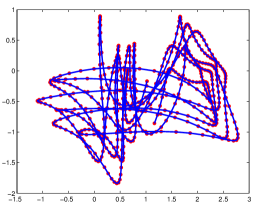
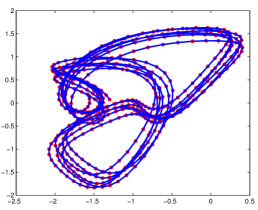
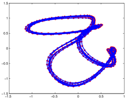
Figure 4: Typical sample paths drawn from the $k_{x(\text{per})}+k_{x(\text{rbf})}$ covariance function. The variances are fixed for the two terms, controlling their relative effect. In Figures 4, 4 and 4, the ratio $\sigma_{\text{rbf}}^{2}/\sigma_{\text{per}}^{2}$ of the two variances was large, intermediate and small respectively, causing the periodic pattern to be shifted proportionally each period.

For our experiments we additionally include a noise covariance function

$$k_{\text{white}}(\mathbf{x}_{i,:},\mathbf{x}_{k,:})=\theta_{\text{white}}\delta_{i,k},$$ (56)

where $\delta_{i,k}$ is the Kronecker delta function. In that way, we can define a compound kernel $k+k_{\text{white}}$, so that the noise level $\theta_{\text{white}}$ can be jointly optimised along with the rest of the kernel hyperparameters. Similarly, one can also include a bias term $\theta_{\text{bias}}\mathbf{1}$.

5.2 Visualisation Tasks

Given a dataset with known structure, we can apply our algorithm and evaluate its performance in a simple and intuitive way, by checking if the form of the discovered low dimensional manifold agrees with our prior knowledge.

We illustrate the method in the multi-phase oil flow data (Bishop and James, 1993) that consists of $1,000$, $12$ dimensional observations belonging to three known classes corresponding to different phases of oil flow. Figure 6 shows the results for these data obtained by applying the variational GP-LVM with $10$ latent dimensions using the exponentiated quadratic ARD kernel. The means of the variational distribution were initialized based on PCA, while the variances in the variational distribution are initialized to neutral values around $0.5$. As shown in Figure 5, the algorithm switches off $8$ out of $10$ latent dimensions by making their inverse lengthscales almost zero. Therefore, the two-dimensional nature of this dataset is automatically revealed. Figure 6 shows the visualization obtained by keeping only the dominant latent directions which are the dimensions $2$ and $3$. This is a remarkably high quality two dimensional visualization of this data. For comparison, Figure 6 shows the visualization provided by the standard sparse GP-LVM that runs by a priori assuming only $2$ latent dimensions. Both models use $50$ inducing variables, while the latent variables $\mathbf{X}$ optimized in the standard GP-LVM are initialized based on PCA. Note that if we were to run the standard GP-LVM with $10$ latent dimensions, the model would overfit the data, it would not reduce the dimensionality in the manner achieved by the variational GP-LVM. The quality of the class separation in the two-dimensional space can also be quantified in terms of the nearest neighbour error; the total error equals the number of training points whose closest neighbour in the latent space corresponds to a data point of a different class (phase of oil flow). The number of nearest neighbour errors made when finding the latent embedding with the standard sparse GP-LVM was $26$ out of $1000$ points, whereas the variational GP-LVM resulted in only one error.

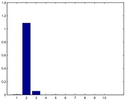
Figure 5: The inverse lengthscales found by applying the variational GP-LVM with ARD EQ kernel on the oil flow data.

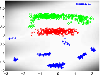
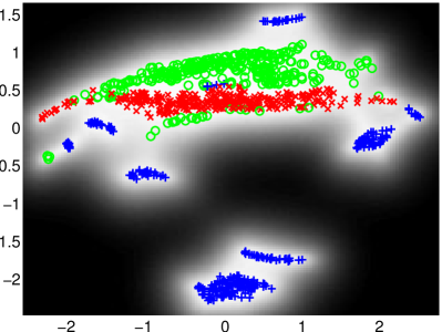
Figure 6: Panel 6 shows the latent space for the variational GP-LVM. Here the dominant latent dimensions are 2 and 3. Dimension 2 is plotted on the $y$-axis and 3 and on the $x$-axis. Plot 6 shows the visualization found by standard sparse GP-LVM initialized with a two dimensional latent space. The nearest neighbor error count for the variational GP-LVM is one. For the standard sparse GP-LVM it is 26.

5.3 Human Motion Capture Data

In this section we consider a data set associated with temporal information, as the primary focus of this experiment is on evaluating the dynamical version of the variational GP-LVM. We followed Taylor et al. (2007); Lawrence (2007) in considering motion capture data of walks and runs taken from subject 35 in the CMU motion capture database. We used the dynamical version of our model and treated each motion as an independent sequence. The data set was constructed and preprocessed as described in (Lawrence, 2007). This results in 2,613 separate 59-dimensional frames split into 31 training sequences with an average length of 84 frames each. Our model does not require explicit timestamp information, since we know a priori that there is a constant time delay between poses and the model can construct equivalent covariance matrices given any vector of equidistant time points.

The model is jointly trained, as explained in the last paragraph of Section 3.3.2, on both walks and runs, i.e. the algorithm learns a common latent space for these motions. At test time we investigate the ability of the model to reconstruct test data from a previously unseen sequence given partial information for the test targets. This is tested once by providing only the dimensions which correspond to the body of the subject and once by providing those that correspond to the legs. We compare with results in (Lawrence, 2007), which used MAP approximations for the dynamical models, and against nearest neighbour. We can also indirectly compare with the binary latent variable model (BLV) of Taylor et al. (2007) which used a slightly different data preprocessing. Furthermore, we additionally tested the non-dynamical version of our model, in order to explore the structure of the distribution found for the latent space. In this case, the notion of sequences or sub-motions is not modelled explicitly, as the non-dynamical approach does not model correlations between datapoints. However, as will be shown below, the model manages to discover the dynamical nature of the data and this is reflected in both, the structure of the latent space and the results obtained on test data.

The performance of each method is assessed by using the cumulative error per joint in the scaled space defined in (Taylor et al., 2007) and by the root mean square error in the angle space suggested by Lawrence (2007). Our models were initialized with nine latent dimensions. For the dynamical version, we performed two runs, once using the Matérn covariance function for the dynamical prior and once using the exponentiated quadratic.

The appropriate latent space dimensionality for the data was automatically inferred by our models. The non-dynamical model selected a $5$-dimensional latent space. The model which employed the Matérn covariance to govern the dynamics retained four dimensions, whereas the model that used the exponentiated quadratic kept only three. The other latent dimensions were completely switched off by the ARD parameters.

From Table 1 we see that the dynamical variational GP-LVM considerably outperforms the other approaches. The best performance for the legs and the body reconstruction was achieved by our dynamical model that used the Matérn and the exponentiated quadratic covariance function respectively. This is an intuitive result, since the smoother body movements are expected to be better modelled using the infinitely differentiable exponentiated quadratic covariance function, whereas the Matérn one can easier fit the rougher leg motion. However, although it is important to take into account any available information about the nature of the data, the fact that both models outperform significantly other approaches shows that the Bayesian training manages successfully to fit the covariance function parameters to the data in any case. Furthermore, the non-dynamical variational GP-LVM, not only manages to discover a latent space with a dynamical structure, as can be seen in Figure 7, but is also proven to be very robust when making predictions. Indeed, Table 1 shows that the non-dynamical variational GP-LVM typically outperforms nearest neighbor and its performance is comparable to the GP-LVM which explicitly models dynamics using MAP approximations. Finally, it is worth highlighting the intuition gained by investigating Figure 7. As can be seen, all models split the encoding for the “walk” and “run” regimes into two subspaces. Further, we notice that the smoother the latent space is constrained to be, the less “circular” is the shape of the “run” regime latent space encoding. This can be explained by noticing the “outliers” in the top left and bottom positions of plot 7. These latent points correspond to training positions that are very dissimilar to the rest of the training set but, nevertheless, a temporally constrained model is forced to accommodate them in a smooth path. The above intuitions can be confirmed by interacting with the model in real time graphically, as is presented in the supplementary video.

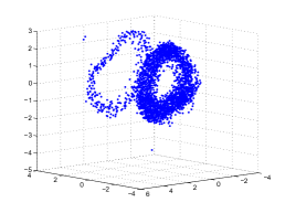
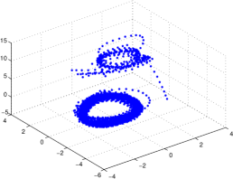
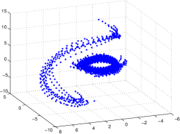
Figure 7: The latent space discovered by our models, projected into its three principle dimensions. The latent space found by the non-dynamical variational GP-LVM is shown in 7, by the dynamical model which uses the Matérn in 7 and by the dynamical model which uses the exponentiated quadratic in 7.

Table 1: Errors obtained for the motion capture dataset considering nearest neighbour in the angle space (NN) and in the scaled space (NN sc.), GP-LVM, BLV, variational GP-LVM (VGP-LVM) and Dynamical Variational GP-LVM (Dyn. VGP-LVM). CL / CB are the leg and body data sets as preprocessed in (Taylor et al., 2007), L and B the corresponding datasets from Lawrence (2007). SC corresponds to the error in the scaled space, as in Taylor et al. while RA is the error in the angle space. The best error per column is in bold.

Data	CL	CB	L	L	B	B
Error Type	SC	SC	SC	RA	SC	RA
BLV	11.7	8.8	-	-	-	-
NN sc.	22.2	20.5	-	-	-	-
GP-LVM (q= 3)	-	-	11.4	3.40	16.9	2.49
GP-LVM (q= 4)	-	-	9.7	3.38	20.7	2.72
GP-LVM (q= 5)	-	-	13.4	4.25	23.4	2.78
NN sc.	-	-	13.5	4.44	20.8	2.62
NN	-	-	14.0	4.11	30.9	3.20
VGP-LVM	-	-	14.22	5.09	18.79	2.79
Dyn. VGP-LVM (Exp. Quadr.)	-	-	7.76	3.28	11.95	1.90
Dyn. VGP-LVM (Matérn 3/2)	-	-	6.84	2.94	13.93	2.24

5.4 Modeling Raw High Dimensional Video Sequences

For this set of experiments we considered video sequences (which are included in the supplementary videos available on-line). Such sequences are typically preprocessed before modeling to extract informative features and reduce the dimensionality of the problem. Here we work directly with the raw pixel values to demonstrate the ability of the dynamical variational GP-LVM to model data with a vast number of features. This also allows us to directly sample video from the learned model.

Firstly, we used the model to reconstruct partially observed frames from test video sequences . For the first video discussed here we gave as partial information approximately 50% of the pixels while for the other two we gave approximately 40% of the pixels on each frame. The mean squared error per pixel was measured to compare with the $k-$nearest neighbour (NN) method, for $k\in(1,..,5)$ (we only present the error achieved for the best choice of $k$ in each case). The datasets considered are the following: firstly, the ‘Missa’ dataset, a standard benchmark used in image processing. This is a 103,680-dimensional video, showing a woman talking for 150 frames. The data is challenging as there are translations in the pixel space. We also considered an HD video of dimensionality $9\times 10^{5}$ that shows an artificially created scene of ocean waves as well as a $230,400-$dimensional video showing a dog running for $60$ frames. The later is approximately periodic in nature, containing several paces from the dog. For the first two videos we used the Matérn and exponentiated quadratic covariance functions respectively to model the dynamics and interpolated to reconstruct blocks of frames chosen from the whole sequence. For the ‘dog’ dataset we constructed a compound kernel $k_{x}=k_{x(\text{rbf})}+k_{x(\text{per})}$ presented in section 5.1, where the exponentiated quadratic (RBF) term is employed to capture any divergence from the approximately periodic pattern. We then used our model to reconstruct the last 7 frames extrapolating beyond the original video. As can be seen in Table 2, our method outperformed NN in all cases. The results are also demonstrated visually in Figures 8, 9, 10 and 11 and the reconstructed videos are available in the supplementary material.

Table 2: The mean squared error per pixel for Dyn. VGP-LVM and NN for the three datasets (measured only in the missing inputs). The number of latent dimensions selected by our model is in parenthesis.

	Missa	Ocean	Dog
Dyn. VGP-LVM	2.52 ($q=12$)	9.36 ($q=9$)	4.01 ($q=6$)
NN	2.63	9.53	4.15

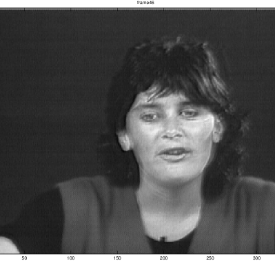
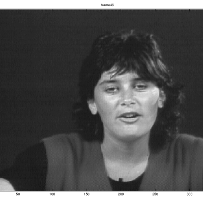
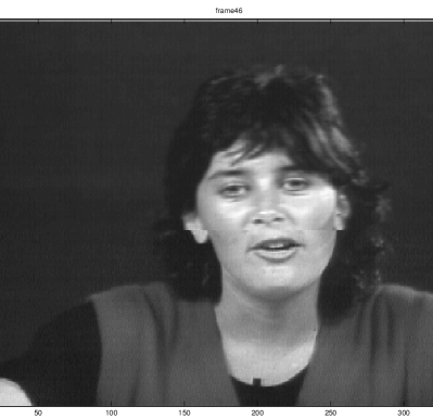
Figure 8: 8 and 8 demonstrate the reconstruction achieved by dynamical variational GP-LVM and NN respectively for one of the most challenging frames 8 of the ‘missa’ video, i.e. when translation occurs. In contrast to the NN method, which works in the whole high dimensional pixel space, our method reconstructed the images using a $12$-dimensional compression for the ‘missa’ video.

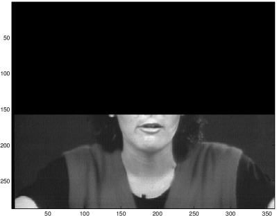
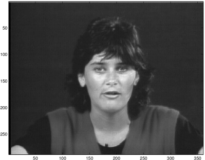
Figure 9: Another example of the reconstruction achieved by the dynamical variational GP-LVM given the partially observed image.

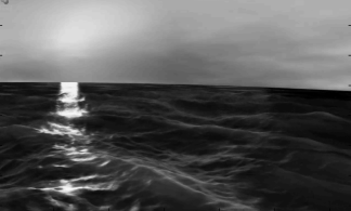
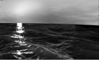
Figure 10: 10 (Dynamical variational GP-LVM) and 10 (NN) depict the reconstruction achieved for a frame of the ‘ocean’ dataset. Notice that in both of the aforementioned datasets, our method recovers a smooth image, in contrast to the simple NN (a close up of this problem with NN for the ‘ocean’ video is shown in Figure 10). The dynamical var. GP-LVM reconstructed the ocean images using a $9$-dimensional compression for the video.

As can be seen in Figures 8, 9 and 10, the dynamical variational GP-LVM predicts pixels which are smoothly connected with the observed part of the image, whereas the NN method cannot fit the predicted pixels in the overall context. Figure 810 focuses on this specific problem with NN, but it can be seen more evidently in the corresponding video files.

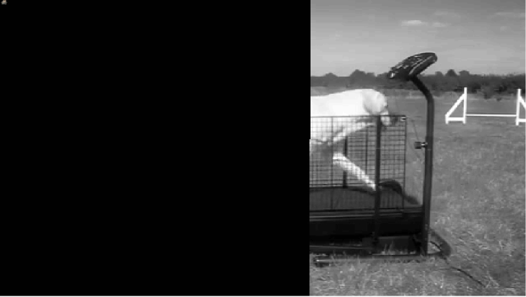
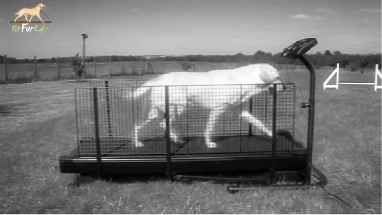
Figure 11: An example for the reconstruction achieved for the ‘dog’ dataset. $40\%$ of the test image’s pixels (Figures 11 were presented to the model, which was able to successfully reconstruct them, as can be seen in 11.

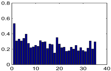
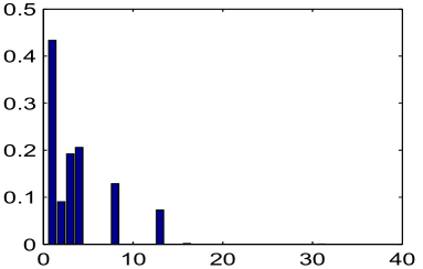
Figure 12: Here, we also demonstrate the ability of the model to automatically select the latent dimensionality by showing the initial lengthscales (fig: 12) of the ARD covariance function and the values obtained after training (fig: 12) on the ‘dog’ data set.

As a second task, we used our generative model to create new samples and generate a new video sequence. This is most effective for the ‘dog’ video as the training examples were approximately periodic in nature. The model was trained on 60 frames (time-stamps $[t_{1},t_{60}]$) and we generated new frames which correspond to the next 40 time points in the future. The only input given for this generation of future frames was the time-stamp vector, $[t_{61},t_{100}]$. The results show a smooth transition from training to test and amongst the test video frames. The resulting video of the dog continuing to run is sharp and high quality. This experiment demonstrates the ability of the model to reconstruct massively high dimensional images without blurring. Frames from the result are shown in Figure 13. The full video is available in the supplementary material.

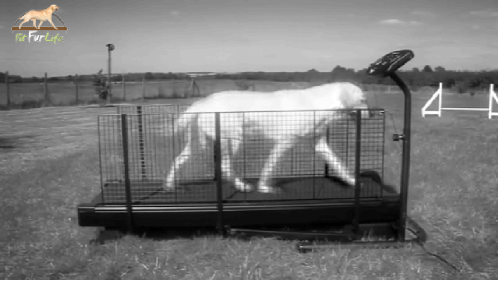
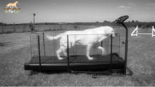
Figure 13: The last frame of the training video 13 is smoothly followed by the first frame 13 of the generated video. A subsequent generated frame can be seen in 13.

5.5 Class Conditional Density Estimation

In this experiment we use the variational GP-LVM to build a generative classifier for handwritten digit recognition. We consider the well known USPS digits dataset. This dataset consists of $16\times 16$ images for all $10$ digits and it is divided into $7,291$ training examples and $2,007$ test examples. We run $10$ variational GP-LVMs, one for each digit, on the USPS data base. We used $10$ latent dimensions and $50$ inducing variables for each model. This allowed us to build a probabilistic generative model for each digit so that we can compute Bayesian class conditional densities in the test data having the form $p(\mathbf{{Y}}_{*}|\mathbf{{Y}},\text{digit})$. These class conditional densities are approximated through the ratio of lower bounds in eq. (44) as described in Section 4. The whole approach allows us to classify new digits by determining the class labels for test data based on the highest class conditional density value and using a uniform prior over class labels. For comparison we used a 1-vs-all logistic regression classification approach. As shown in Table 3, the variational GP-LVM outperforms this baseline.

Table 3: The test error made by the variational GP-LVM and 1-vs-all Logistic Regression classification in the whole set of $2,007$ test points.

	# misclassified	error (%)
variational GP-LVM	$\mathbf{95}$	$\mathbf{4.73}$ %
Logistic Regression	$283$	$14.10$ %

6 Extensions for Different Kinds of Inputs

So far we considered the typical dimensionality reduction scenario where, given high-dimensional output data we seek to find a low-dimensional latent representation in a completely unsupervised manner. For the dynamical variational GP-LVM we have additional temporal information, but the input space $\mathbf{{X}}$ from where we wish to propagate the uncertainty is still treated as fully unobserved. However, our framework for propagating the input uncertainty through the GP mapping is applicable to the full spectrum of cases, ranging from fully unobserved to fully observed inputs with known or unknown amount of uncertainty per input. In this section we discuss these cases and, further, show how they give rise to an auto-regressive model (Section 6.1) and a semi-supervised GP model (Section 6.2).

6.1 Gaussian Process Inference with Uncertain Inputs

Gaussian processes have been used extensively and with great success in a variety of regression tasks. In the most common setting, we are given a dataset of observed input-output pairs, denoted as $\mathbf{Z}\in\Re^{n\times q}$ and $\mathbf{{Y}}\in\Re^{n\times p}$ respectively, and we wish to infer the unknown outputs $\mathbf{{Y}}^{*}\in\Re^{n^{*}\times p}$ corresponding to some novel given inputs $\mathbf{Z}^{*}\in\Re^{n^{*}\times q}$. However, in many real-world applications the inputs are uncertain, for example when measurements come from noisy sensors. In this case, the GP methodology cannot be trivially extended to account for the variance associated with the input space (Girard et al., 2003; McHutchon and Rasmussen, 2011). The aforementioned problem is also closely related to the field of heteroscedastic Gaussian process regression, where the uncertainty in the noise levels is modelled in the output space as a function of the inputs (Kersting et al., 2007; Goldberg et al., 1998; Lázaro-Gredilla and Titsias, 2011).

In this section we show that our variational framework can be used to explicitly model the input uncertainty in the GP regression setting. The assumption made is that the observed inputs $\mathbf{Z}$ are obtained by the noise-free latent inputs $\mathbf{{X}}$ by adding Gaussian noise,

$$\mathbf{z}_{i,:}=\mathbf{x}_{i,:}+\bm{\epsilon}_{x},$$ (57)

where $\mathbf{z}_{i,:}$ denotes the $i$-th observed input of the dataset $\mathbf{Z}$ and $\bm{\epsilon}_{z}\sim\mathcal{N}\left(\mathbf{0},\bm{\Sigma}_{z}\right)$, as in (McHutchon and Rasmussen, 2011). Since $\mathbf{Z}$ is observed and $\mathbf{{X}}$ unobserved the above equation essentially induces a Gaussian prior distribution over $\mathbf{{X}}$ that has the form,

$$p(\mathbf{{X}}|\mathbf{Z})=\prod_{i=1}^{n}\mathcal{N}\left(\mathbf{x}_{i,:}|\mathbf{z}_{i,:},\bm{\Sigma}_{z}\right),$$ (58)

where $\bm{\Sigma}_{z}$ is typically an unknown parameter. Given that $\mathbf{{X}}$ are really the inputs that eventually are passed through the GP latent function (to subsequently generate the outputs) the whole probabilistic model becomes a GP-LVM with the above special form for the prior distribution over the latent inputs, making thus our variational framework easily applicable. More precisely, using the above prior, we can define a variational bound on $p(\mathbf{{Y}})$ as well as an associated approximation $q(\mathbf{{X}})$ to the true posterior $p(\mathbf{{X}}|\mathbf{{Y}},\mathbf{Z})$. This variational distribution $q(\mathbf{{X}})$ can be used as a probability estimate of the noisy input locations $\mathbf{{X}}$. During optimisation of the lower bound we can also learn the parameter $\bm{\Sigma}_{z}$. Furthermore, if we wish to reduce the number of parameters in the variational distribution $q(\mathbf{{X}})=\mathcal{N}\left(\mathcal{M},\mathcal{S}\right)$ a sensible choice would be to set $\mathcal{M}=\mathbf{Z}$, although such a choice may not be optimal.

Having a method which implicitly models the uncertainty in the inputs also allows for doing predictions in an autoregressive manner while propagating the uncertainty through the predictive sequence (Girard et al., 2003). To demonstrate this in the context of our framework, we will take the simple case where the process of interest is a multivariate time-series given as pairs of time points $\mathbf{t}=\{t\}_{i=1}^{n}$ and corresponding output locations $\mathbf{{Y}}=\{\mathbf{y}_{i,:}\}_{i=1}^{n}$, $\mathbf{y}_{i,:}\in\Re^{p}$. Here, we take the time locations to be deterministic and equally spaced, so that they can be simply denoted by the subscript of the output points $\mathbf{y}_{i,:}$; we thus simply denote with $\mathbf{y}_{k}$ the output point $\mathbf{y}_{k,:}$ which corresponds to $t_{k}$.

We can now reformat the given data $\mathbf{{Y}}$ into input-output pairs $\hat{\mathbf{Z}}$ and $\hat{\mathbf{{Y}}}$, where:

$$[\hat{\mathbf{z}}_{1},\hat{\mathbf{z}}_{2},...,\hat{\mathbf{z}}_{n-\tau}] =\left[\left[\mathbf{y}_{1},\mathbf{y}_{2},...,\mathbf{y}_{\tau}\right],\left[\mathbf{y}_{2},\mathbf{y}_{3},...,\mathbf{y}_{\tau+1}\right],...,\left[\mathbf{y}_{n-\tau},\mathbf{y}_{n-\tau+1},...,\mathbf{y}_{n-1}\right]\right],$$

$$[\hat{\mathbf{y}}_{1},\hat{\mathbf{y}}_{2},...,\hat{\mathbf{y}}_{n-\tau}] =[\mathbf{y}_{\tau+1},\mathbf{y}_{\tau+2},...,\mathbf{y}_{n}]$$

and $\tau$ is the size of the dynamics’ “memory”. In other words, we define a window of size $\tau$ which shifts in time so that the output in time $t$ becomes an input in time $t+1$. Therefore, the uncertain inputs method described earlier in this section can be applied to the new dataset $[\hat{\mathbf{Z}},\hat{\mathbf{{Y}}}]$. In particular, although the training inputs $\hat{\mathbf{Z}}$ are not necessarily uncertain in this case, the aforementioned way of performing inference is particularly advantageous when the task is extrapolation.

In more detail, consider the simplest case described in this section where the posterior $q(\mathbf{{X}})$ is centered in the given noisy inputs and we allow for variable noise around the centers. To perform extrapolation one firstly needs to train the model on the dataset $[\hat{\mathbf{Z}},\hat{\mathbf{{Y}}}]$. Then, we can perform iterative $k-$step ahead prediction in order to find a future sequence $\left[\mathbf{y}_{n+1},\mathbf{y}_{n+2},...\right]$ where, similarly to the approach taken by Girard et al. (2003), the predictive variance in each step is accounted for and propagated in the subsequent predictions. For example, if $k=1$ the algorithm will make iterative 1-step predictions in the future; in the beginning, the output $\mathbf{y}_{n+1}$ will be predicted given the training set. In the next step, the training set will be augmented to include the previously predicted $\mathbf{y}_{n+1}$ as part of the input set, where the predictive variance is now encoded as the uncertainty of this point.

The advantage of the above method, which resembles a state-space model, is that the future predictions do not almost immediately revert to the mean, as in standard stationary GP regression, neither do they underestimate the uncertainty, as would happen if the predictive variance was not propagated through the inputs in a principled way.

6.1.1 Demonstration: iterative $k-$step ahead forecasting

Here we demonstrate our framework in the simulation of a state space model, as was described previously. More specifically, we consider the Mackey-Glass chaotic time series, a standard benchmark which was also considered in (Girard et al., 2003). The data is one-dimensional so that the timeseries can be represented as pairs of values $\{\mathbf{y},\mathbf{t}\},t=1,2,\cdots,n$ and simulates:

$$\frac{\text{d}\zeta(t)}{dt}=-b\zeta(t)\alpha\frac{\zeta(t-T)}{1+\zeta(t-T)^{10}},\;\;\text{with}\;\;\alpha=0.2,b=0.1,T=17.$$

As can be seen, the generating process is very non-linear, something which makes this dataset particularly challenging.

The model trained on this dataset was the one described previously, where the modified dataset $\{\hat{\mathbf{y}},\hat{\mathbf{z}}\}$ was created with $\tau=16$ and we used the first $96$ points to train the model and predicted the subsequent $180$ points in the future. The comparison was made firstly with a standard GP model (which we refer to as $\mathcal{GP}_{\mathbf{t},\mathbf{y}}$), where the input - output pairs were given in the standard form, that is, $\mathbf{t}$ and $\mathbf{y}$ respectively and the predictions were made in the standard way, that is, given $\mathbf{t}_{*}$. Further, we compared with a standard GP model where the input - output pairs were given by the modified dataset $\{\hat{\mathbf{z}},\hat{\mathbf{y}}\}$ that was mentioned previously; this model is here referred to as $\mathcal{GP}_{\hat{\mathbf{z}},\hat{\mathbf{y}}}$. For the latter model, the predictions are made in the $k-$step ahead manner, according to which the predicted values for iteration $k$ are added to the training set. However, this standard GP model has no straight forward way of propagating the uncertainty, and therefore the input uncertainty is zero for every step of the iterative predictions.

The predictions obtained can be seen in Figure 14.

Figure 14: Iterative $1-$step ahead prediction for a chaotic timeseries. Comparing a standard GP approach ($\mathcal{GP}_{\mathbf{t},\mathbf{y}}$), an “autoregressive” GP approach which does not propagate uncertainties ($\mathcal{GP}_{\hat{\mathbf{z}},\hat{\mathbf{y}}}$) and the variational GP-LVM (VGPLVM) in an “autoregressive” setting.

As can be seen, the variational GP-LVM is more robust in handling the uncertainty throughout the predictions something which results in lower predictive error. In particular, notice that in the first few predictions all methods give the same answer. However, the standard GP regression model, $\mathcal{GP}_{\mathbf{t},\mathbf{y}}$, very quickly reverts to the mean, as expected, when the test inputs are too far from the training ones and the uncertainty is very large. On the other hand, $\mathcal{GP}_{\hat{\mathbf{z}},\hat{\mathbf{y}}}$ has the opposite problem; every predictive step results in a prediction which underestimates the uncertainty; therefore, although the initial predictions are reasonable, once they diverge a little by the true values the error is carried on and amplified.

6.2 Semi-supervised GP Regression and Data Imputation

In this section, we describe how our proposed model can be used in a data imputation / semi-supervised regression problem where part of the training inputs are missing. This scenario is obviously a special case of the uncertain input modeling discussed above. Although a more general setting can be defined, here we consider the case where we have a fully and a partially observed set of inputs, i.e. $\mathbf{Z}=(\mathbf{Z}^{o},\mathbf{Z}^{u})$, where $o$ and $u$ denote set of rows of $(\mathbf{Z},\mathbf{{Y}})$ that contain fully and partially observed inputs respectively. This is a realistic scenario; it is often the case that certain input features are more difficult to obtain (e.g. human specified tags) than others, but we would nevertheless wish to model all available information within the same model. The features missing in $\mathbf{Z}^{u}$ can be different in number / location for each individual point $\mathbf{z}^{u}_{i,:}$.

A standard GP regression model cannot straightforwardly model jointly $\mathbf{Z}^{o}$ and $\mathbf{Z}^{u}$. In contrast, in our framework the inputs are replaced by distributions $q(\mathbf{{X}}^{o})$ and $q(\mathbf{{X}}^{u})$, so that $\mathbf{Z}^{u}$ can be taken into account naturally by simply initialising the uncertainty of $q(\mathbf{{X}}^{u})$ in the missing locations to 1 (assuming normalized inputs) and the mean to the empirical mean and then, optionally, optimising $q(\mathbf{{X}}^{u})$. In our experiments we use a slightly more sophisticated approach which resulted in better results. Specifically, we can use the fully observed data subset $(\mathbf{Z}^{o},\mathbf{{Y}}^{o})$ to train an initial model for which we fix $q(\mathbf{{X}}^{o})=\mathcal{N}\left(\mathbf{{X}}^{o}|\mathbf{Z}^{o},\mathbf{0}\right)$. Given this model, we can then use $\mathbf{{Y}}^{u}$ to estimate the predictive posterior $q(\mathbf{{X}}^{u}$) in the missing locations of $\mathbf{Z}^{u}$ (for the observed locations we match the mean with the observations, as for $\mathbf{Z}^{o}$). After initializing $q(\mathbf{{X}})=q(\mathbf{{X}}^{o},\mathbf{{X}}^{u})$ in this way, we can proceed by training our model on the full (extended) training set $\left(\left(\mathbf{Z}^{o},\mathbf{Z}^{u}\right),\left(\mathbf{{Y}}^{o},\mathbf{{Y}}^{u}\right)\right)$, which contains fully and partially observed inputs. During this training phase, the variational distribution $q(\mathbf{{X}})$ is held fixed in the locations corresponding to observed values and is optimised in the locations of missing inputs.

Given the above formulation, we can define a semi-supervised GP model which naturally incorporates fully and partially observed examples by communicating the uncertainty throughout the relevant parts of the model in a principled way. In specific, the predictive uncertainty obtained by the initial model trained on the fully observed data can be incorporated as input uncertainty via $q(\mathbf{{X}}^{u})$ in the model trained on the extended dataset, similarly to how extrapolation was achieved for our auto-regressive approach in Section 6.1. In extreme cases resulting in very non-confident predictions, for example presence of outliers, the corresponding locations will simply be ignored automatically due to the large uncertainty. This mechanism, together with the subsequent optimisation of $q(\mathbf{{X}}^{u})$, guards against reinforcing bad predictions when imputing missing values based on a smaller training set. In particular, in the limit of having no observed values the semi-supervised GP is equivalent to the GP-LVM and when there are no missing values (or when all missing locations have uncertainty $1$) it is equivalent to GP regression. Details of the algorithm for this approach are given in Appendix E.

The algorithm defined above can be seen as a particular instance of semi-supervised learning which uses self-training for initialisation. Traditionally, semi-supervised settings are encountered in classification problems where only part of the training data are associated with known class labels. A simple approach to exploiting the unlabelled examples is to use self-training (Rosenberg et al., 2005), according to which an initial model is trained on the labelled examples and then used to incorporate the unlabelled examples in the manner dictated by the specific self-training methodology followed. In a bootstrap-based self-training approach this incoroporation is achieved by predicting the missing labels using the initial model and, subsequently, augmenting the training set using only the confident predictions subset. Recently, Kingma et al. (2014) demonstrated the applicability of generative models in semi-supervised learning. Their method defines a latent space $\mathbf{{X}}$ and estimates an approximate and factorised with respect to data points posterior $q(\mathbf{{X}}|\mathbf{Z})$ using labelled and unlabelled examples. Subsequently, the algorithm builds a classifier from the latent to the label space by sampling from areas of the approximate posterior that correspond to labelled instances.

While our framework can be adapted to tackle the aforementioned classification scenario, this is redirected to future work. Instead, here we focused on a regression problem where the missing values appear in the inputs. However, there exist some similarities with the work referenced in the previous paragraph. In specific, our generative method treats the semi-supervised task as a data imputation problem, similarly to (Kingma et al., 2014). One of the differences with their work is that we do not use a latent space representation for the inputs but, instead, we directly associate the input space with uncertainty. Concerning relations with other methods which use self-training, our algorithm also trains an initial model on the fully observed portion of the data and predicts the missing values. However, these predictions only constitute initialisations which are later optimised along with model parameters and, hence, we refer to this step as partial self-training. Further, in our framework the predictive uncertainty is not used as a hard measure of discarding unconfident predictions but, instead, we allow all values to contribute according to an optimised uncertainty measure. Therefore, the way in which uncertainty is handled makes the self-training part of our algorithm principled compared to many bootstrap-based approaches.

6.2.1 Demonstration

In this section we consider simulated and real-world data to demonstrate our semi-supervised GP algorithm, which was discussed in Section 6.2. The simulated data were created by sampling inputs $\mathbf{Z}$ from an unknown to the competing models GP and gave this as input to another (again, unknown) GP to obtain the corresponding outputs $\mathbf{{Y}}$. For the real-world data demonstration we considered a subset of the same motion capture dataset discussed in Section 5.3, which corresponds to a walking motion of a human body represented as a set of $59$ joint locations. We formulated a regression problem where the first $20$ dimensions of the original data are used as targets and the rest $39$ as inputs. In other words, given a partial joint representation of the human body, the task is to infer the rest of the representation. For both datasets, simulated and motion capture, we selected a portion of the training inputs, denoted as $\mathbf{Z}^{u}$, to have randomly missing features. The extended dataset $\left(\left(\mathbf{Z}^{o},\mathbf{Z}^{u}\right),\left(\mathbf{{Y}}^{o},\mathbf{{Y}}^{u}\right)\right)$ was used to train our method as well as multiple linear regression (MLR). Using only the observed data $\left(\mathbf{Z}^{o},\mathbf{{Y}}^{o}\right)$ we trained a standard GP and nearest neighbour (NN), both of which cannot handle missing inputs straightforwardly. The goal was to reconstruct test outputs $\mathbf{{Y}}_{*}$ given fully observed test inputs $\mathbf{Z}_{*}$. For the simulated data we used the following sizes: $|\mathbf{Z}^{o}|=40$, $|\mathbf{Z}^{u}|=60$ and $|\mathbf{Z}_{*}|=100$. The dimensionality of the inputs is $15$ and of the outputs is $5$. For the motion capture data we used $|\mathbf{Z}^{o}|=50$, $|\mathbf{Z}^{u}|=80$ and $|\mathbf{Z}_{*}|=200$. In Figure 15 we plot the MSE obtained by the competing methods for a varying percentage of missing features in $\mathbf{Z}^{u}$. For the simulated data experiment, each of the points in the plot is an average of 4 runs which considered different random seeds. As can be seen, the semi-supervised GP is able to handle the extra data and make better predictions, even if a very large portion is missing. Indeed, its performance starts to converge to that of a standard GP when there are 90% missing values in $\mathbf{Z}^{u}$ and performs identically to the standard GP when 100% of the values are missing.

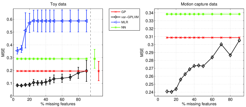
Figure 15: Mean Squared Error for predictions obtained by different methods in simulated (left) and motion capture data (right). Flat line errors correspond to methods that cannot take into account partially observed inputs. The results for simulated data are obtained from 4 trials and, hence, errorbars are also plotted. For GP and NN, errorbars do not change with $x$-axis and, for clarity, they are plotted separately on the right of the dashed vertical line (for nonsensical $x$ values). Methods that resulted in very high MSE compared to the rest are not shown, for clearer plots; specifically, MSE for predicting with the data mean was $0.82$. For the motion capture data, MLR performed very badly, with average MSE $0.72$.

7 Conclusion

We have introduced an approximation to the marginal likelihood of the Gaussian process latent variable model in the form of a variational lower bound. This provides a Bayesian training procedure which is robust to overfitting and allows for the appropriate dimensionality of the latent space to be automatically determined. Our framework is extended for the case where the observed data constitute multivariate timeseries and, therefore, we obtain a very generic method for dynamical systems modelling able to capture complex, non-linear correlations. We demonstrated the advantages of the rigorous lower bound defined in our framework on a range of disparate real world data sets. This also emphasised the ability of the model to handle vast dimensionalities.

Our approach was easily extended to be applied to training Gaussian processes with uncertain inputs where these inputs have Gaussian prior densities. This gave rise to an auto-regressive and a semi-supervised GP variant of our model. For future research, we envisage several other extensions that become computationally feasible using the same set of methodologies we espouse. In particular, propagation of uncertain inputs through the Gaussian process allows Bayes filtering (Ko and Fox, 2009a; Deisenroth et al., 2012; Frigola et al., 2014) applications to be carried out through variational bounds. Bayes filters are non-linear dynamical systems where time is discrete and the observed data $\mathbf{y}_{t}$ at time point $t$, is non-linearly related to some unobserved latent state, $\mathbf{x}_{t}$,

$$\mathbf{y}_{t}=f(\mathbf{x}_{t})$$

which itself has a non-linear autoregressive relationship with past latent states:

$$\mathbf{x}_{t}=g(\mathbf{x}_{t-1})$$

where both $g(\cdot)$ and $f(\cdot)$ are assumed to be Gaussian processes. Propagation of the uncertainty through both processes can be achieved through our variational lower bound allowing fast efficient approximations to Gaussian process dynamical models.

The bound also allows for a promising new direction of research, that of deep Gaussian processes. In a deep Gaussian process (Lawrence and Moore, 2007; Damianou and Lawrence, 2013) the idea of placing a temporal prior over the inputs to a GP is further extended by hierarchical application. This formalism leads to a powerful class of models where Gaussian process priors are placed over function compositions, for example in a five layer model we have

$$f(\mathbf{{X}})=g_{5}(g_{4}(g_{3}(g_{2}(g_{1}(\mathbf{{X}})))))$$

where each $g_{i}(\cdot)$ is a draw from a Gaussian process. By combining such models with structure learning (Damianou et al., 2012) we can develop the potential to learn very complex non linear interactions between data. In contrast to other deep models all the uncertainty in parameters and latent variables is marginalised out.

Acknowledgments

This research was partially funded by the European research project EU FP7-ICT (Project Ref 612139 “WYSIWYD”), the Greek State Scholarships Foundation (IKY) and the University of Sheffield Moody endowment fund. We also thank Colin Litster and “Fit Fur Life” for allowing us to use their video files as datasets.

A Further Details About the Variational Bound

This appendix contains supplementary details for deriving some mathematical formulae related to the calculation of the final expression of the variational lower bound for the training phase.

Since many derivations require completing the square to recognize a Gaussian, we will use the following notation throughout the Appendix:

$$\mathcal{Z}=\text{the collection of all constants for the specific line in equation},$$

where the definition of a constant depends on the derivation at hand.

A.1 Calculation of: $\left\langle\log p(\mathbf{y}_{:,j}|\mathbf{f}_{:,j})\right\rangle_{p(\mathbf{f}_{:,j}|\mathbf{u}_{:,j},\mathbf{{X}})}$

First, we show in detail how to obtain the r.h.s of equation (25) for the following quantity:
$\left\langle\log p(\mathbf{y}_{:,j}|\mathbf{f}_{:,j})\right\rangle_{p(\mathbf{f}_{:,j}|\mathbf{u}_{:,j},\mathbf{{X}})}$ which appears in the variational bound of equation (24). Notice that this term itself lower bounds the logarithm of the likelihood:

$$\log p(\mathbf{y}_{:,j}|\mathbf{{X}}) =\log\int p(\mathbf{y}_{:,j}|\mathbf{f}_{:,j})p(\mathbf{f}_{:,j}|\mathbf{u}_{:,j},\mathbf{{X}})\text{d}\mathbf{f}_{:,j}\text{d}\mathbf{u}_{:,j}$$

$$\geq\int p(\mathbf{f}_{:,j}|\mathbf{u}_{:,j},\mathbf{{X}})\log p(\mathbf{y}_{:,j}|\mathbf{f}_{:,j})\text{d}\mathbf{f}_{:,j}\text{d}\mathbf{u}_{:,j},$$ (59)

where the last line follows from Jensen’s inequality. In the following, we compute the above quantity analytically while temporarily using the notation $\left\langle\cdot\right\rangle=\left\langle\cdot\right\rangle_{p(\mathbf{f}_{:,j}|\mathbf{u}_{:,j},\mathbf{{X}})}$ :

$$\left\langle\log p(\mathbf{y}_{:,j}|\mathbf{f}_{:,j})\right\rangle\stackrel{{\scriptstyle\text{eq. }\eqref{eq:yGivenF}}}{{=}}{} \left\langle\log\mathcal{N}\left(\mathbf{y}_{:,j}|\mathbf{f}_{:,j},\sigma^{2}\mathbf{I}_{p}\right)\right\rangle$$

$$={} -\frac{n}{2}\log(2\pi)-\frac{1}{2}\log|\sigma^{2}\mathbf{I}_{p}|-\frac{1}{2}\text{tr}\left(\sigma^{-2}\mathbf{I}_{p}\left(\mathbf{y}_{:,j}\mathbf{y}_{:,j}^{\top}-2\mathbf{y}_{:,j}\left\langle\mathbf{f}_{:,j}^{\top}\right\rangle+\left\langle\mathbf{f}_{:,j}\mathbf{f}_{:,j}^{\top}\right\rangle\right)\right)$$

$$\stackrel{{\scriptstyle\text{eq. }\eqref{priorF2}}}{{=}}{} \mathcal{Z}-\frac{1}{2}\text{tr}\left(\sigma^{-2}\mathbf{I}_{p}\left(\mathbf{y}_{:,j}\mathbf{y}_{:,j}^{\top}-2\mathbf{y}_{:,j}\mathbf{a}_{j}^{\top}+\mathbf{a}_{j}\mathbf{a}_{j}^{\top}+\bm{\Sigma}_{f}\right)\right).$$

By completing the square we find:

$$\left\langle\log p(\mathbf{y}_{:,j}|\mathbf{f}_{:,j})\right\rangle_{p(\mathbf{f}_{:,j}|\mathbf{u}_{:,j},\mathbf{{X}})}={} \log\mathcal{N}\left(\mathbf{y}_{:,j}|\mathbf{a}_{j},\sigma^{2}\mathbf{I}_{p}\right)-\frac{1}{2}\text{tr}\left(\sigma^{-2}\bm{\Sigma}_{f}\right)$$

$$\stackrel{{\scriptstyle\text{eq. }\eqref{eq:conditionalGPmeanCovar}}}{{=}}{} \log\mathcal{N}\left(\mathbf{y}_{:,j}|\mathbf{a}_{j},\sigma^{2}\mathbf{I}_{p}\right)-\frac{1}{2\sigma^{2}}\text{tr}\left(\mathbf{{K}}_{ff}-\mathbf{{K}}_{fu}\mathbf{{K}}_{uu}^{-1}\mathbf{{K}}_{uf}\right).$$ (60)

A.2 Calculating the Explicit Form of $q(\mathbf{u}_{:,j})$

From equation (27), we have:

$$\log q(\mathbf{u}_{:,j})\propto\left\langle\log\mathcal{N}\left(\mathbf{y}_{:,j}|\mathbf{a}_{j},\sigma^{2}\mathbf{I}_{p}\right)\right\rangle_{q(\mathbf{{X}})}+\log p(\mathbf{u}_{:,j}).$$ (61)

All the involved distributions are Gaussian and, hence, we only need to compute the r.h.s of the above equation and complete the square in order to get the posterior Gaussian distribution for $q(\mathbf{u}_{:,j})$. The expectation appearing in the above equation is easily computed as:

$$\left\langle\log\mathcal{N}\left(\mathbf{y}_{:,j}|\mathbf{a}_{j},\sigma^{2}\mathbf{I}_{p}\right)\right\rangle_{q(\mathbf{{X}})}= \mathcal{Z}-\frac{1}{2\sigma^{2}}\text{tr}\left(\mathbf{y}_{:,j}\mathbf{y}_{:,j}^{\top}-2\mathbf{y}_{:,j}\left\langle\mathbf{a}_{j}^{\top}\right\rangle_{q(\mathbf{{X}})}+\left\langle\mathbf{a}_{j}\mathbf{a}_{j}^{\top}\right\rangle_{q(\mathbf{{X}})}\right)$$

$$\stackrel{{\scriptstyle\text{eq. }\eqref{eq:conditionalGPmeanCovar}}}{{=}} \mathcal{Z}-\frac{1}{2\sigma^{2}}\text{tr}\Big{(}\mathbf{y}_{:,j}\mathbf{y}_{:,j}^{\top}-2\mathbf{y}_{:,j}\mathbf{u}_{:,j}^{\top}\mathbf{{K}}_{uu}^{-1}\left\langle\mathbf{{K}}_{fu}^{\top}\right\rangle_{q(\mathbf{{X}})}$$

$$\quad\;\;\qquad+\mathbf{u}_{:,j}^{\top}\mathbf{{K}}_{uu}^{-1}\left\langle\mathbf{{K}}_{fu}^{\top}\mathbf{{K}}_{fu}\right\rangle_{q(\mathbf{{X}})}\mathbf{{K}}_{uu}^{-1}\mathbf{u}_{:,j}\Big{)}$$

$$\stackrel{{\scriptstyle\text{eq. }\eqref{psis}}}{{=}} \mathcal{Z}-\frac{1}{2\sigma^{2}}\text{tr}\Big{(}\mathbf{y}_{:,j}\mathbf{y}_{:,j}^{\top}-2\mathbf{y}_{:,j}\mathbf{u}_{:,j}^{\top}\mathbf{{K}}_{uu}^{-1}\bm{\Psi}_{1}^{\top}$$

$$\quad\;\;\qquad+\mathbf{u}_{:,j}^{\top}\mathbf{{K}}_{uu}^{-1}\bm{\Psi}_{2}\mathbf{{K}}_{uu}^{-1}\mathbf{u}_{:,j}\Big{)}.$$ (62)

We can now easily find equation (61) by combining equations (62) and (20):

$$\log q(\mathbf{u}_{:,j}) \propto\left\langle\log\mathcal{N}\left(\mathbf{y}_{:,j}|\mathbf{a}_{j},\sigma^{2}\mathbf{I}_{p}\right)\right\rangle_{q(\mathbf{{X}})}+\log p(\mathbf{u}_{:,j})$$

$$=\mathcal{Z}-\frac{1}{2\sigma^{2}}\text{tr}\Big{(}\mathbf{y}_{:,j}\mathbf{y}_{:,j}^{\top}-2\mathbf{y}_{:,j}\mathbf{u}_{:,j}^{\top}\mathbf{{K}}_{uu}^{-1}\bm{\Psi}_{1}^{\top}+\mathbf{u}_{:,j}^{\top}\mathbf{{K}}_{uu}^{-1}\bm{\Psi}_{2}\mathbf{{K}}_{uu}^{-1}\mathbf{u}_{:,j}\Big{)}$$

$$\qquad\;\;\;\qquad-\frac{1}{2}\text{tr}\Big{(}\mathbf{{K}}_{uu}^{-1}\mathbf{u}_{:,j}\mathbf{u}_{:,j}^{\top}\Big{)}$$

$$=\mathcal{Z}-\frac{1}{2}\text{tr}\Big{(}\mathbf{u}_{:,j}^{\top}\left(\sigma^{-2}\mathbf{{K}}_{uu}^{-1}\bm{\Psi}_{2}\mathbf{{K}}_{uu}^{-1}+\mathbf{{K}}_{uu}^{-1}\right)\mathbf{u}_{:,j}+\sigma^{-2}\mathbf{y}_{:,j}\mathbf{y}_{:,j}^{\top}-2\sigma^{-2}\mathbf{{K}}_{uu}^{-1}\bm{\Psi}_{1}^{\top}\mathbf{y}_{:,j}\mathbf{u}_{:,j}^{\top}\Big{)}.$$ (63)

We can now complete the square again and recognize that $q(\mathbf{u}_{:,j})=\mathcal{N}\left(\mathbf{u}_{:,j}|\bm{\mu}_{u},\bm{\Sigma}_{u}\right)$, where:

$$\bm{\Sigma}_{u}={} \left(\sigma^{-2}\mathbf{{K}}_{uu}^{-1}\bm{\Psi}_{2}\mathbf{{K}}_{uu}^{-1}+\mathbf{{K}}_{uu}^{-1}\right)^{-1}\mbox{\;\;\;\; and}$$

$$\bm{\mu}_{u}={} \sigma^{-2}\bm{\Sigma}_{u}\mathbf{{K}}_{uu}^{-1}\bm{\Psi}_{1}^{\top}\mathbf{y}_{:,j}.$$

By “pulling” the $\mathbf{{K}}_{uu}$ matrices out of the inverse and after simple manipulations we get the final form of $q(\mathbf{u}_{:,j})$:

$$q(\mathbf{u}_{:,j})={} \mathcal{N}\left(\mathbf{u}_{:,j}|\bm{\mu}_{u},\bm{\Sigma}_{u}\right)\mbox{\;\; where}$$ (64)

$$\bm{\mu}_{u}={} \mathbf{{K}}_{uu}\left(\sigma^{2}\mathbf{{K}}_{uu}+\bm{\Psi}_{2}\right)^{-1}\bm{\Psi}_{1}^{\top}\mathbf{y}_{:,j}$$

$$\bm{\Sigma}_{u}={} \sigma^{2}\mathbf{{K}}_{uu}\left(\sigma^{2}\mathbf{{K}}_{uu}+\bm{\Psi}_{2}\right)^{-1}\mathbf{{K}}_{uu}.$$

A.3 Detailed Derivation of $\hat{\mathcal{F}}_{j}(q(\mathbf{{X}}))$

The quantity $\hat{\mathcal{F}}_{j}(q(\mathbf{{X}}))$ appears in equation (28). Based on the derivations of the previous section, we can rewrite equation (63) as a function of the optimal $q(\mathbf{u}_{:,j})$ found in equation (64) by completing the constant terms:

$$\left\langle\log\mathcal{N}\left(\mathbf{y}_{:,j}|\mathbf{a}_{j},\sigma^{2}\mathbf{I}_{p}\right)\right\rangle_{q(\mathbf{{X}})}+\log p(\mathbf{u}_{:,j}) =\mathcal{B}+\log\mathcal{N}\left(\mathbf{u}_{d}|\bm{\mu}_{u},\bm{\Sigma}_{u}\right)$$ (65)

where we have defined:

$$\mathcal{B}=-\frac{n}{2}\log(2\pi)-\frac{1}{2}\log|\sigma^{2}\mathbf{I}_{p}|-\frac{1}{2}\log|\mathbf{{K}}_{uu}|-\frac{1}{2\sigma^{2}}\mathbf{y}_{:,j}^{\top}\mathbf{y}_{:,j}+\frac{1}{2}\bm{\mu}_{u}^{\top}\bm{\Sigma}_{u}^{-1}\bm{\mu}_{u}+\frac{1}{2}\log|\bm{\Sigma}_{u}|.$$ (66)

We can now obtain the final expression for (28) by simply putting the quantity of (65) on the exponent and integrating. By doing so, we get:

$$\int e^{\left\langle\log\mathcal{N}\left(\mathbf{y}_{:,j}|\mathbf{a}_{d},\sigma^{2}I_{d}\right)\right\rangle_{q(\mathbf{{X}})}}p(\mathbf{u}_{d})\text{d}\mathbf{u}_{d}=\int e^{\mathcal{B}}e^{\log\mathcal{N}\left(\mathbf{u}_{d}|\bm{\mu}_{u},\bm{\Sigma}_{u}\right)}\text{d}\mathbf{u}_{d}=e^{\mathcal{B}}$$

$$\stackrel{{\scriptstyle\text{eq. }\eqref{eq:boundBterm}}}{{=}}{} \;\;\;\;(2\pi)^{-\frac{N}{2}}\sigma^{-n}|\mathbf{{K}}_{uu}|^{-\frac{1}{2}}e^{-\frac{1}{2\sigma^{2}}\mathbf{y}_{:,j}^{\top}\mathbf{y}_{:,j}}|\bm{\Sigma}_{u}|^{\frac{1}{2}}e^{\frac{1}{2}\bm{\mu}_{u}^{\top}\bm{\Sigma}_{u}^{-1}\bm{\mu}_{u}}.$$ (67)

By using equation (64) and some straightforward algebraic manipulations, we can replace in the above $\bm{\mu}_{u}^{\top}\bm{\Sigma}_{u}^{-1}\bm{\mu}_{u}$ with:

$$\bm{\mu}_{u}^{\top}\bm{\Sigma}_{u}^{-1}\bm{\mu}_{u}=\mathbf{y}_{:,j}^{\top}\underbrace{\sigma^{-4}\bm{\Psi}_{1}(\sigma^{-2}\bm{\Psi}_{2}+\mathbf{{K}}_{uu})^{-1}\bm{\Psi}_{1}^{\top}}_{\mathbf{W}^{\prime}}\mathbf{y}_{:,j}.$$ (68)

Finally, using equation (64) to replace $\bm{\Sigma}_{u}$ with its equal, as well as equation (68), we can write the integral of equation (67) as:

$$\int e^{\left\langle\log\mathcal{N}\left(\mathbf{y}_{:,j}|\mathbf{a}_{d},\sigma^{2}I_{d}\right)\right\rangle_{q(\mathbf{{X}})}}p(\mathbf{u}_{d})\text{d}\mathbf{u}_{d}=\frac{\sigma^{-n}|\mathbf{{K}}_{uu}|^{-\frac{1}{2}}|\mathbf{{K}}_{uu}|e^{-\frac{1}{2\sigma^{2}}\mathbf{y}_{:,j}^{\top}\mathbf{y}_{:,j}}}{(2\pi)^{N/2}|\sigma^{-2}\bm{\Psi}_{2}+\mathbf{{K}}_{uu}|^{\frac{1}{2}}}e^{\frac{1}{2}\mathbf{y}_{:,j}^{\top}\mathbf{W}^{\prime}\mathbf{y}_{:,j}}.$$ (69)

We can now obtain the final form for the variational bound by replacing equation (69) in equation (28), as well as replacing the term $\mathcal{A}$ with its equal and defining $\mathbf{W}=\sigma^{-2}\mathbf{I}_{n}-\mathbf{W}^{\prime}$. By doing the above, we get exactly the final form of the bound of equation (29).

B Calculating the $\Psi$ Quantities

Here we explain how one can compute the $\Psi$ quantities (introduced in Section 3.2) for two standard choices for the GP prior covariance. For completeness, we start by rewriting the equations (31), (32) and (33):

$$\psi_{0}=\sum_{i=1}^{n}\psi_{0}^{i},\;\;\text{with}\;\;\psi_{0}^{i}=\int k(\mathbf{x}_{i,:},\mathbf{x}_{i,:})\mathcal{N}(\mathbf{x}_{i,:}|\bm{\mu}_{i,:},\mathbf{S}_{i})\text{d}\mathbf{x}_{i,:}.$$ (70)

$$(\bm{\Psi}_{1})_{i,k}=\int k\left(\mathbf{x}_{i,:},(\mathbf{x}_{u})_{k,:}\right)\mathcal{N}(\mathbf{x}_{i,:}|\bm{\mu}_{i,:},\mathbf{S}_{i})\text{d}\mathbf{x}_{i,:}.$$ (71)

$$\bm{\Psi}_{2}=\sum_{i=1}^{n}\bm{\Psi}_{2}^{i}\;\;\text{where }\;\;(\Psi^{i}_{2})_{k,k^{\prime}}=\int k(\mathbf{x}_{i,:},(\mathbf{x}_{u})_{k,:})k((\mathbf{x}_{u})_{k^{\prime},:},\mathbf{x}_{i,:})\mathcal{N}(\mathbf{x}_{i,:}|\bm{\mu}_{i,:},\mathbf{S}_{i})\text{d}\mathbf{x}_{i,:}.$$ (72)

The above computations involve convolutions of the covariance function with a Gaussian density. For some standard kernels such the ARD exponentiated quadratic (RBF) covariance and the linear covariance function these statistics are obtained analytically. In particular for the ARD exponentiated quadratic kernel of equation (11) we have:

$$\psi_{0} =n\sigma_{f}^{2}$$ (73)

$$(\bm{\Psi}_{1})_{i,k} =\sigma^{2}_{f}\prod_{j=1}^{q}\frac{\exp\left(-\frac{1}{2}\frac{w_{j}(\mu_{i,j}-(x_{u})_{k,j})^{2}}{w_{j}S_{i,j}+1}\right)}{(w_{j}S_{i,j}+1)^{\frac{1}{2}}}$$ (74)

$$(\Psi^{i}_{2})_{k,k^{\prime}} =\sigma_{f}^{4}\prod_{j=1}^{q}\frac{\exp\left(-\frac{w_{j}((x_{u})_{k,j}-(x_{u})_{k^{\prime},j})^{2}}{4}-\frac{w_{j}\left(\mu_{i,j}-\bar{x}_{:,j}\right)^{2}}{2w_{j}S_{i,j}+1}\right)}{(2w_{j}S_{i,j}+1)^{\frac{1}{2}}},$$ (75)

where $\bar{x}_{:,j}=\frac{((x_{u})_{k,j}+(x_{u})_{k^{\prime},j})}{2}$. This gives us all the components we need to compute the variational lower bound for the ARD exponentiated quadratic kernel.

For the linear covariance function (with ARD) the integrals are also tractable, such that

$$\psi_{0}^{i} =\text{tr}\left(\mathbf{C}(\bm{\mu}_{i,:}\bm{\mu}_{i,:}^{\top}+\mathbf{S}_{i})\right)$$ (76)

$$(\bm{\Psi}_{1})_{i,k} =\bm{\mu}_{i,:}^{\top}\mathbf{C}(\mathbf{x}_{u})_{k,:}$$ (77)

$$(\bm{\Psi}_{2}^{i})_{k,k^{\prime}} =(\mathbf{x}_{u})_{k,:}^{\top}\mathbf{C}\left(\bm{\mu}_{i,:}\bm{\mu}_{i,:}^{\top}+\mathbf{S}_{i}\right)\mathbf{C}(\mathbf{x}_{u})_{k^{\prime},:}.$$ (78)

C Derivatives of the Variational Bound for the Dynamical Version

Before giving the expressions for the derivatives of the variational bound (15), it should be recalled that the variational parameters $\bm{\mu}_{j}$ and $\mathbf{S}_{j}$ (for all $q$s) have been reparametrised as

$$\mathbf{S}_{j}=\left(\mathbf{{K}}_{x}^{-1}+\text{diag}(\bm{\lambda}_{j})\right)^{-1}\text{ and }\bm{\mu}_{:,j}=\mathbf{{K}}_{x}\bar{\bm{\mu}}_{:,j},$$

where the function $\text{diag}(\cdot)$ transforms a vector into a square diagonal matrix and vice versa. Given the above, the set of the parameters to be optimised is $(\bm{\theta}_{f},\bm{\theta}_{x},\{\bar{\bm{\mu}}_{:,j},\bm{\lambda}_{j}\}_{j=1}^{q},\tilde{\mathbf{X}})$. The gradient w.r.t the inducing points $\tilde{\mathbf{X}}$, however, has exactly the same form as for $\bm{\theta}_{f}$ and, therefore, is not presented here.

Some more notation:

1. $\lambda_{j}$ is a scalar, an element of the vector $\bm{\lambda}_{j}$ which, in turn, is the main diagonal of the diagonal matrix $\bm{\Lambda}_{j}$.

2. $(S_{j})_{k,l}\triangleq S_{j;kl}$ the element of $\mathbf{S}_{j}$ found in the $k$-th row and $l$-th column.

3. $\mathbf{s}_{j}\triangleq\{(S_{j})_{i,i}\}_{i=1}^{n}$, i.e. it is a vector with the diagonal of $\mathbf{S}_{j}$.

C.1 Derivatives w.r.t the Variational Parameters

$$\frac{\vartheta\mathcal{F}}{\vartheta\bar{\bm{\mu}}_{j}}=\mathbf{{K}}_{x}\left(\frac{\vartheta\hat{\mathcal{F}}}{\vartheta\bm{\mu}_{:,j}}-\bar{\bm{\mu}}_{:,j}\right)\text{ and }\frac{\vartheta\mathcal{F}}{\vartheta\bm{\lambda}_{j}}=-(\mathbf{S}_{j}\circ\mathbf{S}_{j})\left(\frac{\vartheta\hat{\mathcal{F}}}{\vartheta\mathbf{s}_{j}}+\frac{1}{2}\bm{\lambda}_{j}\right).$$ (79)

where for each single dimensional element we have:

$$\frac{\hat{\mathcal{F}}}{\vartheta\mu_{j}}{} =-\frac{p}{\sigma^{2}2}\frac{\vartheta\psi_{0}}{\vartheta\mu_{j}}+\sigma^{-2}\text{tr}\left(\frac{\vartheta\bm{\Psi}_{1}^{\top}}{\vartheta\mu_{j}}\mathbf{Y}\mathbf{Y}^{\top}\bm{\Psi}_{1}\mathbf{A}^{-1}\right)$$

$$+\frac{1}{2\sigma^{2}}\text{tr}\left(\frac{\vartheta\bm{\Psi}_{2}}{\vartheta\mu_{j}}\left(p\mathbf{{K}}_{uu}^{-1}-\sigma^{2}p\mathbf{A}^{-1}-\mathbf{A}^{-1}\bm{\Psi}_{1}^{\top}\mathbf{Y}\mathbf{Y}^{\top}\bm{\Psi}_{1}\mathbf{A}^{-1}\right)\right)$$ (80)

$$\frac{\vartheta\hat{\mathcal{F}}}{\vartheta(S_{j})_{k,l}}{} =-\frac{p}{2\sigma^{2}}\frac{\vartheta\Psi_{0}}{\vartheta(S_{j})_{k,l}}+\sigma^{-2}\text{tr}\left(\frac{\vartheta\bm{\Psi}_{1}^{\top}}{\vartheta(S_{j})_{k,l}}\mathbf{Y}\mathbf{Y}^{\top}\bm{\Psi}_{1}\mathbf{A}^{-1}\right)$$

$$+\frac{1}{2\sigma^{2}}\text{tr}\left(\frac{\vartheta\bm{\Psi}_{2}}{\vartheta(S_{j})_{k,l}}\left(p\mathbf{{K}}_{uu}^{-1}-\sigma^{2}p\mathbf{A}^{-1}-\mathbf{A}^{-1}\bm{\Psi}_{1}^{\top}\mathbf{Y}\mathbf{Y}^{\top}\bm{\Psi}_{1}\mathbf{A}^{-1}\right)\right)$$ (81)

with $\mathbf{A}=\sigma^{2}\mathbf{{K}}_{uu}+\bm{\Psi}_{2}$.

C.2 Derivatives w.r.t $\bm{\theta}=(\bm{\theta}_{f},\bm{\theta}_{x})$ and $\beta=\sigma^{-2}$

In our implementation, we prefer to parametrise the software with the data precision $\beta$, rather than the data variance, $\sigma^{2}$. Therefore, here we will give directly the derivatives for the precision. Obviously, through the use of the chain rule and the relationship $\sigma^{2}=\beta^{-1}$ one can obtain the derivatives for the variance. Further, when it comes to model parameters, we will write the gradients with respect to each single element $\theta_{f}$ or $\theta_{x}$.

Given that the KL term involves only the temporal prior, its gradient w.r.t the parameters $\bm{\theta}_{f}$ is zero. Therefore:

$$\frac{\vartheta\mathcal{F}}{\vartheta\theta_{f}}=\frac{\vartheta\hat{\mathcal{F}}}{\vartheta\theta_{f}}$$ (82)

with:

$$\frac{\vartheta\hat{\mathcal{F}}}{\vartheta\theta_{f}}{} =\text{const}-\frac{\beta p}{2}\frac{\vartheta\psi_{0}}{\vartheta\theta_{f}}+\beta\text{tr}\left(\frac{\vartheta\bm{\Psi}_{1}^{\top}}{\vartheta\theta_{f}}\mathbf{Y}\mathbf{Y}^{\top}\bm{\Psi}_{1}\mathbf{A}^{-1}\right)$$

$$+\frac{1}{2}\text{tr}\left(\frac{\vartheta\mathbf{{K}}_{uu}}{\vartheta\theta_{f}}\left(p\mathbf{{K}}_{uu}^{-1}-\sigma^{2}p\mathbf{A}^{-1}-\mathbf{A}^{-1}\bm{\Psi}_{1}^{\top}\mathbf{Y}\mathbf{Y}^{\top}\bm{\Psi}_{1}\mathbf{A}^{-1}-\beta p\mathbf{{K}}_{uu}^{-1}\bm{\Psi}_{2}\mathbf{{K}}_{uu}^{-1}\right)\right)$$

$$+\frac{\beta}{2}\text{tr}\left(\frac{\vartheta\bm{\Psi}_{2}}{\vartheta\theta_{f}}\;\;\;\;\left(p\mathbf{{K}}_{uu}^{-1}-\sigma^{2}p\mathbf{A}^{-1}-\mathbf{A}^{-1}\bm{\Psi}_{1}^{\top}\mathbf{Y}\mathbf{Y}^{\top}\bm{\Psi}_{1}\mathbf{A}^{-1}\right)\right)$$ (83)

The expression above is identical for the derivatives w.r.t the inducing points. For the gradients w.r.t the $\beta$ term, we have a similar expression:

$$\frac{\vartheta\hat{\mathcal{F}}}{\vartheta\beta}={} \frac{1}{2}\Big{[}p\left(\text{tr}\left(\mathbf{{K}}_{uu}^{-1}\bm{\Psi}_{2}\right)+(n-m)\sigma^{2}-\psi_{0}\right)-\text{tr}\left(\mathbf{Y}\mathbf{Y}^{\top}\right)+\text{tr}\left(\mathbf{A}^{-1}\bm{\Psi}_{1}^{\top}\mathbf{Y}\mathbf{Y}^{\top}\bm{\Psi}_{1}\right)$$

$$+{} \beta^{-2}p\;\text{tr}\left(\mathbf{{K}}_{uu}\mathbf{A}^{-1}\right)+\sigma^{2}\text{tr}\left(\mathbf{{K}}_{uu}^{-1}\mathbf{A}^{-1}\bm{\Psi}_{1}^{\top}\mathbf{Y}\mathbf{Y}^{\top}\bm{\Psi}_{1}\mathbf{A}^{-1}\right)\Big{]}.$$ (84)

In contrast to the above, the term $\hat{\mathcal{F}}$ does involve parameters $\bm{\theta}_{x}$, because it involves the variational parameters that are now reparametrised with $\mathbf{{K}}_{x}$, which in turn depends on $\bm{\theta}_{x}$. To demonstrate that, we will forget for a moment the reparametrisation of $\mathbf{S}_{j}$ and we will express the bound as $\mathcal{F}(\bm{\theta}_{x},\mu_{j}(\bm{\theta}_{x}))$ (where $\mu_{j}(\bm{\theta}_{x})=K_{t}\bar{\bm{\mu}}_{:,j}$) so as to show explicitly the dependency on the variational mean which is now a function of $\bm{\theta}_{x}$. Our calculations must now take into account the term $\left(\frac{\vartheta\hat{\mathcal{F}}(\bm{\mu}_{:,j})}{\vartheta\bm{\mu}_{:,j}}\right)^{\top}\frac{\vartheta\mu_{j}(\bm{\theta}_{x})}{\vartheta\bm{\theta}_{x}}$ that is what we “miss” when we consider $\mu_{j}(\bm{\theta}_{x})=\bm{\mu}_{:,j}$:

$$\frac{\vartheta\mathcal{F}(\bm{\theta}_{x},\mu_{j}(\bm{\theta}_{x}))}{\vartheta\theta_{x}}={} \frac{\vartheta\mathcal{F}(\bm{\theta}_{x},\bm{\mu}_{:,j})}{\vartheta\theta_{x}}+\left(\frac{\vartheta\hat{\mathcal{F}}(\bm{\mu}_{:,j})}{\vartheta\bm{\mu}_{:,j}}\right)^{\top}\frac{\vartheta\mu_{j}(\bm{\theta}_{x})}{\vartheta\theta_{x}}$$

$$={} \cancel{\frac{\vartheta\hat{\mathcal{F}}(\bm{\mu}_{:,j})}{\vartheta\theta_{x}}}+\frac{\vartheta(-\text{KL})(\bm{\theta}_{x},\mu_{j}(\bm{\theta}_{x}))}{\vartheta\theta_{x}}+\left(\frac{\vartheta\hat{\mathcal{F}}(\bm{\mu}_{:,j})}{\vartheta\bm{\mu}_{:,j}}\right)^{\top}\frac{\vartheta\mu_{j}(\bm{\theta}_{x})}{\vartheta\theta_{x}}.$$ (85)

We do the same for $\mathbf{S}_{j}$ and then we can take the resulting equations and replace $\bm{\mu}_{j}$ and $\mathbf{S}_{j}$ with their equals so as to take the final expression which only contains $\bar{\bm{\mu}}_{:,j}$ and $\bm{\lambda}_{j}$:

$$\frac{\vartheta\mathcal{F}(\bm{\theta}_{x},\mu_{j}(\bm{\theta}_{x}),\mathbf{S}_{j}(\bm{\theta}_{x}))}{\vartheta\theta_{x}}={} \text{tr}\bigg{[}\Big{[}-\frac{1}{2}\left(\hat{\mathbf{B}}_{j}\mathbf{{K}}_{x}\hat{\mathbf{B}}_{j}+\bar{\bm{\mu}}_{:,j}\bar{\bm{\mu}}_{:,j}^{\top}\right)$$

$$+{} \left(\mathbf{I}-\hat{\mathbf{B}}_{j}\mathbf{{K}}_{x}\right)diag\left(\frac{\vartheta\hat{\mathcal{F}}}{\vartheta\mathbf{s}_{j}}\right)\left(\mathbf{I}-\hat{\mathbf{B}}_{j}\mathbf{{K}}_{x}\right)^{\top}\Big{]}\frac{\vartheta\mathbf{{K}}_{x}}{\vartheta\theta_{x}}\bigg{]}$$

$$+{} \left(\frac{\vartheta\hat{\mathcal{F}}(\bm{\mu}_{:,j})}{\vartheta\bm{\mu}_{:,j}}\right)^{\top}\frac{\vartheta\mathbf{{K}}_{x}}{\vartheta\theta_{x}}\bar{\bm{\mu}}_{:,j}$$ (86)

where $\hat{\mathbf{B}}_{j}=\bm{\Lambda}_{j}^{\frac{1}{2}}\widetilde{\mathbf{B}}_{j}^{-1}\bm{\Lambda}_{j}^{\frac{1}{2}}$. and $\tilde{\mathbf{B}}_{j}=\mathbf{I}+\bm{\Lambda}_{j}^{\frac{1}{2}}\mathbf{{K}}_{x}\bm{\Lambda}_{j}^{\frac{1}{2}}$. Note that by using this $\tilde{\mathbf{B}}_{j}$ matrix (which has eigenvalues bounded below by one) we have an expression which, when implemented, leads to more numerically stable computations, as explained in Rasmussen and Williams (2006) page 45-46.

D Variational Lower Bound for Partially Observed Test Data

This section provides some more details related to the task of doing predictions based on partially observed test data $\mathbf{{Y}}^{u}_{*}$. Specifically, section D.1 explains in more detail the form of the variational lower bound for the aforementioned prediction scenario and illustrates how this gives rise to certain computational differences for the standard and the dynamical GP-LVM. Section D.2 gives some more details for the mathematical formulae associated with the above prediction task.

D.1 The Variational Bound in the Test Phase and Computational Issues

As discussed in Section 4.1, when doing predictions based on partially observed outputs with the variational GP-LVM, one needs to construct a variational lower bound as for the training phase. However, this now needs to be associated with the full set of observations $(\mathbf{{Y}},\mathbf{{Y}}^{u}_{*})$. Specifically, we need to lower bound the marginal likelihood given in equation (47) with a variational bound that takes the form:

$$\log p(\mathbf{{Y}}_{*}^{o},\mathbf{{Y}})\geq\int q(\mathbf{{X}}_{*},\mathbf{{X}})\log\frac{p(\mathbf{{Y}}^{u}|\mathbf{{X}})p(\mathbf{{Y}}_{*}^{o},\mathbf{{Y}}^{o}|\mathbf{{X}}_{*},\mathbf{{X}})p(\mathbf{{X}}_{*},\mathbf{{X}})}{q(\mathbf{{X}}_{*},\mathbf{{X}})}\text{d}\mathbf{{X}}_{*}\text{d}\mathbf{{X}}.$$ (87)

For the standard variational GP-LVM, we can further expand the above equation by noticing that the distributions $q(\mathbf{{X}},\mathbf{{X}}_{*})$ and $p(\mathbf{{X}},\mathbf{{X}}_{*})$ are fully factorised as $q(\mathbf{{X}},\mathbf{{X}}_{*})=\prod_{i=1}^{n}q(\mathbf{x}_{i,:})\prod_{i=1}^{n_{*}}q(\mathbf{x}_{i,*})$. Therefore, equation (87) can be written as:

$$\log p(\mathbf{{Y}}_{*}^{o},\mathbf{{Y}}) \geq\int q(\mathbf{{X}})\log p(\mathbf{{Y}}^{u}|\mathbf{{X}})\text{d}\mathbf{{X}}+\int q(\mathbf{{X}}_{*},\mathbf{{X}})\log p(\mathbf{{Y}}_{*}^{o},\mathbf{{Y}}^{o}|\mathbf{{X}}_{*},\mathbf{{X}})\text{d}\mathbf{{X}}_{*}\text{d}\mathbf{{X}}$$

$$-\text{KL}\left(q(\mathbf{{X}})\,\|\,p(\mathbf{{X}})\right)-\text{KL}\left(q(\mathbf{{X}}_{*})\,\|\,p(\mathbf{{X}}_{*})\right).$$ (88)

Recalling equation (36), we see the first term above can be obtained as the sum $\sum_{j\in u}\hat{\mathcal{F}}_{j}\left(q(\mathbf{{X}})\right)$ where each of the involved terms is given by equation (29) and is already computed during the training phase and, therefore, can be held fixed during test time. Similarly, the third term of equation (88) is also held fixed during test time. As for the second and fourth term, they can be optimised exactly as the bound computed for the training phase with the difference that now the data are augmented with test observations and only the observed dimensions are accounted for.

In contrast, the dynamical version of our model requires the full set of latent variables ($\mathbf{{X}},\mathbf{{X}}_{*}$) to be fully coupled in the variational distribution $q(\mathbf{{X}},\mathbf{{X}}_{*})$, as they together form a timeseries. Consequently, the expansion of equation (88) cannot be applied here, meaning that in this case no precomputations can be used from the training phase. However, one could apply the approximation $q(\mathbf{{X}},\mathbf{{X}}_{*})=q(\mathbf{{X}})q(\mathbf{{X}}_{*})$ to speed up the test phase. In this case, each set of latent variables is still correlated, but the two sets are not. However, this approximation was not used in our implementation as it is only expected to speed up the predictions phase if the training set is very big, which is not the case for our experiments.

D.2 Calculation of the Posterior $q(\mathbf{{F}}_{*}^{u}|\mathbf{{X}})$

Optimisation based on the variational bound constructed for the test phase with partially observed outputs, as explained in Section 4.1, gives rise to the posterior $q(\mathbf{{F}}_{*}^{u},\mathbf{{U}},\mathbf{{X}}_{*})$, as exactly happens in the training phase. Therefore, according to equation (21) we can write:

$$q(\mathbf{{F}}_{*}^{u},\mathbf{{U}},\mathbf{{X}}_{*})=\left(\prod_{j=1}^{p}p(\mathbf{f}_{*,j}^{u}|\mathbf{u}_{:,j},\mathbf{{X}}_{*})q(\mathbf{u}_{:,j})\right)q(\mathbf{{X}}_{*}).$$ (89)

The marginal $q(\mathbf{{F}}_{*}^{u}|\mathbf{{X}}_{*})$ (of equation (48)) is then simply found as $\prod_{j\in u}\int p(\mathbf{f}_{*,j}^{u}|\mathbf{u}_{:,j},\mathbf{{X}}_{*})q(\mathbf{u}_{:,j})\text{d}\mathbf{u}_{:,j}$. The integrals inside the product are easy to compute since both types of densities appearing there are Gaussian, according to equations (18) and (64). In fact, each factor takes the form of a projected process predictive distribution from sparse GPs (Csató and Opper, 2002; Seeger et al., 2003; Rasmussen and Williams, 2006).

We will show the analytic derivation for the general case where we do not distinguish between training or test variables and all dimensions are observed. In specific, we want to compute:

$$p(\mathbf{f}_{:,j}|\mathbf{{X}}) =\int p(\mathbf{f}_{:,j}|\mathbf{u}_{:,j},\mathbf{{X}})q(\mathbf{u}_{:,j})\text{d}\mathbf{u}_{:,j}.$$

For this calculation we simply use the following identity for Gaussians:

$$\int\mathcal{N}\left(\mathbf{f}_{:,j}|\mathbf{M}\mathbf{u}_{:,j}+\mathbf{m},\bm{\Sigma}_{f}\right)\mathcal{N}\left(\mathbf{u}_{:,j}|\bm{\mu}_{u},\bm{\Sigma}_{u}\right)\text{d}\mathbf{u}_{:,j} =\mathcal{N}\left(\mathbf{f}_{:,j}|\mathbf{M}\bm{\mu}_{u}+\mathbf{m},\bm{\Sigma}_{f}+\mathbf{M}\bm{\Sigma}_{u}\mathbf{M}^{\top}\right).$$

From equations (19) and (64) we recognise:

$\mathbf{M}=\mathbf{{K}}_{fu}\mathbf{{K}}_{uu}^{-1}$ , $\mathbf{m}=\mathbf{0}$	$\bm{\mu}_{u}=\mathbf{{K}}_{uu}(\sigma^{2}\mathbf{{K}}_{uu}+\bm{\Psi}_{2})^{-1}\bm{\Psi}_{1}^{\top}\mathbf{y}_{:,j}$
$\bm{\Sigma}_{f}=\mathbf{{K}}_{fu}-\mathbf{{K}}_{fu}\mathbf{{K}}_{uu}^{-1}\mathbf{{K}}_{uf}$	$\bm{\Sigma}_{u}=\sigma^{2}\mathbf{{K}}_{uu}(\sigma^{2}\mathbf{{K}}_{uu}+\bm{\Psi}_{2})^{-1}\mathbf{{K}}_{uu}$

from where we easily find:

$$p(\mathbf{f}_{:,j}|\mathbf{{X}})=\mathcal{N}\left(\mathbf{f}_{:,j}|\mathbf{{K}}_{fu}\mathbf{B},\mathbf{{K}}_{ff}-\mathbf{{K}}_{fu}\left(\mathbf{{K}}_{uu}^{-1}+\left(\mathbf{{K}}_{uu}+\sigma^{-2}\bm{\Psi}_{2}\right)^{-1}\mathbf{{K}}_{uf}\right)\right)$$

with $\mathbf{B}=\sigma^{-2}(\mathbf{{K}}_{uu}+\sigma^{-2}\bm{\Psi}_{2})^{-1}\bm{\Psi}_{1}^{\top}\mathbf{y}_{:,j}$.

E Algorithm for Semi-supervised Gaussian Processes

Consider a fully and a partially observed set of inputs, i.e. $\mathbf{Z}=(\mathbf{Z}^{o},\mathbf{Z}^{u})$, where $o$ and $u$ denote set of rows of $(\mathbf{Z},\mathbf{{Y}})$ that contain fully and partially observed inputs respectively. The features missing in $\mathbf{Z}^{u}$ can be different in number / location for each individual point $\mathbf{z}^{u}_{i,:}$. We can train the model in all of these observations jointly, by replacing the inputs $\mathbf{Z}^{o}$ and $\mathbf{Z}^{u}$ with distributions $q(\mathbf{{X}}^{o})$ and $q(\mathbf{{X}}^{u})$ respectively, and using Algorithm 1. Since the posterior distribution is factorised, the algorithm constrains it to be close to a delta function in regions where we have observations, i.e. in areas corresponding to $\mathbf{Z}^{o}$ and in areas corresponding to non-missing locations of $\mathbf{Z}^{u}$. The rest of the posterior area’s parameters (means and variances of Gaussian marginals) are initialised according to a prediction model $\mathcal{M}^{o}$ and are subsequently optimised (along with model parameters) in an augmented model $\mathcal{M}^{o,u}$. Notice that the initial model $\mathcal{M}^{o}$ is obtained by training a variational GP-LVM model with a posterior $q(\mathbf{{X}}^{o})$ whose mean is fully constrained to match the observations $\mathbf{Z}^{o}$ with very small uncertainty and, thus, the model $\mathcal{M}^{o}$ behaves almost as a standard GP regression model.

Algorithm 1 Semi-supervised Gaussian Processes: Training and predictions

1:  Given: fully observed data $(\mathbf{Z}^{o},\mathbf{{Y}}^{o})$ and partially observed data $(\mathbf{Z}^{u},\mathbf{{Y}}^{u})$

2:  Define a small value, e.g. $\varepsilon=10^{-9}$

3:  Initialize $q(\mathbf{{X}}^{o})=\prod_{i=1}^{n}\mathcal{N}\left(\mathbf{x}^{o}_{i,:}|\mathbf{z}^{o}_{i,:},\varepsilon\mathbf{I}\right)$

4:  Fix $q(\mathbf{{X}}^{o})$ in the optimiser # COMMENT(i.e. will not be optimised)

5:  Train a variational GP-LVM model $\mathcal{M}^{o}$ given the above $q(\mathbf{{X}}^{o})$ and $\mathbf{{Y}}^{o}$

6:  for $i=1,\cdots,|\mathbf{{Y}}^{u}|$ do

7:     Predict $p(\hat{\mathbf{x}}_{i,:}^{u}|\mathbf{y}^{u}_{i},\mathcal{M}^{o})\approx q(\hat{\mathbf{x}}_{i,:}^{u})=\mathcal{N}\left(\hat{\mathbf{x}}_{i,:}^{u}|\hat{\bm{\mu}}_{i,:}^{u},\hat{\mathbf{S}}_{i}^{u}\right)$

8:     Initialize $q(\mathbf{x}_{i,:}^{u})=\mathcal{N}\left(\mathbf{x}_{i,:}^{u}|\bm{\mu}^{u}_{i,:},\mathbf{S}^{u}_{i}\right)$ as follows:

9:     for $j=1,\cdots,q$ do

10:        if $z^{u}_{i,j}$ is observed then

11:           $\mu^{u}_{i,j}=z^{u}_{i,j}$ and $(S^{u}_{i})_{j,j}=\varepsilon$ # COMMENT$(S^{u}_{i})_{j,j}$ denotes the $j$-th diagonal element of $\mathbf{S}_{i}^{u}$

12:           Fix $\mu^{u}_{i,j},(S^{u}_{i})_{j,j}$ in the optimiser # COMMENT(i.e. will not be optimised)

13:        else

14:           $\mu^{u}_{i,j}=\hat{\mu}^{u}_{i,j}$ and $(S^{u}_{i})_{j,j}=(\hat{S}^{u}_{i})_{j,j}$

15:  Train a variational GP-LVM model $\mathcal{M}^{o,u}$ using the initial $q(\mathbf{{X}}^{o})$ and $q(\mathbf{{X}}^{u})$ defined above and data $\mathbf{{Y}}^{o},\mathbf{{Y}}^{u}$ (the locations that were fixed for the variational distributions will not be optimised).

16:  All subsequent predictions can be made using model $\mathcal{M}^{o,u}$.

F Additional Results from the Experiments

In this section we present additional figures obtained from the experiment described in Section 5.3 using motion capture data. Figure 16 depicts the optimised ARD weights for each of the dynamical models employed in the experiment. Figure 17 illustrates examples of the predictive performance of the models by plotting the true and predicted curves in the angle space.

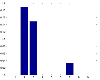
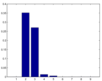
Figure 16: The values of the scales of the ARD kernel after training on the motion capture dataset using the exponentiated quadratic (fig: 16) and the Matérn (fig: 16) kernel to model the dynamics for the dynamical variational GP-LVM. The scales that have zero value “switch off” the corresponding dimension of the latent space. The latent space is, therefore, 3-D for 16 and 4-D for 16. Note that the scales were initialized with very similar values (e.g. a vector of ones with added random noise).

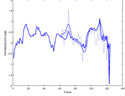
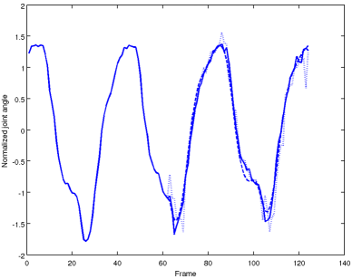
Figure 17: The prediction for two of the test angles for the body (fig: 17) and for the legs part (fig: 17). Continuous line is the original test data, dotted line is nearest neighbour in scaled space, dashed line is dynamical variational GP-LVM (using the exponentiated quadratic kernel for the body reconstruction and the Matérn for the legs).

As was explained in Section 5.3, all employed models encode the “walk” and “run” regime as two separate subspaces in the latent space. To illustrate this more clearly we sampled points from the learned latent space $\mathbf{{X}}$ of a trained dynamical variational GP-LVM model and generated the corresponding outputs, so as to investigate the kind of information that is encoded in each subspace of $\mathbf{{X}}$. Specifically, we considered the model that employed a Matérn $\frac{3}{2}$ covariance function to constrain the latent space and, based on the ARD weights of Figure 16, we projected the latent space on dimensions $(2,3)$ and $(2,4)$. Interacting with the model revealed that dimension $4$ separates the “walk” from the “run” regime. In particular, we first fixed dimension $4$ on a value belonging to the region encoding the walk, as can be seen in Figure 18, and then sampled multiple latent points by varying the other two dominant dimensions, namely $2$ and $3$, as can be seen in the top row of Figure 19. The corresponding outputs are shown in the second row of Figure 19. When dimension $4$ was fixed on a value belonging to the region encoding the run (Figure 18) the outputs obtained by varying dimensions $2$ and $3$ as before produced a smooth running motion, as can be seen in the third row of Figure 19. Finally, Figure 18 illustrates a motion which clearly is very different from the training set and was obtained by sampling a latent position far from the training data, as can be seen in Figure 18. This is indicative of a generative model’s ability of producing novel data.

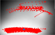
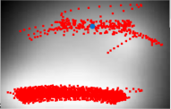
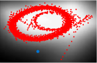
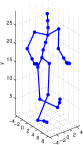
Figure 18: Plots 18 and 18 depict the projection of the latent space on dimensions $2$ and $4$, with the blue dot corresponding to the value on which these dimensions were fixed for the sampled latent points and red crosses represent latent points corresponding to training outputs. The intensity of the grayscale background represents the posterior uncertainty at each region (white corresponds to low predictive variance). Plot 18 depicts a latent space projection on dimensions $2$ and $3$, with the fixed latent positions corresponding to the generated output depicted in plot 18.

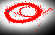
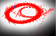
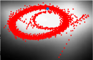
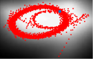
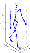
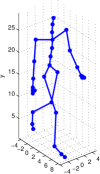
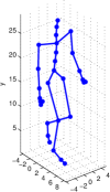
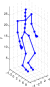
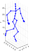
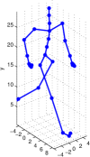
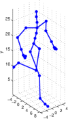
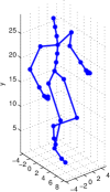
Figure 19: The first row depicts a projection of the latent space on dimensions $2$ and $3$ with the blue dot showing the value at which these dimensions were fixed for the sampled latent points. The corresponding outputs are depicted in the second row (for the walk regime) and third row (for the run regime).

References

- Bartholomew (1987) David J. Bartholomew. Latent Variable Models and Factor Analysis. Charles Griffin & Co. Ltd, London, 1987.
- Basilevsky (1994) Alexander Basilevsky. Statistical Factor Analysis and Related Methods. Wiley, New York, 1994.
- Belkin and Niyogi (2003) Mikhail Belkin and Partha Niyogi. Laplacian eigenmaps for dimensionality reduction and data representation. Neural Computation, 15(6):1373–1396, 2003. doi: 10.1162/089976603321780317.
- Bishop (1999) Christopher M. Bishop. Bayesian PCA. In Michael J. Kearns, Sara A. Solla, and David A. Cohn, editors, Advances in Neural Information Processing Systems, volume 11, pages 482–388, Cambridge, MA, 1999. MIT Press.
- Bishop (2006) Christopher M. Bishop. Pattern Recognition and Machine Learning. Springer-Verlag, 2006. ISBN 0387310738.
- Bishop and James (1993) Christopher M. Bishop and Gwilym D. James. Analysis of multiphase flows using dual-energy gamma densitometry and neural networks. Nuclear Instruments and Methods in Physics Research, A327:580–593, 1993. doi: 10.1016/0168-9002(93)90728-Z.
- Bishop et al. (1998) Christopher M. Bishop, Marcus Svensén, and Christopher K. I. Williams. GTM: the Generative Topographic Mapping. Neural Computation, 10(1):215–234, 1998. doi: 10.1162/089976698300017953.
- Csató (2002) Lehel Csató. Gaussian Processes — Iterative Sparse Approximations. PhD thesis, Aston University, 2002.
- Csató and Opper (2002) Lehel Csató and Manfred Opper. Sparse on-line Gaussian processes. Neural Computation, 14(3):641–668, 2002.
- Damianou and Lawrence (2013) Andreas Damianou and Neil D. Lawrence. Deep Gaussian processes. In Carlos Carvalho and Pradeep Ravikumar, editors, Proceedings of the Sixteenth International Workshop on Artificial Intelligence and Statistics, volume 31, AZ, USA, 2013. JMLR W&CP 31.
- Damianou et al. (2011) Andreas Damianou, Michalis K. Titsias, and Neil D. Lawrence. Variational Gaussian process dynamical systems. In Peter Bartlett, Fernando Peirrera, Chris Williams, and John Lafferty, editors, Advances in Neural Information Processing Systems, volume 24, Cambridge, MA, 2011. MIT Press.
- Damianou et al. (2012) Andreas Damianou, Carl Henrik Ek, Michalis K. Titsias, and Neil D. Lawrence. Manifold relevance determination. In John Langford and Joelle Pineau, editors, Proceedings of the International Conference in Machine Learning, volume 29, San Francisco, CA, 2012. Morgan Kauffman.
- Deisenroth et al. (2012) Marc Peter Deisenroth, Ryan Darby Turner, Marco F Huber, Uwe D Hanebeck, and Carl Edward Rasmussen. Robust filtering and smoothing with Gaussian processes. Automatic Control, IEEE Transactions on, 57(7):1865–1871, 2012.
- Ek et al. (2008) Carl Henrik Ek, Philip H.S. Torr, and Neil D. Lawrence. Gaussian process latent variable models for human pose estimation. In Andrei Popescu-Belis, Steve Renals, and Hervé Bourlard, editors, Machine Learning for Multimodal Interaction (MLMI 2007), volume 4892 of LNCS, pages 132–143, Brno, Czech Republic, 2008. Springer-Verlag. doi: 10.1007/978-3-540-78155-4˙12.
- Ferris et al. (2007) Brian D. Ferris, Dieter Fox, and Neil D. Lawrence. WiFi-SLAM using Gaussian process latent variable models. In Manuela M. Veloso, editor, Proceedings of the 20th International Joint Conference on Artificial Intelligence (IJCAI 2007), pages 2480–2485, 2007.
- Frigola et al. (2014) Roger Frigola, Fredrik Lindsten, Thomas B Schön, and Carl E Rasmussen. Identification of Gaussian process state-space models with particle stochastic approximation em. In 19th World Congress of the International Federation of Automatic Control (IFAC), Cape Town, South Africa, 2014.
- Fusi et al. (2013) Nicoló Fusi, Christoph Lippert, Karsten Borgwardt, Neil D. Lawrence, and Oliver Stegle. Detecting regulatory gene-environment interactions with unmeasured environmental factors. Bioinformatics, 2013. doi: 10.1093/bioinformatics/btt148.
- Gal et al. (2014) Yarin Gal, Mark van der Wilk, and Carl E. Rasmussen. Distributed variational inference in sparse Gaussian process regression and latent variable models. arXiv:1402.1389, 2014.
- Ghahramani (2007) Zoubin Ghahramani, editor. Proceedings of the International Conference in Machine Learning, volume 24, 2007. Omnipress. ISBN 1-59593-793-3.
- Girard et al. (2003) Agathe Girard, Carl Edward Rasmussen, Joaquin Quiñonero Candela, and Roderick Murray-Smith. Gaussian process priors with uncertain inputs—application to multiple-step ahead time series forecasting. In Sue Becker, Sebastian Thrun, and Klaus Obermayer, editors, Advances in Neural Information Processing Systems, volume 15, pages 529–536, Cambridge, MA, 2003. MIT Press.
- Goldberg et al. (1998) Paul W. Goldberg, Christopher K. I. Williams, and Christopher M. Bishop. Regression with input-dependent noise: A Gaussian process treatment. In Jordan et al. (1998), pages 493–499.
- Gordon et al. (1993) Neil J. Gordon, David J. Salmond, and Adrian F. M. Smith. Novel approach to nonlinear/non-Gaussian Bayesian state estimation. IEE Proceedings F Radar and Signal Processing, 140(2), 1993.
- Hyvärinen et al. (2001) Aapo Hyvärinen, Juha Karhunen, and Erkki Oja. Independent Component Analysis. John Wiley and Sons, 2001. ISBN 978-0-471-40540-5.
- Jordan et al. (1998) Michael I. Jordan, Michael J. Kearns, and Sara A. Solla, editors. Advances in Neural Information Processing Systems, volume 10, Cambridge, MA, 1998. MIT Press.
- Kersting et al. (2007) Kristian Kersting, Christian Plagemann, Patrick Pfaff, and Wolfram Burgard. Most likely heteroscedastic gaussian process regression. In Proceedings of the 24th international conference on Machine learning, ICML ’07, pages 393–400, New York, NY, USA, 2007. ACM. ISBN 978-1-59593-793-3. doi: 10.1145/1273496.1273546.
- King and Lawrence (2006) Nathaniel J. King and Neil D. Lawrence. Fast variational inference for Gaussian Process models through KL-correction. In ECML, Berlin, 2006, Lecture Notes in Computer Science, pages 270–281, Berlin, 2006. Springer-Verlag.
- Kingma and Welling (2013) Diederik P Kingma and Max Welling. Auto-encoding variational Bayes. arXiv preprint arXiv:1312.6114, 2013.
- Kingma et al. (2014) Diederik P. Kingma, Danilo Jimenez Rezende, Shakir Mohamed, and Max Welling. Semi-supervised learning with deep generative models. CoRR, abs/1406.5298, 2014.
- Ko and Fox (2009a) Jonathan Ko and Dieter Fox. GP-BayesFilters: Bayesian filtering using Gaussian process prediction and observation models. Auton. Robots, 27:75–90, July 2009a. ISSN 0929-5593. doi: 10.1007/s10514-009-9119-x. URL http://portal.acm.org/citation.cfm?id=1569248.1569255.
- Ko and Fox (2009b) Jonathan Ko and Dieter Fox. Learning GP-BayesFilters via Gaussian process latent variable models. In Robotics: Science and Systems, 2009b.
- Ko and Fox (2009c) Jonathan Ko and Dieter Fox. GP-BayesFilters: Bayesian filtering using Gaussian process prediction and observation models. Autonomous Robots, 27:75–90, July 2009c. ISSN 0929-5593. doi: 10.1007/s10514-009-9119-x.
- Ko and Fox (2011) Jonathan Ko and Dieter Fox. Learning GP-Bayesfilters via Gaussian process latent variable models. Autonomous Robots, 30:3–23, 2011. ISSN 0929-5593. URL http://dx.doi.org/10.1007/s10514-010-9213-0. 10.1007/s10514-010-9213-0.
- Lawrence (2004) Neil D. Lawrence. Gaussian process models for visualisation of high dimensional data. In Sebastian Thrun, Lawrence Saul, and Bernhard Schölkopf, editors, Advances in Neural Information Processing Systems, volume 16, pages 329–336, Cambridge, MA, 2004. MIT Press.
- Lawrence (2005) Neil D. Lawrence. Probabilistic non-linear principal component analysis with Gaussian process latent variable models. Journal of Machine Learning Research, 6:1783–1816, 11 2005.
- Lawrence (2006) Neil D. Lawrence. The Gaussian process latent variable model. Technical Report CS-06-03, The University of Sheffield, Department of Computer Science, 2006.
- Lawrence (2007) Neil D. Lawrence. Learning for larger datasets with the Gaussian process latent variable model. In Marina Meila and Xiaotong Shen, editors, Proceedings of the Eleventh International Workshop on Artificial Intelligence and Statistics, pages 243–250, San Juan, Puerto Rico, 21-24 March 2007. Omnipress.
- Lawrence (2012) Neil D. Lawrence. A unifying probabilistic perspective for spectral dimensionality reduction: Insights and new models. Journal of Machine Learning Research, 13, 2012. URL http://jmlr.csail.mit.edu/papers/v13/lawrence12a.html.
- Lawrence and Moore (2007) Neil D. Lawrence and Andrew J. Moore. Hierarchical Gaussian process latent variable models. In Ghahramani (2007), pages 481–488. ISBN 1-59593-793-3.
- Lázaro-Gredilla (2012) Miguel Lázaro-Gredilla. Bayesian warped Gaussian processes. In Peter L. Bartlett, Fernando C. N. Pereira, Christopher J. C. Burges, Léon Bottou, and Kilian Q. Weinberger, editors, Advances in Neural Information Processing Systems, volume 25, Cambridge, MA, 2012.
- Lázaro-Gredilla and Titsias (2011) Miguel Lázaro-Gredilla and Michalis K. Titsias. Variational heteroscedastic gaussian process regression. In In 28th International Conference on Machine Learning (ICML-11, pages 841–848. ACM, 2011.
- Leen et al. (2001) Todd K. Leen, Thomas G. Dietterich, and Volker Tresp, editors. Advances in Neural Information Processing Systems, volume 13, Cambridge, MA, 2001. MIT Press.
- Lu and Tang (2014) Chaochao Lu and Xiaoou Tang. Surpassing human-level face verification performance on LFW with GaussianFace. CoRR, abs/1404.3840, 2014.
- MacKay (1998) D. J. C. MacKay. Introduction to Gaussian processes. In C. M. Bishop, editor, Neural Networks and Machine Learning, NATO ASI Series, pages 133–166. Kluwer Academic Press, 1998.
- MacKay (1995) David J. C. MacKay. Bayesian neural networks and density networks. Nuclear Instruments and Methods in Physics Research, A, 354(1):73–80, 1995. doi: 10.1016/0168-9002(94)00931-7.
- Mardia et al. (1979) Kantilal V. Mardia, John T. Kent, and John M. Bibby. Multivariate analysis. Academic Press, London, 1979. ISBN 0-12-471252-5.
- McHutchon and Rasmussen (2011) Andrew McHutchon and Carl Edward Rasmussen. Gaussian process training with input noise. In NIPS’11, pages 1341–1349, 2011.
- Minka (2001) Thomas P. Minka. Automatic choice of dimensionality for PCA. In Leen et al. (2001), pages 598–604.
- Oakley and O’Hagan (2002) Jeremey Oakley and Anthony O’Hagan. Bayesian inference for the uncertainty distribution of computer model outputs. Biometrika, 89(4):769–784, 2002.
- Opper and Archambeau (2009) Manfred Opper and Cédric Archambeau. The variational Gaussian approximation revisited. Neural Computation, 21(3):786–792, 2009.
- Quiñonero Candela and Rasmussen (2005) Joaquin Quiñonero Candela and Carl Edward Rasmussen. A unifying view of sparse approximate Gaussian process regression. Journal of Machine Learning Research, 6:1939–1959, 2005.
- Quiñonero-Candela et al. (2003) Joaquin Quiñonero-Candela, Agathe Girard, Jan Larsen, and Carl Edward Rasmussen. Propagation of uncertainty in bayesian kernel models-application to multiple-step ahead forecasting. In Acoustics, Speech, and Signal Processing, 2003. Proceedings.(ICASSP’03). 2003 IEEE International Conference on, volume 2, pages II–701. IEEE, 2003.
- Rasmussen and Williams (2006) Carl Edward Rasmussen and Christopher K. I. Williams. Gaussian Processes for Machine Learning. MIT Press, Cambridge, MA, 2006. ISBN 0-262-18253-X.
- Rosenberg et al. (2005) C. Rosenberg, M. Hebert, and H. Schneiderman. Semi-supervised self-training of object detection models. In Application of Computer Vision, 2005. WACV/MOTIONS ’05 Volume 1. Seventh IEEE Workshops on, volume 1, pages 29–36, Jan 2005. doi: 10.1109/ACVMOT.2005.107.
- Roweis (1998) Sam T. Roweis. EM algorithms for PCA and SPCA. In Jordan et al. (1998), pages 626–632.
- Roweis and Saul (2000) Sam T. Roweis and Lawrence K. Saul. Nonlinear dimensionality reduction by locally linear embedding. Science, 290(5500):2323–2326, 2000. doi: 10.1126/science.290.5500.2323.
- Sammon (1969) John W. Sammon. A nonlinear mapping for data structure analysis. IEEE Transactions on Computers, C-18(5):401–409, 1969. doi: 10.1109/T-C.1969.222678.
- Särkkä (2013) Simo Särkkä. Bayesian Filtering and Smoothing. Cambridge University Press, 2013. ISBN 9781107619289.
- Schölkopf et al. (1998) Bernhard Schölkopf, Alexander Smola, and Klaus-Robert Müller. Nonlinear component analysis as a kernel eigenvalue problem. Neural Computation, 10:1299–1319, 1998. doi: 10.1162/089976698300017467.
- Seeger et al. (2003) Matthias Seeger, Christopher K. I. Williams, and Neil D. Lawrence. Fast forward selection to speed up sparse Gaussian process regression. In Christopher M. Bishop and Brendan J. Frey, editors, Proceedings of the Ninth International Workshop on Artificial Intelligence and Statistics, Key West, FL, 3–6 Jan 2003.
- Smola and Bartlett (2001) Alexander J. Smola and Peter L. Bartlett. Sparse greedy Gaussian process regression. In Leen et al. (2001), pages 619–625.
- Snelson and Ghahramani (2006) Edward Snelson and Zoubin Ghahramani. Sparse Gaussian processes using pseudo-inputs. In Weiss et al. (2006).
- Snelson et al. (2004) Edward Snelson, Carl Edward Rasmussen, and Zoubin Ghahramani. Warped Gaussian processes. Advances in Neural Information Processing Systems, 16:337–344, 2004.
- Taylor et al. (2007) Graham W. Taylor, Geoffrey E. Hinton, and Sam Roweis. Modeling human motion using binary latent variables. In Bernhard Schölkopf, John C. Platt, and Thomas Hofmann, editors, Advances in Neural Information Processing Systems, volume 19, Cambridge, MA, 2007. MIT Press.
- Tenenbaum et al. (2000) Joshua B. Tenenbaum, Virginia de Silva, and John C. Langford. A global geometric framework for nonlinear dimensionality reduction. Science, 290(5500):2319–2323, 2000. doi: 10.1126/science.290.5500.2319.
- Tipping and Bishop (1999) Michael E. Tipping and Christopher M. Bishop. Probabilistic principal component analysis. Journal of the Royal Statistical Society, B, 6(3):611–622, 1999. doi: doi:10.1111/1467-9868.00196.
- Titsias (2009a) Michalis Titsias. Variational learning of inducing variables in sparse Gaussian processes. JMLR W&CP, 5:567–574, 2009a.
- Titsias and Lázaro-Gredilla (2013) Michalis Titsias and Miguel Lázaro-Gredilla. Variational inference for mahalanobis distance metrics in Gaussian process regression. In C.J.C. Burges, L. Bottou, M. Welling, Z. Ghahramani, and K.Q. Weinberger, editors, Advances in Neural Information Processing Systems 26, pages 279–287. Curran Associates, Inc., 2013.
- Titsias (2009b) Michalis K. Titsias. Variational learning of inducing variables in sparse Gaussian processes. In David van Dyk and Max Welling, editors, Proceedings of the Twelfth International Workshop on Artificial Intelligence and Statistics, volume 5, pages 567–574, Clearwater Beach, FL, 16-18 April 2009b. JMLR W&CP 5.
- Urtasun and Darrell (2007) Raquel Urtasun and Trevor Darrell. Discriminative Gaussian process latent variable model for classification. In Ghahramani (2007). ISBN 1-59593-793-3.
- Urtasun et al. (2006) Raquel Urtasun, David J. Fleet, and Pascal Fua. 3D people tracking with Gaussian process dynamical models. In Proceedings of the IEEE Computer Society Conference on Computer Vision and Pattern Recognition, pages 238–245, New York, U.S.A., 17–22 Jun. 2006. IEEE Computer Society Press. doi: 10.1109/CVPR.2006.15.
- van der Maaten and Hinton (2008) Larens J. P. van der Maaten and Geoffrey E. Hinton. Visualizing data using t-SNE. Journal of Machine Learning Research, 9:2579–2605, 2008.
- Wang et al. (2006) Jack M. Wang, David J. Fleet, and Aaron Hertzmann. Gaussian process dynamical models. In Weiss et al. (2006).
- Wang et al. (2008) Jack M. Wang, David J. Fleet, and Aaron Hertzmann. Gaussian process dynamical models for human motion. IEEE Transactions on Pattern Analysis and Machine Intelligence, 30(2):283–298, 2008. ISSN 0162-8828. doi: 10.1109/TPAMI.2007.1167.
- Weiss et al. (2006) Yair Weiss, Bernhard Schölkopf, and John C. Platt, editors. Advances in Neural Information Processing Systems, volume 18, Cambridge, MA, 2006. MIT Press.