Preliminary Evaluation of the Kepler Input Catalog Extinction Model Using Stellar Temperatures

Abstract

The Kepler Input Catalog (KIC) provides reddening estimates for its stars, based on the assumption of a simple exponential dusty screen. This project focuses on evaluating and improving these reddening estimates for the KIC’s giant stars, for which extinction is a much more significant concern than for the nearby dwarf stars. We aim to improve the calibration (and thus consistency) amongst various photometric and spectroscopic temperatures of stars in the Kepler field by removing systematics due to incorrect extinction assumptions. The revised extinction estimates may then be used to derive improved stellar and planetary properties. We plan to eventually use the large number of KIC stars as probes into the structure and properties of the Galactic ISM.

1 Introduction

The dusty interstellar medium (ISM) of the Milky Way (MW) permeates the entire galaxy, with non-zero reddening observed even at the Galactic poles. Even though the effects of extinction at infrared (IR) wavelengths are smaller than those at optical wavelengths, both optical and near-IR images of the MW demonstrate that interstellar dust is strongly concentrated in the midplane but not exclusively confined there. And the Kepler field, lying $5^{\circ}-20^{\circ}$ off the midplane, is hardly free of its effects. One of the major problems with unaccounted-for extinction is that it changes properties inferred from photometry (e.g., luminosity, distance, temperature) in a systematic way — stars always look cooler and fainter, never the other way around.

Of course, much effort has been made to address this issue, leading to a large number of extinction maps and models derived using a variety of methods and ISM tracers. To name just a few examples, Drimmel et al. (2003) and Drimmel & Spergel (2001) have built an analytic model of the MW’s ISM, complete with a smooth disk and superimposed dusty spiral arms. The commonly adopted all-sky reddening maps by Schlegel et al. (1998) use primarily the dust emission at 100 $\mu$m to trace extinction, along with some assumptions about the dust homogeneity that make the maps tricky to apply within 20^∘ or so of the midplane. Marshall et al. (2006) compared NIR color-magnitude diagrams to those predicted by the Besançon MW stellar populations model and published extinction maps spanning the MW’s midplane. Very recently, Gonzalez et al. (2012) published maps of the Galactic bulge, using red clump stars from the VVV to trace extinction on arcmin scales.

In comparison, the Kepler Input Catalog (KIC) assumed the extinction model of a smooth, vertically-exponential dust disk, with a scaleheight $H$ of 150 pc and an extinction density $\kappa_{0}$ normalized to 1 mag of $V$-band extinction per kpc at $b=0^{\circ}$:

$$E(B-V)_{\rm KIC}=0.367\kappa_{0}\int_{0}^{d}e^{-\frac{s}{H}\sin{b}}{\rm d}s,$$ (1)

(adapted from Brown et al., 2011). Thus the reddening can be parameterized as a function of distance $d$ and latitude $b$ alone, with typical values for the KIC stars of $E(B-V)\sim 0.05-0.18$ mag. However, the KIC stellar parameters were derived simultaneously along with the reddening, meaning that the final $E(B-V)$ values are implicitly tied to all of the parameters, including the effective temperature ($T_{\rm eff}$) and the metallicity. These correlations mean that the catalog reddening values have strong implications for other properties of interest further down the pipeline, such as planetary radii or the stellar distances derived using the KIC parameters in other methods, which are important for any Galactic structure work or study of metallicity or age gradients (to name but a few possibilities).

2 Comparison of Photometric and Spectroscopic Temperatures

In the top left panel of Figure 1, we show the comparison between two photometric temperature methods: the original KIC $T_{\rm eff}$ values and those derived from SDSS griz colors by Pinsonneault et al. (2012). An offset of $\sim$100–200 K demonstrates that adopting the KIC reddening values, along with internally consistent color-$T_{\rm eff}$ relations, would give rise to systematically hotter temperatures. The bottom panel of Figure 1 shows that the griz temperatures (corrected for giant stars) are far more consistent with those derived with the InfraRed Flux Method (IRFM; Casagrande et al., 2010), which arguably represent a more fundamental measurement of effective temperature as it is defined.

Figure 1: Left: Comparison between the SDSS griz $T_{\rm eff}$ values and (top) the KIC $T_{\rm eff}$ and (bottom) IRFM $T_{\rm eff}$ for giant stars. (Figure 18 of ref Pinsonneault et al., 2013). Right: Difference between the SDSS griz $T_{\rm eff}$ values and those from APOGEE/ASPCAP, as a function of SDSS $T_{\rm eff}$, for the $\sim$2000 giants in the APOKASC sample.

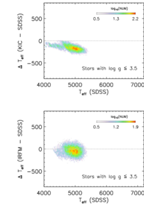
At least two studies have targeted Kepler stars for spectroscopic followup and evaluation of the KIC stellar parameters. Thygesen et al. (2012) and Molenda-Żakowicz et al. (2013) observed a total of $\sim$200 stars, and both found an offset of up to a couple hundred K (which was strongly $T_{\rm eff}$-dependent in Thygesen et al., 2012).

A much larger spectroscopic comparison sample is provided by the APOKASC program, a collaboration between APOGEE, a high-resolution, $H$-band spectroscopic survey of MW red giant stars (Majewski, 2012), and KASC, the core working group of Kepler asteroseismic science. The APOKASC team is combining asteroseismic and spectroscopic measurements and their respective derived parameters for $\sim$10⁴ stars (see Section 8.3 of Zasowski et al., 2013). The APOKASC catalog at the time of this proceeding contains $\sim$2000 giant stars, an increase of nearly an order of magnitude over the previous sample. Figure 1 also shows the comparison between the photometric griz $T_{\rm eff}$ and the spectroscopic APOGEE $T_{\rm eff}$, where the latter have been “corrected” to a temperature scale calibrated to a number of well-studied star clusters. Despite this correction, a strongly temperature-dependent offset is clearly present, in addition to a $\pm$100 K scatter. Possible reasons for the persistent discrepancy include systematic offsets in the APOGEE pipeline and/or potential errors in the theoretical corrections applied to the dwarf-derived griz-$T_{\rm eff}$ relations to make them suitable for giants.

2.1 Impact of Extinction?

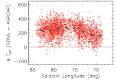
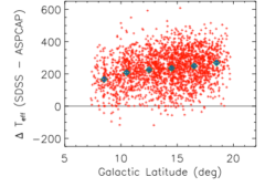
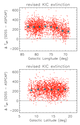
Figure 2 shows the difference between the griz temperatures (which assume a reddening value) and the APOGEE temperatures (which do not), as functions of Galactic longitude (left) and latitude (right). There is no monotonic trend with longitude, though there are hints of coherent structure, but there is a systematic trend with latitude. As any observed $T_{\rm eff}$ offsets should be independent of spatial position, the behavior seen here suggests a problem with the extinction model, which is smooth in longitude but dependent on latitude. In order to test the form and scale of the KIC extinction model, we require a large number of KIC stellar extinction estimates that do not depend on any global Galactic model (which would unavoidably include its own assumptions about the underlying dust structure).

Figure 2: Difference in griz $T_{\rm eff}$ and APOGEE/ASPCAP $T_{\rm eff}$ as a function of (left) Galactic longitude and (right) Galactic latitude, assuming the original KIC reddening.

3 Revision of the KIC Extinctions

3.1 RJCE Extinctions

For independent extinction estimates, we turn to the Rayleigh-Jeans Color Excess method (RJCE; Majewski et al., 2011), which provides stellar foreground extinction estimates based on the star’s near- and mid-IR photometry. Like other color excess methods, the basis of RJCE is the assumption that all stars in a given sample have a common intrinsic color, such that any observed excess in that color may be attributed to line-of-sight reddening. Where RJCE improves upon earlier color excess approaches is in the combination of NIR+MIR photometry, which sample the Rayleigh-Jeans (RJ) tail of a star’s spectral energy distribution (SED). The slope of the RJ tail is almost entirely independent of stellar temperature or metallicity, which means that colors comprising filters measuring this part of the SED are truly homogeneous across a very large fraction of the MW’s stellar populations. In contrast, color excess methods relying on more temperature-dependent optical or NIR-only colors must know a priori, or assume, the spectral type of the stars under consideration. See Majewski et al. (2011) for an expanded description and example applications of the RJCE approach.

Most relevant for the current analysis is that the RJCE extinction values are free from assumptions about the spatial distribution of the MW’s dust content and thus provide a good comparison to the KIC values, which are strongly dependent on the KIC’s assumed dust disk model. Also relevant are some caveats on RJCE’s applicability. Due to [Fe/H]-dependent spectral features, very metal-poor stars (${\rm[Fe/H]}<-1.5$) appear to have intrinsic colors deviating from those assumed in RJCE, such that their extinction values are systematically overestimated. Fortunately, such stars are relatively rare in the Kepler field. The uncertainties in the RJCE extinction values arise from the photometric uncertainties as well as uncertainty in the adopted extinction law; typical values for the KIC sample are $\sigma(A[K_{s}])<0.05$ mag.

3.2 Extinction Map Comparison

For this initial assessment of the KIC extinction, we used stars meeting the following criteria: $A(K_{s})_{\rm RJCE}\geq 0$, $\sigma(A[K_{s}])_{\rm RJCE}\leq 0.05$, 2MASS nearest neighbor distance (prox) of $\geq$10^′′, $4000\leq(T_{\rm eff})_{\rm KIC}\leq 5000$ K, and $(\log{g})_{\rm KIC}\leq 3.7$. These requirements produced a sample of $\sim$13 500 red giant stars with well-measured RJCE extinction values.

This sample includes stars as faint as $H\sim 15$, while the spectroscopic APOKASC sample is limited to stars with $H\leq 11$. Because we want to ensure that any corrections calculated are applicable to the stars being corrected, we performed the analysis below both with and without an $H\leq 11$ limit on the sample. We found that this limit actually had little-to-no impact on the outcome, which is a result of the fact that stars in our sample with $H\leq 11$ have a very similar extinction distribution (in RJCE and the KIC) as those with $11<H<15$. Since the fainter giants comprise more distant stars, as well as intrinsically fainter ones, this result may be somewhat surprising, given the assumption of a strongly distance-dependent extinction distribution. What this suggests is that a foreground extinction screen model may be appropriate for this particular sample (certainly not generally applicable to MW stellar populations!), which provides further justification for the approach adopted below (in which we do not apply the $H\leq 11$ limit). Of course, the KIC extinction values are distance dependent, and there is a slightly larger discrepancy between the $E(B-V)$ distributions of the $H\leq 11$ and $11<H<15$ subsamples than between the RJCE reddening distributions of the same subsamples, but the discrepancy is still not large enough to significantly affect the outcome below.

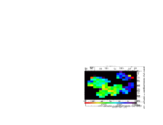
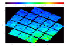
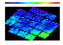
We created two extinction maps spanning the entire Kepler field, taking as the value of each 0.4^∘$\times$0.2^∘ pixel the median KIC $E(B-V)$ or RJCE $A(K_{s})$ extinction of the stars in that pixel (Figure 3, where we have converted the KIC $E(B-V)$ to $A(K_{s})$ for comparison purposes). This pixel size was chosen to ensure $\geq$10 stars per bin, and the asymmetry reflects the fact that in both maps, the variations in $b$ have a shorter scale than those in $l$. We chose to parameterize this first “correction” with a zero-point offset, an extinction-dependent scale factor, and a $b$-dependent scale factor.

Figure 3: Left: Median map of KIC $A(K_{s})$ values, assuming $A(K_{s})=0.388\times E(B-V)$. Right: Median map of RJCE $A(K_{s})$ values.

3.3 Results

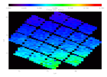
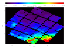
The fitting of the KIC map to the RJCE one yields: $E(B-V)=E(B-V)_{\rm KIC}\times(1.29-1.75\,\sin{b})+0.02$. The median extinction map using these fitted KIC reddening values is shown in the left panel of Figure 4. The impact of this correction scaling is to reduce the effective scaleheight of the KIC model’s dust layer, whose original value was even noted in Brown et al. (2011) to be larger than the literature suggested, and to bring the reddening values more in line with those calculated from the independent RJCE method (i.e., compare Figure 3 [right] with Figure 4 [left]). As a further sanity check, we compare the revised KIC map with the Schlegel et al. (1998) dust map (Figure 4, right), and we see much better agreement with the revised map than with the original KIC one, in terms of latitude dependence.

Figure 4: Left: Median map of revised KIC $A(K_{s})$ values. Right: Median map of Schlegel et al. (1998) $A(K_{s})$ values.

In the left column of Figure 5, we show that the revised map clearly mitigates the spatial dependencies of the offsets between the photometric griz temperatures and the spectroscopic APOGEE ones. In the top panel, the longitude structure is reduced (but not eliminated, suggesting further improvement can be made; §4), and in the bottom panel, the latitude dependence has disappeared entirely. Note that there is still a $\sim$200 K offset — the revised reddening map has not solved the entire problem, but it does remove that particular systematic contribution to the behavior.

Figure 5: Left: Difference in $T_{\rm eff}$ from SDSS colors and from APOGEE/ASPCAP as functions of (top) Galactic longitude and (bottom) Galactic latitude, using the revised KIC reddening. Compare to Figure 2. Right: Difference in $T_{\rm eff}$ calculated with the IRFM method (Casagrande et al., 2010) and with SDSS griz colors, assuming (top) the original KIC reddening and (bottom) the revised KIC reddening.

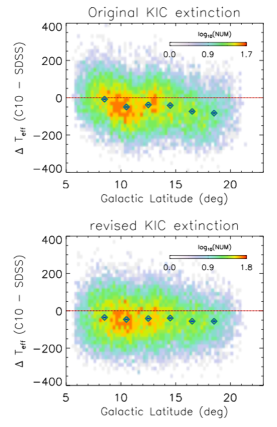
The reddening revisions even appear to reduce some systematics in the comparison of photometric temperatures. The right-hand column of Figure 5 shows the difference between the IRFM and the griz $T_{\rm eff}$ values as a function of $b$, using the original KIC $E(B-V)$ (top) and the revised $E(B-V)$ (bottom). Both of these methods use extinction estimates but to different degrees. Thus, an offset trend with $b$ is visible (though weaker than in the comparison to spectroscopic $T_{\rm eff}$) but disappears with the revised reddening, most noticeably at higher $b$.

4 Future Improvements

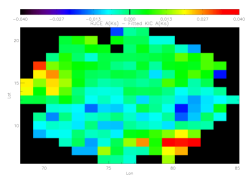
A number of improvements to these preliminary results are actively in progress, including incorporation of substructure parameterization into the KIC model fitting. The $\Delta E(B-V)$ residuals observed between the RJCE and the revised KIC maps are not dominated by random noise (Figure 6). The presence of coherent clumps and gradients implies real structure in the ISM not accounted for by the KIC’s exponential disk model. For example, the residual map shows a clump at $(l,b)\sim(70.5^{\circ},14^{\circ})$, clearly visible in the RJCE and Schlegel maps but not in the smooth KIC one. This cloud corresponds to roughly 0.1 mag of $E(B-V)$ reddening above the background reproduced in the KIC map. Thus, identifying and parameterizing these irregular variations will have a significant impact on many stars.

t]

Figure 6: Difference between the revised KIC extinction map and the RJCE map, in $A(K_{s})$.