Smart Sampling for Lightweight Verification
of Markov Decision Processes

Abstract

Markov decision processes (MDP) are useful to model optimisation problems in concurrent systems. To verify MDPs with efficient Monte Carlo techniques requires that their nondeterminism be resolved by a scheduler. Recent work has introduced the elements of lightweight techniques to sample directly from scheduler space, but finding optimal schedulers by simple sampling may be inefficient. Here we describe “smart” sampling algorithms that can make substantial improvements in performance.

I Introduction

Markov decision processes describe systems that interleave nondeterministic actions and probabilistic transitions. This model has proved useful in many real optimisation problems [27, 28, 29] and may be used to represent concurrent probabilistic programs (see, e.g., [3, 1]). Such models comprise probabilistic subsystems whose transitions depend on the states of the other subsystems, while the order in which concurrently enabled transitions execute is nondeterministic. This order may radically affect the behaviour of a system and it is thus useful to calculate the upper and lower bounds of quantitative aspects of performance.

As an example, consider the network of computational nodes depicted in Fig. 2 (relating to the case study in Section VI-D). Given that one of the nodes is infected by a virus, we would like to calculate the probability that a target node becomes infected. If we know the probability that the virus will pass from one node to the next, we could model the system as a discrete time Markov chain and analyse it to find the probability that any particular node will become infected. Such a model ignores the possibility that the virus might actually choose which node to infect, e.g., to maximise its probability of passing through the barrier layer. Under such circumstances some nodes might be infected with near certainty or with only very low probability, but this would not be adequately captured by the Markov chain. By modelling the virus’s choice of node as a nondeterministic transition in an MDP, the maximum and minimum probabilities of infection can be considered.

Figure 1: Model of network virus infection.

Figure 2: Fragment of a Markov decision process.

Fig. 2 shows a typical fragment of an MDP. Its execution semantics are as follows. In a given state ($s_{0}$), an action ($a_{1},a_{2},\dots$) is chosen nondeterministically to select a distribution of probabilistic transitions ($p_{1},p_{2},\dots$ or $p_{3},p_{4}$, etc.). A probabilistic choice is then made to select the next state ($s_{1},s_{2},s_{3},s_{4},\dots$). In this work we use the term scheduler to refer to a particular way the nondeterminism in an MDP is resolved.

Classic analysis of MDPs is concerned with finding the expected maximum or minimum reward for an execution of the system, given individual rewards assigned to each of the actions [2, 25]. Rewards may also be assigned to states or transitions between states [16]. In this work we focus on MDPs in the context of model checking concurrent probabilistic systems, to find schedulers that maximise or minimise the probability of a property. Model checking is an automatic technique to verify that a system satisfies a property specified in temporal logic [7]. Probabilistic model checking quantifies the probability that a probabilistic system will satisfy a property [9]. Numerical model checking algorithms to solve purely probabilistic systems are costly in time and space. Finding extremal probabilities in MDPs is generally more so, but is nevertheless a polynomial function of the explicit description of the MDP [3].

Statistical model checking (SMC) describes a collection of Monte Carlo sampling techniques that make probabilistic model checking more tractable by returning approximative results with statistical confidence [31]. Recent approaches to apply SMC to MDPs [4, 21, 11, 10, 22] are memory-intensive and do not fully address the nondeterministic model checking problem. Classic sampling approaches for MDPs, such as the Kearns algorithm [14], address a related but different problem.

This work extends [22]. In [22] the authors provide sampling techniques that can form the basis of memory-efficient (“lightweight”) verification of MDPs. The principal contributions of [22] are (i) specifying the infinite behaviour of history-dependent or memoryless schedulers using $\mathcal{O}(1)$ memory, (ii) sampling directly and uniformly from scheduler space, and (iii) quantifying the statistical confidence of multiple estimates or multiple hypothesis tests. As in the case of standard SMC, sampling makes the verification problem independent of the size of the space of samples, with a convergence to the correct result almost surely guaranteed with an infinite number of samples. The use of lightweight techniques opens up the possibility to efficiently distribute the problem on high performance massively parallel architectures, such as general purpose computing on graphics processing units (GPGPU).

Sampling schedulers makes a significant advance over mere enumeration. For example, suppose half of all schedulers for a given MDP and property are ‘near optimal’, i.e., have a probability of satisfying the property that is deemed adequately close to the true optimum. If all such near optimal schedulers lie in the second half of the enumeration, it will be necessary to enumerate half of all schedulers before finding one that is near optimal. In contrast, one would expect to see a near optimal scheduler after just two random selections, i.e., the expectation with two samples is one. This phenomenon is not limited to the case when schedulers are pathologically distributed with respect to the enumeration. Since the total number of schedulers increases exponentially with path length (the number of history-dependent schedulers increases doubly exponentially with states and path length), the total number of schedulers is usually very large. Hence, even when near optimal schedulers are more uniformly distributed with respect to the enumeration, it is typically not tractable to use enumeration to find one. Note that sampling also works with non-denumerable spaces. The cost of finding a near optimal scheduler with sampling is simply proportional to the relative mass of near optimal schedulers in scheduler space. Our experiments with standard case studies suggest that this cost is typically reasonable.

It was demonstrated in [22] that simple undirected sampling may be adequate for some case studies. In this work we present “smart sampling” algorithms that make significantly better use of a simulation budget. For a given number of candidate schedulers, smart sampling can reduce the simulation cost of extremal probability estimation by more than $N/\lceil 2+\log_{2}N\rceil$, where $N$ is the minimum number of simulations necessary to achieve the required statistical confidence, as given by (1). The basic notions of smart sampling were hinted at in [22]. Simply put, a small part of the budget is used to perform an initial assessment of the problem and to generate an optimal candidate set of schedulers. The remaining budget is used to test and refine the candidate set: sub-optimal schedulers are removed and their budget is re-allocated to good ones. Here we give a full exposition of smart sampling and explain its limitations. We have implemented the algorithms in our statistical model checking platform, Plasma, and demonstrate their successful application to a number of case studies from the literature. We include some examples that are intractable to numerical techniques and compare the performance of our techniques with an alternative sampling approach [11]. We also give an example where smart sampling is less effective, but show that the results may nevertheless be useful in bounding the range of extremal probabilities.

Structure of the Paper

In Section II we introduce some basic concepts and notation necessary for the sequel. In Section III we briefly survey closely related work. In Sections IV we recall the basis of our lightweight verification techniques. In Section V we describe the notion of smart sampling and present our smart estimation and smart hypothesis testing algorithms. In Section VI we give the results of experiments with a number of case studies from the literature. In Section VII we discuss the limitations of smart sampling and in Section VIII we summarise the challenges and prospects for our approach.

II Preliminaries

Given an MDP with set of actions $A$, having a set of states $S$ that induces a set of sequences of states $\Omega=S^{+}$, a history-dependent (general) scheduler is a function $\mathfrak{S}:\Omega\rightarrow A$. A memoryless scheduler is a function $\mathfrak{M}:S\rightarrow A$. Intuitively, at each state in the course of an execution, a general scheduler ($\mathfrak{S}$) chooses an action based on the sequence of previous states and a memoryless scheduler ($\mathfrak{M}$) chooses an action based only on the current state. History-dependent schedulers therefore include memoryless schedulers.

Figure 3: MDP with different optima for general and memoryless schedulers.

Fig. 3 illustrates a simple MDP for which memoryless and history-dependent schedulers give different optima for the bounded temporal logic property $\mathbf{X}(\psi\wedge\mathbf{XG}^{t}\neg\psi)$ when $p_{1}\neq p_{2}$ and $t>0$. The property makes use of the temporal operators next ($\mathbf{X}$) and globally ($\mathbf{G}$). Intuitively, the property states that on the next step $\psi$ will be true and, on the step after that, $\neg\psi$ will be remain true for $t+1$ time steps. The property is satisfied by the sequence of states $s_{0}s_{1}s_{0}s_{0}\cdots$. If $p_{1}>p_{2}$, the maximum probability for $s_{0}s_{1}$ is achieved with action $a_{2}$, while the maximum probability for $s_{0}s_{0}$ is achieved with action $a_{1}$. Given that both transitions start in the same state, a memoryless scheduler will not achieve the maximum probability achievable with a history-dependent scheduler.

Statistical Model Checking with Plasma

The algorithms we present here are implemented in our SMC platform Plasma (Platform for Learning and Advanced Statistical Model checking Algorithms [5]). Plasma is modular, allowing new modelling languages, logics and algorithms to be plugged-in and take advantage of its graphical user interface, its integrated development environment and its ability to correctly divide simulations on parallel computational architectures. We introduce here the basic features of SMC with Plasma that are relevant to what follows.

SMC algorithms work by constructing an automaton to accept only traces that satisfy a specified property. The state space of the system is not constructed explicitly – states are generated on the fly during simulation – hence SMC is efficient for large, possibly infinite state, systems. Moreover, since the simulations are required to be statistically independent, SMC may be efficiently divided on parallel computing architectures. The automaton may then be used to estimate the probability of the property or to decide an hypothesis about the probability. Typically, the probability $p$ of property $\varphi$ is estimated by the proportion of traces that individually satisfy it, i.e., $p\approx\frac{1}{N}\sum_{i=1}^{N}\mathbf{1}(\omega_{i}\models\varphi)$, where $\omega_{1},\dots,\omega_{N}$ are $N$ independently generated simulation traces and $\mathbf{1}(\cdot)$ is an indicator function that corresponds to the output of the automaton: it returns $1$ if the trace is accepted and $0$ if it is not. As a statistical process, the results of SMC are given with probabilistic confidence.

In the case of estimation, Plasma calculates a priori the required number of simulations according to a Chernoff bound [24] that allows the user to specify an error $\varepsilon$ and a probability $\delta$ that the estimate $\hat{p}$ will not lie outside the true value $\pm\varepsilon$. Given that a system has true probability $p$ of satisfying a property, the Chernoff bound ensures $\mathrm{P}(\mid\hat{p}-p\mid\geq\varepsilon)\leq\delta$. Parameter $\delta$ is related to the number of simulations $N$ by $\delta=2e^{-2N\varepsilon^{2}}$ [24], giving

$$N=\left\lceil(\ln 2-\ln\delta)/(2\varepsilon^{2})\right\rceil.$$ (1)

In the case of hypothesis testing, Plasma adopts the sequential probability ratio test (SPRT) of Wald [26] to test hypotheses of the form $\mathrm{P}(\omega\models\varphi)\bowtie\theta$, where $\bowtie\in\{\leq,\geq\}$ and $\theta$ is a user-specified probability threshold. The number of simulations required to decide the test is typically fewer than (1) but is dependent on how close $\theta$ is to the true probability. The number is therefore not known in advance. To evaluate $\mathrm{P}(\omega\models\varphi)\bowtie\theta$, the SPRT constructs hypotheses $H{}_{0}:\mathrm{P}(\omega\models\varphi)\geq p_{0}$ and $H{}_{1}:\mathrm{P}(\omega\models\varphi)\leq p_{1}$, where $p_{0}=\theta+\varepsilon$ and $p_{1}=\theta-\varepsilon$ for some user-defined interval specified by $\varepsilon$ [26]. The SPRT also requires parameters $\alpha$ and $\beta$ to specify, respectively, the maximum acceptable probabilities of incorrectly rejecting a true $H_{0}$ and incorrectly accepting a false $H_{0}$. To choose between $H_{0}$ and $H_{1}$, the SPRT defines the probability ratio

$$\mathit{ratio}=\prod_{i=1}^{n}\frac{(p^{1})^{\mathbf{1}(\omega_{i}\models\varphi)}(1-p^{1})^{\mathbf{1}(\omega_{i}\not\models\varphi)}}{(p^{0})^{\mathbf{1}(\omega_{i}\models\varphi)}(1-p^{0})^{\mathbf{1}(\omega_{i}\not\models\varphi)}},$$

where $n$ is the number of simulation traces $\omega_{i}$, $i\in\{1,\dots$, $n\}$, generated so far. The test proceeds by performing a simulation and calculating $\mathit{ratio}$ until one of two conditions is satisfied: $H_{1}$ is accepted if $\mathit{ratio}\geq(1-\beta)/\alpha$ and $H_{0}$ is accepted if $\mathit{ratio}\leq\beta/(1-\alpha)$.

Parallelisation of SMC is conceptually simple with lightweight algorithms, but balancing the simulation load on unreliable or heterogeneous computing devices must be achieved without introducing a “selection bias”. The problem arises because simulation traces that satisfy a property will, in general, take a different time to generate than those which do not. If the SMC task is divided among a number of clients of different speed or reliability, a naive balancing approach will be biased in favour of results that are generated quickly. To overcome this phenomenon, Plasma adopts the load balancing algorithm proposed in [30]. Plasma’s GUI facilitates easy parallelisation on ad hoc networked computers or on dedicated grids and clusters. The server application (an instance of Plasma) starts the job and waits to be contacted by available clients (instances of Plasma Service). Our estimation experiments in Section VI were distributed on the Igrida computing grid.

III Related Work

The classic algorithms to solve MDPs are policy iteration and value iteration [25]. Model checking algorithms for MDPs may use value iteration applied to probabilities [1, Ch. 10] or solve the same problem using linear programming [3]. All consider history-dependent schedulers. The principal challenge of finding optimal schedulers is what has been described as the ‘curse of dimensionality’ [2] and the ‘state explosion problem’ [7]. In essence, these two terms refer to fact that the number of states of a system increases exponentially with respect to the number of interacting components and state variables. This phenomenon has motivated the design of lightweight sampling algorithms that find ‘near optimal’ schedulers to optimise rewards in discounted MDPs, but the standard model checking problem of finding extremal probabilities in non-discounted MDPs is significantly more challenging. Since nondeterministic and probabilistic choices are interleaved in an MDP, schedulers are typically of the same order of complexity as the system as a whole and may be infinite. As a result, previous SMC algorithms for MDPs have considered only memoryless schedulers or have other limitations.

The Kearns algorithm [14] is the classic ‘sparse sampling algorithm’ for large, infinite horizon, discounted MDPs. It constructs a ‘near optimal’ scheduler by approximating the best action from a current state, using a stochastic depth-first search. Importantly, optimality is with respect to discounted rewards, not probability. The algorithm can work with large, potentially infinite state MDPs because it explores a probabilistically bounded search space. This, however, is exponential in the discount. To find the action with the greatest expected reward in the current state of a trace, the algorithm recursively estimates the rewards of successor states, up to some maximum depth defined by the discount and desired error. Actions are enumerated while probabilistic choices are explored by sampling, with the number of samples set as a parameter. The discount guarantees that the algorithm eventually converges. The stopping criterion is when successive estimates differ by less than some error threshold. Since the actions of a state are re-evaluated every time the state is visited (because actions are history-dependent), the performance of the Kearns algorithm is critically dependent on its parameters.

There have been several recent attempts to apply SMC to nondeterministic models [4, 21, 11, 10, 22]. In [4, 10] the authors present on-the-fly algorithms to remove ‘spurious’ nondeterminism, so that standard SMC may be used. This approach is limited to the class of models whose nondeterminism does not affect the resulting probability of a property. The algorithms therefore do not attempt to address the standard MDP model checking problems related to finding optimal schedulers.

In [21] the authors first find a memoryless scheduler that is near optimal with respect to a reward scheme and discount, using an adaptation of the Kearns algorithm. This induces a Markov chain whose properties may be verified with standard SMC. By storing and re-using the choices in visited states, the algorithm improves on the performance of the Kearns algorithm, but is thus limited to tractable memoryless schedulers. The near optimality of the induced Markov chain is with respect to rewards, not probability, hence [21] does not address the standard model checking problems of MDPs.

In [11] the authors present an SMC algorithm to decide whether there exists a memoryless scheduler for a given MDP, such that the probability of a property is above a given threshold. The algorithm has an inner loop that generates candidate schedulers by iteratively improving a probabilistic scheduler, according to sample traces that satisfy the property. The algorithm is limited to memoryless schedulers because the improvement process learns by counting state-action pairs. The outer loop tests the candidate scheduler against the hypothesis using SMC and is iterated until an example is found or sufficient attempts have been made. The approach has several problems. The inner loop does not in general converge to the true optimum (the number of state-actions does not actually indicate scheduler probability), but is sometimes successful because the outer loop randomly explores local maxima. This makes the number of samples used by the inner loop critical: too many may reduce the randomness of the outer loop’s exploration and thus significantly reduce the probability of finding examples. A further problem is that the repeated hypothesis tests of the outer loop will eventually produce erroneous results.

The present work builds on the elements of lightweight verification for MDPs introduced in [22]. In [22] the authors use an incremental hash function and a pseudo-random number generator to define history-dependent schedulers using only $\mathcal{O}(1)$ memory. This allows the schedulers to be selected at random and tested individually, thus facilitating Monte Carlo algorithms that are indifferent to the size of the sample space. The full details of these techniques are described in Section IV.

IV Lightweight Verification of MDPs

In this section we recall the elemental sampling techniques of [22].

Storing schedulers as explicit mappings does not scale, so we represent schedulers using uniform pseudo-random number generators (PRNG) that are initialised by a seed and iterated to generate the next pseudo-random value. In general, such PRNGs aim to ensure that arbitrary subsets of sequences of iterates are uniformly distributed and that consecutive iterates are statistically independent. PRNGs are commonly used to implement the uniform probabilistic scheduler, which chooses actions uniformly at random and thus explores all possible combinations of nondeterministic choices. Executing such an implementation twice with the same seed will produce identical traces. Executing the implementation with a different seed will produce an unrelated set of choices: individual schedulers cannot be identified, so it is not possible to estimate the probability of a property under a specific scheduler. We use a PRNG to resolve nondeterministic choices, but not to make those choices probabilistically. We use the PRNG to range over the possible choices, such that repeated scheduler samplings will eventually consider all possible sequences of actions. We also rely on the fact that the seed of a PRNG uniquely defines the sequence of pseudo-random values. Hence, in contrast to the uniform probabilistic scheduler, actions are consistent between simulations.

An apparently plausible solution is to use independent PRNGs to resolve nondeterministic and probabilistic choices. It is then possible to generate multiple probabilistic simulation traces per scheduler by keeping the seed of the PRNG for nondeterministic choices fixed while choosing random seeds for a separate PRNG for probabilistic choices. Unfortunately, the schedulers generated by this approach do not span the full range of general or even memoryless schedulers. Since the sequence of iterates from the PRNG used for nondeterministic choices will be the same for all instantiations of the PRNG used for probabilistic choices, the $i^{\mathrm{th}}$ iterate of the PRNG for nondeterministic choices will always be the same, regardless of the state arrived at by the previous probabilistic choices. The $i^{\mathrm{th}}$ chosen action can be neither state nor trace dependent, as required by memoryless ($\mathfrak{M}$) and history-dependent ($\mathfrak{S}$) schedulers, respectively.

IV-A General Schedulers Using Hash Functions

We therefore construct a per-step PRNG seed that is a hash of the integer identifying a specific scheduler concatenated with an integer representing the sequence of states up to the present.

We assume that a state of an MDP is an assignment of values to a vector of system variables $v_{i},i\in\{1,\dots,n\}$. Each $v_{i}$ is represented by a number of bits $b_{i}$, typically corresponding to a primitive data type (int, float, double, etc.). The state can thus be represented by the concatenation of the bits of the system variables, such that a sequence of states may be represented by the concatenation of the bits of all the states. Without loss of generality, we interpret such a sequence of states as an integer of $\sum_{i=1}^{n}b_{i}$ bits, denoted $\overline{s}$, and refer to this in general as the trace vector. A scheduler is denoted by an integer $\sigma$, which is concatenated to $\overline{s}$ (denoted $\sigma:\overline{s}$) to uniquely identify a trace and a scheduler. Our approach is to generate a hash code $h=\mathcal{H}(\sigma:\overline{s})$ and to use $h$ as the seed of a PRNG that resolves the next nondeterministic choice.

The hash function $\mathcal{H}$ thus maps $\sigma:\overline{s}$ to a seed that is deterministically dependent on the trace and the scheduler. The PRNG maps the seed to a value that is uniformly distributed but nevertheless deterministically dependent on the trace and the scheduler. In this way we approximate the schedulers functions $\mathfrak{S}$ and $\mathfrak{M}$ described in Section II. Importantly, the technique only relies on the standard properties of hash functions and PRNGs. Algorithm 1 is the basic simulation function used by our algorithms.

Input:

$\mathcal{M}$: an MDP with initial state $s_{0}$

$\varphi$: a property

$\sigma$: an integer identifying a scheduler

Output:

$\omega$: a simulation trace

1

2Let $\mathcal{U}_{\mathrm{prob}},\mathcal{U}_{\mathrm{nondet}}$ be uniform PRNGs with respective samples $r_{\mathrm{pr}},r_{\mathrm{\mathrm{nd}}}$

3Let $\mathcal{H}$ be a hash function

4Let $s$ denote a state, initialised $s\leftarrow s_{0}$

5Let $\omega$ denote a trace, initialised $\omega\leftarrow s$

6Let $\overline{s}$ be the trace vector, initially empty

7Set seed of $\mathcal{U}_{\mathrm{prob}}$ randomly

8while $\omega\models\varphi$ is not decided do

9      

10      $\overline{s}\leftarrow\overline{s}:s$

11      Set seed of $\mathcal{U}_{\mathrm{nondet}}$ to $\mathcal{H}(\sigma:\overline{s})$

12      Iterate $\mathcal{U}_{\mathrm{nondet}}$ to generate $r_{\mathrm{nd}}$ and use to resolve nondeterministic choice

13      Iterate $\mathcal{U}_{\mathrm{prob}}$ to generate $r_{\mathrm{pr}}$ and use to resolve probabilistic choice

14      Set $s$ to the next state

15      $\omega\leftarrow\omega:s$

16

Algorithm 1 Simulate

IV-B An Efficient Iterative Hash Function

To implement our approach, we use an efficient hash function that constructs seeds incrementally. The function is based on modular division [15, Ch. 6], such that $h=(\sigma:\overline{s})\bmod m$, where $m$ is a suitably large prime.

Since $\overline{s}$ is a concatenation of states, it is usually very much larger than the maximum size of integers supported as primitive data types. Hence, to generate $h$ we use Horner’s method [12][15, Ch. 4]: we set $h_{0}=\sigma$ and find $h\equiv h_{n}$ ($n$ as in Section IV-A) by iterating the recurrence relation

$$h_{i}=(h_{i-1}2^{b_{i}}+v_{i})\bmod m.$$ (2)

The size of $m$ defines the maximum number of different hash codes. The precise value of $m$ controls how the hash codes are distributed. To avoid collisions, a simple heuristic is that $m$ should be a large prime not close to a power of 2 [8, Ch. 11]. The number of schedulers is typically much larger than the number of possible hash codes, hence collisions are theoretically inevitable. This means that not all possible schedulers are realisable with a given hash function and PRNG. Since our chosen hash function and PRNG are drawn from respective families of hash functions and PRNGs that potentially span all schedulers, the problem of collisions can conceivably be addressed by also choosing the hash function and PRNG at random. A scheduler would then be defined by its label, its hash function and its PRNG. We do not implement this idea here to avoid unnecessary complication and because collisions are not the principal limitation. There are typically many orders of magnitude more seeds than we can test, hence the problem of finding the best available scheduler supersedes the problem that the best available scheduler may not be optimal. We anticipate that our proposed solutions to accelerate convergence (property-focused scheduler space and piecewise construction of schedulers) will effectively bypass the collision problem.

In practical implementations it is an advantage to perform calculations using primitive data types that are native to the computational platform, so the sum in (2) should always be less than or equal to the maximum permissible value. To achieve this, given $x,y,m\in\mathbb{N}$, we note the following congruences:

$$(x+y)\bmod m \equiv (x\bmod m+y\bmod m)\bmod m$$ (3)

$$(xy)\bmod m \equiv ((x\bmod m)(y\bmod m))\bmod m$$ (4)

The addition in (2) can thus be re-written in the form of (3), such that each term has a maximum value of $m-1$:

$$h_{i}=((h_{i-1}2^{b_{i}})\bmod m+(v_{i})\bmod m)\bmod m$$ (5)

To prevent overflow, $m$ must be no greater than half the maximum possible integer. Re-writing the first term of (5) in the form of (4), we see that before taking the modulus it will have a maximum value of $(m-1)^{2}$, which will exceed the maximum possible integer. To avoid this, we take advantage of the fact that $h_{i-1}$ is multiplied by a power of 2 and that $m$ has been chosen to prevent overflow with addition. We thus apply the following recurrence relation:

$$(h_{i-1}2^{j})\bmod m = (h_{i-1}2^{j-1})\bmod m$$ (6)

$$+ (h_{i-1}2^{j-1})\bmod m$$

Equation (6) allows our hash function to be implemented using efficient native arithmetic. Moreover, we infer from (2) that to find the hash code corresponding to the current state in a trace, we need only know the current state and the hash code from the previous step. When considering memoryless schedulers we need only know the current state.

IV-C Hypothesis Testing Multiple Schedulers

To decide whether there exists a scheduler such that $\mathrm{P}(\omega\models\varphi)\bowtie p$, we apply the SPRT to multiple (randomly chosen) schedulers. Since the probability of error with the SPRT applied to multiple hypotheses is cumulative, we consider the probability of no errors in any of $M$ tests. Hence, in order to ensure overall error probabilities $\alpha$ and $\beta$, we adopt $\alpha_{M}=1-\sqrt[M]{1-\alpha}$ and $\beta_{M}=1-\sqrt[M]{1-\beta}$ in our stopping conditions. $H_{1}$ is accepted if $\mathit{ratio}\geq(1-\beta_{M})/\alpha_{M}$ and $H_{0}$ is accepted if $\mathit{ratio}\leq\beta_{M}/(1-\alpha_{M})$. Algorithm 2 demonstrates the sequential hypothesis test for multiple schedulers. If the algorithm finds an example, the hypothesis is true with at least the specified confidence.

Input:

$\mathcal{M},\varphi$: the MDP and property of interest

$H\in\{H_{0},H_{1}\}$: the hypothesis with interval $\theta\pm\varepsilon$

$\alpha,\beta$: the desired error probabilities of $H$

$M$: the maximum number of schedulers to test

Output: The result of the hypothesis test

1

2Let $p^{0}=\theta+\varepsilon$ and $p^{1}=\theta-\varepsilon$ be the bounds of $H$

3Let $\alpha_{M}=1-\sqrt[M]{1-\alpha}$ and $\beta_{M}=1-\sqrt[M]{1-\beta}$

4Let $A=(1-\beta_{M})/\alpha_{M}$ and $B=\beta_{M}/(1-\alpha_{M})$

5Let $\mathcal{U}_{\mathrm{seed}}$ be a uniform PRNG and $\sigma$ be its sample

6for $i\in\{1,\dots,M\}$ while $H$ is not accepted do

7      

8      Iterate $\mathcal{U}_{\mathrm{seed}}$ to generate $\sigma_{i}$

9      Let $\mathit{ratio}=1$

10      while $\mathit{ratio}>A\wedge\mathit{ratio}<B$ do

11            

12            $\omega\leftarrow\mathrm{Simulate}(\mathcal{M},\varphi,\sigma_{i})$

13            $\mathit{ratio}\leftarrow\frac{(p^{1})^{\mathbf{1}(\omega\models\varphi)}(1-p^{1})^{\mathbf{1}(\omega\not\models\varphi)}}{(p^{0})^{\mathbf{1}(\omega\models\varphi)}(1-p^{0})^{\mathbf{1}(\omega\not\models\varphi)}}\mathit{ratio}$

14      if $\mathit{ratio}\leq A\wedge H=H_{0}\vee\mathit{ratio}\geq B\wedge H=H_{1}$ then

15            accept $H$

16      

17

Algorithm 2 SPRT for multiple schedulers

IV-D Estimating Multiple Schedulers

We consider the strategy of sampling $M$ schedulers to estimate the optimum probability. We thus generate $M$ estimates $\{\hat{p}_{1},\dots,\hat{p}_{M}\}$, corresponding to true values $\{p_{1},$ $\dots,p_{M}\}$, and take either the maximum ($\hat{p}_{\max}$) or minimum ($\hat{p}_{\min}$), as required. To overcome the cumulative probability of error with the standard Chernoff bound, we specify that all estimates $\hat{p}_{i}$ must be within $\varepsilon$ of their respective true values $p_{i}$, ensuring that any $\hat{p}_{\min},\hat{p}_{\max}\in\{\hat{p}_{1},\dots,\hat{p}_{M}\}$ are within $\varepsilon$ of their true value. Given that all estimates $\hat{p}_{i}$ are statistically independent, the probability that all estimates are less than their upper bound is expressed by $\mathrm{P}(\bigwedge_{i=1}^{M}\hat{p}_{i}-p_{i}\leq\varepsilon)\geq(1-e^{-2N\varepsilon^{2}})^{M}$. Hence, $\mathrm{P}(\bigvee_{i=1}^{M}\hat{p}_{i}-p_{i}\geq\varepsilon)\leq 1-(1-e^{-2N\varepsilon^{2}})^{M}$, giving $N=\left\lceil-\ln\left(1-\sqrt[M]{1-\delta}\right)/(2\varepsilon^{2})\right\rceil$ for user-specified parameters $M$, $\varepsilon$ and $\delta$. This ensures that $\mathrm{P}(p_{\min}-\hat{p}_{\min}\geq\varepsilon)\leq\delta$ and $\mathrm{P}(\hat{p}_{\max}-p_{\max}\geq\varepsilon)\leq\delta$. To ensure the usual stronger conditions that $\mathrm{P}(\mid p_{\max}-\hat{p}_{\max}\mid\geq\varepsilon)\leq\delta$ and $\mathrm{P}(\mid p_{\min}-\hat{p}_{\min}\mid\geq\varepsilon)\leq\delta$, we have

$$N=\left\lceil\left(\ln 2-\ln\left(1-\sqrt[M]{1-\delta}\right)\right)/(2\varepsilon^{2})\right\rceil.$$ (7)

$N$ scales logarithmically with $M$, making it tractable to consider many schedulers. In the case of $M=1$, (7) degenerates to (1). Note, however, that the confidence expressed by (7) is with respect to the sampled set, not with respect to the true extrema. Algorithm 3 is the resulting extremal probability estimation algorithm for multiple schedulers.

Input:

$\mathcal{M},\varphi$: the MDP and property of interest

$\varepsilon,\delta$: the required Chernoff bound

$M$: the number of schedulers to test

Output: Extremal estimates $\hat{p}_{\min}$ and $\hat{p}_{\max}$

1

2Let $N=\left\lceil\ln(2/(1-\sqrt[M]{1-\delta}\,))/(2\varepsilon^{2})\right\rceil$ be the no. of simulations per scheduler

3Let $\mathcal{U}_{\mathrm{seed}}$ be a uniform PRNG and $\sigma$ its sample

4Initialise $\hat{p}_{\min}\leftarrow 1$ and $\hat{p}_{\max}\leftarrow 0$

5Set seed of $\mathcal{U}_{\mathrm{seed}}$ randomly

6for $i\in\{1,\dots,M\}$ do

7      

8      Iterate $\mathcal{U}_{\mathrm{seed}}$ to generate $\sigma{}_{i}$

9      Let $\mathit{truecount}=0$ be the initial number of traces that satisfy $\varphi$

10      for $j\in\{1,\dots,N\}$ do

11            

12            $\omega_{j}\leftarrow\mathrm{Simulate}(\mathcal{M},\varphi,\sigma_{i})$

13            $\mathit{truecount}\leftarrow\mathit{truecount}+\mathbf{1}(\omega_{j}\models\varphi)$

14      

15      Let $\hat{p}_{i}=\mathit{truecount}/N$

16      if $\hat{p}_{\max}<\hat{p}_{i}$ then

17            $\hat{p}_{\max}=\hat{p}_{i}$

18      if $\hat{p}_{i}>0\wedge\hat{p}_{\min}>\hat{p}_{i}$ then

19            $\hat{p}_{\min}=\hat{p}_{i}$

20      

21

22if $\hat{p}_{\max}=0$ then

23      No schedulers were found to satisfy $\varphi$

24

Algorithm 3 Estimation with multiple schedulers

Figure 4 shows the empirical cumulative distribution of schedulers generated by Algorithm 3 applied to the MDP of Fig. 3, using $p_{1}=0.9$, $p_{2}=0.5$, $\varphi=\mathbf{X}(\psi\wedge\mathbf{XG}^{4}\neg\psi)$, $\varepsilon=0.01$, $\delta=0.01$ and $M=300$. The vertical red and blue lines mark the true probabilities of $\varphi$ under each of the history-dependent and memoryless schedulers, respectively. The grey rectangles show the $\pm\varepsilon$ error bounds, relative to the true probabilities. There are multiple estimates per scheduler, but all estimates are within their respective confidence bounds.

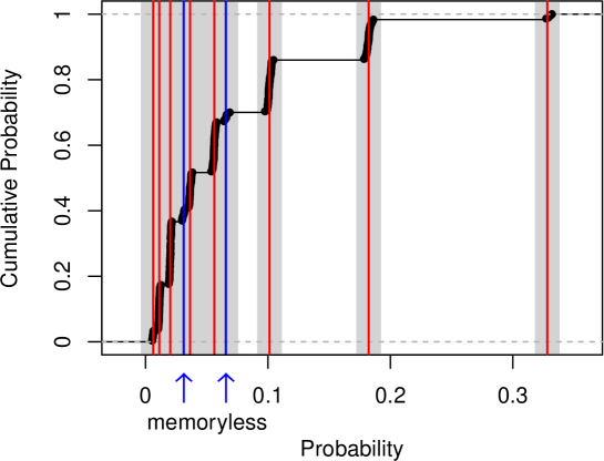
Figure 4: Empirical cumulative distribution of estimates from Algorithm 3 applied to MDP of Fig. 3.

V Smart Sampling

The simple sampling strategies used by Algorithms 2 and 3 have the disadvantage that they allocate equal simulation budget to all schedulers, regardless of their merit. In general, the problem we address has two independent components: the rarity of near optimal schedulers and the rarity of the property under a near optimal scheduler. We should allocate our simulation budget accordingly and not waste budget on schedulers that are clearly not optimal.

Motivated by the above, our smart estimation algorithm comprises three stages: (i) an initial undirected sampling experiment to discover the nature of the problem, (ii) a targeted sampling experiment to generate a candidate set of schedulers with high probability of containing an optimal scheduler and (iii) iterative refinement of the candidates to estimate the probability of the best scheduler with specified confidence. By excluding the schedulers with the worst estimated probabilities and re-allocating their simulation budget to the schedulers that remain, at each iterative step of stage (iii) the number of schedulers reduces while the confidence of their estimates increases. With a suitable choice of per-iteration budget, the algorithm is guaranteed to terminate.

In the following subsection we develop the theoretical basis of stage (ii).

V-A Maximising the Probability of Seeing a Good Scheduler

In what follows we assume the existence of an MDP and a property $\varphi$ whose probability we wish to maximise by choosing a suitable scheduler from the set $\mathfrak{S}$. Let $\mathcal{P}:\mathfrak{S}\rightarrow[0,1]$ be a function mapping schedulers to their probability of satisfying $\varphi$ and let $p_{\max}=\max_{\sigma\in\mathfrak{S}}(\mathcal{P}(s))$. For the sake of exposition, we consider the problem of finding a scheduler that maximises the probability of satisfying $\varphi$ and define a “good” (near optimal) scheduler to be one in the set $\mathfrak{S}_{g}=\{\sigma\in\mathfrak{S}\mid\mathcal{P}(\sigma)\geq p_{\max}-\varepsilon\}$ for some $\varepsilon\in(0,p_{\max}]$. Intuitively, a good scheduler is one whose probability of satisfying $\varphi$ is within $\varepsilon$ of $p_{\max}$, noting that we may similarly define a good scheduler to be one within $\varepsilon$ of $p_{\min}=\min_{\sigma\in\mathfrak{S}}(\mathcal{P}(\sigma))$, or to be in any other subset of $\mathfrak{S}$. In particular, to address reward-based MDP optimisations, a good scheduler could be defined to be the subset of $\mathfrak{S}$ that is near optimal with respect to a reward scheme. The notion of a “best” scheduler follows intuitively from the definition of a good scheduler.

If we sample uniformly from $\mathfrak{S}$, the probability of finding a good scheduler is $p_{g}=|\mathfrak{S}_{g}|/|\mathfrak{S}|$. The average probability of a good scheduler is $p_{\overline{g}}=\sum_{\sigma\in\mathfrak{S}_{g}}\mathcal{P}(\sigma)/|\mathfrak{S}_{g}|$. If we select $M$ schedulers uniformly at random and verify each with $N$ simulations, the expected number of traces that satisfy $\varphi$ using a good scheduler is thus $Mp_{g}Np_{\overline{g}}$. The probability of seeing a trace that satisfies $\varphi$ using a good scheduler is the cumulative probability

$$(1-(1-p_{g})^{M})(1-(1-p_{\overline{g}})^{N}).$$ (8)

Hence, for a given simulation budget $N_{\max}=NM$, to implement stage (ii) the idea is to choose $N$ and $M$ to maximise (8) and keep any scheduler that produces at least one trace that satisfies $\varphi$. Since, a priori, we are generally unaware of even the magnitudes of $p_{g}$ and $p_{\overline{g}}$, stage ($i$) is necessarily uninformed and we set $N=M=\lceil\sqrt{N_{\max}}\rceil$. The results of stage (i) allow us to estimate $p_{g}$ and $p_{\overline{g}}$ (see Fig. 9a) and thus maximise (8). This may be done numerically, but we have found the heuristic $N=\lceil 1/p_{\overline{g}}\rceil$ to be near optimal in all but extreme cases.

V-B Smart Estimation

Algorithm 4 is our smart estimation algorithm to find schedulers that maximise the probability of a property. The algorithm to find minimising schedulers is similar. Lines 4 to 4 implement stage (i), lines 4 to 4 implement stage (ii) and lines 4 to 4 implement stage (iii). Note that the algorithm distinguishes $p_{\max}$ (the notional true maximum probability), $p_{\overline{\max}}$ (the true probability of the best candidate scheduler found) and $\hat{p}_{\overline{\max}}$ (the estimated probability of the best candidate scheduler).

The per-iteration simulation budget $N_{\max}$ must be greater than the number needed by the standard Chernoff bound (1), to ensure that there will be sufficient simulations to guarantee the specified confidence if the algorithm refines the candidate set to a single scheduler. Typically, the per-iteration budget will be greater than this, such that the required confidence is reached before refining the set of schedulers to a single element. Under these circumstances the confidence is judged according to the Chernoff bound for multiple estimates (7). In addition, lines 4 to 4 allow the algorithm to quit as soon as the minimum number of simulations is reached.

Algorithm 4 may be further optimised by re-using the simulation results from previous iterations of stage (iii). The contribution is small, however, because confidence decreases exponentially with the age (in terms of iterations) of the results.

Input:

$\mathcal{M}$: an MDP

$\varphi$: a property

$\epsilon,\delta$: the required Chernoff bound

$N_{\max}>\ln(2/\delta)/(2\epsilon^{2})$: the per-iteration budget

Output: $\hat{p}_{\overline{\max}}\approx p_{\max}$, where $p_{\overline{\max}}\approx p_{\max}$ and $\mathrm{P}(|p_{\overline{\max}}-\hat{p}_{\overline{\max}}|\geq\epsilon)\leq\delta$

1

2$N\leftarrow\lceil\sqrt{N_{\max}}\rceil$; $M\leftarrow\lceil\sqrt{N_{\max}}\rceil$

3$S\leftarrow\{M\textnormal{ seeds chosen uniformly at random}\}$

4$\forall\sigma\in S,\forall i\in\{1,\dots,N\}:\omega_{i}^{\sigma}\leftarrow\mathrm{Simulate}(\mathcal{M},\varphi,\sigma)$

5$R:S\rightarrow\mathbb{N}$ maps scheduler seeds to number of traces satisfying $\varphi$:

$\quad R\leftarrow\{(\sigma,n)\mid\sigma\in S\wedge\mathbb{N}\ni n=\sum_{i=1}^{N}\mathbf{1}(\omega_{i}^{\sigma}\models\varphi)\}$

6$\hat{p}_{\overline{\max}}\leftarrow\max_{\sigma\in S}(R(\sigma)/N)$

7$N\leftarrow\lceil 1/\hat{p}_{\overline{\max}}\rceil$, $M\leftarrow\lceil N_{\max}\,\hat{p}_{\overline{\max}}\rceil$

8$S\leftarrow\{M\textnormal{ seeds chosen uniformly at random}\}$

9$\forall\sigma\in S,\forall i\in\{1,\dots,N\}:\omega_{i}^{\sigma}\leftarrow\mathrm{Simulate}(\mathcal{M},\varphi,\sigma)$

10$R\leftarrow\{(\sigma,n)\mid\sigma\in S\wedge\mathbb{N}\ni n=\sum_{i=1}^{N}\mathbf{1}(\omega_{i}^{\sigma}\models\varphi)\}$

11$S\leftarrow\{\sigma\in S\mid R(\sigma)>0\}$

12$\forall\sigma\in S,\;R(\sigma)\leftarrow 0$; $i\leftarrow 0$; $\mathit{conf}\leftarrow 1$

13while $\mathit{conf}>\delta\wedge S\neq\emptyset$ do

14      

15      $i\leftarrow i+1$

16      $M_{i}\leftarrow|S|$

17      $N_{i}\leftarrow 0$

18      while $\mathit{conf}>\delta\wedge N_{i}<\lceil N_{\max}/M_{i}\rceil$ do

19            

20            $N_{i}\leftarrow N_{i}+1$

21            $\mathit{conf}\leftarrow 1-(1-e^{-2\epsilon^{2}N_{i}})^{M_{i}}$

22            $\forall\sigma\in S:\omega_{N_{i}}^{\sigma}\leftarrow\mathrm{Simulate}(\mathcal{M},\varphi,\sigma)$

23      

24      $R\leftarrow\{(\sigma,n)\mid\sigma\in S\wedge\mathbb{N}\ni n=\sum_{j=1}^{N_{i}}\mathbf{1}(\omega_{j}^{\sigma}\models\varphi)\}$

25      $\hat{p}_{\overline{\max}}\leftarrow\max_{\sigma\in S}(R(\sigma)/N_{i})$

26      $R^{\prime}:\{1,\dots,|S|\}\rightarrow S$ is an injective function s.t.

       $\forall(n,\sigma),(n^{\prime},\sigma^{\prime})\in R^{\prime},\;n>n^{\prime}\implies R(\sigma)\geq R(\sigma^{\prime})$

27      $S\leftarrow\{\sigma\in S\mid\sigma=R^{\prime}(n)\wedge n\in\{\lfloor|S|/2\rfloor,\dots,|S|\}\}$

28      

29

Algorithm 4 Smart Estimating

V-C Smart Hypothesis Testing

We wish to test the hypothesis that there exists a scheduler such that property $\varphi$ has probability $\bowtie\theta$, where $\bowtie\in\{\geq,\leq\}$. Two advantages of sequential hypothesis testing are that it is not necessary to estimate the actual probability to know if an hypothesis is satisfied, and the easier the hypothesis is to satisfy, the quicker it is to get a result. Algorithm 5 maintains these advantages and uses smart sampling to improve on the performance of Algorithm 2. For the purposes of exposition, Algorithm 5 tests $H_{0}$, as described in Section II. The algorithm to test $H_{1}$ is similar.

A sub-optimal approach would be to use Algorithm 4 to refine a set of schedulers until one is found whose estimate satisfies the hypothesis with confidence according to a Chernoff bound. Our approach is to exploit the fact that the average estimate at each iteration of Algorithm 4 is known with high confidence, i.e., confidence given by the total simulation budget. This follows directly from the result of [6], where the bound is specified for a sum of arbitrary random variables, not necessarily with identical expectations. By similar arguments based on [26], it follows that the sequential probability ratio test may also be applied to the sum of results produced during the course of an iteration of Algorithm 4. Moreover, it is possible to test each scheduler with respect to its individual results and the current number of schedulers, according to the bound given in Section IV-C.

Hence, if the “average scheduler” or an individual scheduler ever satisfies the hypothesis (lines 5 and 5), the algorithm immediately terminates and reports that the hypothesis is satisfied with the specified confidence. If the “best” scheduler ever individually falsifies the hypothesis (lines 5 and 5), the algorithm also terminates and reports the result. Note that this outcome does not imply that there is no scheduler that will satisfy the hypothesis, only that no scheduler was found with the given budget. Finally, if the algorithm refines the initial set of schedulers to a single instance and the hypothesis was neither satisfied nor falsified, an inconclusive result is reported (line 5).

We implement one further important optimisation. We use the threshold probability $\theta$ to directly define the simulation budget to generate the candidate set of schedulers, i.e. $N=\lceil 1/\theta\rceil$, $M=\lceil\theta N_{\max}\rceil$ (line 5). This is justified because we need only find schedulers whose probability of satisfying $\varphi$ is greater than $\theta$. By setting $N=\lceil 1/\theta\rceil$, (8) ensures that such schedulers, if they exist, have high probability of being observed. The initial coarse exploration used in Algorithm 4 is thus not necessary.

Algorithm 5 is our smart hypothesis testing algorithm. Note that we do not set a precise minimum per-iteration simulation budget because we expect the hypothesis to be decided with many fewer simulations than would be required to estimate the probability. In practice it is expedient to initially set a low per-iteration budget (e.g., 1000) and repeat the algorithm with an increased budget (e.g., increased by an order of magnitude) if the previous test was inconclusive.

Input:

$\mathcal{M}$: an MDP

$\varphi$: a property

$H_{0}:\mathrm{P}(\omega\models\varphi)\geq\theta\pm\varepsilon$ is the hypothesis

$\alpha,\beta$: the desired error probabilities of $H_{0}$

$N_{\max}$: the per-iteration simulation budget

Output: The result of the hypothesis test

1

2Let $p^{0}=\theta+\varepsilon$, $p^{1}=\theta-\varepsilon$

3Let $A=(1-\beta)/\alpha$, $B=\beta/(1-\alpha)$

4$N\leftarrow\lceil 1/\theta\rceil$; $M\leftarrow\lceil\theta N_{\max}\rceil$

5$S\leftarrow\{M\textnormal{ seeds chosen uniformly at random}\}$

6$\forall\sigma\in S,\forall i\in\{1,\dots,N\}:\omega_{i}^{\sigma}\leftarrow\mathrm{Simulate}(\mathcal{M},\varphi,\sigma)$

7$R\leftarrow\{(\sigma,n)\mid\sigma\in S\wedge\mathbb{N}\ni n=\sum_{i=1}^{N}\mathbf{1}(\omega_{i}^{\sigma}\models\varphi)\}$

8if $\frac{(p^{1})^{\sum R(\sigma)}(1-p^{1})^{N_{\max}-\sum R(\sigma)}}{(p^{0})^{\sum R(\sigma)}(1-p^{0})^{N_{\max}-\sum R(\sigma)}}\leq A$ then

9      Accept $H_{0}$ and quit

10

11$S\leftarrow\{\sigma\in S\mid R(\sigma)>0\}$, $M\leftarrow|S|+1$

12while $M>1$ do

13      

14      $M\leftarrow|S|$

15      Let $\alpha_{M}=1-\sqrt[M]{1-\alpha}$, $\beta_{M}=1-\sqrt[M]{1-\beta}$

16      Let $A_{M}=(1-\beta_{M})/\alpha_{M}$, $B_{M}=\beta_{M}/(1-\alpha_{M})$

17      Let $\mathit{ratio}=1$

18      for $\sigma_{i}\in S,i\in\{1,\dots,M\}$ do

19            

20            Let $\mathit{ratio}_{i}=1$

21            for $j\in\{1,\dots,N\}$ do

22                  

23                  $\omega\leftarrow\mathrm{Simulate}(\mathcal{M},\varphi,\sigma_{i})$

24                  if $\omega\models\varphi$ then

25                        

26                        $\mathit{ratio}\leftarrow\frac{p_{1}}{p_{0}}\mathit{ratio}$; $\mathit{ratio}_{i}\leftarrow\frac{p_{1}}{p_{0}}\mathit{ratio}_{i}$

27                  else

28                        

29                        $\mathit{ratio}\leftarrow\frac{1-p_{1}}{1-p_{0}}\mathit{ratio}$; $\mathit{ratio}_{i}\leftarrow\frac{1-p_{1}}{1-p_{0}}\mathit{ratio}_{i}$

30                  if $\mathit{ratio}\leq A\vee\mathit{ratio}_{i}\leq A_{M}$ then

31                        

32                        Accept $H_{0}$ and quit

33                  if $\mathit{ratio}_{i}\geq B_{M}$ then

34                        

35                        Reject $H_{0}$ (given budget) and quit

36                  

37            

38      

39      $R^{\prime}:\{1,\dots,|S|\}\rightarrow S$ is an injective function s.t.

      $\forall(n,\sigma),(n^{\prime},\sigma^{\prime})\in R^{\prime},\;n>n^{\prime}\implies R(\sigma)\geq R(\sigma^{\prime})$

40      $S\leftarrow\{\sigma\in S\mid\sigma=R^{\prime}(n)\wedge n\in\{\lfloor|S|/2\rfloor,\dots,|S|\}\}$

41Inconclusive result (given budget)

42

Algorithm 5 Smart Hypothesis Testing

VI Case Studies

To demonstrate the performance of smart sampling, we have implemented Algorithms 4 and 5 in our statistical model checking platform Plasma [5]. We performed a number of experiments on standard models taken from the numerical model checking literature, most of which can be found illustrated on the Prism website. We found that all of our estimation experiments achieved their specified Chernoff bounds ($\varepsilon=\delta=0.01$ in all cases) with a relatively modest per-iteration simulation budget of $10^{5}$ simulations. The actual number of simulation cores used for the estimation results was subject to availability and varied between experiments. To facilitate comparisons, in what follows we normalise all timings to be with with respect to 64 cores. Typically, each data point was produced in a few tens of seconds. Our hypothesis tests were performed on a single machine, without distribution. Despite this, most experiments completed in just a few seconds (some in fractions of a second), demonstrating that our smart hypothesis testing algorithm is able to take advantage of easy hypotheses.

VI-A IEEE 802.11 Wireless LAN Protocol

We consider a reachability property of the IEEE 802.11 Wireless LAN (WLAN) protocol model of [20]. The protocol aims to avoid “collisions” between devices sharing a communication channel, by means of an exponential backoff procedure when a collision is detected. We therefore estimate the probability of the second collision at various time steps, using Algorithm 4 with per-iteration budget of $10^{5}$ simulations. Fig. 5 illustrates the estimated maximum probabilities ($\hat{p}_{\max}$) and minimum probabilities ($\hat{p}_{\min}$) for time steps $k\in\{0,10,\dots,100\}$. The property is expressed as $\mathbf{F}^{k}col=2$. The shaded areas indicate the true probabilities $\pm 0.01$, the specified absolute error bound using Chernoff bound $\varepsilon=\delta=0.01$. Our results are clearly very close to the true values. Table I gives the results of hypothesis tests based on the same model using property $\mathbf{F}^{100}col=2$. See Section VI-B for a description.

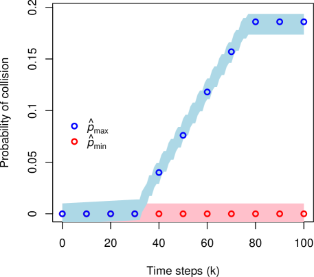
Figure 5: Estimated maximum and minimum probabilities of second collision in WLAN protocol. Shaded regions denote true values $\pm 0.01$.

The results illustrated in Fig. 5 refer to the same property and confidence as the those shown in Fig. 4 of [22]. The total simulation cost to generate a point in Fig. 5 is $1.2\times 10^{6}$ (12 iterations of $10^{5}$ simulations using smart sampling), compared to a cost of $2.7\times 10^{8}$ per point in Fig. 4 of [22] (4000 schedulers tested with 67937 simulations using simple sampling). This demonstrates a more than 200-fold improvement in performance.

VI-B IEEE 802.3 CSMA/CD Protocol

The IEEE 802.3 CSMA/CD protocol is a wired network protocol that is similar in operation to that of IEEE 802.11, but using collision detection instead of collision avoidance. In Table I we give the results of applying Algorithm 5 to the IEEE 802.3 CSMA/CD protocol model of [18]. The models and parameters are chosen to compare with results given in Table III in [11], hence we also give results for hypothesis tests performed on the WLAN model used in Section VI-A. In contrast to the results of [11], our results are produced on a single machine, with no parallelisation. There are insufficient details given about the experimental conditions in [11] to make a formal comparison (e.g., error probabilities of the hypothesis tests and number of simulation cores), but it seems that the performance of our algorithm is generally much better. We set $\alpha=\beta=\delta=0.01$, which constitute a fairly tight bound, and note that, as expected, the simulation times tend to increase as the threshold $\theta$ approaches the true probability.

CSMA 3 4	$\theta$	0.5	0.8	0.85	0.86	0.9	0.95
	time	0.5	3.5	737	*	2.9	2.5
CSMA 3 6	$\theta$	0.3	0.4	0.45	0.48	0.5	0.8
	time	1.3	5.2	79	*	39	2.6
CSMA 4 4	$\theta$	0.5	0.7	0.8	0.9	0.93	0.95
	time	0.2	0.3	4.0	8.6	*	3.8
WLAN 5	$\theta$	0.1	0.15	0.18	0.2	0.25	0.5
	time	0.8	2.6	*	2.9	2.9	1.3
WLAN 6	time	1.3	2.2	*	6.5	1.3	1.3

Table I: Hypothesis test results for CSMA/CD and WLAN protocols. $\theta$ is the threshold probability or the true probability (marked by asterisk). time is simulation time in seconds to achieve the correct result on a single machine.

VI-C Choice Coordination

To demonstrate the scalability of our approach, we consider the choice coordination model of [23] and estimate the minimum probability that a group of six tourists will meet within $T$ steps. The model has a parameter ($\mathit{BOUND}$) that limits the state space. We set $\mathit{BOUND}=100$, making the state space of $\approx 5\times 10^{16}$ states intractable to numerical model checking. Fortunately, it is possible to infer the correct probabilities from tractable parametrisations. For $T=20$ and $T=25$ the true minimum probabilities are respectively $0.5$ and $0.75$. Using smart sampling and a Chernoff bound of $\varepsilon=\delta=0.01$, we correctly estimate the probabilities to be $0.496$ and $0.745$ in a few tens of seconds on 64 simulation cores.

VI-D Network Virus Infection

Network virus infection is a subject of increasing relevance. Hence, using a per-iteration budget of $10^{5}$ simulations, we demonstrate the performance of Algorithm 4 on the Prism virus infection case study based on [19]. The network is illustrated in Fig. 2 and comprises three sets of linked nodes: a set of nodes containing one infected by a virus, a set of nodes with no infected nodes and a set of barrier nodes which divides the first two sets. A virus chooses which node to infect nondeterministically. A node detects a virus probabilistically and we vary this probability as a parameter for barrier nodes. We consider time as a second parameter. Figs. 6 and 7 illustrate the estimated probabilities that the target node in the uninfected set will be infected. We observe in Figs. 6b and 7b that the estimated minimums are within $[-0.0070,+0.00012]$ and the estimated maximums are within $[-0.00012,+0.0083]$ of their true values. The respective negative and positive biases to these error ranges reflects the fact that Algorithm 4 converges from respectively below and above (as illustrated in Fig. 9b). The average time to generate a point in Fig. 6 was approximately 100 seconds, using 64 simulation cores. Points in Fig. 7 took on average approximately 70 seconds.

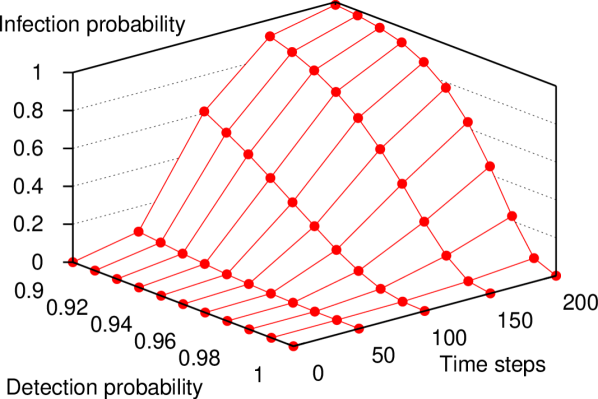
(a) Estimates.

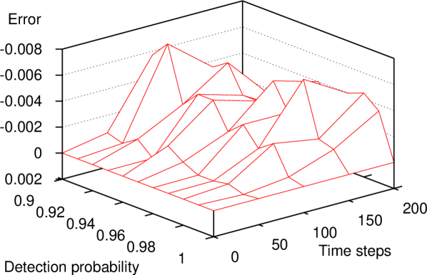
(b) Errors.

Figure 6: Minimum probability of network infection.

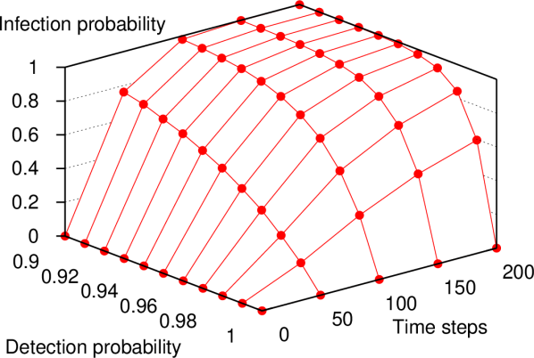
(a) Estimates.

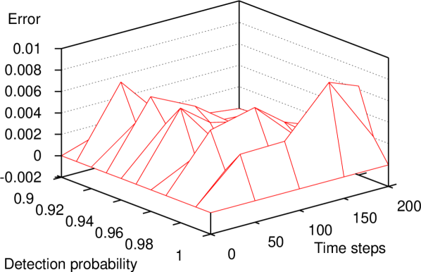
(b) Errors.

Figure 7: Maximum probability of network infection.

VI-E Gossip Protocol

Gossip protocols are an important class of network algorithms that rely on local connectivity to propagate information globally. Using the gossip protocol model of [17], we used Algorithm 4 with per-simulation budget of $10^{5}$ simulations to estimate the maximum ($\hat{p}_{\max}$) and minimum ($\hat{p}_{\min}$) probabilities that the maximum path length between any two nodes is less than 4 after $T$ time steps. This is expressed by property $\mathbf{F}^{T}\mathit{max\_path\_len}<4$. The results are illustrated in Fig. 8. Estimates of maximum probabilities are within $[-0,+0.0095]$ of the true values. Estimates of minimum probabilities are within $[-0.007,+0]$ of the true values. Each point in the figure took on average approximately 60 seconds to generate using 64 simulation cores.

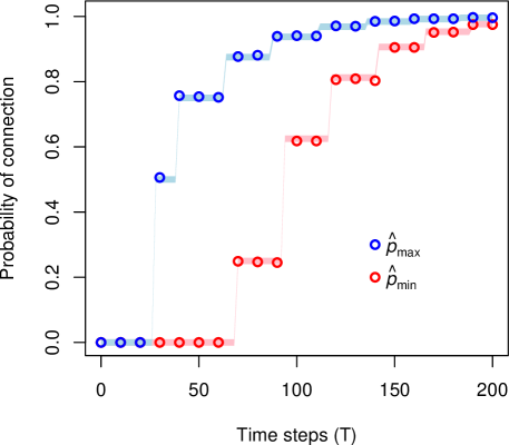
Figure 8: Estimated probabilities that maximum path length is $<4$ in gossip protocol model. Shaded regions denote $\pm 0.01$ of true values.

VII Convergence and Counterexamples

The techniques described in the preceding sections open up the possibility of efficient lightweight verification of MDPs, with the consequent possibility to take full advantage of parallel computational architectures, such as multi-core processors, clusters, grids, clouds and general purpose computing on graphics processors (GPGPU). These architectures may potentially divide the problem by the number of available computational devices (i.e., linearly), however this must be considered in the context of scheduler space increasing exponentially with path length. Although Monte Carlo techniques are essentially impervious to the size of the state space (they also work with non-denumerable space), it is easy to construct verification problems for which there is a unique optimal scheduler. Such examples do not necessarily invalidate the approach, however, because it may not be necessary to find the possibly unique optimal scheduler to return a result with a level of statistical confidence. The nature of the distribution of schedulers nevertheless affects efficiency, so in this section we explore the convergence properties of smart sampling and give an example from the literature that does not converge as well as the case studies in Section VI.

Essentially, the problem is that of exponentially distributed schedulers, i.e., having a very low mass of schedulers close to the optimum. Fig. 11 illustrates the difference between exponentially decreasing and linearly decreasing distributions with the same overall mass. In both cases $p_{\max}\approx 0.2$ (the density at 0.2 is zero), but the figure shows that there is more probability mass near 0.2 in the case of the linear distribution.

Figure 9 illustrates the convergence of Algorithm 4, using a per-iteration budget of $10^{6}$ applied to schedulers whose probability of success (i.e., of satisfying a hypothetical property) is distributed according to the exponential distribution of Fig. 11. Fig. 9a shows how the initial undirected sampling (black dots) crudely approximates $p_{\max}$. This approximation is then used to generate the candidate set of schedulers (red distribution). The black lines illustrate five iterations of refinement, resulting in a shift of the distribution towards $p_{\max}$. Fig. 9b illustrates the same shift in terms of the convergence of probabilities. Iteration 0 corresponds to the undirected sampling. Iteration 1 corresponds to the generation of the candidate set of schedulers. Note that for these first two iterations, $\hat{p}_{\mathrm{mean}}$ includes schedulers that have zero probability of success. The expected value of $\hat{p}_{\mathrm{mean}}$ in these two iterations is equal to the expected probability obtained by the uniform probabilistic scheduler. This fact can be used to verify that the hash function and PRNG described in Section IV sample uniformly. In subsequent iterations the candidates all have non-zero probability of success. Importantly, the figure demonstrates that there is a significant increase in the maximum probability of scheduler success ($\sigma_{\max}$) between iteration 0 and iteration 1, and that this maximum is maintained throughout the subsequent refinements. Despite the apparently very low density of schedulers near $p_{\max}$, Algorithm 4 is able to make a good approximation.

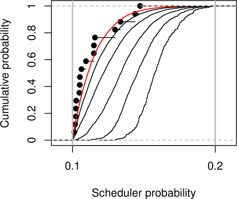
(a) Scheduler distributions. Dots denote the results of initial sampling. The red line is the set of schedulers to refine. Black lines show the result of subsequent refinements.

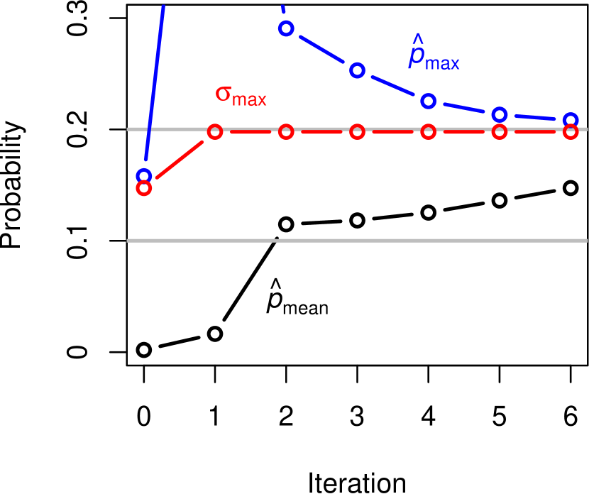
(b) Estimates and schedulers. At each iterative step: $\hat{p}_{\max}$ is the maximum estimate, $\hat{p}_{\mathrm{mean}}$ is the mean estimate and $\sigma_{\max}$ is the true maximum probability of the available schedulers.

Figure 9: Convergence of Algorithm 4 with exponentially distributed scheduler probabilities (Fig. 11) and per-iteration budget of $10^{6}$ simulations.

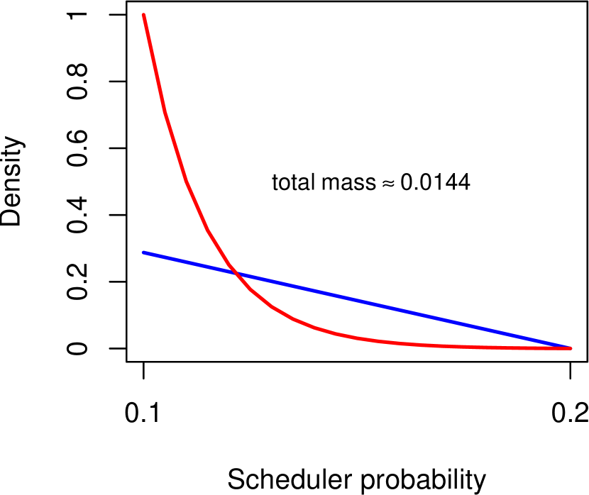
Figure 10: Theoretical linear (blue) and exponential (red) scheduler densities with probability mass $\approx 0.0144$ and zero density at probability 0.2.

Figure 11: Performance of smart sampling (black dots) applied to self-stabilising models of [13]. Red shaded areas denote true values $\pm 0.01$.

The theoretical performance demonstrated in Fig. 9 explains why we are able to achieve good results in Section VI. It is nevertheless possible to find examples for which accurate results are difficult to achieve. Fig. 11 illustrates the results of applying Algorithm 4 to instances of the self-stabilising algorithm of [13], using a per-iteration budget of $10^{5}$. Although the estimates (black dots) do not lie within our statistical confidence bounds of the true values (red shaded areas), we nevertheless claim that the results are useful. The problem of quantifying the confidence of estimates with respect to optimal values remains open, however.

To improve the performance of smart sampling, it is possible to make an even better allocation of simulation budget. For example, if good schedulers are very rare it may be beneficial to increase the per-iteration budget (thus increasing the possibility of seeing a good scheduler in the initial candidate set) but increase the proportion of schedulers rejected after each iteration (thus reducing the overall number of iterations and maintaining a fixed total number of simulations). To avoid rejecting good schedulers under such a regime, it may be necessary to reject fewer schedulers in the early iterations when confidence is low.

VIII Prospects and Challenges

The use of sampling facilitates algorithms that scale independently of the sample space, hence we anticipate that it will be possible to apply our techniques to nondeterministic models with non-denumerable schedulers. We believe it is immediately possible to apply smart sampling to reward-based MDP optimisation problems.

The success of sampling depends on the relative abundance of near optimal schedulers in scheduler space and our experiments suggest that these are not rare in standard case studies. While it is possible to construct pathological examples, where near optimal schedulers cannot easily be found by sampling, it is perhaps even simpler to confound numerical techniques with state explosion (three independent counters ranging over 0 to 1000 is typically sufficient with current hardware). Hence, as with numerical model checking, our ongoing challenge is essentially to increase performance and increase the number of models and problems that may be efficiently addressed. Smart sampling has made significant improvements over simple sampling, but we recognise that it will be necessary to develop other techniques to accelerate convergence. We anticipate that the most fruitful approaches will be (i) to reduce the sampled scheduler space to only those that satisfy the property and (ii) to construct schedulers piecewise. Such techniques will also reduce the potential of hash function collisions.

An important remaining challenge is to quantify the confidence of our estimates and hypothesis tests with respect to optimality. In the case of hypothesis tests that satisfy the hypothesis, the statistical confidence of the result is sufficient. If an hypothesis is not satisfied, however, the statistical confidence does not relate to whether there exists a scheduler to satisfy it. Likewise, the statistical confidence bounds of probability estimates imply nothing about how close they are to the true optima. We nevertheless know that our estimates of the extrema must lie within the true extrema or exceed them with the specified statistical confidence. This is already useful and a significant improvement over the results produced using the uniform probabilistic scheduler. In addition, given the number of simulations performed, we may at least quantify confidence with respect to the product $p_{g}p_{\overline{g}}$ (the rarity of near optimal schedulers times the average probability of the property with near optimal schedulers).

References

- [1] Christel Baier and Joost-Pieter Katoen. Principles of model checking. MIT Press, 2008.
- [2] Richard Bellman. Dynamic Programming. Princeton University Press, 1957.
- [3] Andrea Bianco and Luca De Alfaro. Model checking of probabilistic and nondeterministic systems. In Foundations of Software Technology and Theoretical Computer Science, pages 499–513. Springer, 1995.
- [4] Jonathan Bogdoll, Luis María Ferrer Fioriti, Arnd Hartmanns, and Holger Hermanns. Partial order methods for statistical model checking and simulation. In Formal Techniques for Distributed Systems, pages 59–74. Springer, 2011.
- [5] Benoît Boyer, Kevin Corre, Axel Legay, and Sean Sedwards. PLASMA-lab: A flexible, distributable statistical model checking library. In Kaustubh Joshi, Markus Siegle, Mariëlle Stoelinga, and PedroR. D’Argenio, editors, Quantitative Evaluation of Systems, volume 8054 of LNCS, pages 160–164. Springer, 2013.
- [6] Herman Chernoff. A measure of asymptotic efficiency for tests of a hypothesis based on the sum of observations. Ann. Math. Statist., 23(4):493–507, 1952.
- [7] E.M. Clarke, E. A. Emerson, and J. Sifakis. Model checking: algorithmic verification and debugging. Commun. ACM, 52(11):74–84, November 2009.
- [8] Thomas H. Cormen, Charles E. Leiserson, Ronald L. Rivest, and Clifford Stein. Introduction to Algorithms. MIT Press, 3rd edition, 2009.
- [9] Hans Hansson and Bengt Jonsson. A logic for reasoning about time and reliability. Formal aspects of computing, 6(5):512–535, 1994.
- [10] Arnd Hartmanns and Mark Timmer. On-the-fly confluence detection for statistical model checking. In NASA Formal Methods, pages 337–351. Springer, 2013.
- [11] David Henriques, Joao G. Martins, Paolo Zuliani, André Platzer, and Edmund M. Clarke. Statistical model checking for Markov decision processes. In Quantitative Evaluation of Systems, 2012 Ninth International Conference on, pages 84–93. IEEE, 2012.
- [12] William George Horner. A new method of solving numerical equations of all orders, by continuous approximation. Philosophical Transactions of the Royal Society of London, 109:308–335, 1819.
- [13] A. Israeli and M. Jalfon. Token management schemes and random walks yield self-stabilizating mutual exclusion. In Proc. 9th Annual ACM Symposium on Principles of Distributed Computing (PODC ’90), pages 119–131. ACM New York, 1990.
- [14] Michael Kearns, Yishay Mansour, and Andrew Y. Ng. A sparse sampling algorithm for near-optimal planning in large Markov decision processes. Machine Learning, 49(2-3):193–208, 2002.
- [15] Donald E. Knuth. The Art of Computer Programming. Addison-Wesley, 3rd edition, 1998.
- [16] M. Kwiatkowska, G. Norman, and D. Parker. Stochastic model checking. In M. Bernardo and J. Hillston, editors, Formal Methods for the Design of Computer, Communication and Software Systems: Performance Evaluation (SFM’07), volume 4486 of LNCS (Tutorial Volume), pages 220–270. Springer, 2007.
- [17] Marta Kwiatkowska, Gethin Norman, and David Parker. Analysis of a gossip protocol in PRISM. SIGMETRICS Perform. Eval. Rev., 36(3):17–22, November 2008.
- [18] Marta Kwiatkowska, Gethin Norman, David Parker, and Jeremy Sproston. Performance analysis of probabilistic timed automata using digital clocks. Formal Methods in System Design, 29:33–78, August 2006.
- [19] Marta Kwiatkowska, Gethin Norman, David Parker, and Maria Grazia Vigliotti. Probabilistic mobile ambients. Theoretical Computer Science, 410(12-13):1272–1303, 2009.
- [20] Marta Z. Kwiatkowska, Gethin Norman, and Jeremy Sproston. Probabilistic model checking of the IEEE 802.11 wireless local area network protocol. In Proc. Joint International Workshop on Process Algebra and Probabilistic Methods, Performance Modeling and Verification, pages 169–187. Springer, 2002.
- [21] Richard Lassaigne and Sylvain Peyronnet. Approximate planning and verification for large Markov decision processes. In Proc. Annual ACM Symposium on Applied Computing, pages 1314–1319. ACM, 2012.
- [22] A. Legay, S. Sedwards, and L.-M. Traonouez. Scalable verification of Markov decision processes. In 4th Workshop on Formal Methods in the Development of Software (FMDS 2014), LNCS. Springer, 2014.
- [23] U. Ndukwu and A. McIver. An expectation transformer approach to predicate abstraction and data independence for probabilistic programs. In Proc. 8th Workshop on Quantitative Aspects of Programming Languages (QAPL’10), 2010.
- [24] Masashi Okamoto. Some inequalities relating to the partial sum of binomial probabilities. Annals of the Institute of Statistical Mathematics, 10(1):29–35, 1958.
- [25] Martin L. Puterman. Markov Decision Processes: Discrete Stochastic Dynamic Programming. Wiley-Interscience, 1994.
- [26] Abraham Wald. Sequential tests of statistical hypotheses. The Annals of Mathematical Statistics, 16(2):117–186, 1945.
- [27] Douglas J. White. Real applications of Markov decision processes. Interfaces, 15(6):73–83, 1985.
- [28] Douglas J. White. Further real applications of Markov decision processes. Interfaces, 18(5):55–61, 1988.
- [29] Douglas J. White. A survey of applications of Markov decision processes. Journal of the Operational Research Society, 44(11):1073–1096, Nov. 1993.
- [30] H. L. S. Younes. Verification and Planning for Stochastic Processes with Asynchronous Events. PhD thesis, Carnegie Mellon University, 2005.
- [31] Håkan L. S. Younes and Reid G. Simmons. Probabilistic verification of discrete event systems using acceptance sampling. In Computer Aided Verification, pages 223–235. Springer, 2002.