Maximum probability domains for the analysis of the microscopic structure of liquids

Abstract

We introduce the concept of maximum probability domains (MPDs), developed in the context of the analysis of electronic densities, in the study of the microscopic spatial structures of liquids. The idea of locating a particle in a three dimensional region, by determining the domain where the probability of finding that, and only that, particle is maximum, gives an interesting characterization of the local structure of the liquid. The optimization procedure, required for the search of the domain of maximum probability, is carried out by the implementation of the level set method. Results for a couple of case studies are presented, to illustrate the structure of liquid water at ambient conditions and upon increasing pressure from the point of view of MPDs and to compare the information encoded in the solvation shells of sodium in water with, once again, that extracted from the MPDs.

I Introduction

While liquids have long-range disorder, they exhibit a local order that drives many of their physical properties. This short-range order is usually characterized through the Radial Distribution Functions (RDFs) Hansen and McDonald (1986). However, the RDFs convey little or indirect information about the three-dimensional (3D) local structure of liquids. Spatial Distribution Functions (SDFs) have then been introduced for this purpose Svishchev and Kusalik (1993); Daub et al. (2009). Since then, several indicators of the local order of liquids have been proposed, in particular for the important case of liquid water, including the statistics of Voronoi polyhedron Shih et al. (1994); Jedlovszky (1999); Chakraborty and Chandra (2011); Stirnemann and Laage (2012); Idrissi et al. (2013), local structure index Errington and Debenedetti (2001) or angular correlation Saitta and Datchi (2003); Babiaczyk et al. (2010). Recently, local density fluctuations and the probability distribution of occupancy of a given volume have attracted a lot of attention, in the framework of the theory of hydrophobicity Chandler (2005). These have been used to characterize and locate patches of hydrophobicity or hydrophilicity at surfaces Acharya et al. (2010); Patel et al. (2011); Rotenberg et al. (2011) or around proteins Acharya et al. (2010); Patel and Garde (2014). However, as such, they have not been used to characterize the microscopic structure of liquids.

In a very different context, that of electronic structure, related concepts have been used to locate electron pairs Cancès et al. (2004); Francisco et al. (2007); Pendás et al. (2007). In general, these methods are designed to identify regions in 3D space with particular chemical and physical meaning. The analysis is based on the information provided by the electronic probability density calculated from the many-body wave function, but offers a way to define and to visualize some relevant regions in real space.

The work presented in this paper is motivated by the interest for developing an alternative approach to study the local structure of liquid systems, combined with the clear similarities between the electronic probability density and the atomic many-body probability distribution of a liquid. We propose here a method based on the identification of regions of space where the probability of finding one and only one particle is maximum. We refer to these regions as Maximum Probability Domains (MPDs). The definition of this probability is given as the generalization of the concept Cancès et al. (2004); Gallegos et al. (2005); Scemama et al. (2007); Causà and Savin (2011); Lopes Jr et al. (2012) used for the analysis of electronic probability densities in molecules and indeed can be generalized to the case of $n$ (and only $n$) particles. The information encoded in this quantity has a many-body nature, also when considering the one-particle occupancy probability. It has to be viewed as the probability of finding $n$ particles within a certain region of space with all other particles outside. Therefore, such probability is different from any reduced $n$-particle probability density, since the degrees of freedom of the $N-n$ remaining particles ($N$ being the total number of particles in the system) are not integrated out. In analogy to such quantities, however, the probability can be evaluated by using a standard sampling procedure with Molecular Dynamics (MD) or Monte Carlo (MC) trajectories.

We illustrate the method by applying it to describe the structure of pure liquid water and to define the solvation shells of sodium ions in a diluted water solution. We compare the results of our study with more standard approaches based on the RDFs and with various definitions of solvation shells. It will become apparent from the illustrations that the method offers an efficient complementary tool to the analysis of liquid structures, both qualitatively and quantitatively. The one-particle MPD defines the boundary of the 3D region available to a given particle, where it is not likely that another particle can penetrate. When a set of MPDs is identified around a central water molecule or sodium ion, we obtain a 3D-map of the locations of the surrounding molecules with a number of MPDs that is usually smaller, as we will see later, than the standard coordination number. The request of exclusive occupation of a MPD by only one particle is responsible for this feature, even though for rigid local structures, as the first solvation shell of water, there are clear similarities between the two pictures (MPDs and coordination numbers).

The results for liquid water at different densities are mainly presented as a test case, in order to prove that the method is able to recover known results even if the problem is analyzed from a new perspective. A more challenging application is represented by the case of sodium in water. Here, the one-particle MPDs located around the central ion are organized such that the spherical symmetry of the problem is maintained. However, the shape and dimension of the domains give a 3D resolution that is not accessible, or at least not directly, when employing the SDFs. We find relevant to stress here that, as will become clear from the applications, the major strength of the method developed in the paper is not to be searched in a new overall picture of the liquid achieved by determining the MPDs. The details are what make this method an interesting alternative or complement to more standard analysis techniques. Being able to pinpoint the location of the interstitial water molecules that are mainly affected by the increase of the density in liquid water or analyzing the shape of the regions occupied by water around a central molecule or ion could be used to predict properties such as the life-time of a H-bond or the kinetic of a reaction. These developments will not be discussed here, since our major goal is establishing the theoretical basis of the method and proving its efficiency with a few illustrations.

The paper is organized as follows. In Section II, we introduce the general definition of the one-particle occupancy probability. Then, the maximization of such probability is posed as a geometric optimization problem and solved within the framework of the Level Set Method (LSM) in Section III. Section IV gives the details for the numerical implementation of the method and we present the two illustrations mentioned before in Section V. Finally, in Section VI we conclude and state our outlook for future developments.

II Definition of Maximum Probability Domains

The one-particle Maximum Probability Domain (MPD) is defined as the region in three-dimensional (3D) space where the probability of finding one, and only one, particle is maximum. In the present context, the term particle stands for an atom or the center of mass of a molecule or some other point of high symmetry in a molecule. The choice depends on the information that we want to extract from this analysis. For instance, in the study of liquid water, as presented in this paper, the particles will be the oxygen atoms in the molecules.

If a system is composed of $N+1$ identical particles with positions ${\mathbf{R}^{\prime}}^{N+1}=\mathbf{R}_{0}^{\prime},\mathbf{R}_{1}^{\prime},\ldots,\mathbf{R}_{N}^{\prime}$ and we focus on the $N$ particles with positions $\mathbf{R}_{i}=\mathbf{R}_{i}^{\prime}-\mathbf{R}_{0}^{\prime}$ for $i=1,\ldots N$, we can define the one-particle occupancy probability of a domain $\Delta$, $P^{(1)}(\Delta)$, as the probability of finding one, and only one, particle in the region of space $\Delta$ with all other particles located outside $\Delta$. This probability Scemama et al. (2007), written as

$$P^{(1)}(\Delta)=\sum_{i=1}^{N} \int_{\Delta_{c}}d\mathbf{R}_{1}\ldots d\mathbf{R}_{i-1}\int_{\Delta}d\mathbf{R}_{i}\int_{\Delta_{c}}d\mathbf{R}_{i+1}\ldots d\mathbf{R}_{N}\,\rho(\mathbf{R}^{N}),$$ (1)

is what in mathematics is called a set function. Here, $\rho(\mathbf{R}^{N})$ is the configurational probability density and, in the particular case of water and sodium diluted in water, will be explicitly defined in Appendix A.

The domain $\Delta$ is given in a reference frame that is centered on the particle at $\mathbf{R}_{0}^{\prime}$, which is kept out of statistics (in the sense that in Eq. (1) we do not integrate over its positions). $\Delta_{c}$ is the symbol used to indicate the complementary volume of $\Delta$. The sum in Eq. (1) allows us to define the probability that is independent of the identity of the particle occupying the domain $\Delta$. Moreover, the notation in Eq. (1) indicates that all integrals involving the variables $\mathbf{R}_{1}\ldots\mathbf{R}_{i-1}$ and $\mathbf{R}_{i+1}\ldots\mathbf{R}_{N}$ are performed over $\Delta_{c}$. This definition of the probability can be easily extended to $n$ particles in $\Delta$ and $N-n$ particles in $\Delta_{c}$. Eq. (1) satisfies the normalization condition

$$\sum_{n=0}^{N}P^{(n)}(\Delta)=1,$$ (2)

which can be easily obtained for an ideal gas (in the absence of interactions among particles) occupying a volume $V$, as the configurational probability density is explicitly known, i.e. $\rho(\mathbf{R}^{N})=V^{-N}$, thus allowing for the analytic calculation of Eq. (1). This is done by inserting the expression of the one-particle occupancy probability $P^{(n)}(\Delta)=\binom{N}{n}v^{n}(V-v)^{N-n}/V^{N}$ in Eq. (2), where $v$ is the volume occupied by $\Delta$ and $V-v$ that occupied by $\Delta_{c}$.

To extend the integration domain in Eq. (1) to the whole configuration space, we introduce the characteristic function $\Upsilon_{\Delta}(\mathbf{R})$, defined as

$$\Upsilon_{\Delta}(\mathbf{R})=\left\{\begin{array}[]{ll}1&\mbox{if}\,\,\mathbf{R}\in\Delta\\ 0&\mbox{otherwise}\end{array}\right.,\quad\Upsilon_{\Delta_{c}}(\mathbf{R})=1-\Upsilon_{\Delta}(\mathbf{R}).$$ (3)

The probability $P^{(1)}(\Delta)$ is then

$$P^{(1)}(\Delta)=\sum_{i=1}^{N}\int d\mathbf{R}^{N}\Upsilon_{\Delta}(\mathbf{R}_{i})\prod_{j\neq i}^{N}\left(1-\Upsilon_{\Delta}(\mathbf{R}_{j})\right)\rho(\mathbf{R}^{N})$$ (4)

which allows us to identify the microscopic observable

$$\Gamma_{\Delta}^{(i)}(\mathbf{R}^{N})=\Upsilon_{\Delta}(\mathbf{R}_{i})\prod_{j\neq i}^{N}\left(1-\Upsilon_{\Delta}(\mathbf{R}_{j})\right).$$ (5)

The equilibrium average of $\Gamma_{\Delta}^{(i)}(\mathbf{R}^{N})$, evaluated according to the probability density $\rho(\mathbf{R}^{N})$, leads to the definition of $P^{(1)}(\Delta)$

$$P^{(1)}(\Delta)=\left\langle\sum_{i=1}^{N}\Gamma_{\Delta}^{(i)}\left(\mathbf{R}^{N}\right)\right\rangle.$$ (6)

Eq. (6) can be evaluated by sampling the microscopic observable $\Gamma_{\Delta}^{(i)}(\mathbf{R}^{N})$ along a Molecular Dynamics (MD) or Monte Carlo (MC) trajectory. From the algorithmic point of view, $P^{(1)}(\Delta)$ can be estimated by computing

$$\nu^{(1)}(\Delta)=\frac{1}{N_{conf}}\sum_{\kappa=1}^{N_{conf}}\delta_{1,n_{\Delta}(\kappa)}\simeq P^{(1)}(\Delta),$$ (7)

the frequency of the event “one, and only one, particle inside $\Delta$”. Here, $N_{conf}$ is the total number of configurations sampled along the trajectory and $\kappa$ labels the selected configuration. The term in the sum is equal to one only if the number of particles $n_{\Delta}(\kappa)$ inside the volume $\Delta$, for the configuration $\kappa$, is equal to 1.

The construction of the MPDs is carried out by initially choosing some centers around the central particle (labeled by 0) and some volumes enclosing these centers. A set of MPDs will be then identified as

$$\Delta^{*}_{i}=\arg\max_{\Delta_{i}}P^{(1)}(\Delta_{i}),\quad\mbox{with}\,\,i=1,2,\ldots.$$ (8)

The centers around the 0th particle can be chosen quite arbitrarily, however we find useful to locate them in correspondence of the local maxima of the Spatial Distribution Function (SDF) or of the Radial Distribution Function (RDF). It is worth underlining that $\Delta^{*}_{i}$ is not an absolute maximum  over all space of volumes, but it is the one found by a local search (the closest to the initial choice).

The definition of the set of MPDs $\Delta_{1}^{*},\Delta_{2}^{*},\ldots$ can be used for the characterization of the structure of atomic and molecular liquids as an alternative or a complement to standard tools such as distribution functions, solvation shells and coordination numbers. The determination of the optimized domains $\Delta^{*}_{i}$’s is posed as a geometric optimization problem, since the probability $P^{(1)}(\Delta_{i})$ has to be maximized with respect to variations of $\Delta_{i}$. In the following section we present He et al. (2007); Mohammadi and Pironneau (2002); Allaire et al. (2004); Grinfeld (2010); Osher and Sethian (1988) the Level Set Method (LSM) to be applied in the search of the MPDs, in particular in a liquid.

III Shape derivative in the level set method

A central concept in the procedure referred to as LSM is that of shape derivative. The function $P^{(1)}(\Delta)$ belongs to a specific class of what is normally called a set function and the variations of a set function with respect to changes of the set define its shape derivative. The aim of the numerical procedure developed and tested in this paper is to determine how $P^{(1)}(\Delta)$ changes by varying $\Delta$, such that the value of the probability itself is maximized. Appendix B is devoted to a detailed discussion on the shape derivative and on its expression in the context of the MPDs. Here, we will focus on illustrating the essence of such concept.

The set function defined in Eq. (1) depends on the integration volume, $\Delta$. Therefore, when $\Delta$ changes, also the value of the integral performed over $\Delta$ changes: such (infinitesimail) variations of $P^{(1)}(\Delta)$ will be indicated with the symbol $\mathcal{D}_{S}P^{(1)}(\Delta)$, the shape derivative. In the particular application discussed here, we request that this variation of the integration domain follows a well-defined law: The value of the integral has to increase as $\Delta$ is varied. This choice of variation allows us to define a deformation law, namely a fictitious equation of motion such as

$$\Delta\rightarrow\Delta_{\tau}=\left\{\mathbf{R}_{\tau}=\mathbf{R}+\mathbf{v}(\mathbf{R})d\tau\,|\,\mathbf{R}\in\partial\Delta\right\},$$ (9)

with $\partial\Delta$ the border of $\Delta$. The evolution, or deformation, of the domain, where $d\tau$ is a fictitious time-step, is completely defined by the fictitious velocity field $\mathbf{v}(\mathbf{R})$. The explicitly expression of the velocity field is determined in Appendix B, by requiring that $\mathcal{D}_{S}P^{(1)}(\Delta)\geq 0$. The maximization condition on the shape derivative enables us to optimize the domain $\Delta$ towards reaching the maximum of the set function $P^{(1)}(\Delta)$.

The numerical procedure developed to evolve the domain $\Delta$ towards reaching the maximum value of $P^{(1)}(\Delta)$ is given in Appendix B, while in Section IV we implement the algorithm based on the LSM to compute the MPDs in a liquid system.

IV Numerical implementation

IV.1 Choice of the initial volumes and Bader partitioning

To apply the LSM we need to choose a starting set. In the two cases of pure water or sodium diluted in water we locate the initial domains $\Delta_{i}$ in correspondence to the local maxima of the oxygen-oxygen SDF or of the sodium-oxygen RDF, respectively. This difference is related to the fact that the SDF of a sodium ion is spherically symmetric.

The two-particle SDF Gray and Gubbins (1984) $\rho^{(2)}(\mathbf{R})$, employed here and calculated around a central (0th) water molecule, is proportional to the probability of finding an oxygen atom in $\mathbf{R}$ irrespective of the position of all other oxygen atoms Hansen and McDonald (1986), given a certain configuration $\{\mathbf{R}_{0},\mathbf{R}_{0}^{\mathrm{H}_{1}},\mathbf{R}_{0}^{\mathrm{H}_{2}}\}$ of the central molecule

$$\rho^{(2)}(\mathbf{R})\equiv\rho^{(2)}\left(\mathbf{R}\left.\right|\mathbf{R}_{0},\mathbf{R}_{0}^{\mathrm{H}_{1}},\mathbf{R}_{0}^{\mathrm{H}_{2}}\right)=N(N-1)\int d\mathbf{R}^{N-1}\rho\left(\mathbf{R},\mathbf{R}^{N-1}\left.\right|\mathbf{R}_{0},\mathbf{R}_{0}^{\mathrm{H}_{1}},\mathbf{R}_{0}^{\mathrm{H}_{2}}\right).$$ (10)

The probability density under the integral sign is a conditional probability density,

$$\rho\left(\mathbf{R},\mathbf{R}^{N-1}\left.\right|\mathbf{R}_{0},\mathbf{R}_{0}^{\mathrm{H}_{1}},\mathbf{R}_{0}^{\mathrm{H}_{2}}\right)=\int d{\mathbf{R}^{\mathrm{H}_{1}}}^{N}\,d{\mathbf{R}^{\mathrm{H}_{2}}}^{N}\,\frac{\rho^{can}\left(\mathbf{R}_{0},\mathbf{R},\mathbf{R}^{N-1},\mathbf{R}^{\mathrm{H}_{1}}_{0},\mathbf{R}^{\mathrm{H}_{2}}_{0},{\mathbf{R}^{\mathrm{H}_{1}}}^{N}_{1},{\mathbf{R}^{\mathrm{H}_{2}}}^{N}\right)}{P_{m}\left(\mathbf{R}_{0},\mathbf{R}^{\mathrm{H}_{1}}_{0},\mathbf{R}^{\mathrm{H}_{2}}_{0}\right)},$$ (11)

exactly as in Eq. (17), with $\rho^{can}$ the standard configurational canonical density and $P_{m}\left(\mathbf{R}_{0},\mathbf{R}^{\mathrm{H}_{1}}_{0},\mathbf{R}^{\mathrm{H}_{2}}_{0}\right)$ the marginal probability of finding the central molecule in the configuration $\{\mathbf{R}_{0},\mathbf{R}^{\mathrm{H}_{1}}_{0},\mathbf{R}^{\mathrm{H}_{2}}_{0}\}$, given by Eq. (18). Note that $\rho^{(2)}(\mathbf{R})$ is now a function of the three cartesian coordinates $\mathbf{R}$ and can therefore be visualized in 3D space, as we will show below.

By employing Bader analysis Bader (1990), we locate maxima, and domains around them, of the two-particle SDF in Eq. (10). In doing that, we apply an analysis method designed for the study of electronic probability densities to the study of a liquid. Bader analysis partitions the space in regions assigned to the maxima of the density. From these regions starts the search of the MPDs which is not a partition of the space and can result in overlap between domains or partial filling of the spaces.

Exactly as it is done for Bader partitioning the electronic density, the Bader procedure applied to the two-particle SDF is based on the assumption that the SDF can be written as the sum of $L$ independent contributions,

$$\rho^{(2)}(\mathbf{R})=\sum_{\alpha=1}^{L}\rho^{(2)}_{\alpha}(\mathbf{R}),$$ (12)

where $L$ is the number of total domains to be determined by the procedure and is equal to the number local maxima (modes) of the density. In writing this relation, we make the further hypothesis that $\rho^{(2)}_{\alpha}(\mathbf{R})\neq 0$ only if $\mathbf{R}\in\Delta_{\alpha}$, with $\Delta_{\alpha}$ a volume in 3D space. The main objective here is to determine the $\Delta_{\alpha}$’s, referred to as Bader domains, and to use them as initial conditions for the optimization procedure based on the LSM. Since we are working in 3D space, Bader domains are enclosed by the 2D surfaces where the density gradient has zero flux. In actual calculations, to fully identify the Bader domains, given an initial $\mathbf{R}^{\prime}$, we compute the vector $\mathbf{R}=\mathbf{R}^{\prime}-\mathbf{R}_{0}$, where $\mathbf{R}_{0}$ is the origin of our reference system, and we evaluate the gradient of $\rho^{(2)}(\mathbf{R})$ at that point. Then we construct a steepest-ascent path in 3D space whose tangent in every point is the direction of the gradient. When the maximum is reached, all points of that path are associated to a Bader volume. Another point $\mathbf{R}^{\prime}$ is then chosen and the procedure is iterated until all space points have been assigned to a specific maximum. Indeed, starting from different points, the same maximum can be reached thus the Bader volume has to be updated.

The main reason for choosing Bader partitioning as initial condition for our optimization procedure is efficiency. The density landscape surrounding a water molecule is very complex and not homogeneous. Therefore, starting with initial domains that already contain information about the local structure of the liquid does help in efficiently determining the MPDs. Employing Bader analysis is, however, not possible in general, but it depends on the topology of the two-particle SDF. In fact, this approach fails in the case of the spherically symmetric sodium-oxygen SDF and we have to proceed differently. We take as initial sets few spheres of different radii, generally smaller than 2.5 Å, whose centers are approximately located at a distance from sodium corresponding to the two main maxima of the sodium-oxygen RDF, i.e. at $\sim 2.5$ Å and $\sim 4.5$ Å from the sodium ion (see for instance Fig. 11).

IV.2 Algorithm

According to the steps described in Section III, we

1. define the initial domain $\Delta_{i}^{0}$;

2. construct a level set function. Our choice Osher and Sethian (1988) is

   $$\phi(\mathbf{R},0)=\left\{\begin{array}[]{ll}-1+\exp[-d(\mathbf{R})/\sigma]&\mbox{if}\,\,\mathbf{R}\in\Delta\\ 0&\mbox{if}\,\,\mathbf{R}\in\partial\Delta\\ 1-\exp[-d(\mathbf{R})/\sigma]&\mbox{if}\,\,\mathbf{R}\not\in\Delta\end{array}\right.$$ (13)

   where $d(\mathbf{R})$ is the shortest distance of the point $\mathbf{R}$ from $\partial\Delta$ and $\sigma$ is a parameter to be chosen;

3. calculate $P^{(1)}(\Delta)$ from Eq. (7);

4. calculate $f_{\Delta}(\mathbf{R})$ by sampling the microscopic observable in Eq. (40);

5. evolve the level set function according to Eq. (45);

6. go back to point 3. and iterate until the variation of the probability $P^{(1)}(\Delta)$ is smaller than a certain threshold $\delta$, i.e. $|P^{(1)}(\Delta_{\tau})-P^{(1)}(\Delta)|\leq\delta$.

The fictitious time-step $d\tau$ to be used in our calculations has resulted to be 10.0, with a value for $\sigma$ of 0.1 Å while the threshold to monitor the convergence of the algorithm has been chosen to be $\delta=10^{-7}$. Tests have been performed with different values of the convergence parameter and no significant changes have been observed in the final results if $\delta$ is chosen to be $10^{-5}$ at most. A good grid spacing for the 3D visualization of the MPDs has resulted to be 0.2 Å.

V Case studies

In the first solvation shell of pure water at suitable conditions defined later on, Bader domains are shown in Fig. 1, along with $\rho^{(2)}(\mathbf{R})$.

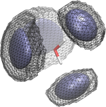
Figure 1: The filled areas represent the two-particle SDF computed for water at density $\rho_{0}=1.0$ g/cm³ (rendering of contour surface 0.17 of $\rho^{(2)}(\mathbf{R})/\rho_{0}$). The grids enclose the Bader domains, namely the volumes which are associated to the four highest maxima of the two-particle SDF obtained by the application of Bader analysis.

If we restrict ourselves to the four highest maxima of $\rho^{(2)}(\mathbf{R})$ computed for water, Bader analysis identifies the domains $\left\{\Delta_{i}\right\}_{i=1,4}$ that are represented by the volumes enclosed by the grids in Fig. 1. The filled areas are shown for reference and represent the function $\rho^{(2)}(\mathbf{R})$. For each domain, the probability of finding one, and only one, particle $P^{(1)}(\Delta_{i})$ is calculated from Eq. (7) and then maximized, by following the procedure illustrated above. The final domain is the MPD available to each particle surrounding the central water molecule.

The applications of the LSM are illustrated below. Before doing that, we find useful to stress two points.
(i) The results of our analysis do not depend on the initial set chosen. To that end, let us look at the result of the optimization performed using two different initial conditions for maxima of equivalent physical meaning. The first type of initial condition is a Bader domain (green areas in Fig. 2, left). The second, for different but equivalent maxima, is a sphere, approximately centered at the positions of the maxima of the SDF (blue areas in Fig. 2, left). Fig. 2 (right) shows that the shape of the MPDs is independent of the initial conditions.

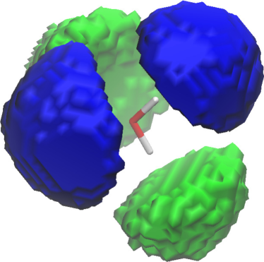
Figure 2: Left: different initial conditions for two sets of equivalent domains around a water molecule. Two domains are located in the region of the first solvation shell corresponding to the two oxygen atoms accepting the hydrogen bond; two domains appear in the region in the first solvation shell occupied by the two water molecules donating the hydrogen bonds. The green areas are Bader domains, whereas the blue areas are spheres with centers located at the positions of the maxima of the two-particle SDF. Right: the domains located at equivalent positions are identical after optimization.

(ii) When Bader analysis is applied in order to identify the initial domains, the space around the central particle (water molecule in our case) is partitioned as far as the two-particle SDF shows well defined local maxima. When the liquid approaches a random distribution Bader analysis becomes inefficient. In the case of water at density $\rho_{0}=1.0$ g/cm³ and $\rho=1.23$ g/cm³ presented in two following sections, we are able to identify and analyze domains up to within the third solvation shell ($6-8$ Å).

An additional point that is worth discussing here is the statistics. In order to increase the accuracy of our calculations in the case of pure water (Sections V.1 and V.2), we observe that all molecules are identical. Therefore, each molecule can be used as the central one, with respect to which the one-particle occupancy probability is calculated. This procedure is employed to overcome problems related to a short trajectory simulation. This same operation is, however, not possible in the case of sodium (Section V.3), because only one ion is present in the simulation box. In this case, since the problem has spherical symmetry, we increase the statistics by averaging over different orientations of the reference system centered on the ion.

V.1 Liquid water at $\rho_{0}=1.0$ g/cm³

The MD trajectory of 150 ps for liquid water at room temperature is generated by employing the TIP4P Jorgensen et al. (1983) model. The system is composed of 4096 molecules in a cubic box with side length 49.7 Å. Periodic boundary conditions are used throughout.

The 3D two-particle SDF has been calculated from the MD trajectory and, from the application of Bader analysis, the space around a central water molecule is partitioned in 15 regions within a distance of about 8 Å from the central oxygen atom. The resulting 15 MPDs give information on the structure of water up to within the third solvation shell, as we will now show.

Results will be presented by first looking at the MPDs in comparison to Bader domains. A 3D-map of the distribution of oxygen atoms surrounding the central water molecule is obtained. Each MPD is, on average, occupied by a single oxygen, thus such 3D-map has a very clear physical interpretation, pinpointing the locations of the oxygen atoms around a given water molecule. After this preliminary, more qualitative, presentation of the results, a few analysis tool will be introduced: we will classify the MPDs according to the corresponding value of the one-particle occupancy probability, according to their distance from the central oxygen atom and according to their volumes. These properties will be used to rationalize the differences between water at $\rho_{0}=1.0$ g/cm³ and at higher density, $\rho=1.23$ g/cm³, presented in the following section. Finally, the results shown here will be compared to more standard analysis tools, like RDFs, angular distributions and hydrogen bond structure.

V.1.1 Qualitative analysis of the MPDs in water

Figs. 3, 4 and 5 compare the results from Bader partitioning the space around a water molecule from the MPD analysis. In all figures, Bader domains are indicated as grids, while the MPDs are the filled regions.

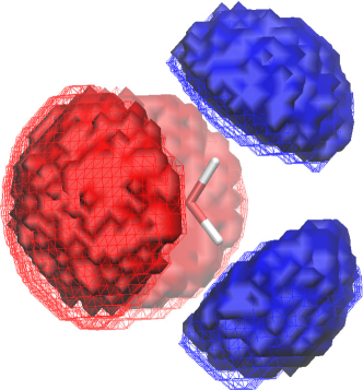
Figure 3: Case of water at $\rho_{0}=1.0$ g/cm³. MPDs (filled areas) labeled 1, 2 (blue) and 3, 4 (red) around the central water molecule. The initial Bader domains are also shown as grids.

The four MPDs in Fig. 3 clearly identify the regions occupied by the four water molecules hydrogen-bonded (H-bonded) to the central molecule, arranged according to the typical tetrahedral structure of the first solvation shell of water.

Fig. 4 shows the domains 5 to 10: domains 5 to 8 (left) are arranged on both sides of the plane defined by the central molecule in front of the hydrogen atoms and are symmetric with respect to this plane; domains 9 and 10 (right) are located in front of the hydrogen atoms of the central molecule and, after the optimization, are similar to domains 5 to 8.

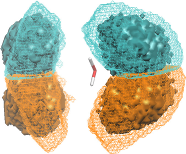
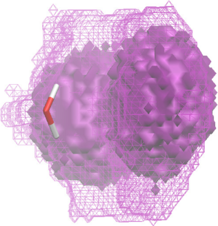
Figure 4: Case of water at $\rho_{0}=1.0$ g/cm³. Left: MPDs labeled 5, 6 (cyan) and 7, 8 (orange). Right: MPDs labeled 9, 10 (violet). The MPDs are compared to the initial Bader domains, represented as grids.

Domains 11 and 12 are shown in Fig. 5 (left) and, as will be proven below, they only partially occupy the first solvation shell, but they are mainly found in the second solvation shell, similarly to the domains 5 to 10. The MPDs 5 to 12 are interstitial domains, as they are located in correspondence of the empty spaces between the MPDs 1 to 4.

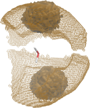
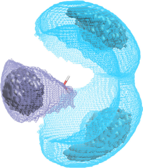
Figure 5: Case of water at $\rho_{0}=1.0$ g/cm³. Left: MPDs labeled 11, 12 (ochre areas). Right: MPDs labeled 13 (light-purple) and 14, 15 (turquoise). As in the previous figures, the initial Bader domains are shown for reference. We underline here that both pairs of domains 11, 12 and 14, 15 (Bader and MPDs) are completely symmetric with respect to the plane of the molecule and to its perpendicular plane.

The MPD labeled 13 (light-purple) in Fig. 5 (right) is also located in the second solvation shell, while further from the central molecule, the MPDs labeled 14, 15 (turquoise) are found as shown in Fig. 5 (right).

V.1.2 Some tools for a quantitative analysis

The MPDs around the central water molecule can be classified according to the value of the probability $P^{(1)}(\Delta)$ in each domain, as shown in table 1.

Label	$\left\langle N\right\rangle_{\textrm{before}}$	$\left\langle N\right\rangle_{\textrm{after}}$	Volume (Å3)	Distance (Å)	$P^{(1)}(\Delta^{*})$
1, 2	1.2	1.1	14.9	2.8	0.9,0.91
3, 4	1.6	1.0	15.2	2.6	0.78
5 - 8	2.0	1.2	15.8	4.2	0.63
9, 10	1.8	1.1	15.9	4.3	0.63
11, 12	5.9	1.1	15.8	4.4	0.63
13	3.0	1.8(a)	17.2	4.5	0.37(a)
14, 15	4.0	0.6(a)	21.1	6.5	0.61(a)

Table 1: List of the MPDs (first column), average number of particles in each volume before (Bader analysis, second column) or after the optimization (third column), volumes of the MPDs (fourth column), distances of the centers of mass of the MPDs from the central oxygen atom (fifth column) and the one-particle occupancy probability (sixth column). In the same line of the first column we have put equivalent domains. ^(a)The values of $\left\langle N\right\rangle_{\textrm{after}}$ and $P^{(1)}(\Delta^{*})$ for the volumes 13 and 14, 15 are in italic to indicate that the optimization procedure seems to be in these cases less efficient than for the other domains: in the first case, the optimization appears not able to split the domains in two parts; in the second case, the density of the liquid is probably too flat, thus preventing from an efficient analysis.

The domains labeled 1, 2 are associated to a higher probability than the domains 3, 4. This difference can be explained as follows. Domains 1, 2 enclose the oxygen atoms of the two water molecules H-bonded to the hydrogen atoms of the central water molecule, namely HO$\cdots$H_central. Domains 3, 4 enclose the oxygen atoms of the molecules that are H-bonded to the central one as OH$\cdots$O_central. Therefore, in the latter case, the oxygen atoms are not directly bonded to the central molecule, thus resulting more mobile.

The probability of finding only one water molecule inside domains 5 to 12 is further reduced compared to the previous case. It follows that a high probability is an indication of a strong bond, like a H-bond, while a lower probability suggests the absence of a strong interaction, as in the case of the oxygen atoms in the interstitial domains.

Table 1 shows also the volumes associated to each MPDs and their distance from the oxygen atom of the central water molecule, expressed in terms of the distance of their centers of mass. In particular, we notice the clear identification of three groups of domains, whose distances from the central molecule are below 3 Å, between 4 and 5 Å, above 6 Å. We will see below how this structure changes upon increasing the density. We also observe the increase of the volume of the domain itself as its distance from the central oxygen increases. The correlation to the central water molecule is reduced, then the surrounding molecules are more mobile and occupy larger volumes. Observations about the effect of the interactions on the volume of the MPDs are reported in Appendix C.

V.1.3 Comparison with standard analysis tools

Since the domains 1 to 4 enclose the oxygen atoms of the water molecules that are H-bonded to the central molecule, we can define an estimate of the number $n_{\mathrm{HB}}$ of hydrogen bonds (HBs) formed by a water molecule. Indeed the domains indicate only the positions of the oxygen atoms, and therefore, domains 3 and 4 cannot, strictly speaking, be used to estimate the presence of HBs. This is because in those regions the hydrogen atoms (not the oxygens) form HBs with the central water molecule. However, the H-bonded hydrogens are close to the oxygens occupying the domains 3 and 4. If we take a high one-particle occupancy probability as an indication of the presence of a HB, then its value can qualitatively measure the fraction of HBs present. Taking that the four closest domains do not superpose (a hypothesis almost always satisfied, but certainly an approximation Luzar and Chandler (1996)), we can sum up their probabilities to have an indication of how many HBs are formed around a water molecule:

$$n_{\mathrm{HB}}=\sum_{i=1}^{4}P^{(1)}(\Delta_{i}).$$ (14)

In a transient configuration, when one hydrogen bond is broken before another is formed, it is plausible to assume that the domain is occupied by a number of water molecules different from one. According to Eq. (14), we find that the average number of HBs formed by a water molecule is $n_{\mathrm{HB}}=3.37$, in agreement Luzar and Chandler (1996); Wernet et al. (2004) with the values reported in the literature of $3.3-3.6$.

In the context of the MPDs, solvation shells can be defined by calculating the oxygen-oxygen RDF resolved in each optimized domain. In Fig. 6 we show the RDFs computed within the MPDs (lower panel) and compared to the total RDF (upper panel). The $x$-axis has been divided in three regions, each representing a solvation shell around the central water molecule. The extent of the first solvation shell is up to about 3.5 Å. The MPDs labeled from 5 to 12 (corresponding to the blue and magenta lines in Fig. 6) only partially occupy the cavities between the domains 1 to 4 of the first solvation shell, but they extend to the second solvation shell.

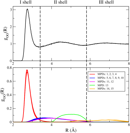
Figure 6: Oxygen-oxygen RDFs (colored lines) computed within the MPDs, compared to the total RDF of water at density $\rho_{0}$ (black line). Dashed vertical lines are used to show that space partitioning in terms of solvation shells (from the minima of the oxygen-oxygen RDF) or MPDs brings to a similar result (for instance the boundary between the second and third solvation shell is not exactly placed at the minimum of the total RDF).

The coordination number in the first solvation shell is 5.1, if computed as the integral of the total RDF up to 3.5 Å, and 4.5, if computed as the sum of the integrals of the partial RDFs. An extra-particle Sciortino et al. (1990) appears in the first solvation shell, which does not occupy one of the four domains of the tetrahedron, but it is delocalized in the interstitial domains 5 to 12. Particularly interesting is the distribution of particles in these interstitial domains since the partial RDFs, although very flat, show peaks at about 3.5 Å. Similar maxima have been already observed by Svishchev and Kusalik Svishchev and Kusalik (1993) from calculation of RDFs resolved in angle. This feature of the RDFs suggests the presence of water molecules in non-tetrahedral directions but still penetrating the first solvation shell.

V.2 Liquid water at $\rho=1.23$ g/cm³

The MD trajectory of 150 ps for liquid water at room temperature is generated by employing the TIP4P Jorgensen et al. (1983) model. The system is composed of 4096 molecules in a cubic box with side length 46.3 Å.

Bader analysis is applied to the two-particle SDF computed for liquid water at the density $\rho=1.23$ g/cm³ and 11 domains are identified, in contrast to the previous case where 15 domains were defined by Bader analysis. The shapes and positions of the initial domains are shown in Fig. 7 (left) along with the MPDs (right). We will present here the results from the MPD analysis in comparison to the observations reported in the previous section.

V.2.1 Comparison with water at $\rho_{0}$ based on the MPD analysis

The first solvation shell is unaffected Saitta and Datchi (2003); Yan et al. (2007) by the increase of density. The remaining domains are arranged closer to the central molecule and they are more localized in space.

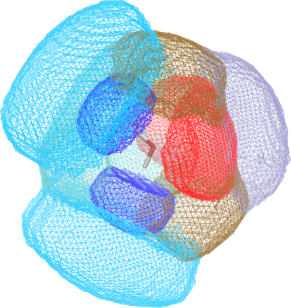
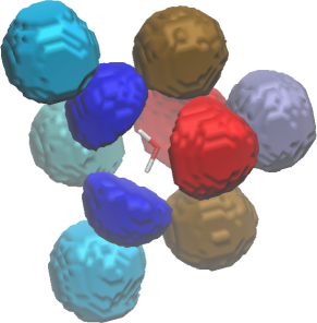
Figure 7: Case of water at $\rho=1.23$ g/cm³. Left: Bader domains for water at $\rho=1.23$ g/cm³. Only one domain of those labeled 5 and 6 (one of these two domains is shown as the black filled area in Fig. 8) is shown, in order to make the central water molecule visible. Right: MPDs.

Since the water molecules are more “packed” at higher density and the maxima of the $\rho^{(2)}(\mathbf{R})$ are less sharp, Bader domains 5 to 10 from Fig. 4 merged into two domains, as shown in Fig. 8.

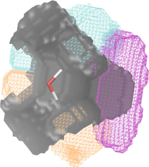
Figure 8: Comparison of Bader domains for water at density $\rho_{0}=1.0$ g/cm³ (color grids) and at density $\rho=1.23$ g/cm³ (black filled areas).

The MPDs can be grouped according to the corresponding final probability of enclosing only one particle, shown in table 2. If we use again Eq. (14) to estimate the value of HBs per molecule, we find $n_{\mathrm{HB}}=3.41$. Apart from this aspect, the optimized domains in the first solvation shell are not very much affected by the change of density. This observation agrees Saitta and Datchi (2003); Yan et al. (2007); Soper and Ricci (2000); Jedlovszky et al. (2008); Strässle et al. (2006) with the literature, namely the MPDs analysis confirms that the first solvation shell is quite rigid under density increase.

Looking at the one-particle occupancy probability of the MPDs 5 to 11, listed in table 2, the optimization procedure seems to be more effective in this case of higher density. Also, the average number of particles found in each MPD is very close to one for all domains. This effect can be interpreted as a stabilization of the molecules in the second solvation shell due to the packing imposed by the higher density.

Domain label	$\left\langle N\right\rangle_{\textrm{before}}$	$\left\langle N\right\rangle_{\textrm{after}}$	Volume (Å3)	Distance (Å)	$P^{(1)}(\Delta^{*})$
1, 2	0.7	0.9	12.6	2.7	0.93
3, 4	1.7	1.0	12.0	2.8	0.78
5, 6	5.1	1.3	14.5	3.7	0.74
7, 8	2.7	1.3	15.0	4.0	0.72
9	2.4	1.0	15.8	4.7	0.68
10, 11	5.0	0.9	16.1	5.6	0.70

Table 2: List of the MPDs (first column), average number of particles in each volume before (Bader analysis, second column) or after the optimization (third column), their volumes (fourth column), distances of their centers of mass from the central oxygen atom (fifth column) and the one-particle occupancy probability (sixth column). In the same line of the first column we have put equivalent domains.

Comparing the distances of the MPDs from the central molecule at the two densities, $\rho_{0}$ and $\rho$, we observe a major difference in the behavior of domains 5 and 6, found at a distance of 3.7 Å as shown in table 2, from the behavior of the set of domains at a distance between 4 and 5 Å reported in table 1. This result is extremely interesting, as it seems that we have been able to identify, in terms of the MPDs, the location of the interstitial oxygen atoms that are mainly affected by the increase of the density. As proven in Fig. 9, not all the interstitial domains are strongly affected by the change of density (see the difference between the blue and the magenta curves). The pronounced peak (blue line in the figure) in the partial RDFs corresponding to the MPDs 5 and 6 at around 3.3 Å contributes to the shoulder in the total oxygen-oxygen RDF at the same distance (highlighted in the figure by the circle). In the previous analysis we showed that all domains in these regions, namely those labeled 5 to 12, have similar partial RDFs (blue and magenta lines in Fig. 6). Instead we observe here that the partial RDFs calculated inside the domains 5, 6 show a more pronounced peak than the domains 7, 8. In general, we can observe that the MPDs 5 to 8 enclose the four molecules Saitta and Datchi (2003) that in non-tetrahedral directions Jedlovszky et al. (2008); Svishchev and Kusalik (1993) mainly contribute to modifications of the second solvation shell at increasing density. The hypothesis Saitta and Datchi (2003) that, as the density increases, the second solvation shell does not continuously collapse on the first shell but interstitial molecules, that are not H-bonded to the first shell molecules, get closer to the central water is consistent with our results.

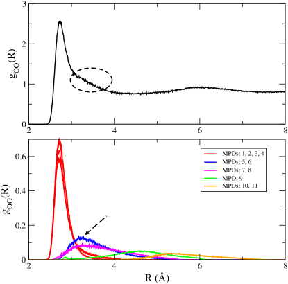
Figure 9: Oxygen-oxygen RDFs computed within each MPD, compared to the total RDF of water at density 1.23 g/cm³. In the upper panel, the shoulder in the highlighted region is produced by the curves in the lower panel which are indicated by the arrow.

V.3 $\bf{Na^{+}}$ in water

The MD trajectory of 110 ps for a sodium ion in liquid water, at room temperature, is generated by employing the TIP4P Jorgensen et al. (1983) model for water. The system is composed of 1024 molecules in a cubic box with side length 31.5 Å.

The sodium-oxygen SDF is spherically symmetric and it does not contain more information than the sodium-oxygen RDF, therefore the MPDs will have the same spherical distribution around the central ion. The position and shape of the initial domains can be chosen totally arbitrarily, since Bader analysis is not efficient in this situation, where the local maxima of the two-particle SDF cannot be properly located (maxima of the density are distributed on a sphere, they are not isolated points in 3D space). Also, if the initial domains are chosen within a distance of less than about 2.2 Å, where the RDF (see Fig. 11) is very small, the optimization procedure is not efficient and the MPDs cannot be identified. This problem is related to the fact that in empty regions, where the probability of finding one particle vanishes, a small variation of the region itself does not change this probability, thus fulfilling the optimization condition $|P^{(1)}(\Delta_{\tau})-P^{(1)}(\Delta)|\leq\delta$ without an effective modification of the domain. Here, we have considered only domains $\Delta$ that are enclosed in the region of non-zero probability density. We then choose, as initial domains, spheres of different radii, randomly located around the central ion and at distances between 2.5 Å and 4.5 Å from it.

As in the previous applications, we will first show the MPDs and then we will introduce some analysis tools to determine the properties of the MPDs.

V.3.1 Analysis of the MPDs

The optimization procedure identifies two sets of MPDs, associated to the first and second solvation shells of water around the central sodium ion. They are shown in Fig. 10 as blue and red grid volumes, with distances from the central ion of 2.3 and 4.4 Å, respectively. These values are listed in table 3, along with the other properties associated to the two MPDs.

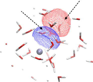
Figure 10: Case of sodium diluted in water. MPDs in the first and second solvation shells of Na⁺. From a snapshot of the trajectory, some water molecules in the vicinity of the central ion are also shown. We see that each domain is occupied by only one molecule (indicated by the arrows).

Shell	Volume (Å3)	Distance (Å)	$\Omega$ (deg2)	$n_{\Omega}$	$P^{(1)}(\Delta^{*})$
I	12.0	2.3	135.6	5.3 (5.9)	0.78
II	16.2	4.4	39.9	18.1 (19.3)	0.62

Table 3: List of properties of the MPDs calculated for Na⁺ in water. In the first column we list the position of the domain, in one of the two solvation shells around the sodium ion, in the second we calculate the volumes occupied by the domain, in the third column we report the distance of the center of mass of the domain from the central ion, in the fourth column we show the solid angle occupied by the domain and in the fifth column, the coordination number associated to it. In parenthesis, we compare the value of the coordination number determined by integrating the RDF up to $R=$3.3,5.6 Å. In the sixth column the values of the one-particle occupancy probability are given.

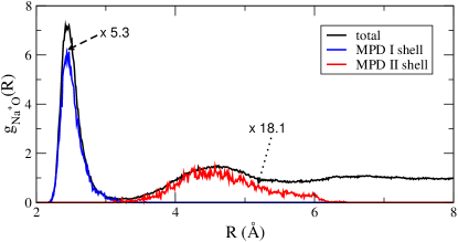
Figure 11: Total and partial (calculation restricted to each given domain) ion-oxygen RDF. The blue and red curves are determined by calculating the RDF in the domains shown in Fig. 10 and by multiplying it by the corresponding $n_{\Omega}$ (from table 3).

The coordination number $n_{\Omega}$ in the two shells is determined as the ratio of the solid angle occupied by the domain $\Omega$ and the total solid angle, whose values are shown in table 3. In particular, the coordination numbers $n_{\Omega}$ are in very good agreement with those determined by integrating the RDF up to the distances 3.3 and 5.6 Å, for the first and second solvation shell, respectively. As also observed in the case of water, slightly smaller values are determined by our analysis, if compared to the integral of the RDF. The total RDF can be reconstructed by determining its value inside the MPDs. The comparison between the total RDF and the partial ones (in each domain) is shown in Fig. 11. The curves calculated in the two domains are multiplied by the corresponding $n_{\Omega}$ in order to obtain the contribution from the whole shell.

VI Conclusions

We extended the study of the structure of a liquid system by the identification of MPDs, borrowing the idea from what is now routinely done in electronic structure analysis, and we developed a first application to few case studies. We derived the formalism necessary to define the probability of finding one and only one particle in a certain region of space $\Delta$ and we developed an algorithm for the optimization of this region under the request that the probability is maximized. The geometric optimization is formulated in terms of shape derivatives, thus allowing to use the LSM to solve the optimization problem.

The case study obtained the features of the MPDs for water at different densities and for a solvated sodium ion in water. A qualitative analysis of the domains in water has allowed us to describe the modification of the second solvation shell by increasing pressure. More quantitative observations have also illustrated the presence of water molecules in the interstitial spaces of the first solvation shell, that are not H-bonded to the central molecule. These molecules contribute to the modification of the second solvation shell of water at increasing density. Looking at the RDFs restricted to the MPDs, we have been able to indirectly achieve a 3D resolution that is totally lacking in the (standard) full oxygen-oxygen RDF, since we know exactly the spatial organization of the MPDs. Therefore, this result proves that this new approach adds to standard techniques, providing structural 3D information on liquids. In the case of a sodium ion in water, we reconstructed the sodium-oxygen RDF from the partial contributions evaluated inside the optimized domains and we determined the coordination numbers associated to these domains. We used a criterion to identify the solvation shells, based on the identification of regions where the partial RDFs, calculated within the MPDs, are close to zero, rather than on the identification of the minima of the total RDF. Notice that, even though we started the research for the MPDs around the sodium ion from the information obtained from the RDFs (but only as input in the analysis, the distance from the central ion of the maxima of the sodium-oxygen RDF), we have extracted the full 3D shape of the domains containing the oxygen atoms around the sodium ion. In this case, in fact the sodium-oxygen SDF cannot provide this information, since the problem has spherical symmetry.

We investigated the properties of the MPDs that are determined from the maximization of the one-particle occupancy probability. Along similar lines one could analyze probabilities associated to more than one particle or focus on other atoms (hydrogens, for instance). This could be used to give a many-body definition of solvation shells.

The proposed method results to be an efficient tool to complement the standard analysis techniques used in the study of the structure of a liquid system and to give the 3D image of the organization of the space around a given molecule, atom or ion. To conclude, let us say that, despite the somehow elaborate mathematical construction presented in the paper, the physical interpretation of the MPD approach is simple. It allows to identify at 3D level the statistical meaning of the positions of particles surrounding a given central molecule or ion. To do that, it looks at new and different (from those in standard use) probabilities, allowing to better isolate the 3D statistical arrangement of the observed particles.

Appendix A Probability density

We have illustrated how to use the MPDs to investigate the local structure of a liquid around a given center. In the examples discussed in the paper, the center was chosen as a water molecule, in the case of liquid water, and as the sodium ion, in the case where we analyze the structure of the water solvation shells around this ion. Therefore, the probability density $\rho(\mathbf{R}^{N})$ introduced in Eq. (1) has to be identified as the conditional probability density of the configuration $\mathbf{R}^{N}$ of the $N$ oxygen atoms, given a certain configuration $\{\mathbf{R}_{0},\mathbf{R}^{\mathrm{H}_{1}}_{0},\mathbf{R}^{\mathrm{H}_{2}}_{0}\}$ of the central water molecule,

$$\rho(\mathbf{R}^{N})=\rho\left(\mathbf{R}^{N}\left|\right.\mathbf{R}_{0},\mathbf{R}^{\mathrm{H}_{1}}_{0},\mathbf{R}^{\mathrm{H}_{2}}_{0}\right),$$ (15)

or of the central sodium ion $\{\mathbf{R}^{\mathrm{Na}^{+}}_{0}\}$,

$$\rho(\mathbf{R}^{N})=\rho\left(\mathbf{R}^{N}\left|\right.\mathbf{R}^{\mathrm{Na}^{+}}_{0}\right).$$ (16)

We explicitly discuss below only the case of water, while the expressions for sodium in water are obtained by replacing $\{\mathbf{R}^{\mathrm{Na}^{+}}_{0}\}$ to $\{\mathbf{R}_{0},\mathbf{R}^{\mathrm{H}_{1}}_{0},\mathbf{R}^{\mathrm{H}_{2}}_{0}\}$.

Here we label with “0” the positions of the oxygen atom and the two hydrogen atoms of the central molecule. To be more explicit on the relation between the density in Eq. (15) and the standard configurational canonical density $\rho^{can}(\mathbf{R}_{0},\mathbf{R}^{N},\mathbf{R}^{\mathrm{H}_{1}}_{0},\mathbf{R}^{\mathrm{H}_{2}}_{0},{\mathbf{R}^{\mathrm{H}_{1}}}^{N},{\mathbf{R}^{\mathrm{H}_{2}}}^{N})$, that is a function of all atomic positions, i.e. oxygens and hydrogens, we give the following expression of $\rho(\mathbf{R}^{N})$,

$$\rho(\mathbf{R}^{N})= \int d{\mathbf{R}^{\mathrm{H}_{1}}}^{N}\,d{\mathbf{R}^{\mathrm{H}_{2}}}^{N}\,\frac{\rho^{can}\left(\mathbf{R}_{0},\mathbf{R}^{N},\mathbf{R}^{\mathrm{H}_{1}}_{0},\mathbf{R}^{\mathrm{H}_{2}}_{0},{\mathbf{R}^{\mathrm{H}_{1}}}^{N}_{1},{\mathbf{R}^{\mathrm{H}_{2}}}^{N}\right)}{P_{m}\left(\mathbf{R}_{0},\mathbf{R}^{\mathrm{H}_{1}}_{0},\mathbf{R}^{\mathrm{H}_{2}}_{0}\right)}.$$ (17)

Since $\rho(\mathbf{R}^{N})$ is a conditional probability density, the denominator represents the marginal probability of finding the central molecule in the configuration $\{\mathbf{R}_{0},\mathbf{R}^{\mathrm{H}_{1}}_{0},\mathbf{R}^{\mathrm{H}_{2}}_{0}\}$, namely

$$P_{m}\left(\mathbf{R}_{0},\mathbf{R}^{\mathrm{H}_{1}}_{0},\mathbf{R}^{\mathrm{H}_{2}}_{0}\right)=\int d\mathbf{R}^{N}\,d{\mathbf{R}^{\mathrm{H}_{1}}}^{N}\,d{\mathbf{R}^{\mathrm{H}_{2}}}^{N}\,\rho^{can}\left(\mathbf{R}_{0},\mathbf{R}^{N},\mathbf{R}^{\mathrm{H}_{1}}_{0},\mathbf{R}^{\mathrm{H}_{2}}_{0},{\mathbf{R}^{\mathrm{H}_{1}}}^{N},{\mathbf{R}^{\mathrm{H}_{2}}}^{N}\right).$$ (18)

Appendix B The level set method

We present here in detail the LSM, defining the shape derivative of $P^{(1)}(\Delta)$ and introducing the level set function.

B.1 Shape derivative

$P^{(1)}(\Delta)$ belongs to a specific class of what is normally called a set function. We now introduce few analysis tools used when treating in general set functions.

The shape derivative of a set function of the form

$$F(\Delta)=\int_{\Delta}d\mathbf{R}\,f(\mathbf{R})$$ (19)

is defined as the variation with respect to the integration domain $\Delta$. In other words $F(\Delta)$ can be written in terms of a “density”, $f(\mathbf{R})$, and, in the following section, we give the explicit definition of the $f(\mathbf{R})$, interesting us, from Eq. (4).

If the deformation law of $\Delta$ is given as

$$\Delta\rightarrow\Delta_{\tau}=\left\{\mathbf{R}_{\tau}=\mathbf{R}+\mathbf{v}(\mathbf{R})d\tau\,|\,\mathbf{R}\in\partial\Delta\right\}$$ (20)

where $d\tau$ is a fictitious time step and $\mathbf{v}(\mathbf{R})$ is a velocity field (to be specified below), the time derivative of $F(\Delta)$ can be calculated according to

$$\frac{dF(\Delta)}{d\tau}=\lim_{d\tau\rightarrow 0}\frac{1}{d\tau}\left[\int_{\Delta_{\tau}}d\mathbf{R}_{\tau}\,f(\mathbf{R}_{\tau})-\int_{\Delta}d\mathbf{R}\,f(\mathbf{R})\right].$$ (21)

Performing, in the first term in square brackets, the change of variable

$$\mathbf{R}_{\tau}=\mathbf{R}+\mathbf{v}(\mathbf{R})d\tau,\quad d\mathbf{R}_{\tau}=d\mathbf{R}\left(1+\nabla\cdot\mathbf{v}(\mathbf{R})d\tau+\mathcal{O}(d\tau^{2})\right)$$ (22)

and expanding, for small time increment $d\tau$, $f(\mathbf{R}_{\tau})$ around $\mathbf{R}$

$$f(\mathbf{R}_{\tau})=f(\mathbf{R})+\mathbf{v}(\mathbf{R})\cdot\nabla f(\mathbf{R})d\tau,$$ (23)

Eq. (21) becomes

$$\frac{dF(\Delta)}{d\tau} = \int_{\Delta}d\mathbf{R}\,\nabla\cdot\left(\mathbf{v}(\mathbf{R})f(\mathbf{R})\right)$$ (24)

$$= \int_{\partial\Delta}ds\,\mathbf{n}(\mathbf{R})\cdot\mathbf{v}(\mathbf{R})f(\mathbf{R})\equiv\mathcal{D}_{S}F(\Delta)$$ (25)

where the divergence theorem has been used to derive Eq. (25) from Eq. (24). In the last line $ds$ is the surface element of the boundary $\partial\Delta$ of $\Delta$ and $\mathbf{n}(\mathbf{R})$ is the unit vector normal to the surface at $\mathbf{R}$. Eq. (25) defines the shape derivative, indicated by the symbol $\mathcal{D}_{S}$, of $F(\Delta)$ and expresses the variation of $F(\Delta)$ with respect to the variation of $\Delta$. The change in the domain $\Delta$ is expressed in terms of a global deformation of the boundary $\partial\Delta$, which, in turn, is determined by the velocity field $\mathbf{v}(\mathbf{R})$. For our purpose, that is the maximization of $F(\Delta)$, we can choose the field $\mathbf{v}(\mathbf{R})$ such that $\mathcal{D}_{S}F(\Delta)\geq 0$ and follow the evolution of such a field up to find the final $\mathcal{D}_{S}F(\Delta)=0$. The condition $\mathcal{D}_{S}F(\Delta)\geq 0$ is automatically satisfied if we choose the velocity field as

$$\mathbf{v}(\mathbf{R})=\mathbf{n}(\mathbf{R})f(\mathbf{R}).$$ (26)

B.2 Shape derivative for the MPDs

The comparison between Eqs. (1) and (19) shows that when we express the probability $P^{(1)}(\Delta)$ in terms of a density function similar to $f(\mathbf{R})$, such density depends on $\Delta_{c}$, i.e. on $\Delta$. Therefore, when calculating the variations of $F(\Delta)$ from Eq. (19) with respect to $\Delta$, we need to include also variations of $f(\mathbf{R})$ with respect to $\Delta_{c}$, i.e. $\Delta$. In our case, then, the transformation in Eq. (22), restricting ourselves to the case $\mathbf{v}_{j}(\mathbf{R})=\mathbf{v}(\mathbf{R}_{j})$, becomes

$$\mathbf{R}_{j,\tau} =\mathbf{R}_{j}+\mathbf{v}(\mathbf{R}_{j})d\tau\quad\mbox{with }j=1,\ldots,N$$ (27)

and the volume elements are

$$d\mathbf{R}_{j,\tau} =d\mathbf{R}_{j}\left(1+\nabla_{\mathbf{R}_{j}}\cdot\mathbf{v}(\mathbf{R}_{j})d\tau\right).$$ (28)

The time derivative of the probability $P^{(1)}(\Delta)$ under the variation $\Delta\rightarrow\Delta_{\tau}$ is

$$\frac{dP^{(1)}(\Delta)}{d\tau} =$$

$$\lim_{d\tau\rightarrow 0} \frac{1}{d\tau}\sum_{i=1}^{N}\Big{[}\int_{\Delta_{\tau}}d\mathbf{R}_{i,\tau}\left(\prod_{l\neq i}^{N}\int_{\Delta_{c},\tau}d\mathbf{R}_{l,\tau}\right)\rho(\mathbf{R}_{\tau}^{N})-\int_{\Delta}d\mathbf{R}_{i}\left(\prod_{l\neq i}^{N}\int_{\Delta_{c}}d\mathbf{R}_{l}\right)\rho(\mathbf{R}^{N})\Big{]}$$ (29)

where $\Delta_{c,\tau}$ is the complementary volume to $\Delta_{\tau}$, $d\mathbf{R}_{\tau}^{N-1}=d\mathbf{R}_{2,\tau}\ldots d\mathbf{R}_{N,\tau}$ (similarly for $d\mathbf{R}^{N-1}$) and $\mathbf{R}^{N}_{\tau}=\mathbf{R}_{1,\tau},\ldots,\mathbf{R}_{2,\tau}$. Using Eq. (28) and the expansion of the density $\rho(\mathbf{R}_{\tau}^{N})$ up to linear order (see Eq. (23)) in the displacement from $\mathbf{R}^{N}$,

$$\rho(\mathbf{R}_{\tau}^{N})=\rho(\mathbf{R}^{N})+\sum_{j=1}^{N}\left[\nabla_{\mathbf{R}_{j}}\rho(\mathbf{R}^{N})\right]\cdot\mathbf{v}(\mathbf{R}_{j})d\tau,$$ (30)

the shape derivative of $P^{(1)}(\Delta)$ becomes

$$\frac{dP^{(1)}(\Delta)}{d\tau}=\sum_{i=1}^{N}\int_{\Delta} d\mathbf{R}_{i}\left(\prod_{l\neq i}^{N}\int_{\Delta_{c}}d\mathbf{R}_{l}\right)\Bigg{[}\nabla_{\mathbf{R}_{i}}\cdot\Big{(}\rho(\mathbf{R}^{N})\mathbf{v}(\mathbf{R}_{i})\Big{)}+\sum_{j\neq i}^{N}\nabla_{\mathbf{R}_{j}}\cdot\Big{(}\rho(\mathbf{R}^{N})\mathbf{v}(\mathbf{R}_{j})\Big{)}\Bigg{]}.$$ (31)

The first term on the right-hand-side can be treated exactly as we have done in Eq. (24), leading to

$$\int_{\Delta}d\mathbf{R}_{i}\left(\prod_{l\neq i}^{N}\int_{\Delta_{c}}d\mathbf{R}_{l}\right)\nabla_{\mathbf{R}_{i}}\cdot\Big{(}\rho(\mathbf{R}^{N})\mathbf{v}(\mathbf{R}_{i})\Big{)}=\int_{\partial\Delta}ds_{i}\,\mathbf{n}(\mathbf{R}_{i})\cdot\mathbf{v}(\mathbf{R}_{i})\left(\prod_{l\neq i}^{N}\int_{\Delta_{c}}d\mathbf{R}_{l}\right)\rho(\mathbf{R}^{N})$$

$$=\int_{\partial\Delta}ds\,\mathbf{n}(\mathbf{R})\cdot\mathbf{v}(\mathbf{R})\int d\mathbf{R}_{i}\,\delta\left(\mathbf{R}_{i}-\mathbf{R}\right)\left(\prod_{l\neq i}^{N}\int_{\Delta_{c}}d\mathbf{R}_{l}\right)\rho(\mathbf{R}^{N}).$$ (32)

The second line is obtained from the first by introducing a $\delta$-function in order to change the variable $\mathbf{R}_{i}$ to $\mathbf{R}$ in the surface integral. Notice now that the integral over the variable $\mathbf{R}_{i}$ is performed over the whole space.

The second term in Eq. (31) has still to be appropriately simplified. The $N-1$ integrals of the second term in square brackets are transformed, one by one, in $N-1$ surface integrals over $\partial\Delta_{c}$ with $\nabla_{\mathbf{R}_{j}}\cdot$ replaced by the normal vector to the surface, $\mathbf{n}_{c}(\mathbf{R}_{j})=-\mathbf{n}(\mathbf{R}_{j})$ (when the volume $\Delta$ changes in the direction indicated by $\mathbf{n}$, the volume $\Delta_{c}$ changes in the direction $-\mathbf{n}$, since the boundaries of $\Delta$ and $\Delta_{c}$ are the same, being them complementary volumes to each other). Therefore, we write explicitly each term of the sum over the index $j$ in Eq. (31)

$$\int_{\Delta}d\mathbf{R}_{i}\left(\prod_{l\neq i}^{N}\int_{\Delta_{c}}d\mathbf{R}_{l}\right) \sum_{j\neq i}^{N}\nabla_{\mathbf{R}_{j}}\cdot\Big{(}\rho(\mathbf{R}^{N})\mathbf{v}(\mathbf{R}_{j})\Big{)}=$$

$$\int_{\Delta}d\mathbf{R}_{i}\int_{\partial\Delta_{c}}ds_{1}\left(\prod_{l\neq i,1}\int_{\Delta_{c}}d\mathbf{R}_{l}\right)\mathbf{n}_{c}(\mathbf{R}_{1})\cdot\mathbf{v}(\mathbf{R}_{1})\rho(\mathbf{R}^{N})$$

$$+\int_{\Delta}d\mathbf{R}_{i}\int_{\partial\Delta_{c}}ds_{2}\left(\prod_{l\neq i,2}\int_{\Delta_{c}}d\mathbf{R}_{l}\right)\mathbf{n}_{c}(\mathbf{R}_{2})\cdot\mathbf{v}(\mathbf{R}_{2})\rho(\mathbf{R}^{N})+\ldots$$ (33)

obtaining

$$\int_{\Delta}d\mathbf{R}_{i}\left(\prod_{l\neq i}^{N}\int_{\Delta_{c}}d\mathbf{R}_{l}\right) \sum_{j\neq i}^{N}\nabla_{\mathbf{R}_{j}}\cdot\Big{(}\rho(\mathbf{R}^{N})\mathbf{v}(\mathbf{R}_{j})\Big{)}=$$

$$\int_{\Delta}d\mathbf{R}_{i}\sum_{j\neq i}^{N}\int_{\partial\Delta_{c}}ds_{j}\left(\prod_{l\neq i,j}\int_{\Delta_{c}}d\mathbf{R}_{l}\right)\mathbf{n}_{c}(\mathbf{R}_{j})\cdot\mathbf{v}(\mathbf{R}_{j})\rho(\mathbf{R}^{N}).$$ (34)

We introduce now a $\delta$-function, in order to make a change of variable $\mathbf{R}_{j}\rightarrow\mathbf{R}$ and to write the above integral in compact form, namely

$$\int_{\Delta}d\mathbf{R}_{i} \left(\prod_{l\neq i}^{N}\int_{\Delta_{c}}d\mathbf{R}_{l}\right)\sum_{j\neq i}^{N}\nabla_{\mathbf{R}_{j}}\cdot\Big{(}\rho(\mathbf{R}^{N})\mathbf{v}(\mathbf{R}_{j})\Big{)}=$$

$$\int_{\Delta}d\mathbf{R}_{i}\sum_{j\neq i}^{N}\int_{\partial\Delta_{c}}ds\,\mathbf{n}_{c}(\mathbf{R})\cdot\mathbf{v}(\mathbf{R})\int d\mathbf{R}_{j}\,\delta\left(\mathbf{R}_{j}-\mathbf{R}\right)\left(\prod_{l\neq i,j}\int_{\Delta_{c}}d\mathbf{R}_{l}\right)\rho(\mathbf{R}^{N})$$ (35)

$$=-\int_{\Delta}d\mathbf{R}_{i}\sum_{j\neq i}^{N}\int_{\partial\Delta}ds\,\mathbf{n}(\mathbf{R})\cdot\mathbf{v}(\mathbf{R})\int d\mathbf{R}_{j}\,\delta\left(\mathbf{R}_{j}-\mathbf{R}\right)\left(\prod_{l\neq i,j}\int_{\Delta_{c}}d\mathbf{R}_{l}\right)\rho(\mathbf{R}^{N}).$$ (36)

From Eq. (35) we have obtained Eq. (36) by replacing $\mathbf{n}_{c}$ with $-\mathbf{n}$ and by using the property that the boundary of $\Delta_{c}$ is the boundary of $\Delta$. As previously observed for Eq. (32), the integral over the variable $\mathbf{R}_{j}$ is performed over the whole space.

Combining the results in Eqs. (32) and (36), we derive the expression for the shape derivative of the one-particle occupancy probability as

$$\frac{dP^{(1)}(\Delta)}{d\tau}=\int_{\partial\Delta}ds\,\mathbf{n}(\mathbf{R})\cdot\mathbf{v}(\mathbf{R})\,\left\{\sum_{i=1}^{N}\Bigg{[}\int d\mathbf{R}_{i}\,\delta\left(\mathbf{R}_{i}-\mathbf{R}\right)\left(\prod_{l\neq i}^{N}\int_{\Delta_{c}}d\mathbf{R}_{l}\right)\right.$$ (37)

$$\left.-\int_{\Delta}d\mathbf{R}_{i}\sum_{j\neq i}^{N}\int d\mathbf{R}_{j}\,\delta\left(\mathbf{R}_{j}-\mathbf{R}\right)\left(\prod_{l\neq i,j}\int_{\Delta_{c}}d\mathbf{R}_{l}\right)\Bigg{]}\rho(\mathbf{R}^{N})\right\}.$$ (38)

The characteristic functions $\Upsilon_{\Delta}(\mathbf{R}_{j})$ and $\Upsilon_{\Delta_{c}}(\mathbf{R}_{j})=1-\Upsilon_{\Delta}(\mathbf{R}_{j})$ $\forall j$ are used in order to extend the integrals over $\Delta$ and $\Delta_{c}$ to the whole space. We then obtain

$$\frac{dP^{(1)}(\Delta)}{d\tau}=\int_{\partial\Delta}ds\,\mathbf{n}(\mathbf{R})\cdot\mathbf{v}(\mathbf{R})f_{\Delta}(\mathbf{R})$$ (39)

with

$$f_{\Delta}(\mathbf{R})= \left\langle\sum_{i=1}^{N}\Bigg{[}\delta\left(\mathbf{R}_{i}-\mathbf{R}\right)\prod_{l\neq i}^{N}\left(1-\Upsilon_{\Delta}(\mathbf{R}_{l})\right)-\sum_{j\neq i}^{N}\Upsilon_{\Delta}(\mathbf{R}_{i})\delta\left(\mathbf{R}_{j}-\mathbf{R}\right)\prod_{l\neq i,j}^{N}\left(1-\Upsilon_{\Delta}(\mathbf{R}_{l})\right)\Bigg{]}\right\rangle.$$ (40)

If the arbitrary velocity field in Eq. (39) is chosen to be $\mathbf{v}(\mathbf{R})=\mathbf{n}(\mathbf{R})f_{\Delta}(\mathbf{R})$ as in Eq. (26), the condition $\mathcal{D}_{S}P^{(1)}(\Delta)=dP^{(1)}(\Delta)/d\tau\geq 0$ is again automatically satisfied. To evaluate $\widetilde{\Gamma}_{\Delta}^{(i)}(\mathbf{R};\mathbf{R}^{N})$, we proceed as follows:

• First term on the right-hand-side of Eq. (40): if $\mathbf{R}_{i}=\mathbf{R}$ and all the other $N-1$ particles are in $\Delta_{c}$, then the term is 1, irrespective of whether $\mathbf{R}$ is in $\Delta$ or in $\Delta_{c}$; otherwise it is 0.

• Second term on the right-hand-side of Eq. (40): if $\exists\,k\neq i$ such that $\mathbf{R}_{k}=\mathbf{R}$, while $\mathbf{R}_{i}\in\Delta$ and the other $N-2$ $R_{j}\in\Delta_{c}$, then the term is 1, irrespective of whether $\mathbf{R}$ is in $\Delta$ or in $\Delta_{c}$; otherwise it is 0.

B.3 Level set function

In order to regularize the mathematical treatment of the characteristic functions, it is useful to introduce a family of regular functions collectively defined as level set functions. A level set function $\phi(\mathbf{R},\tau)$ is defined by the property

$$\phi(\mathbf{R},\tau)\left\{\begin{array}[]{ll}<0,&\mathbf{R}\in\Delta\\ =0,&\mathbf{R}\in\partial\Delta\\ >0,&\mathbf{R}\not\in\Delta\end{array}\right.\quad\forall\,\tau,$$ (41)

such that $\partial\Delta$ is identified as the set of zeros of $\phi(\mathbf{R},\tau)$. The normal vector to the iso-surfaces of this smooth function is defined as

$$\mathbf{n}(\mathbf{R})=\frac{\nabla\phi(\mathbf{R},\tau)}{\left|\nabla\phi(\mathbf{R},\tau)\right|}$$ (42)

and, in particular for the iso-surface $\phi(\mathbf{R},\tau)=0$, $\mathbf{n}(\mathbf{R})$ is the normal vector to the boundary of $\Delta$ that appears in Eq. (39).

To define the evolution of the set, we ask that the level set function $\phi(\mathbf{R},\tau)$ be such that its total time-derivative is 0. This results in the following evolution equation

$$0=\frac{d\phi(\mathbf{R}_{\tau},\tau)}{d\tau}=\frac{\partial\phi(\mathbf{R}_{\tau},\tau)}{\partial\tau}+\mathbf{v}(\mathbf{R}_{\tau})\cdot\nabla\phi(\mathbf{R}_{\tau},\tau),$$ (43)

where the velocity field $\mathbf{v}(\mathbf{R})$ at $\mathbf{R}_{\tau}$ will be chosen to be

$$\mathbf{v}(\mathbf{R}_{\tau})=\mathbf{n}(\mathbf{R}_{\tau})f_{\Delta}(\mathbf{R}_{\tau})=\frac{\nabla\phi(\mathbf{R}_{\tau},\tau)}{\left|\nabla\phi(\mathbf{R}_{\tau},\tau)\right|}f_{\Delta}(\mathbf{R}_{\tau}).$$ (44)

Eq. (43) guarantees that the iso-surface $\phi(\mathbf{R}_{\tau},\tau)=0$ mimics the evolution of the boundary of $\Delta$ according to the deformation law determined by imposing the condition $\mathcal{D}_{S}P^{(1)}(\Delta)\geq 0$ on the shape derivative of the one-particle occupancy probability. It is important to underline that imposing Eq. (43) means that, at the boundary of $\Delta$, the value of the level set function does not change in time. Therefore, we are able to identify at all times the set of points defining $\partial\Delta_{\tau}$. Further, by imposing that Eq. (43) is valid everywhere in space, we are obtaining the deformation law $\Delta\rightarrow\Delta_{\tau}$ by evolving the auxiliary level set function. The advantages are the possibility of calculating the normal vector $\mathbf{n}(\mathbf{R})$, being $\phi(\mathbf{R},\tau)$ a smooth function of $\mathbf{R}$ by construction, and of being able to identify at each time the domain $\Delta_{\tau}$ (the characteristic function is constructed by knowing where $\phi(\mathbf{R},\tau)$ is positive). We approximate the right-hand-side of Eq. (43) by a finite difference

$$\phi(\mathbf{R}_{\tau},\tau+d\tau)= \phi(\mathbf{R}_{\tau},\tau)-d\tau f_{\Delta}(\mathbf{R}_{\tau})\left|\nabla\phi(\mathbf{R}_{\tau},\tau)\right|,$$ (45)

using Eq. (42) for the unitary vector normal to the boundary of $\Delta$ (or to the iso-surface $\phi(\mathbf{R}_{\tau},\tau)=0$). This equation is then transformed in an algorithm that determines the evolution of the domains $\Delta_{i}$, given an initial condition for the level set function corresponding to the choice of initial domains discussed in the text.

Appendix C The ideal gas

The probability $P^{(1)}(\Delta)$ can be analytically evaluated for the ideal gas. For a non-interacting system, $P^{(1)}(\Delta)$ does not depend on the shape of the domain $\Delta$ but only on its volume $v$. Thus, there is total degeneracy in the shape when looking for an optimal domain because only the volume (and not the shape) of the MPD can be determined from the maximization of the one-particle occupancy probability. This fact will reduce the calculation of the MPD to a trivial analysis exercise which we will give below.

Eq. (1) in this case becomes

$$P^{(1)}(\Delta)= \frac{1}{V^{N}}\binom{N}{1}\int_{v}d\mathbf{R}^{1}\int_{V-v}d\mathbf{R}^{N-1}=N\left(\frac{v}{V}\right)\left(1-\frac{v}{V}\right)^{N-1}$$ (46)

where $V^{N}$ is the configurational partition function for the ideal gas. Here we have indicated the complementary volume of $v$ as $V-v$. The thermodynamic limit is now easily obtained by observing that

$$\lim_{N\rightarrow\infty}P^{(1)}(\Delta)=\left(\frac{v}{v_{0}}\right)\lim_{N\rightarrow\infty}\left(1-\frac{v}{v_{0}}\frac{1}{N}\right)^{N-1}=\frac{v}{v_{0}}e^{-\frac{v}{v_{0}}}$$ (47)

where $v_{0}=V/N$ is kept constant and we have eliminated any dependence on $V$. It is natural to ask at this point what is the volume $v$ that maximizes this probability and what is the value of this maximum probability. We can answer these questions by just differentiating Eq. (47) with respect to $v$, since in this case the shape derivative reduces to the standard derivative. We find that $dP^{(1)}(v)/dv=0$ if $v=v_{0}$. For the value of the probability at the optimal volume, we find $P^{(1)}(v_{0})=e^{-1}=0.37$.

The values of the one-particle occupancy probability for the MPDs and the volumes of the MPDs have been shown in the main text. We observe in the three examples that the one-particle occupancy probability in the absence of interactions is much smaller than those calculated for water. The interactions among the particles of the liquid indeed stabilize their distribution and it is in particular the repulsion that prevents the occupation of a MPD by more than one particle (that would lead to the decrease of the value of the probability). Moreover, the average volumes per particle $v_{0}$ calculated for water at $\rho_{0}$ is 30.0 Å³, for water at $\rho=1.23\rho_{0}$ is 24.2 Å³ and for sodium diluted in water is 30.5 Å³. These values represent also the volumes of the MPDs in the ideal gas at the same densities. The volumes predicted for the ideal gas are larger than all those calculated for water in the examples, suggesting that interactions make the particles less mobile than what is expected in a non-interacting situation.

References

- Hansen and McDonald (1986) J. P. Hansen and I. R. McDonald, Theory of simple liquids, 2nd ed. (Elsevier Ltd., 1986).
- Svishchev and Kusalik (1993) I. M. Svishchev and P. G. Kusalik, J. Chem. Phys. 99, 3049 (1993).
- Daub et al. (2009) C. D. Daub, K. Leung, and A. Luzar, J. Phys. Chem. B 113, 7687 (2009).
- Shih et al. (1994) J.-P. Shih, S.-Y. Sheu, and C.-Y. Mou, J. Chem. Phys. 100, 2202 (1994).
- Jedlovszky (1999) P. Jedlovszky, J. Chem. Phys. 111, 5975 (1999).
- Chakraborty and Chandra (2011) D. Chakraborty and A. Chandra, J. Mol. Liq. 163, 1 (2011).
- Stirnemann and Laage (2012) G. Stirnemann and D. Laage, J. Chem. Phys. 137, 031101 (2012).
- Idrissi et al. (2013) A. Idrissi, I. Vyalov, N. Georgi, and M. Kiselev, J. Phys. Chem. B 117, 12184 (2013).
- Errington and Debenedetti (2001) J. R. Errington and P. G. Debenedetti, Nature 409, 318 (2001).
- Saitta and Datchi (2003) A. M. Saitta and F. Datchi, Phys. Rev. E 67, 020201 (2003).
- Babiaczyk et al. (2010) W. I. Babiaczyk, S. Bonella, L. Guidoni, and G. Ciccotti, J. Phys. Chem. B 114, 15018 (2010).
- Chandler (2005) D. Chandler, Nature 437, 640 (2005).
- Acharya et al. (2010) H. Acharya, S. Vembanur, S. N. Jamadagni, and S. Garde, Faraday Discuss. 146, 353 (2010).
- Patel et al. (2011) A. J. Patel, P. Varilly, D. Chandler, and S. Garde, J. Stat. Phys. 145, 265 (2011).
- Rotenberg et al. (2011) B. Rotenberg, A. J. Patel, and D. Chandler, J. Am. Chem. Soc. 133, 20521 (2011).
- Patel and Garde (2014) A. J. Patel and S. Garde, J. Phys. Chem. B 118, 1564 (2014).
- Cancès et al. (2004) E. Cancès, R. Keriven, F. Lodier, and A. Savin, Theor. Chem. Acc. 111, 373 (2004).
- Francisco et al. (2007) E. Francisco, A. M. Pendás, and M. A. Blanco, J. Chem. Phys. 126, 094102 (2007).
- Pendás et al. (2007) A. M. Pendás, E. Francisco, and M. A. Blanco, J. Phys. Chem. A 111, 1084 (2007).
- Gallegos et al. (2005) A. Gallegos, R. Carbó-Dorca, F. Lodier, E. Cancès, and A. Savin, J. Comput. Chem. 26, 455 (2005).
- Scemama et al. (2007) A. Scemama, M. Caffarel, and A. Savin, J. Comput. Chem. 28, 442 (2007).
- Causà and Savin (2011) M. Causà and A. Savin, J. Phys. Chem. A 115, 13139 (2011).
- Lopes Jr et al. (2012) O. M. Lopes Jr, B. Braïda, M. Causà, and A. Savin, in Advances in the Theory of Quantum Systems in Chemistry and Physics (Springer, 2012) pp. 173–184.
- Note (1) The method does not determine the MPD whose one-particle occupancy probability, , is the absolute largest, but finds several MPDs associated to different values of separated by regions where this probability has (local) minima.
- He et al. (2007) L. He, C.-Y. Kao, and S. Osher, J. Comput. Phys. 225, 891 (2007).
- Mohammadi and Pironneau (2002) B. Mohammadi and O. Pironneau, J. Comput. Appl. Math. 149, 193 (2002).
- Allaire et al. (2004) G. Allaire, F. Jouve, and A.-M. Toader, J. Comput. Phys. 194, 363 (2004).
- Grinfeld (2010) P. Grinfeld, J. Optim. Theory Appl. 146, 654 (2010).
- Osher and Sethian (1988) S. Osher and J. A. Sethian, J. Comput. Phys. 79, 12 (1988).
- Gray and Gubbins (1984) C. G. Gray and K. E. Gubbins, Theory of Molecular Fluids. I. Fundamentals (Oxford University Press, 1984).
- Bader (1990) R. F. W. Bader, Atoms in Molecules: A Quantum Theory (New York: Oxford University Press, 1990).
- Jorgensen et al. (1983) W. L. Jorgensen, J. Chandrasekhar, J. D. Madura, R. W. Impey, and M. L. Klein, J. Chem. Phys. 79, 926 (1983).
- Luzar and Chandler (1996) A. Luzar and D. Chandler, Phys. Rev. Lett. 76, 928 (1996).
- Wernet et al. (2004) P. Wernet, D. Nordlund, U. Bergmann, M. Cavalleri, M. Odelius, H. Ogasawara, L. Näslung, T. Hirsch, L. Ojamäe, P. Glatzel, L. Pettersson, and A. Nilsson, Science 304, 995 (2004).
- Sciortino et al. (1990) F. Sciortino, A. Geiger, and H. E. Stanley, Phys. Rev. Lett. 65, 3452 (1990).
- Yan et al. (2007) Z. Yan, S. Buldyrev, P. Kumar, N. Giovambattista, P. G. Debenedetti, and H. E. Stanley, Phys. Rev. E 76, 051201 (2007).
- Soper and Ricci (2000) A. K. Soper and M. A. Ricci, Phys. Rev. Lett. 84, 2881 (2000).
- Jedlovszky et al. (2008) P. Jedlovszky, L. B. Pártay, A. P. Bartók, V. P. Voloshin, N. N. Medvedev, G. Garberoglio, and R. Vallauri, J. Chem. Phys. 128, 244503 (2008).
- Strässle et al. (2006) T. Strässle, A. M. Saitta, Y. L. Godec, G. Hamel, S. Klotz, J. S. Loveday, and R. J. Nelmes, Phys. Rev. Lett. 96, 067801 (2006).