A Computational Model of the Short-Cut Rule for 2D Shape Decomposition

Abstract

We propose a new 2D shape decomposition method based on the short-cut rule. The short-cut rule originates from cognition research, and states that the human visual system prefers to partition an object into parts using the shortest possible cuts. We propose and implement a computational model for the short-cut rule and apply it to the problem of shape decomposition. The model we proposed generates a set of cut hypotheses passing through the points on the silhouette which represent the negative minima of curvature. We then show that most part-cut hypotheses can be eliminated by analysis of local properties of each. Finally, the remaining hypotheses are evaluated in ascending length order, which guarantees that of any pair of conflicting cuts only the shortest will be accepted. We demonstrate that, compared with state-of-the-art shape decomposition methods, the proposed approach achieves decomposition results which better correspond to human intuition as revealed in psychological experiments.

I Introduction

Cognition research suggests that the human visual system represents the shape of an object in terms of a set of parts and the spatial relationships between them [11, 26]. While parts-based approaches have been very successful in problems such as object recognition, shape simplification, skeleton extracting and collision detection, the problem of decomposing a shape into a suitable set of parts remains challenging.

In psychophysics study, several hypotheses, e.g., the minima rule [10] and the short-cut rule [27], have been suggested to understand the shape decomposition process of human visual system. The minima rule points out that human vision defines part boundaries at points of negative minima of curvature ($\boldsymbol{m}$$-$ for short as in [6]) on the silhouette. It indicates the strong link between visually meaningful parts and near-convex geometries. As stated by Basri et al. [3], parts generally are defined to be convex or nearly convex shapes separated from the rest of the object at concavity extreme. Therefore, a range of approaches try to decompose the shape into near-convex parts [15, 17, 18, 23]. Besides visual parts, skeletons are also conjectured to be the intermediate-level representation of objects [14]. Thus, another category of approaches combine the previous hypotheses and skeletons in shape decomposition [21, 22, 25]. However, the short-cut rule, which specifies that the human visual system prefers to connect segmentation points that are in close proximity to form a part, is less considered, or even absent, in both categories.

Here we propose a shape decomposition method based on the psychophysics studies, especially the short-cut rule. The method can be seen as a computational model for the short-cut rule, and thus represents an attempt to devise a shape partitioning system grounded in psychophysics research. The method represents the first practicable algorithm for implementing the short-cut rule, and the first application of the short-cut rule to practical shape decomposition. The short-cut rule states that the human visual system prefers to partition a shape into parts using shorter cuts when other conditions are equal. In other words, if there are two conflicting candidate part cuts that might be applied to a shape, humans are more likely to “see” the shorter cut and hence reject the longer alternative. The proposed algorithm consists of two steps:

1. First, we implement the minima-rule by constructing part-cut hypotheses from concave vertexes of the simplified shape polygon—an approximation of the shape contour. Following the idea of ligature and semi-ligature in [1] and [4], we propose to partition the set of cuts into two classes according to the number of $\boldsymbol{m}$$-$ endpoints that they have, where a double-minima cut has two $\boldsymbol{m}$$-$ endpoints and a single-minimum cut has only one $\boldsymbol{m}$$-$ endpoint. Then, we derive a set of heuristic constraints from psychophysics rules and visual observations to largely reduce the number of the two classes of part-cut hypotheses.

2. Second, we determine part-cuts in a greedy fashion based on the short-cut rule that examines part-cut hypotheses in ascending order of their relative lengths.

As we discuss below, in this setting, there are at most two part-cuts for every $\boldsymbol{m}$$-$ point. As a result of this observation, it is typically possible to terminate the process before all candidates have to be examined, which also simplifies the process of conflict resolution between part-cut hypotheses.

An illustration of the proposed shape decomposition process is shown in Fig. 1. Given the target shape, an elephant, represented by a silhouette in (a), the outline of it is a closed polygon and is simplified to have fewer vertexes by using Discrete Curve Evolution (DCE, see Appendix A for a brief description). As shown in Fig. 1(b), the DCE process removes those redundant skeleton branches generated by noise such that the stable skeletons and the corresponding perceptual visual parts present more clearly. Then, the set of single-minimum part-cut hypotheses in (c) and the set of double-minima part-cut hypotheses in (d) are separately constructed from those concave vertexes ((in this example, 13 vertexes) that represent the negative minima of curvature. Finally, the part-cuts are selected from the hypotheses sets by a greedy algorithm, and decompose the shape into a few (in this case, 9) visual parts in (e).

The proposed method builds upon solid psychophysics principles, and experimental results show that our decomposition results can better better correspond to human intuition as revealed in psychological experiments, comparing with those methods that only decompose shapes into near-convex parts. See our result and other results on the “elephant” shape in (e)-(f) in Fig. 1.

The other category of decomposition methods such as [22] may have taken psychophysics principles into consideration too. However, the work of [22] depends on the skeleton or symmetric axes of the shape, which are typically computationally expensive to obtain. Our proposed approach avoids that using approximation methods based on the local geometry of a part-cut hypothesis.

We make two major contributions in this work.

1. First, we devise a computational procedure for the short-cut rule from psychophysics. Using this procedure, we propose a new approach to 2D shape decomposition. Compared with previous shape decomposition methods [17, 18, 22], our method obtains more intuitive decomposition results.

2. The second contribution is that we discriminate all cuts into two types following the work of [1], which helps in generating part-cut hypotheses and discarding meaningless cuts.

Furthermore, we define a quantitative evaluation for shape decomposition method based on the psychological study of [6]. Previously the quality of shape decomposition is often subjectively judged by inspection of a small number of decomposition results.

Next, we review some work that is most relevant to ours and then present our main results. We show the experiments in Section III and conclude the paper in Section IV.

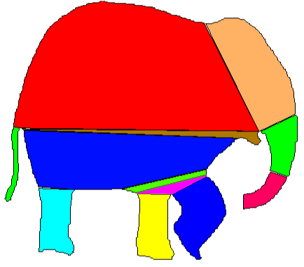
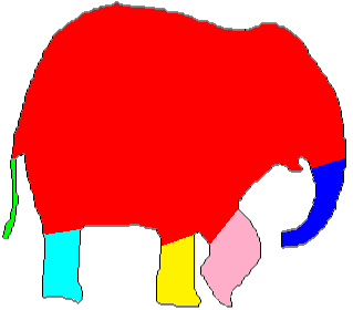
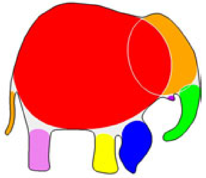
Figure 1: The decomposition process of an elephant shape (best viewed on screen). (a) The silhouette and skeleton of an elephant. (b) The simplified shape polygon (in red solid line) after using DCE, where the 13 concave vertexes are served as $\boldsymbol{m}$$-$ points of the origin shape contour. This process also helps in pruning redundant skeleton branches [2]. (c)-(d) single-minimum and double-minima part-cut hypotheses, those discarded and remaining ones are shown as blue dashed and red solid lines, respectively. (e)-(f) Decomposition results of the proposed method, [17], [18] and [22], respectively.

I-A Related work

The majority of existing shape decomposition approaches can be classified into two categories. One category aims to decompose shapes into near-convex parts. The other category tries to decompose shapes into natural parts based on psychophysics studies.

The first category usually decomposes shapes based on the convexity constraint. This is mainly because that convexity plays an important role in human perception [3], and is also supported by the minima rule. Conventional strict convex decomposition is a well-studied problem, but is not suitable in the case of shape decomposition. Because human may “see” a shape in different scales to find the most perceivable meaning of it. When we decompose a shape at a particular scale, non-convexity below that scale should be neglected. Latecki and Lakamper [15] thus developed the DCE algorithm to control the tolerance level of non-convexity, and decompose shapes with concave vertexes of the DCE-simplified shape polygon. Lien et al. [17, 19, 8] proposed Approximate Convex Decomposition (ACD), which decomposes shapes into approximately convex parts. Liu et al. [18] proposed Convex Shape Decomposition (CSD) by formulating the shape decomposition problem as an integer linear programming problem, which is further extended in [23, 12, 20], by introducing visual naturalness regularization terms into the object function.

The other category aims to decompose shapes into natural parts. Skeletons or local symmetric axes of shapes are usually involved according to the psychological model in [14]. Singh and Hoffman [26] defined a part-cut, the border line of two parts, as a straight line inside the shape that crosses an axis of local symmetry. Macrini et al. [21, 1] recognized the ligature in Blum’s skeleton [4] as the glue between parts and represented the part structure of a shape by a bone graph. Probabilistic approaches such as [29, 7] were proposed to provide a more robust estimation of the skeletal structure, which more faithfully represent the part structure. Other types of skeletons, such as shocks [13] and smoothed local symmetries (SLS) [5], have also been used. The limb and neck based method of [25] used shocks to extract necks and boundary curvature to find limbs. Mi and DeCarlo [22] argued that shapes should be decomposed by part transitions instead of part-cuts. They traced along the axes of SLS to find regions with strong transitional strength and decomposed shapes into overlapped parts. We have borrowed the idea of part transitions to define the neighborhood histogram, which is essential to our decomposition approach.

II Our Approach

The psychological study in [6] suggests that most subjects segment an object shape into parts on the basis of straight lines that start and end on the boundary, which are called the “part-cuts” of the shape. According to the conditions laid out in [26], a part-cut is “a straight line segment” that joins two points on the outline of a silhouette such that the following conditions are satisfied:

• at least one of the two points has negative curvature;

• the entire segment locates in the interior of the shape; and

• the segment crosses an axis of local symmetry.

Given a shape $X\subset\mathbb{R}^{2}$, together with a set of part-cuts $C=\{c_{1},c_{2},...,c_{N}\}$. The shape can be written as $X=\{P_{1},P_{2},...,P_{N+1}\}$, where $\forall i,1\leqslant i\leqslant N+1,P_{i}\subset\mathbb{R}^{2}$ is a visual part of $X$, and $P_{i}\cap P_{j}=c_{ij}\in C{\text{ or }}P_{i}\cap P_{j}=\emptyset,\forall i\neq j,1\leqslant i,j\leqslant N+1$. The problem that we are interested is how to obtain part-cuts $C$. The definition of “part-cuts” in [26] thus guides our work. We firstly find segmentation points on the basis of Condition ($a$), and then extract a set of part-cut hypotheses $H=\{h_{1},h_{2},...,h_{|H|}\}$ that are consistent with Condition ($b$). Here $|H|$ is the size of the set $H$. The set of part-cuts $C$ is chosen from $H$ with minimal total cost based on Condition ($c$) and the short-cut rule:

$$\mathop{\min}\limits_{C}\sum\limits_{i=1}^{N}{{\text{Cost}}(c_{i})},$$ (1)

where $c_{i}\in C$, and Cost($c_{i}$) is a positive quantity that represents the cost associated with the part-cut $c_{i}$.

Algorithm 1 Shape decomposition.

1

The overall framework of our algorithm is shown in Algorithm 1. Finally, the shape $X$ is decomposed into visual parts by part-cuts in $C$.

II-A Finding part-cut hypotheses

In this section, we present our approach for finding the part-cut hypotheses.

II-A1 Segmentation points

The minima rule suggests that human vision separates shape contours at $\boldsymbol{m}$$-$ points. Condition ($a$) above relaxes this constraint by allowing other geometric factors to play a role in parsing. Winter and Wagemans’ large-scale experiments [6] revealed that nearly $70\%$ of segmentation points are $\boldsymbol{m}$$-$ points. Based on this fact, we use $\boldsymbol{m}$$-$ as segmentation points. Since the contours of shapes are usually distorted by noise, we simplify the contour with a closed polygon in order to find $\boldsymbol{m}$$-$ points. This process does not significantly affect the final decomposition result as visual perception inherently allows some degree of deviation. DCE of [15] is one of the contour simplification methods that preserves perceptual appearance while eliminating distortions. As shown in Fig. 1, the noise in the outline of the top left silhouette generates a lot of redundant skeleton branches. After applying DCE, the contour of the elephant is represented as a polygon, in which the redundant skeleton branches are removed. As we will discuss later, the proposed algorithm is closely related to the skeleton (local symmetric axis) although the skeleton itself is never explicitly calculated. Within the polygonal silhouette generated by DCE, every concave vertex corresponds to a curvature minimum of the original shape. Rather than consider every such vertex, however, we introduce a threshold $\delta$, which is the minimal degree of concavity such that a vertex $p$ is considered to be an $\boldsymbol{m}$$-$ point only if its interior angle $\angle p>\pi+\delta$. This strategy simplifies computation and more importantly, tolerates the approximation error introduced by DCE. Taking perceptual salience and approximation error into account, we set $\delta=\frac{\pi}{9}$ in all of our experiments.

II-A2 Two types of cuts

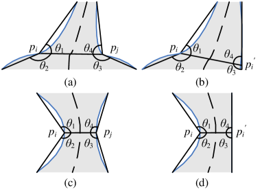
Figure 2: Angles formed by (a) limb, (b) neck, (c) limb-like single-minimum cuts, (d) neck-like single-minimum cuts and the simplified shape polygons. Limb and neck are both double-minima cuts. The left parts of the two shapes in (a), (b) and (c), (d) share the same geometry. $p_{i}p_{j}$ and $p_{i}p_{i}^{\prime}$ are of the same length.

August and Siddiqi in [1] suggested that the ligature and semi-ligature of [4] serve as the “glue” between parts, where a ligature related to two $\boldsymbol{m}$$-$ points defines a limb or a neck and a semi-ligature related to a single $\boldsymbol{m}$$-$ point divides a tail from the main body of the shape (see the elephant’s tail in Fig. 1 as an example). On this basis we partition the set of cuts into two classes based on the number of $\boldsymbol{m}$$-$ endpoints that they have. As shown in Fig. 2, limbs and necks, which have two $\boldsymbol{m}$$-$ endpoints, are called double-minima cuts. In contrast a single-minimum cut has only one $\boldsymbol{m}$$-$ endpoint. Following the idea of limb and neck, we further divide single-minimum cuts into neck-like single-minimum cuts and limb-like single-minimum cuts.

The two endpoints of a double-minima cut are both $\boldsymbol{m}$$-$ points. Therefore, each pair of $\boldsymbol{m}$$-$ points $p_{1}$ and $p_{2}$ represents a potential double-minima cut if the line segment connecting them meets Condition ($b$). This can be judged by checking if all pixels along $p_{1}p_{2}$ are inside the shape. The number of double-minima cuts must thus be less than $\binom{n}{2}$, with $n$ being the number of $\boldsymbol{m}$$-$ points.

The single-minimum cut has only one $\boldsymbol{m}$$-$ endpoint. Thus, if we draw a line from an $\boldsymbol{m}$$-$ to any arbitrary point on the shape contour, it can be considered as a potential single-minimum cut when meets Condition ($b$). The large number of possible cuts of this type makes the decomposition problem computationlly intractable. Next, we propose an approximate method.

For an $\boldsymbol{m}$$-$ point $p_{i}$ and a set of $n_{d}$ directions, we construct a set of $n_{d}$ potential part-cut hypotheses, each of which starts at $p_{i}$ and extends until it exits the shape. Let us suppose that a line intersects the contour at $p_{i}^{\prime}$. Then $p_{i}p_{i}^{\prime}$ is a single-minimum part-cut hypothesis. This approach is based on the observation that the human visual system does not work so accurately to differentiate part-cuts in very close directions. Therefore, as long as $n_{d}$ is sufficiently large (we find that $n_{d}=16$ suffices as shown in our experiments) and the directions are sampled evenly, the sampled $n_{d}$ potential part-cut hypotheses can serve as a good approximation of the entire single-minimum part-cut set. The number of extracted single-minimum cuts should be less than $n_{d}\cdot n$ because there may not exist any line segment lying inside the shape in some directions. Recall that $n$ is the number of $\boldsymbol{m}$$-$ points on the contour of a shape.

Moreover, if $p_{i}^{\prime}$ is sufficiently close to another $\boldsymbol{m}$$-$ point (w.l.o.g., labelled as $p_{j}$) along the contour, $p_{i}p_{i}^{\prime}$ is then merged with $p_{i}p_{j}$ and regarded as a double-minima cut. Here the “sufficiently-close” distance is set to be less than a threshold equalling to $\min\{1\%\cdot m,d_{\rm min}\}$. Here $m$ is the length of the contour in pixels, and $d_{\rm min}$ is the length of the shortest edge in the polygon. In [6] the authors have defined a similar threshold. This threshold allows for some noise in the segmentation data and at the same time rejects unlikely singularity points.

We present the process of finding part-cut hypotheses in Algorithm 2. The output of this algorithm are two sets: $V$ and $H$, which contain the segmentation points and the part-cut hypotheses, respectively.

Algorithm 2 Part-cut hypotheses extraction.

3

3

3

II-B Decomposing a shape into parts

After applying the two steps as described above, there are at most $\binom{n}{2}+n_{d}\cdot n$ part-cut hypotheses stored in $H$. The next step is to determine the “true” part-cuts from the hypotheses in $H$.

Let us assign a boolean variable $y_{j}\in\{0,1\}$, ($j=1,\cdots,|H|$), to each part-cut hypothesis in the set $H$, where $|H|$ is the size of the set $H$. $y_{j}=1$ means that the part-cut hypotheses with index $j$ is identified as a final cut; and $y_{j}=0$ indicates that the part-cut hypothesis $j$ is discarded. In general, we can formulate an optimization problem as follows:

$$\min_{y_{1},\cdots,y_{|H|}}\sum_{j}\psi_{u}(y_{j})+\sum_{jk}\psi_{v}(y_{j},y_{k}).$$ (2)

The first unary term is the energy modelling the compatibility of data with label $y_{j}$. The second term is the energy modelling the pairwise relationships. Since we do not have prior knowledge about the number of cuts for a particular shape, model selection criteria such as the Akaike information criterion may be used. Although it is possible to employ sophisticated optimization techniques such as integer programming to solve (2), which is generally a NP-hard problem, we seek a sub-optimal solution using a greedy pruning method.

Next we show how to properly define the two energy terms in (2) according to the short-cut rule and other psychophysics results, which is the core of our approach.

II-B1 Constraints from observations

Let us consider the unary energy term at first. The important fact is that a part-cut must satisfy some constraints that comply with visual perception. Here we formulate a few such fundamental constraints from observations which can be used to distinguish a part-cut from other candidates, mainly based on its local properties. It is to be highlighted that, due to the flexibility of our framework, it is easy to accommodate more constraints with minimal modification to the overall framework.

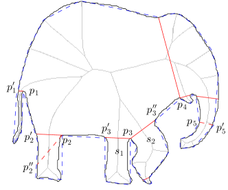
Figure 3: Illustration of observations on the elephant shape. The part-cuts shown in red solid lines all cross a skeleton (axis of local symmetry) almost orthogonally (Observation 1), and have at least one “expanding” sides (Observation 3). Each $\boldsymbol{m}$$-$ point can have two part-cuts at most, e.g., $p_{3}$ and $p_{4}$ both have two part-cuts (Observation 2). The single-minimum part-cut hypothesis $p_{5}p_{5}^{\prime}$ is discard due to Observation 4. Skeletons of the shape are shown for interpretation, but they are never computed.

Observation 1: A part-cut must cross an axis of local symmetry ‘almost orthogonally’.

This observation is a strict version of Condition ($c$) of part-cuts as introduced in [26]. The requirement of ‘crossing almost orthogonally’ is a result of the short-cut rule. Because the orthogonal ribs are usually the shortest cuts along the axis of local symmetry. See the toy example of $p_{2}p_{2}^{\prime}$ and $p_{2}p_{2}^{\prime\prime}$ in Fig. 3.

Observation 2: For every $\boldsymbol{m}$$-$ point, there are at most two part-cuts going through it.

As illustrated in Fig. 3, $p_{3}$ may relate to at most two axes of local symmetry—$s_{1}$ corresponded to the left side of $p_{3}$ and $s_{2}$ corresponded to the right side. For each axis, only the shortest cut, which orthogonally crosses the axis, is kept according to Observation 1.

Observation 3: At least one side of a part-cut should be expanding.

The term “expanding”, whose counterpart is “shrinking”, means that departing from the part-cut in one side, local widths (the lengths of ribs along the axis of local symmetry) of the shape getting larger. Observation 3 is a complement of Observation 1. It is based on the fact that, if both sides are shrinking, the cut must be a local maximum of local width, which contradicts the short-cut rule. Clearly, if both sides of a part-cut are expanding, it is a neck or a neck-like single-minimum part-cut (Fig. 2(b) and (d)). Otherwise, it is a limb or a limb-like single-minimum part-cut (Fig. 2(a) and (c)).

Observation 4: A single-minimum part-cut should be salient.

This observation, which has its origin in [22], is used to prevent noise on the outline of a shape. Unlike the double-minima part-cut hypothesis, a single-minimum hypothesis has only one $\boldsymbol{m}$$-$ end. If this end is caused by noise, it is less likely to be a conspicuous boundary of two parts. Therefore, we need to conduct further investigation to check the salience of a single-minimum hypothesis to be a part-cut. It can also distinguish bending from joint of two parts. See Fig. 3 for example, $p_{5}p_{5}^{\prime}$ is rejected since it is insufficient salient to decompose the trunk, while $p_{1}p_{1}^{\prime}$ is accepted due to its strong segmentation effect in cutting the tail off from the body.

II-B2 Implementation of constraints

Now with these observations, we can define the unary energy term in problem (2). Given a particular part-cut hypothesis $y_{j}$, if it violates any of the observations, its energy cost $\psi_{u}(y_{j})$ is set to be very large. In other words, we set $y_{j}=0$ and this part-cut hypothesis must be excluded.

Here a problem is that all the observations except Observation 2 are qualitative descriptions instead of computable constraints. Here we propose to use the simplified shape polygon and the local information of the part-cut hypotheses to implement Observations 1, 3 and 4.

For Observations 1 and 3, local symmetric axes are involved. Since the cost to compute the local symmetric axis is expensive, we use the simplified shape polygon to implement these two observations. In Fig. 2, each part-cut hypothesis forms four angles with the polygon. For any hypothesis, the upside (downside) of which is expanding if and only if $\theta_{1}+\theta_{4}>\pi$ (or, $\theta_{2}+\theta_{3}>\pi$). Meanwhile, $\theta_{1}$ and $\theta_{4}$ (or, $\theta_{2}$ and $\theta_{3}$) are approximately equal per the requirment of Observation 1. Therefore, in practice, we state that a part-cut hypothesis satisfies Observations 1 and 3 if either $\theta_{1},\theta_{4}>\frac{\pi}{2}-\delta$ or $\theta_{2},\theta_{3}>\frac{\pi}{2}-\delta$ holds. Here $\delta$ is a constant as defined in Section II-A1.

For Observation 4, the quantitative definition of “salience” is required. Mi and DeCarlo [22] discussed the salience of a part-cut hypothesis in detail. By borrowing their idea of transition strength, here we construct the neighborhood histogram for each single-minimum hypothesis in order to properly measure the salience of a single-minimum hypothesis.

As shown in Fig. 4, the $y$-axis in each plot is a single-minimum part-cut hypothesis. We draw a straight line in parallel to the $y$-axis for every $\hat{\sigma}$ pixels along the $x$-axis within a distance of $\pm{\sigma}$ pixels. Here $\sigma$ is the radius of neighborhood. Lengths of line segments inside the shape then construct the neighborhood histogram of the part-cut hypothesis, as shown at the bottom row of Fig. 4. Since a cut is orthogonal to the axis of local symmetry, these parallel line segments are also approximately orthogonal to the axis of local symmetry, based on the following two facts—the size of neighborhood $\sigma$ is small, and the axis of local symmetry is generally locally smooth [9]. In other words, they can approximately be seen as ribs of the axis. Thus the neighborhood histogram reveals the variation of the local width near the part-cut hypothesis. It is clear that the more significant the local width near a single-minimum part-cut hypothesis varies, the more salient it is.

On the other hand, to fulfill the requirement of Observation 3, at least one side of its neighborhood histogram should monotonically increase from the origin. In particular, if both sides increase as in Fig. 4(a), it is neck-like, and the more rapid they increase, the more salient it is. If only one side increases as in Fig. 4(b), it is limb-like, and the higher the two sides contrast, the more salient it is. We hereby use the statistics of the neighborhood histogram to measure the salience of a single-minimum hypothesis $h_{j}$. It is said to be salient if 1) $\frac{\sigma_{j}}{\mu_{j}}>t_{h1},l_{j}<\mu_{j}$ or 2) $\max\left\{\frac{\mu_{j}^{-}}{\mu_{j}^{+}},\frac{\mu_{j}^{+}}{\mu_{j}^{-}}\right\}>t_{h2},l_{j}<\mu_{j}$, where $\mu_{j}$ and $\sigma_{j}$ are the mean and standard deviation of the entire histogram. $\mu_{j}^{-}$ and $\mu_{j}^{+}$ are means of the histogram’s two halves. $t_{h1}$ and $t_{h2}$ are thresholds for salience. $l_{j}$ is the length of $h_{j}$ and $l_{j}<\mu_{j}$ is due to the requirement of the short-cut rule. The term $\max\left\{\frac{\mu_{j}^{-}}{\mu_{j}^{+}},\frac{\mu_{j}^{+}}{\mu_{j}^{-}}\right\}$, which measures the “expansion” from one side of $h_{j}$ to the other side, is specially introduced for limb-like hypotheses. We regard that if the size expands two times from one side to the other, it could be consider as salient part-cut hypothesis, and thus set $t_{h2}=2$. The setting of $t_{h1}$ is discussed in the experiments (Section III). To support these statistic criteria, the radius of neighborhood $\sigma$ must be large enough. We find $\sigma=5\hat{\sigma}$ is fine in experiments.

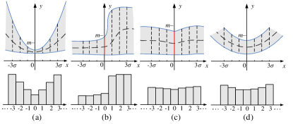
Figure 4: Neighborhood histograms (bottom row) of single-minimum part-cut hypotheses (top row), where (a) and (b) change significantly while (c) and (d) are stable.

Furthermore, we know that there are at most two part-cuts for every $\boldsymbol{m}$$-$ point according to Observation 2, and shorter candidates are more likely to be selected as part-cuts according to the short-cut rule. To further reduce the number of part-cut hypothesis, we keep, at most, the shortest two double-minima part-cut hypotheses as well as the shortest two single-minimum part-cut hypotheses for each $\boldsymbol{m}$$-$ points. This approximation seems not to compromise the accuracy, but reduces the number of part-cut hypotheses to examine in the next stage. Therefore, for each $\boldsymbol{m}$$-$ points, we keep at most four part-cut hypotheses as the candidates, from which at most two can be selected as true part-cuts due to Observation 2. Now, the number of part-cut hypotheses is no more than $4n$.

II-B3 Determination of part-cuts

The short-cut rule states that the cut length is a critical measure in deciding part-cuts. However, as shown in Fig. 2, although shapes in each row share the same length of cuts and the same geometry on the left side, it appears that the strength of $p_{i}p_{j}$ partitioning the shape is stronger than that of $p_{i}p_{i}^{\prime}$ partitioning the shape. Mi and DeCarlo introduced the notion of transition strength to describe this effect in [22]. Their results suggest that the segmentation strength of a single-minimum cut is about half of a double-minima cut. Therefore, we introduce the relative length to encode this difference. For a part-cut hypothesis $h_{j}$ with length $l_{j}$, its relative length ${{\widetilde{l}}}_{j}$ is defined as:

$${{\widetilde{l}}}_{j}=\left\{{\begin{array}[]{*{20}l}{\frac{{l_{j}}}{R}},&{{h_{j}\text{ is a {double-minima} cut,}}}\\ {2\frac{{l_{j}}}{R}},&{h_{j}{\text{ is a {single-minimum} cut,}}}\\ \end{array}}\right.$$ (3)

where $R$ is the radius of the shape’s minimum enclosing disk for normalization.

The energy of a part-cut hypothesis $h_{j}$ is a function of this relative length; i.e.,

$$\psi_{u}(y_{j})\equiv f({{\widetilde{l}}}_{j}).$$

Here $y_{j}$ is the label of $h_{j}$, and $f(\cdot)$ is a monotonically increasing function since a shorter cut should carry lower energy and is always preferred. Since we use a greedy method that approximately solve the original NP-hard problem (2), we do not need to know the explicit form of $f(\cdot)$. Instead we sort $h_{j}$ by values of $f({{\widetilde{l}}}_{j})$, which can be simply achieved by sorting ${{\widetilde{l}}}_{j}$, $\forall j$.

The term $\psi_{v}(y_{j},y_{k})$ in (2) models the pairwise relationship between $h_{j}$ and $h_{k}$. To ensure the visual parts are non-overlapped, the selected part-cuts should not intersect with each other. If two part-cut hypotheses intersect with each other, they are “in conflict”. There are some other specific cases of conflict between two part-cut hypothese.

If two hypotheses $h_{j},h_{k}$ are in conflict, they cannot be selected simultaneously. Mathematically it means $y_{j}\cdot y_{k}=0$. We can set the pairwise energy term $\psi_{v}(y_{j}=1,y_{k}=1)$ to be extremely large. If two hypotheses are compatible, the pairwise energy is set to zero.

Algorithm 3 Part-cut determination.

2

2

The part-cut determination process is illustrated in Algorithm 3. Part-cut hypotheses are sorted by their relative lengths in ascending order. Those single-minimum ones are usually put in the rear of the examining queue due to their larger relative lengths. If the current part-cut hypothesis does not violate Observation 2 and is not in conflict with any determined part-cuts, it is accepted. Part-cut hypotheses with shorter relative lengths are at the front of the queue, therefore are preferred by the selection procedure. This can be viewed as the simplified implementation of the short-cut rule.

II-C Time complexity analysis

To analyze the time complexity of the proposed approach, our method must be divided into two stages—the simplification of the contour, and the determination of the part-cuts.

The first stage is done using DCE [15], which has been shown to be $O(m\log m)$ in time complexity [16].

The most expensive computation in stage two is to judge whether a cut is inside the shape (the neighborhood histogram can be constructed at the same time) and to resolve conflicts between part-cut hypotheses. The former process consumes at most $O((\binom{n}{2}+n_{d}n)R)$ time when the number of cuts is less than $\binom{n}{2}+n_{d}n$ and the lengths of them are shorter than the radius of the shape’s minimum enclosing disk $R$. The latter process needs $O((4n)(2n))$ time since the number of elements in $H^{\prime}$ and $C$ is less than $4n$ and $2n$, respectively. So the total time complexity of this stage is $O(n^{2}R)$.

Since $R$ is smaller than $m$, the total time complexity is $O(m\log m+n^{2}R+m)=O(m(n^{2}+\log m))$.

The work of [17], [18], [22], and [23] represents the most recent development for shape decomposition. The work of [22] needs to identify SLS of the shape, which is $O(m^{2})$. The most time-consuming part of [18] and [23] is $O(t\log t)$, where $t$ is the number of pixels of the silhouette which is much larger than $m$ (in quadratic). As demonstrated in the next section, $n$ is always small (in dozens) in our experiments. Therefore the time complexity of our proposed method is lower than [18, 23, 22] in general. The work of [17] is designed for approximate convex decomposition of polygons and is very fast ($O(mr)$, where $r$ is the number of notches of the polygon). However, our method obtains more intuitive decomposition results than [17] as shown in the experiments.

The average computational costs, on a standard dual-core desktop computer, of [22], [18] and the proposed method in the experiments of Sec. III-A are 0.0048s, 10.89s and 0.1566s, respectively. Note that the experiments of [22] used the well optimized C++ code provided by the author, while the other two are both implemented in Matlab. The average decomposition time of [23] is 45.6s according to the authors. Those empirical computational results are consistent with the theoretical complexity analysis.

III Experimental Results

III-A Quantitative evaluation

Same as in image segmentation, evaluation of shape decomposition algorithms has been subjective, to an large extent. One usually has to judge the efficacy of a method by inspection of a small number of examples. Largely this is because shape decomposition itself is not a well-defined problem—one is not able to find a unique ground-truth decomposition of a shape, against which the output of an algorithm can possibly be compared. That may be the main reason why no quantitative evaluation was provided in shape decomposition work such as [18, 22, 23].

De Winter and Wagemans [6] have conducted a large-scale psychological study on how humans segment object shapes into parts based on a subset of Snodgrass and Vanderwart’s everyday object data set (S & V data set) [28], which could help us to evaluate the decomposition results with human behavior.

S & V data set consists of 260 line drawing of everyday objects, 88 of which were selected and converted into outline shapes as the stimulus materials to be decomposed by 201 subjects (first-year university students). Each subject is asked to segment a set of figures into parts by drawing lines (either straight or curved but straight lines were reported in [6] when most of the drawn lines were straight). One example of drawn lines from all subjects on a “glass” is shown in Fig. 5(a). We see that most subjects share the same opinion to separate the glass around the two joints of the stem, while a few others hold different views. To integrate opinions from all subjects, we propose to construct the segmentation density map for every shape with a Gaussian mixture like model. The segmentation density in any pixel $x_{i}$ of a shape is the accumulation of all drawn lines:

$$q(x_{i})=\sum\limits_{j}{q_{j}(x_{i})=\sum\limits_{j}{\exp(\frac{{-d_{j}^{2}(x_{i})}}{{\sigma^{2}}})}},$$ (4)

where $d_{j}(x_{i})$ is the distance from $x_{i}$ to the $j$th drawn line, $\sigma$ is the radius to construct neighborhood histogram in Sec. II-B2.

Fig. 6 presents some shapes decomposed by the proposed method and their segmentation density maps from S & V dataset. It is shown that most part-cuts lie on high density areas. Next we propose a criterion to evaluate the quantitative performance of a decomposition algorithm.

Given a set of part-cuts $C$ on the shape, we say a pixel is masked if it is within the distance of $3\sigma$ (due to the well-kown “Three-sigma rule”) to any part-cut. Let

$$\begin{array}[]{l}\mu_{{\rm{masked}}}=\mathop{{\rm{mean}}}\limits_{\exists j,D_{j}(x_{i})\leq 3\sigma}q(x_{i}):\mathop{\text{mean}}\limits_{x_{i}}q(x_{i}),\\ \mu_{{\rm{unmasked}}}=\mathop{{\rm{mean}}}\limits_{\forall j,D_{j}(x_{i})>3\sigma}q(x_{i}):\mathop{\text{mean}}\limits_{x_{i}}q(x_{i}),\\ \end{array}$$ (5)

where $D_{j}(x_{i})$ is the distance from $x_{i}$ to the $j$th part-cut. The larger $\mu_{\text{masked}}$ is, the better $C$ is compatible with the drawn lines; and the smaller $\mu_{\text{unmasked}}$ is, the more drawn lines $C$ covers. That is, $\mathcal{H}=\mu_{\text{masked}}:\mu_{\text{unmasked}}$ represents the overall similarity between $C$ and the experimental results of [6] (higher is better). However, a large number of part-cuts, covering a major proportion of the shape, may lead to a very small $\mu_{\text{unmasked}}$. Then $\mathcal{H}$ is significantly high even when $C$ is not quite compatible with the drawn lines. So, as a precondition, the number of part-cuts $|C|$ should be roughly consistent with the psychophysical results, which is $3.97$ per shape (22 shapes and $68.6$ drawn lines per subject with 21.4% “error” lines uncounted).

Figure 5: (a) Segmentation lines drawn by subjects in De Winter and Wagemans’ experiments. (b) Segmentation density map. (c) Part-cuts and their masking area. (d) Masked segmentation density map.

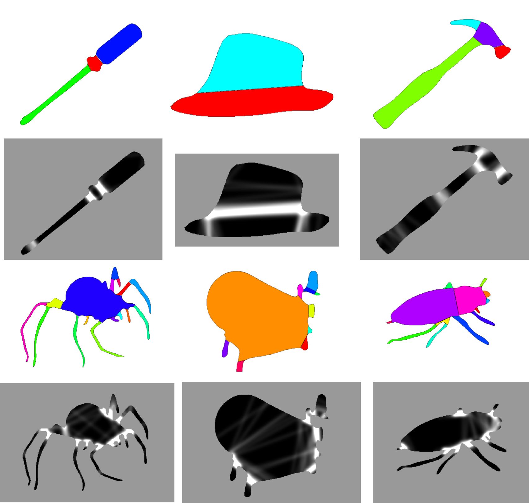
Figure 6: Decomposition of some shapes from S & V dataset (pseudocolor image), and their segmentation density maps (grey-scale image).

We compare the performance of three methods by average values on S & V data set in Table I. It is clear that the proposed method is more accordant with the experimental results of [6]. Surprisingly, the method in [18] performs much worse than the others. One possible reason may be the absence of visual naturalness in its definition of concavity.

TABLE I: Comparison of decomposition results on S & V data set. $\overline{\mathcal{H}}$ represents the overall similarity between $C$ and human decomposition. Higher is better.

Method	$\overline{|C|}$	$\overline{\mu_{\text{masked}}}$	$\overline{\mu_{\text{unmasked}}}$	$\overline{\mathcal{H}}$
ACD [17]	4.18	3.49	0.69	6.85
CSD [18]	3.80	3.09	0.78	4.72
Ours	4.07	3.77	0.66	8.54

III-B Evaluation of parameters

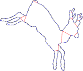
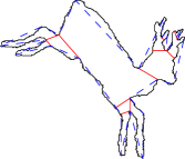
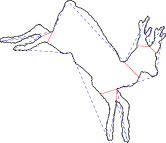
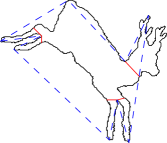
Figure 7: The decomposition results by the proposed method, with (a) $t_{\text{DCE}}=0.1$, (b) $t_{\text{DCE}}=0.5$, (c) $t_{\text{DCE}}=1$ and (d) $t_{\text{DCE}}=3$, respectively. The simplified polygons are in blue dashed lines while the determined part-cuts are in red solid lines.

A number of parameters have been introduced in our algorithm, which is a caveat of the proposed method. This is mainly because that human visual perception is a complicated process involving a lot of different (even conflicting, sometimes) principles [26], which can hardly be explained by several simple formulas. Nevertheless, most parameters possess clearly defined perceptual meanings and have been discussed accordingly when they are introduced. Other parameters include the stopping parameter $t_{\text{DCE}}$ of DCE, the number of directions $n_{d}$ for generating single-minimum part-cut hypotheses, and the threshold $t_{h1}$ associated with the neighborhood histogram.

The parameter $t_{\text{DCE}}$ tells how similar the simplified polygon with the origin shape boundary. Most discussions in Section II are based on the assumption that the polygon obtained by DCE is an approximate version of the shape’s boundary. Thus, $t_{\text{DCE}}$ should be small to maintain a high degree of similarity. We examine the impact of this parameter on the final performance of our method. As shown in Fig. 7, the proposed method works well for different values of $t_{\text{DCE}}$. With a small $t_{\text{DCE}}$, the detail of the shape boundary is kept, which in general introduces a large number of small parts. When the value of $t_{\text{DCE}}$ increases, the decomposition tends to miss more detail parts and tolerate more distortions at the same time.

Fig. 8(c) summaries the impact of $t_{\text{DCE}}$ on the performance on the S & V data set. The average number of part-cuts $\overline{|C|}$ is always not far from the psychophysical result of 3.97. The highest $\overline{\mathcal{H}}$ is obtained (with $t_{\text{DCE}}$ around 0.1) when $\overline{|C|}$ approximately fits it. It also shows that the average number of $\boldsymbol{m}$$-$ points $\overline{n}$ is always small (less than 20), which guarantees the low complexity of the proposed algorithm.

For comparison, we also plot the influence of $\tau$ to ACD and $\epsilon$ to CSD ($\tau$ and $\epsilon$ are both thresholds for concavity similar to $t_{\text{DCE}}$) in Fig. 8 (a) and (b), respectively. In (a), $\overline{|C|}$ is very large at a small $\tau$ and decreases almost exponentially when $\tau$ increases. The highest $\overline{\mathcal{H}}$ is obtained when $\overline{|C|}$ is three times larger than the psychophysical results. It is lower when $\overline{|C|}$ reaches 3.97 with $\tau$ being around 10. In (b), $\overline{\mathcal{H}}$ keeps lower than 5, and $\overline{|C|}$ reaches 3.97 with $\epsilon$ being around 0.03.

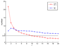
(a) ACD [17]

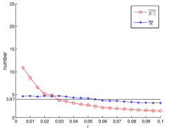
(b) CSD [18]

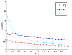
(c) Ours

Figure 8: Impact of the convex parameters for the three algorithms on the S & V data set.

We also evaluate the influence of the other two parameters $n_{d}$ and $t_{h1}$ on the S & V data set. In the experiments, $n_{d}$ varies from 8 to 32 with an increase of 8 at each step and $t_{h1}$ ranges from 0.2 to 0.8 with an increase of 0.2 at each step.

The results are reported in Table II. For $\overline{\mathcal{H}}$, the higher is better, and for $\overline{|C|}$, the closer to 3.97 is better. The best parameter settings are $n_{d}=8$ and $t_{h1}=0.4$. We can see that $n_{d}=16$ is usually sufficient for generating single-minimum part-cut hypotheses. When $n_{d}>16$, not only the complexity increases, but the decomposition results are also less consistent with the psychological results.

TABLE II: The score of $\overline{\mathcal{H}}$ (left) and $\overline{|C|}$ (right) for the S & V data set based on different pairs of parameters.

	$8$	$16$	$24$	$32$
$0.2$	8.48 / 4.23	8.44 / 4.51	8.40 / 4.61	8.51 / 4.82
$0.4$	8.59 / 3.93	8.54 / 4.07	8.59 / 4.23	8.35 / 4.32
$0.6$	8.33 / 3.86	8.35 / 3.95	8.34 / 4.08	8.10 / 4.18
$0.8$	8.33 / 3.78	8.28 / 3.91	8.24 / 3.98	8.01 / 4.10

III-C More results

To further evaluate the visual naturalness of the proposed algorithm, we compare the decomposition results of [22], [18], [17] and our method in Fig. 9. As we can see, the first and the fourth row produce similar and intuitive results, while the second and the third row may parse a long bend (e.g., the tail of the kangaroo) into parts.

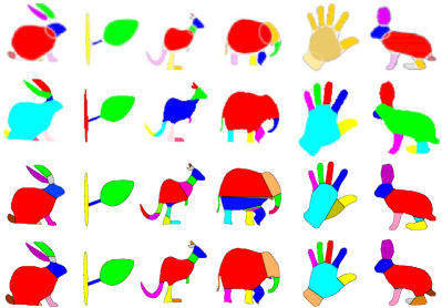
Figure 9: From top to bottom: decomposition results of [22], [18], [17] and our method.

Fig. 10 compares the decomposition results of some shapes from the MPEG-7 shape database produced by ACD [17], CSD [18] and our method. It can be seen that our method produces less part-cuts and the results are more natural.

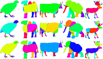
Figure 10: From top to bottom: decomposition results of some shapes from MPEG-7 shape database by [18], [17] and our method.

Fig. 11 demonstrates the robustness of our method in the presence of noise, occlusion, articulation and rotation. We deal with noise by increasing $t_{\text{DCE}}$. As in the first column, the noised “T” shape is firstly de-noised to a closed polygon (drawn in red lines) and then decomposed into two parts. We also see that occlusion in the second column does not affect the decomposition process in the un-occluded part of the shape. In the third column, the left hand of the man in the right column moves around his shoulder. Our method separates it from his body in both cases. In the last column, we can see that the angle of the single-minimum part-cut alters slightly. This is because we only generate single-minimum part-cut hypotheses in $n_{d}$ directions. However, this alteration does not have a significant impact on the performance when $n_{d}$ is set to a sufficiently large value.

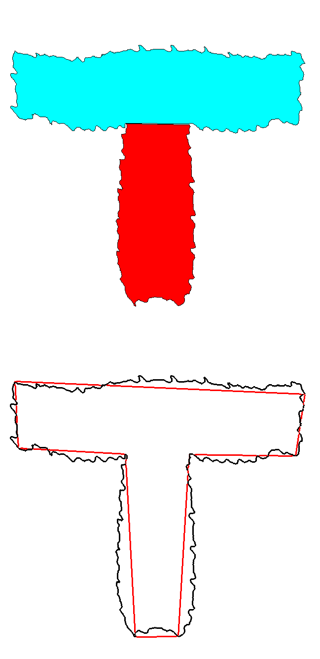
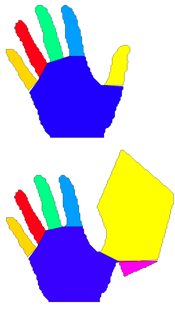
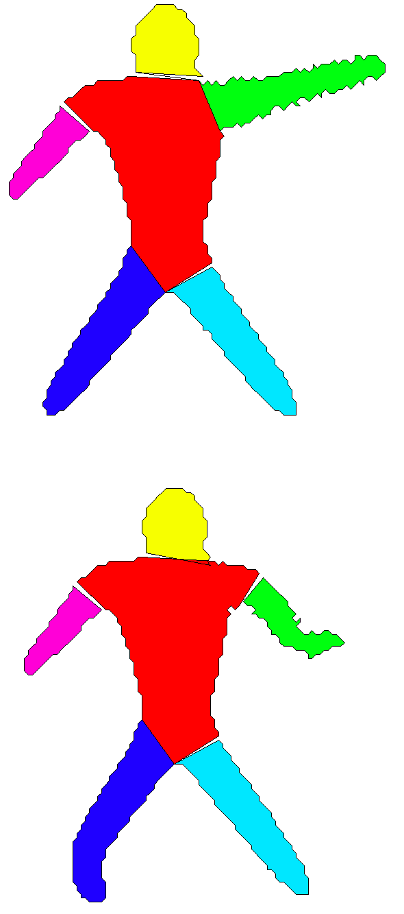
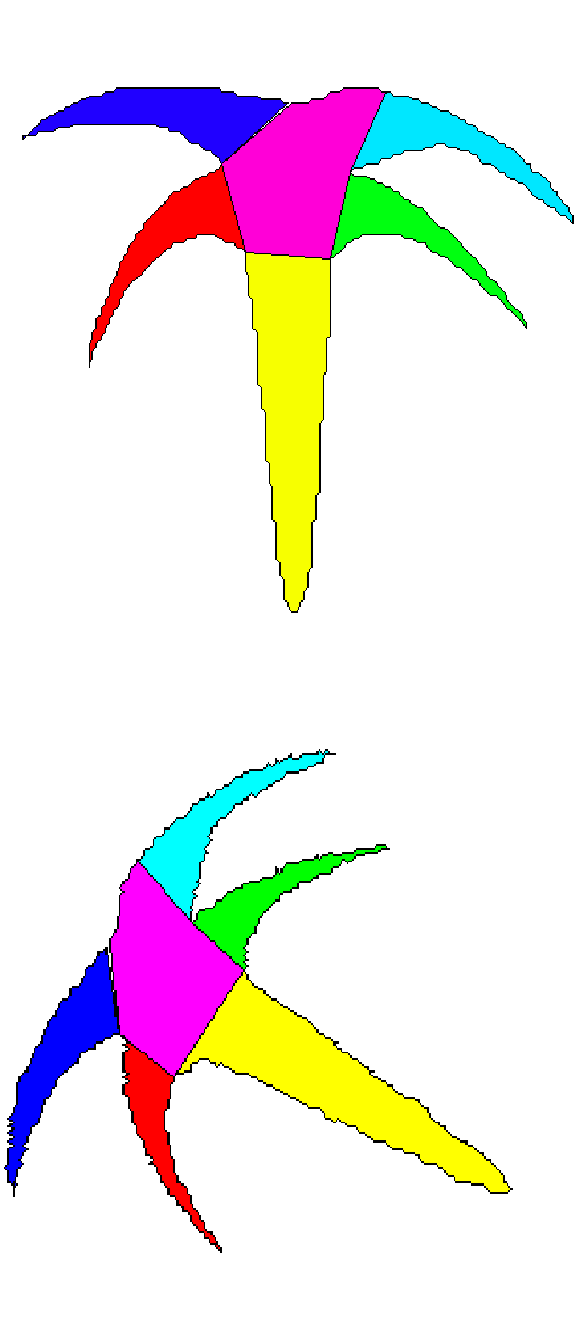
Figure 11: Decomposition examples in the presence of (a) noise, (b) occlusion, (c) articulation and (d) rotation.

III-D Hand gesture recognition

We now demonstrate the efficiency of the proposed algorithm by applying it to hand gesture recognition. Following the setting in [23], the task is to recognize hand gestures of three categories, namely Rock, Paper and Scissors. The data set, including both color images and depth maps, is collected by a Kinect depth camera. Each category has 100 samples collected from 10 subjects. As shown in Fig. 12, with the help of depth maps, hand shapes are easy to be segmented, although not perfectly, from the scenes. We then decompose them by the proposed algorithm. Fig. 13 shows some decomposition results of hand gestures from different subjects under various scale, orientation and illumination conditions. Similar to [23], we classify a gesture to Rock if $k\leq 2$, Paper if $k\geq 5$, and Scissors otherwise, where $k$ is the number of parts. With the setting of $t_{\text{DCE}}=1.2$, the proposed method perfectly distinguishes all of these 300 gestures into correct categories comparing with [23] whose mean recognition accuracy is 94.7% on a even smaller set.

Figure 12: Illustration of the hand gesture recognition experiment. From left to right: the color image, the depth image, the extracted hand shapes and the decomposition result.

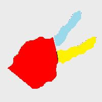
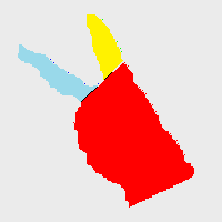
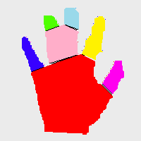
Figure 13: Hand gesture decomposition results. Although shapes in the last column are not decomposed perfectly, they can still be discriminated from other categories by counting the number of parts.

IV Conclusion

In this work, we have proposed a new flexible shape decomposition approach based on the short-cut rule, which roots in psychology. In other words, we have proffered a computational procedure of the short-cut rule, and applied it to 2D shape decomposition. An important component of the proposed approach is that we divide the potential cuts of a shape into two types according to the number of $\boldsymbol{m}$$-$ points that they have. We then examine them in order from shortest to longest to determine part-cuts, based on the short-cut rule.

Experiments show that our method can separate shapes into intuitive parts with low time complexity. Our approach can also be improved easily by introducing more constraints from visual observations. Although a few parameters are involved in our model, we empirically show that the final performance is not very sensitive to these parameters in a large range. We will explore the possibility of automatically tuning these parameters by computing a measure of salience for part-cut hypotheses with the definition proposed by [11].

Appendix A Discrete Curve Evolution

The Discrete Curve Evolution (DCE) algorithm was introduced in [15] to obtain shape hierarchy for multiscale shape analysis. Contours of shapes are usually distorted by digitization noise. DCE regards a shape contour as a polygon with a large number of vertices, and simplifies it with an evolution process to eliminate distortions. The evolution process is done according to a criterion $K(\cdot,\cdot)$ measuring the significance of two consecutive edges’ contribution to the shape:

$$K(s_{1},s_{2})=\frac{\beta(s_{1},s_{2})l(s_{1})l(s_{2})}{l(s_{1})+l(s_{2})},$$ (6)

where $\beta(s_{1},s_{2})$ is the turn angle at the common vertex of $s_{1},s_{2}$, $l(\cdot)$ is the normalized length of an edge. The higher value $K(s_{1},s_{2})$ is, the larger $s_{1},s_{2}$ contribute to the shape. In each evolutional step, the pair of consecutive edges with minimum $K$ value is selected to be replaces with a new line segment joining the endpoints of them. The evolution will converge to a convex polygon. If a termination threshold $t_{\text{DCE}}$ is given, it stops when no $K$ value is less than $t_{\text{DCE}}$. An illustration of the procedure is shown in Fig. 7, where the simplified polygon (in blue dashed lines) of the deer getting rougher as $t_{\text{DCE}}$ inceases. In general, DCE is a greedy approach to simplify the contour while keeping its geometric structure as much as possible. See [15, 16] for more details about the DCE algorithm.

Appendix B Illustration of Observations 3

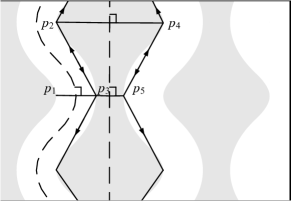
Figure 14: Parallelism (white) and co-circularity (grey). The grey “dumbbell” is simplified into a polygon by DCE. $p_{1}p_{3},p_{2}p_{4}$ and $p_{3}p_{5}$ both are orthogonal to the local symmetry axis (dashed line), while $p_{3}p_{5}$ is more likely to be a part-cut.

We here give a detailed explanation of the term of “expanding” in Observation 3. In an arbitrary shape, two types of local symmetry—parallelism and co-circularity—may appear. As illustrated in Fig. 14, the outline of the white “wiggle” is parallel, and the gray “dumbbell” is mirror symmetric, or co-circular. The length of the rib along the axis of local symmetry, or the local width, of the wiggle keeps unchanged, while it varies with the co-circular outline of the dumbbell. Previous research [13, 24] suggested that the human vision system does not tend to parse the wiggle into parts. Thus only the symmetry of co-circularity is considered here. Giblin and Brassett [9] proved that the axes of local symmetry generally are smooth curves. It means that the local width of the (co-circular) boundary, starting from a cut which is orthogonal to the axis of local symmetry, may vary continuously in two trends—expanding or shrinking. As shown in Fig. 14, departing from $p_{3}p_{5}$, either upwards or downwards, the trend is expanding, while it is shrinking from $p_{2}p_{4}$. In general, “expanding” and “shrinking” are the description of the varying trends of local width near the part-cut hypothesis.

References

- [1] J. August, K. Siddiqi, and S. W. Zucker. Ligature instabilities in the perceptual organization of shape. Comp. Vis. Image Understanding, 76(3):231–243, 1999.
- [2] X. Bai, L. J. Latecki, and W.-Y. Liu. Skeleton pruning by contour partitioning with discrete curve evolution. IEEE Trans. Patt. Anal. Mach. Intell., 29(3):449–462, 2007.
- [3] R. Basria, L. Costab, D. Geigerc, and D. Jacobsd. Determining the similarity of deformable shapes. Vision Research, 38:2365–2385, 1998.
- [4] H. Blum and R. N. Nagel. Shape description using weighted symmetric axis features. Pattern Recogn., 10(3):167–180, 1978.
- [5] M. Brady and H. Asada. Smoothed local symmetries and their implementation. Int. J. Robotics Research, 3:36–61, 1984.
- [6] J. De Winter and J. Wagemans. Segmentation of object outlines into parts: A large-scale integrative study. Cognition, 99(3):275–325, 2006.
- [7] J. Feldman and M. Singh. Bayesian estimation of the shape skeleton. Proceedings of the National Academy of Sciences, 103(47):18014–18019, 2006.
- [8] M. Ghosh, N. M. Amato, Y. Lu, and J.-M. Lien. Fast approximate convex decomposition using relative concavity. Computer-Aided Design, 45(2):494–504, 2013.
- [9] P. J. Giblin and S. Brassett. Local symmetry of plane curves. The American Mathematical Monthly, 92(10):689–707, 1985.
- [10] D. D. Hoffman and W. A. Richards. Parts of recognition. Cognition, 18:65–96, 1984.
- [11] D. D. Hoffman and M. Singh. Salience of visual parts. Cognition, 63(1):29–78, 1997.
- [12] T. Jiang, Z. Dong, C. Ma, and Y. Wang. Toward perception-based shape decomposition. In Proc. Asian Conf. Comp. Vis., pages 188–201, 2012.
- [13] B. B. Kimia, A. R. Tannenbaum, and S. W. Zucker. Shape, Shocks and Deformations I: The components of two-dimensional shape and the reaction-diffusion space. Int. J. Comp. Vis., 15(3):189–224, 1995.
- [14] I. Kovács and B. Julesz. Perceptual sensitivity maps within globally defined visual shapes. Nature, 370(6491):644–646, 1994.
- [15] L. J. Latecki and R. Lakamper. Convexity rule for shape decomposition based on discrete contour evolution. Comp. Vis. Image Understanding, 73(3):441–454, 1999.
- [16] L. J. Latecki and R. Lakamper. Application of planar shape comparison to object retrieval in image databases. Pattern Recogn., 35(1):15–29, 2002.
- [17] J.-M. Lien and N. M. Amato. Approximate convex decomposition of polygons. Computational Geometry, 35(1):100–123, 2006.
- [18] H. Liu, W. Liu, and L. J. Latecki. Convex shape decomposition. In Proc. IEEE Conf. Comp. Vis. Patt. Recogn., 2010.
- [19] Y. Lu, J.-M. Lien, M. Ghosh, and N. M. Amato. -decomposition of polygons. Computers & Graphics, 36(5):466–476, 2012.
- [20] C. Ma, Z. Dong, T. Jiang, Y. Wang, and W. Gao. A method of perceptual-based shape decomposition. In Proc. IEEE Int. Conf. Comp. Vis., 2013.
- [21] D. Macrini, K. Siddiqi, and S. Dickinson. From skeletons to bone graphs: Medial abstraction for object recognition. In Proc. IEEE Conf. Comp. Vis. Patt. Recogn., 2008.
- [22] X. Mi and D. DeCarlo. Separating parts from 2D shapes using relatability. In Proc. IEEE Int. Conf. Comp. Vis., 2007.
- [23] Z. Ren, J. Yuan, C. Li, and W. Liu. Minimum near-convex decomposition for robust shape representation. In Proc. IEEE Int. Conf. Comp. Vis., 2011.
- [24] H. Rom and G. Medioni. Hierarchical decomposition and axial shape description. IEEE Trans. Patt. Anal. Mach. Intell., 15(10):973–981, 1993.
- [25] K. Siddiqi and B. B. Kimia. Parts of visual form: Computational aspects. IEEE Trans. Patt. Anal. Mach. Intell., 17(3):239–251, 1995.
- [26] M. Singh and D. D. Hoffman. Part-based representations of visual shape and implications for visual cognition. Advances in Psychology, 130:401–459, 2001.
- [27] M. Singh, G. D. Seyranian, and D. D. Hoffman. Parsing silhouettes: The short-cut rule. Perception & Psychophysics, 61:636–660, 1999.
- [28] J. G. Snodgrass and M. Vanderwart. A standardized set of 260 pictures: Norms for name agreement, image agreement, familiarity, and visual complexity. J. Experimental Psychology: Human Learning & Memory, 6:174–215, 1980.
- [29] S.-C. Zhu. Stochastic jump-diffusion process for computing medial axes in markov random fields. IEEE Trans. Patt. Anal. Mach. Intell., 21(11):1158–1169, 1999.