Newtonian self-gravitating system in a relativistic huge void universe model

Abstract

We consider a test of the Copernican Principle through observations of the large-scale structures, and for this purpose we study the self-gravitating system in a relativistic huge void universe model which does not invoke the Copernican Principle. If we focus on the the weakly self-gravitating and slowly evolving system whose spatial extent is much smaller than the scale of the cosmological horizon in the homogeneous and isotropic background universe model, the cosmological Newtonian approximation is available. Also in the huge void universe model, the same kind of approximation as the cosmological Newtonian approximation is available for the analysis of the perturbations contained in a region whose spatial size is much smaller than the scale of the huge void: the effects of the huge void are taken into account in a perturbative manner by using the Fermi-normal coordinates. By using this approximation, we derive the equations of motion for the weakly self-gravitating perturbations whose elements have relative velocities much smaller than the speed of light, and show the derived equations can be significantly different from those in the homogeneous and isotropic universe model, due to the anisotropic volume expansion in the huge void. We linearize the derived equations of motion and solve them. The solutions show that the behaviors of linear density perturbations are very different from those in the homogeneous and isotropic universe model.

I introduction

Most of modern cosmological models are based on the Copernican principle which states the earth is not at a privileged position in the universe. The observed isotropy of the Cosmic Microwave Background (CMB) radiation together with the Copernican principle implies our universe is homogeneous and isotropic, if the small scale structures less than 50 Mpc are coarse-grained. Although the standard cosmology can explain a lot of observations naturally, we should note that the Copernican principle on the scale larger than 1 Gpc has not been confirmed. This means modern cosmology would contain systematic errors that arise from the inhomogeneities of the universe. The systematic errors may mislead us when we consider major issues in modern cosmology such as the determination of cosmological parameters. Thus, it is an unavoidable task in modern precision cosmology to test the Copernican principle.

In order to test the Copernican principle, we have to investigate non-Copernican cosmological models which drop the Copernican principle. Non-Copernican models commonly assume that we live close to the center in a spherically symmetric spacetime since the universe is observed to be nearly isotropic around us. These models have also been studied as an alternative to the model with the dark energy whose stress-energy tensor do not satisfy the strong energy condition so that all of the observational results until now are explained by the homogeneous and isotropic universe model in the framework of general relativity, because some of them can explain the observation of Type Ia supernovae without introducing dark energy Bull:2012zx ; Celerier:1999hp ; Celerier:2009sv ; Clifton:2008hv ; Goodwin:1999ej ; Iguchi:2001sq ; Kolb:2009hn ; Mustapha:1998jb ; Tomita:1999qn ; Tomita:2000jj ; Tomita:2001gh ; Vanderveld:2006rb ; Yoo:2008su ; Yoo:2010qn . The non-Copernican models without dark energy have been tested by observations on the CMB acoustic peaks Alexander:2007xx ; Alnes:2005rw ; Biswas:2010xm ; Bolejko:2008cm ; Clarkson:2010ej ; GarciaBellido:2008nz ; Marra:2011ct ; Marra:2010pg ; Moss:2010jx ; Nadathur:2010zm ; Yoo:2010qy ; Zibin:2008vk , the present Hubble parameter $H_{0}$ Biswas:2010xm ; Bolejko:2008cm ; GarciaBellido:2008nz ; Marra:2011ct ; Moss:2010jx , the galaxy correlations on the Baryon Acoustic Oscillations (BAO) scale Biswas:2010xm ; GarciaBellido:2008yq ; Zumalacarregui:2012pq , the kinematic Sunyaev-Zeldovich (kSZ) effect Bull:2011wi ; GarciaBellido:2008gd ; Moss:2011ze ; Yoo:2010ad ; Zhang:2010fa ; Ade:2013opi and others Adachi:2011vu ; Alnes:2006uk ; Bolejko:2011jc ; Bolejko:2005fp ; Caldwell:2013fua ; Celerier:2012xr ; Clarkson:2012bg ; dePutter:2012zx ; Dunsby:2010ts ; Enqvist:2009hn ; Enqvist:2006cg ; Goto:2011ru ; Heavens:2011mr ; Quartin:2009xr ; Regis:2010iq ; Romano:2009mr ; Romano:2010nc ; Romano:2011mx ; Tanimoto:2009mz ; Tomita:2009ar ; Yagi:2012vx ; Zibin:2011ma , and consequently significant observational constraints on these models exist. However, it should be noted that even if there are dark energy components, the existence of the large spherical inhomogeneity may significantly affects observational results (see e.g. Ref. Valkenburg:2013qwa ; Valkenburg:2012td ). The huge void universe model which assumes we live near the symmetry center of the spherically symmetric void whose size is comparable to the radius of the cosmological horizon is known as the most popular non-Copernican model. In this paper, we consider the huge void universe model based on the Lemaître-Tolman-Bondi (LTB) solution which is an exact solution of the Einstein equations for the spherically symmetric spacetime filled with dust.

Growth of the large-scale structures in the universe can be thought of as one of the most useful tools to examine the huge void universe model, because the evolution of perturbations is expected to reflect the tidal force field in the background spacetime: The tidal force comes from the Weyl curvature, and hence there is the tidal force field, or simply, the tidal field in the huge void universe model but not in the homogeneous and isotropic universe model. Recently, linear perturbations in the LTB cosmological model and the observations related to them have been studied by several researchers Dunsby:2010ts ; Alonso:2012ds ; Alonso:2010zv ; Clarkson:2009sc ; February:2012fp ; February:2013qza ; Zibin:2008vj ; Nishikawa:2012we ; Nishikawa:2013rna ; Nishikawa:2014sga .

In our universe, there are well developed nonlinear structures, such as galaxies, clusters of galaxies and superclusters. In the standard cosmology based on the homogeneous and isotropic universe model often called Friedmann-Lemaître-Robertson-Walker (FLRW) universe model, the dynamical evolutions of the perturbations corresponding to those structures are commonly studied by using the cosmological Newtonian approximation. The cosmological Newtonian approximation is applicable to the analysis of the dynamics of the perturbations which satisfy the following conditions (see, for example Ref. peebles and Refs. Futamase:1989 ; Hwang:2005mg ; Shibata:1995dg ; Tomita:1988 for the Post-Newtonian extension);

1. the length scale of the system is much smaller than the radius of the cosmological horizon of the background universe model;

2. the elements of the system have relative velocities much smaller than the speed of light and energy densities much larger than the stresses;

3. the self-gravity of the system is not negligible but very weak.

Hereafter, we call the perturbations to which the cosmological Newtonian approximation is applicable the cosmological Newtonian system or the cosmological Newtonian perturbations.

The equations of motion obtained by the cosmological Newtonian approximation for dark matter components are solved by the $N$-body simulation, and their results have been compared with observational results of galaxy clustering. The cosmological Newtonian systems have also been studied by some analytic approaches such as the linear approximation and the Zel’dovich approximation, and these analyses have helped us to understand its gravitational instability. However, there is no practical approximation scheme to study the “cosmological Newtonian system” in the huge void universe model, and hence we propose the one in this paper.

Although the huge void can be a non-linear structure and necessarily relativistic, a similar approximation as the cosmological Newtonian approximation is available to the perturbations in the huge void universe model, if the conditions similar to the three conditions for the validity of the cosmological Newtonian approximation are satisfied. However in the case of the huge void universe model, the first condition for the cosmological Newtonian approximation should be revised as follows;

1. the length scale of the system is much smaller than the spacetime curvature radius $\cal R$ of the background universe model.

Note that $\cal R$ is not necessarily spatially constant and hence the original condition is a subset of the revised one. In the above condition, it is implicitly assumed that the length scale of the system is so small that $\cal R$ is almost spatially constant within the system. The tidal force produced by the void structure can be treated in a perturbative manner in the system that satisfies the revised condition 1, and such a perturbation scheme has been developed in studying weakly self-gravitating systems of the mass $m$ in the tidal field produced by a black hole with the mass much larger than $m$ by using the Fermi-normal coordinates MM:1963 ; Ishii:2005xq . Hereafter, following Ref. Ishii:2005xq , we call this approximation scheme the tidal approximation and will apply it to our problem. Hereafter, we call the system to which the tidal approximation is applicable simply the Newtonian system or the Newtonian perturbations. Of course, the Newtonian system implicitly corresponds to a galaxy, a cluster of galaxies or a supercluster, etc, in the huge void.

We denote the size and the typical velocity of the Newtonian system relative to the background by $\ell_{\rm N}$ and $\bm{v}_{\rm N}$, respectively. Then we introduce two non-negative small parameters defined as

$$\epsilon := \frac{|\bm{v}_{\rm N}|}{c},$$ (1)

$$\kappa := \frac{\ell_{\rm N}}{\mathcal{R}},$$ (2)

where $c$ is the speed of light. We note that both of the parameters $\epsilon$ and $\kappa$ are used as the expansion parameters of the tidal approximation.

This paper is organized as follows. In § II, after the brief review of the Fermi-normal coordinates, we introduce the Fermi-normal coordinates in the huge void universe model. In § III, we derive a set of equations governing the Newtonian system in the huge void universe model for three cases, $\epsilon\gg\kappa$, $\epsilon\simeq\kappa$ and $\epsilon\ll\kappa$, individually. In § IV, we solve the derived equations by using the linear approximation and investigate the growth of the vorticity field and the density perturbations. § V is devoted to conclusion and discussion.

In this paper, we use the geometrized unit in which both of the speed of light and the Newton’s gravitational constant are one, but if necessary, we recover them: The speed of light and the Newton’s gravitational constant are denoted by $c$ and $G$, respectively. The Latin indices denote the spatial components, whereas the Greek indices represent the spacetime components.

II The LTB solution in Fermi-normal coordinates

II.1 Definition of Fermi-normal coordinates

First of all, we briefly review the Fermi-normal coordinates and the coordinate transformation from arbitrary coordinates to it (see, for detail, Refs. Baldauf:2011bh ; Klein:2007xj ; toolkit ; Schmidt:2012nw ; Mashhoon:2007qm ). In this section, we denote the Fermi-normal coordinates by $x^{\mu}$ and the other by $x^{\mu^{\prime}}$.

Let $\gamma$ be a timelike geodesic; the components of its tangent vector with respect to the coordinate basis $\partial/\partial x^{\mu^{\prime}}$ are denoted by

$$u^{\mu^{\prime}}=\frac{dx^{\mu^{\prime}}}{d\tau},$$ (3)

where $\tau$ is the proper time measured along $\gamma$. Then, we erect a parallelly transported orthonormal tetrad basis $e_{(\alpha)}^{\mu^{\prime}}$ on $\gamma$:

$$g_{\mu^{\prime}\nu^{\prime}}e_{(\alpha)}^{\mu^{\prime}}e_{(\beta)}^{\nu^{\prime}}=\eta_{(\alpha)(\beta)}~{}~{}{\rm and}~{}~{}u^{\mu^{\prime}}\nabla_{\mu^{\prime}}e_{(\alpha)}^{\nu^{\prime}}=0,$$ (4)

where $\eta_{(\alpha)(\beta)}={\rm diag}[-1,1,1,1]$, and we assume $e_{(0)}^{\mu^{\prime}}=u^{\mu^{\prime}}$. As usual, we denote the inverse matrix $\eta_{(\alpha)(\beta)}$ by $\eta^{(\alpha)(\beta)}$. Then, we define $e^{(\alpha)\mu^{\prime}}=\eta^{(\alpha)(\beta)}e_{(\beta)}^{\mu^{\prime}}$.

In order to define the Fermi-normal coordinates which cover the neighborhood of $\gamma$, we focus on an event $P$ connected to $\gamma$ by an unique spacelike geodesic $\beta$ which orthogonally intersects $\gamma$. We call the intersection between $\gamma$ and $\beta$ the event $Q$. The components of the unit vector tangent to $\beta$ with respect to the coordinate basis $\partial/\partial x^{\mu^{\prime}}$ are denoted by

$$n^{\mu^{\prime}}=\frac{dx^{\mu^{\prime}}}{ds},$$ (5)

where $s$ is the proper length measured along $\beta$. We choose the origin of $s$ so that $s=0$ at $Q$. The components of the unit vector tangent to $\beta$ with respect to the tetrad basis at $s=0$ is given in the form

$$e_{\mu^{\prime}}^{(\alpha)}n^{\mu^{\prime}}|_{s=0}=\left(0,\Omega^{i}\right)$$ (6)

by its definition. Note that $\Omega^{i}$ is normalized in the sense of $\delta_{ij}\Omega^{i}\Omega^{j}=1$. Conversely, $n^{\mu^{\prime}}$ at $s=0$ is written as

$$\left.n^{\mu^{\prime}}\right|_{s=0}=\Omega^{i}e_{(i)}^{\mu^{\prime}}.$$ (7)

We denote the proper time of $\gamma$ at the event $Q$ by $\tau$, whereas the proper length from $Q$ to $P$ along $\beta$ is denoted by $s$. Then, the values of the Fermi-normal coordinates at the event $P$ are defined as

$$x^{0}=\tau~{}~{}{\rm and}~{}~{}x^{i}=s~{}\Omega^{i}.$$ (8)

The timelike geodesic $\gamma$ is called the fundamental timelike geodesic of this Fermi-normal coordinates.

In order to relate the original coordinates $x^{\mu^{\prime}}$ to the Fermi-normal coordinates defined as Eq. (8), we solve the geodesic equation to determine $\beta$ and obtain the solution in the form of the Maclaurin series as follows. The geodesic equation in the original coordinates $x^{\mu^{\prime}}$ is

$$\frac{d^{2}x^{\mu^{\prime}}}{ds^{2}}+\Gamma^{\mu^{\prime}}_{\alpha^{\prime}\beta^{\prime}}\frac{dx^{\alpha^{\prime}}}{ds}\frac{dx^{\beta^{\prime}}}{ds}=0.$$ (9)

We write the solution $x^{\mu^{\prime}}(s)$ and $\Gamma^{\mu^{\prime}}_{\alpha^{\prime}\beta^{\prime}}\bigl{(}x^{\rho^{\prime}}(s)\bigr{)}$ in the forms of the Maclaurin series, respectively, as

$$x^{\mu^{\prime}}(s) = \sum_{N=0}\frac{s^{N}}{N!}\left.\left(\frac{d}{ds^{N}}x^{\mu^{\prime}}\right)\right|_{s=0}=:\sum_{N=0}\frac{s^{N}}{N!}x^{\mu^{\prime}}_{(N)},$$ (10)

$$\Gamma^{\mu^{\prime}}_{\alpha^{\prime}\beta^{\prime}}\bigl{(}x^{\rho^{\prime}}(s)\bigr{)} = \sum_{N=0}\frac{s^{N}}{N!}\left.\left(\frac{d}{ds^{N}}\Gamma^{\mu^{\prime}}_{\alpha^{\prime}\beta^{\prime}}\right)\right|_{s=0}.$$ (11)

From Eq. (7), we have

$$x^{\mu^{\prime}}_{(1)}=\Omega^{i}e_{(i)}^{\mu^{\prime}}.$$ (12)

By substituting Eqs. (10) and (11) into Eq. (9) and by using Eq. (12), we obtain

$$x^{\mu^{\prime}}_{(2)} = -\left.\Gamma^{\mu^{\prime}}_{\alpha^{\prime}\beta^{\prime}}\right|_{s=0}e^{\alpha^{\prime}}_{(i)}e^{\beta^{\prime}}_{(j)}\Omega^{i}\Omega^{j},$$ (13)

$$x^{\mu^{\prime}}_{(3)} = \left(2\left.\Gamma^{\mu^{\prime}}_{\alpha^{\prime}\beta^{\prime}}\right|_{s=0}\left.\Gamma^{\beta^{\prime}}_{\gamma^{\prime}\delta^{\prime}}\right|_{s=0}-\left.\partial_{\delta^{\prime}}\Gamma^{\mu^{\prime}}_{\alpha^{\prime}\gamma^{\prime}}\right|_{s=0}\right)e^{\alpha^{\prime}}_{(i)}e^{\gamma^{\prime}}_{(j)}e^{\delta^{\prime}}_{(k)}\Omega^{i}\Omega^{j}\Omega^{k}.$$ (14)

By substituting Eqs. (12)–(14) into Eq. (10) and by using Eq. (8), we obtain

$$x^{\mu^{\prime}} = x^{\mu^{\prime}}_{(0)}+e_{(i)}^{\mu^{\prime}}x^{i}-\frac{1}{2}\left.\Gamma^{\mu^{\prime}}_{\alpha^{\prime}\beta^{\prime}}\right|_{s=0}e^{\alpha^{\prime}}_{(i)}e^{\beta^{\prime}}_{(j)}x^{i}x^{j}$$ (15)

$$+ \frac{1}{6}\left(2\left.\Gamma^{\mu^{\prime}}_{\alpha^{\prime}\beta^{\prime}}\right|_{s=0}\left.\Gamma^{\beta^{\prime}}_{\gamma^{\prime}\delta^{\prime}}\right|_{s=0}-\left.\partial_{\delta^{\prime}}\Gamma^{\mu^{\prime}}_{\alpha^{\prime}\gamma^{\prime}}\right|_{s=0}\right)e^{\alpha^{\prime}}_{(i)}e^{\gamma^{\prime}}_{(j)}e^{\delta^{\prime}}_{(k)}x^{i}x^{j}x^{k}~{}+\mathcal{O}\left(|\bm{x}|^{4}\right),$$ (17)

where

$$|\bm{x}|^{2}:=\delta_{ij}x^{i}x^{j}.$$

By differentiating Eq. (17) with respect to $x^{0}$, we obtain

$$\frac{\partial x^{\mu^{\prime}}}{\partial x^{0}} = \frac{\partial x^{\mu^{\prime}}_{(0)}}{\partial x^{0}}+x^{i}\frac{\partial}{\partial x^{0}}e_{(i)}^{\mu^{\prime}}-\frac{1}{2}x^{i}x^{j}\frac{\partial}{\partial x^{0}}\left(\left.\Gamma^{\mu^{\prime}}_{\alpha^{\prime}\beta^{\prime}}\right|_{s=0}e^{\alpha^{\prime}}_{(i)}e^{\beta^{\prime}}_{(j)}\right)~{}+~{}\mathcal{O}\left(|\bm{x}|^{3}\right),$$ (18)

$$= e_{(0)}^{\mu^{\prime}}-\left.\Gamma^{\mu^{\prime}}_{\alpha^{\prime}\beta^{\prime}}\right|_{s=0}e_{(0)}^{\alpha^{\prime}}e_{(j)}^{\beta^{\prime}}x^{j}-\left.\frac{1}{2}\left(\partial_{\delta^{\prime}}\Gamma^{\mu^{\prime}}_{\alpha^{\prime}\beta^{\prime}}-2\Gamma^{\mu^{\prime}}_{\alpha^{\prime}\tau^{\prime}}\Gamma^{\tau^{\prime}}_{\delta^{\prime}\beta^{\prime}}\right)\right|_{s=0}e_{(0)}^{\delta^{\prime}}e_{(j)}^{\alpha^{\prime}}e_{(k)}^{\beta^{\prime}}x^{j}x^{k}$$ (22)

$$~{}+~{}\mathcal{O}\left(|\bm{x}|^{3}\right),$$

where in the second equality we have used the relations

$$\frac{\partial}{\partial x^{0}}e^{\nu^{\prime}}_{(j)}\Bigr{|}_{s=0}=-\left.\Gamma^{\nu^{\prime}}_{\alpha^{\prime}\beta^{\prime}}\right|_{s=0}e_{(0)}^{\alpha^{\prime}}e_{(j)}^{\beta^{\prime}}~{}~{}{\rm and}~{}~{}\frac{\partial}{\partial x^{0}}\left.\Gamma^{\mu^{\prime}}_{\alpha^{\prime}\beta^{\prime}}\right|_{s=0}=e_{(0)}^{\delta^{\prime}}\left.\partial_{\delta^{\prime}}\Gamma^{\mu^{\prime}}_{\alpha^{\prime}\beta^{\prime}}\right|_{s=0}.$$ (23)

By differentiating Eq. (17) with respect to $x^{i}$, we obtain

$$\frac{\partial x^{\mu^{\prime}}}{\partial x^{i}} = e_{(i)}^{\mu^{\prime}}-\left.\Gamma^{\mu^{\prime}}_{\alpha^{\prime}\beta^{\prime}}\right|_{s=0}e^{\alpha^{\prime}}_{(i)}e^{\beta^{\prime}}_{(j)}x^{j}$$ (28)

$$+\frac{1}{6}\left.\left(4\Gamma^{\mu^{\prime}}_{\alpha^{\prime}\tau^{\prime}}\Gamma^{\tau^{\prime}}_{\delta^{\prime}\beta^{\prime}}+2\Gamma^{\mu^{\prime}}_{\delta^{\prime}\tau^{\prime}}\Gamma^{\tau^{\prime}}_{\alpha^{\prime}\beta^{\prime}}-2\partial_{\alpha^{\prime}}\Gamma^{\mu^{\prime}}_{\delta^{\prime}\beta^{\prime}}-\partial_{\delta^{\prime}}\Gamma^{\mu^{\prime}}_{\alpha^{\prime}\beta^{\prime}}\right)\right|_{s=0}e_{(i)}^{\delta^{\prime}}e_{(j)}^{\alpha^{\prime}}e_{(k)}^{\beta^{\prime}}x^{j}x^{k}$$

$$+\mathcal{O}(|\bm{x}|^{3}).$$

Eqs. (22) and (28) are written in the following unified form;

$$\frac{\partial x^{\mu^{\prime}}}{\partial x^{\nu}} = e^{\alpha^{\prime}}_{(\nu)}\biggl{[}\delta^{\mu^{\prime}}_{\alpha^{\prime}}-\left.\Gamma^{\mu^{\prime}}_{\alpha^{\prime}\beta^{\prime}}\right|_{s=0}e_{(j)}^{\beta^{\prime}}x^{j}-\left.\frac{1}{2}\left(\partial_{\alpha^{\prime}}\Gamma^{\mu^{\prime}}_{\beta^{\prime}\gamma^{\prime}}-2\Gamma^{\mu^{\prime}}_{\beta^{\prime}\delta^{\prime}}\Gamma^{\delta^{\prime}}_{\alpha^{\prime}\gamma^{\prime}}\right)\right|_{s=0}e_{(j)}^{\beta^{\prime}}e_{(k)}^{\gamma^{\prime}}x^{j}x^{k}$$ (29)

$$- \frac{1}{3}\left(\delta_{\alpha^{\prime}}^{\delta^{\prime}}+e_{(0)}^{\delta^{\prime}}e_{(0)\alpha^{\prime}}\right)R_{\delta^{\prime}\beta^{\prime}\gamma^{\prime}}{}^{\mu^{\prime}}e_{(j)}^{\beta^{\prime}}e_{(k)}^{\gamma^{\prime}}x^{j}x^{k}\biggr{]}+\mathcal{O}\left(|\bm{x}|^{3}\right).$$ (31)

Eq. (31) is the coordinate transformation matrix for the covariant components of any tensors from the original coordinates $x^{\mu^{\prime}}$ to the Fermi-normal coordinates $x^{\nu}$.

II.2 Components of stress-energy and metric tensors in Fermi-normal coordinates

The components of the stress-energy tensor with respect to the original coordinate basis is written as

$$T_{\mu^{\prime}\nu^{\prime}}=\rho^{\prime}u_{\mu^{\prime}}u_{\nu^{\prime}},$$ (32)

where $\rho^{\prime}(x^{\mu^{\prime}})$ and $u^{\mu^{\prime}}(x^{\nu^{\prime}})$ are the energy density and the 4-velocity field of the dust, respectively.

We compute the components of the 4-velocity field of the dust with respect to the Fermi-normal coordinates by using the coordinate transformation (31) first. The covariant components of the 4-velocity $u_{\mu}$ in the Fermi-normal coordinates are given as

$$u_{\mu}(x^{\rho})=\frac{\partial x^{\nu^{\prime}}}{\partial x^{\mu}}u_{\nu^{\prime}}(x^{\rho^{\prime}}).$$ (33)

The covariant components $u_{\nu^{\prime}}$ with respect to the original coordinate basis is written in the form of the Maclaurin series around the fundamental timelike geodesic $\gamma$, i.e., $s=0$ as

$$u_{\nu^{\prime}}(x^{\rho^{\prime}})=\left.u_{\nu^{\prime}}\right|_{s=0}+\left.\partial_{\alpha^{\prime}}u_{\nu^{\prime}}\right|_{s=0}\delta x^{\alpha^{\prime}}+\frac{1}{2}\left.\partial_{\alpha^{\prime}}\partial_{\beta^{\prime}}u_{\nu^{\prime}}\right|_{s=0}\delta x^{\alpha^{\prime}}\delta x^{\beta^{\prime}}+\cdot\cdot\cdot,$$ (34)

where $\delta x^{\alpha^{\prime}}$ is defined as

$$\delta x^{\alpha^{\prime}}:=x^{\alpha^{\prime}}-\left.x^{\alpha^{\prime}}\right|_{s=0}=e_{(j)}^{\alpha^{\prime}}x^{j}-\frac{1}{2}\Gamma^{\alpha^{\prime}}_{\tau^{\prime}\rho^{\prime}}e_{(j)}^{\tau^{\prime}}e_{(k)}^{\rho^{\prime}}x^{j}x^{k}+\mathcal{O}\left(|\bm{x}|^{3}\right),$$ (35)

where we have used Eq. (17) in the second equality. By substituting Eqs. (31), (34) and (35) into Eq. (33), we obtain

$$u_{\mu}(x^{\rho}) = \left.u_{\alpha^{\prime}}\right|_{s=0}e_{(\mu)}^{\alpha^{\prime}}+\left.\left(\partial_{\beta^{\prime}}u_{\alpha^{\prime}}-\Gamma^{\tau^{\prime}}_{\alpha^{\prime}\beta^{\prime}}u_{\tau^{\prime}}\right)\right|_{s=0}e^{\alpha^{\prime}}_{(\mu)}e^{\beta^{\prime}}_{(j)}x^{j}+\mathcal{O}\left(|\bm{x}|^{2}\right).$$ (36)

The energy density $\rho$ in the Fermi-normal coordinates is given by

$$\rho(x^{\mu}) = \rho^{\prime}(x^{\mu^{\prime}})$$ (37)

$$= \left.\rho^{\prime}(x^{\mu^{\prime}})\right|_{s=0}+\left.\partial_{\alpha^{\prime}}\rho^{\prime}(x^{\mu^{\prime}})\right|_{s=0}\delta x^{\alpha^{\prime}}+\cdots$$ (39)

$$= \left.\rho^{\prime}(x^{\mu^{\prime}})\right|_{s=0}+\left.\partial_{\alpha^{\prime}}\rho^{\prime}(x^{\mu^{\prime}})\right|_{s=0}e^{\alpha^{\prime}}_{(j)}x^{j}+\mathcal{O}\left(|\bm{x}|^{2}\right),$$ (41)

where we have used Eq. (35) in the second equality.

After lengthy but straightforward calculations, we obtain the metric in the Fermi-normal coordinates as

$$g_{00} =-1-\hat{R}_{0i0j}x^{i}x^{j}+\mathcal{O}\left(|\bm{x}|^{3}\right),$$ (42a)

$$g_{0i} =-\frac{2}{3}\hat{R}_{0jik}x^{j}x^{k}+\mathcal{O}\left(|\bm{x}|^{3}\right),$$ (42b)

$$g_{ij} =\delta_{ij}-\frac{1}{3}\hat{R}_{ikjl}x^{k}x^{l}+\mathcal{O}\left(|\bm{x}|^{3}\right),$$ (42c)

where $\hat{R}_{\mu\nu\rho\sigma}$ is defined as

$$\hat{R}_{\mu\nu\rho\sigma}(x^{0}) := e^{\alpha^{\prime}}_{(\mu)}e^{\beta^{\prime}}_{(\nu)}e^{\gamma^{\prime}}_{(\rho)}e^{\delta^{\prime}}_{(\sigma)}\left.R_{\alpha^{\prime}\beta^{\prime}\gamma^{\prime}\delta^{\prime}}\right|_{s=0},$$ (43)

where $R_{\alpha^{\prime}\beta^{\prime}\gamma^{\prime}\delta^{\prime}}$ represents the components of the Riemann tensor with respect to the original coordinate basis $\partial/\partial x^{\mu^{\prime}}$. For later convenience, we define $h^{\rm B}_{\mu\nu}$ as

$$h^{\rm B}_{00}:=-\hat{R}_{0i0j}x^{i}x^{j},~{}~{}~{}~{}h^{\rm B}_{0i}:=-\frac{2}{3}\hat{R}_{0jik}x^{j}x^{k},~{}~{}~{}~{}h^{\rm B}_{ij}:=-\frac{1}{3}\hat{R}_{ikjl}x^{k}x^{l}.$$ (44)

As mentioned in § I, we consider the perturbations of the length scale $\ell_{\rm N}\ll{\cal R}$, and hence we have introduced a small parameter $\kappa$ by Eq. (2). If we analyze the behaviors of such perturbations in the Fermi-normal coordinates, the condition $|\bm{x}|=\mathcal{O}(\ell_{\rm N})\ll{\cal R}$ is always satisfied in the domain of our interest. Hence we have

$$h^{\rm B}_{\mu\nu}=\mathcal{O}\left(\frac{|\bm{x}|^{2}}{\mathcal{R}^{2}}\right)=\mathcal{O}(\kappa^{2}).$$ (45)

Then, by adopting $\kappa$ as a book-keeping parameter which will be taken out of equations after counting the order of magnitude, and by using Eqs. (44) and (45), we rewrite the components of the metric tensor given in Eqs. (42a)–(42c) as

$$g_{\mu\nu} = \eta_{\mu\nu}+h^{\rm B}_{\mu\nu}+\mathcal{O}(\kappa^{3}).$$ (46)

If we will analyze the only leading order effects, we can ignore the higher order terms with respect to $\kappa$.

II.3 The Fermi-normal coordinates in the huge void universe model

Here, we perform the coordinate transformation from the original coordinates of the huge void universe model based on the LTB solution to the Fermi-normal ones. The line element of the LTB solution is given in the synchronous comoving coordinates as follows;

$$ds^{2}=-dt^{\prime 2}+\frac{[\partial_{r^{\prime}}R(t^{\prime},r^{\prime})]^{2}}{1-k(r^{\prime})}dr^{\prime 2}+R^{2}(t^{\prime},r^{\prime})\left(d\theta^{\prime 2}+\sin^{2}\theta^{\prime}d\phi^{\prime 2}\right),$$ (47)

where we have denoted the original coordinates by $(x^{0^{\prime}},x^{1^{\prime}},x^{2^{\prime}},x^{3^{\prime}})=(t^{\prime},r^{\prime},\theta^{\prime},\phi^{\prime})$. For later convenience, we define Hubble functions as

$$H_{\parallel}(t^{\prime},r^{\prime}) := \frac{\partial_{t^{\prime}}\partial_{r^{\prime}}R(t^{\prime},r^{\prime})}{\partial_{r^{\prime}}R(t^{\prime},r^{\prime})},$$ (48)

$$H_{\bot}(t^{\prime},r^{\prime}) := \frac{\partial_{t^{\prime}}R(t^{\prime},r^{\prime})}{R(t^{\prime},r^{\prime})}.$$ (50)

As mentioned, the spacetime is filled with dust whose stress-energy tensor is given by (32). The original synchronous and comoving coordinates are chosen so that the components of the 4-velocity field is given by $u^{\mu^{\prime}}=\delta_{0^{\prime}}^{\mu^{\prime}}$. Each fluid element of the dust moves along a timelike geodesic whose unit tangent vector agrees with $u^{\mu^{\prime}}$.

We choose a world line of a fluid element of the dust which stays at constant spatial coordinates $(r^{\prime},\theta^{\prime},\phi^{\prime})=(r^{\prime}_{\rm o},\theta^{\prime}_{\rm o},\phi^{\prime}_{\rm o})$ as the fundamental timelike geodesic $\gamma$. It should be noted that since the original time coordinate $t^{\prime}$ agrees with the proper time of the fundamental timelike geodesic $\gamma$, $t^{\prime}$ along $\gamma$ agrees with the time coordinate $x^{0}$ of the Fermi-normal coordinate system. Then, the following parallelly transported tetrad basis is convenient for our purpose;

$$e_{(0)}^{\mu^{\prime}} =(1,0,0,0),$$ (51a)

$$e_{(1)}^{\mu^{\prime}} =\left(0,\sqrt{1-k(r^{\prime}_{\rm o})}/\partial_{r^{\prime}}R(t^{\prime},r^{\prime}_{\rm o}),0,0\right),$$ (51b)

$$e_{(2)}^{\mu^{\prime}} =\left(0,0,1/R(t^{\prime},r^{\prime}_{\rm o}),0\right),$$ (51c)

$$e_{(3)}^{\mu^{\prime}} =\left(0,0,0,1/R(t^{\prime},r^{\prime}_{\rm o})\sin\theta^{\prime}_{\rm o}\right).$$ (51d)

In the previous subsection, we have obtained the energy density and the components of 4-velocity field in the Fermi-normal coordinates as Eqs. (36) and (41) in the form of the Maclaurin series with respect to the spatial coordinates $x^{i}$. Here, we should note that the term of the higher power in this series corresponds to the higher order term with respect to the parameter $\kappa$ defined as Eq. (2) in the case of the huge void universe model. The size of the void is the same order as the cosmological horizon scale. Since the cosmological horizon scale is the same order as the spacetime curvature radius $\cal R$, and hence the $n$-th spatial derivatives of $u^{\mu^{\prime}}$ and $\rho^{\prime}$ are the same orders as themselves divided by ${\cal R}^{n}$, respectively. Since, as mentioned, $|\bm{x}|/{\cal R}={\cal O}(\kappa)$, we have

$$(x^{i}\partial_{i})^{n}u^{\mu^{\prime}}={\cal O}(\kappa^{n}u^{\mu^{\prime}})~{}~{}~{}~{}{\rm and}~{}~{}~{}~{}(x^{i}\partial_{i})^{n}\rho^{\prime}={\cal O}(\kappa^{n}\rho^{\prime}).$$ (52)

By substituting Eqs. (32) and (51a)–(51d) into Eq. (41), the energy density $\rho$ in the Fermi-normal coordinates is given by

$$\rho(x^{\mu}) = \rho_{\rm B}(x^{0})+\left.\left[\left(\frac{\sqrt{1-k(r^{\prime})}}{\partial_{r^{\prime}}R(t^{\prime},r^{\prime})}\right)\partial_{r^{\prime}}\rho^{\prime}(t^{\prime},r^{\prime})\right]\right|_{t^{\prime}=x^{0},r^{\prime}=r^{\prime}_{\rm o}}x^{1}+\mathcal{O}\left(\kappa^{2}\rho_{\rm B}\right),$$ (53)

where

$$\rho_{\rm B}(x^{0}):=\left.\rho^{\prime}(t^{\prime},r^{\prime})\right|_{t^{\prime}=x^{0},r^{\prime}=r^{\prime}_{\rm o}}.$$ (54)

By substituting Eqs. (32) and (51a)–(51d) into Eq. (36), we obtain the components of the 4-velocity field in the Fermi-normal coordinates as

$$u^{0}(x^{\mu}) =1~{}+\mathcal{O}(\kappa^{2}),$$ (55a)

$$u^{1}(x^{\mu}) =H_{\parallel}^{\rm B}(x^{0})x^{1}+\mathcal{O}(\kappa^{2}),$$ (55b)

$$u^{2}(x^{\mu}) =H_{\bot}^{\rm B}(x^{0})x^{2}+\mathcal{O}(\kappa^{2}),$$ (55c)

$$u^{3}(x^{\mu}) =H_{\bot}^{\rm B}(x^{0})x^{3}+\mathcal{O}(\kappa^{2}),$$ (55d)

where we have defined two kinds of local Hubble functions as

$$H^{\rm B}_{\parallel}(x^{0}) := \left.H_{\parallel}(t^{\prime},r^{\prime})\right|_{t^{\prime}=x^{0},r^{\prime}=r^{\prime}_{\rm o}},$$ (56)

$$H^{\rm B}_{\bot}(x^{0}) := \left.H_{\bot}(t^{\prime},r^{\prime})\right|_{t^{\prime}=x^{0},r^{\prime}=r^{\prime}_{\rm o}}.$$ (57)

For later discussion, we define the 3-velocity as

$$v^{i}:=\frac{u^{i}}{u^{0}}.$$ (58)

By using Eqs. (55a)–(55d), the 3-velocity $v^{i}$ in the Fermi-normal coordinates is given by

$$v^{i}=H^{i}{}_{j}(x^{0})x^{j}+\mathcal{O}(\kappa^{2}),$$ (59)

where we have introduced $H^{i}{}_{j}$ defined as

$$H^{i}{}_{j}(x^{0}):=\left(\begin{array}[]{ccc}H^{\rm B}_{\parallel}(x^{0})&0&0\\ 0&H^{\rm B}_{\bot}(x^{0})&0\\ 0&0&H^{\rm B}_{\bot}(x^{0})\\ \end{array}\right).$$ (63)

By substituting Eqs. (47) and (51a)–(51d) into Eq. (44) and by computing Riemann tensors in the original coordinates, we obtain $h^{\rm B}_{\mu\nu}$ as

$$h^{\rm B}_{00} =-K_{1}(x^{0})(x^{1})^{2}-K_{2}(x^{0})\left[(x^{2})^{2}+(x^{3})^{2}\right],$$ (64a)

$$h^{\rm B}_{01} =0=h^{\rm B}_{02}=h^{\rm B}_{03}~{},$$ (64b)

$$h^{\rm B}_{11} =-\frac{1}{3}K_{3}(x^{0})\left[(x^{2})^{2}+(x^{3})^{2}\right],$$ (64c)

$$h^{\rm B}_{12} =\frac{1}{3}K_{3}(x^{0})x^{1}x^{2},$$ (64d)

$$h^{\rm B}_{13} =\frac{1}{3}K_{3}(x^{0})x^{1}x^{3},$$ (64e)

$$h^{\rm B}_{22} =-\frac{1}{3}K_{3}(x^{0})(x^{1})^{2}-\frac{1}{3}K_{4}(x^{0})(x^{3})^{2},$$ (64f)

$$h^{\rm B}_{23} =\frac{1}{3}K_{4}(x^{0})x^{2}x^{3},$$ (64g)

$$h^{\rm B}_{33} =-\frac{1}{3}K_{3}(x^{0})(x^{1})^{2}-\frac{1}{3}K_{4}(x^{0})(x^{2})^{2},$$ (64h)

where $K_{1}(x^{0})$, $K_{2}(x^{0})$, $K_{3}(x^{0})$ and $K_{4}(x^{0})$ are defined as

$$K_{1}(x^{0}) = -\left.\frac{\partial_{t^{\prime}}^{2}\partial_{r^{\prime}}R(t^{\prime},r^{\prime})}{\partial_{r^{\prime}}R(t^{\prime},r^{\prime})}\right|_{t^{\prime}=x^{0},r^{\prime}=r^{\prime}_{\rm o}},$$ (65)

$$K_{2}(x^{0}) = -\left.\frac{\partial_{t^{\prime}}^{2}R(t^{\prime},r^{\prime})}{R(t^{\prime},r^{\prime})}\right|_{t^{\prime}=x^{0},r^{\prime}=r^{\prime}_{\rm o}},$$ (66)

$$K_{3}(x^{0}) = \left.\left[H_{\parallel}(t^{\prime},r^{\prime})H_{\bot}(t^{\prime},r^{\prime})+\frac{\partial_{r^{\prime}}k(r^{\prime})}{2R(t^{\prime},r^{\prime})\partial_{{}^{\prime}r}R(t^{\prime},r^{\prime})}\right]\right|_{t^{\prime}=x^{0},r^{\prime}=r^{\prime}_{\rm o}},$$ (67)

$$K_{4}(x^{0}) = \left.\left[H^{2}_{\bot}(t^{\prime},r^{\prime})+\frac{k(r^{\prime})}{R^{2}(t^{\prime},r^{\prime})}\right]\right|_{t^{\prime}=x^{0},r^{\prime}=r^{\prime}_{\rm o}}.$$ (68)

From Eq. (17), the original coordinates are related to the Fermi-normal coordinates by

$$t^{\prime} = x^{0}-\frac{\kappa}{2}\left[(x^{1})^{2}H^{\rm B}_{\parallel}(x^{0})+\left\{(x^{2})^{2}+(x^{3})^{2}\right\}H^{\rm B}_{\bot}(x^{0})\right]+\mathcal{O}\left(\kappa^{2}|\bm{x}|\right),$$ (69)

$$r^{\prime}-r^{\prime}_{\rm o} = \frac{\sqrt{1-k(r^{\prime}_{\rm o})}}{\left.\partial_{r^{\prime}}R(x^{0},r^{\prime})\right|_{r^{\prime}=r^{\prime}_{0}}}~{}x^{1}+\mathcal{O}\left(\kappa|\bm{x}|\right),$$ (70)

$$\theta^{\prime}-\theta^{\prime}_{\rm o} = \frac{1}{R(x^{0},r^{\prime}_{\rm o})}~{}x^{2}+\mathcal{O}\left(\kappa\right),$$ (71)

$$\phi^{\prime}-\phi^{\prime}_{\rm o} = \frac{1}{R(x^{0},r^{\prime}_{\rm o})\sin\theta^{\prime}_{\rm o}}~{}x^{3}+\mathcal{O}\left(\kappa\right).$$ (72)

We derive the basic equations up to the leading order with respect to $\kappa$ for the LTB solution in the Fermi-normal coordinates. For this purpose, we denote the leading order of the 3-velocity $v^{i}$ by $v^{i}_{\rm B}$, i.e.,

$$v^{i}_{\rm B}(x^{\mu}):=H^{i}{}_{j}(x^{0})x^{j},$$ (73)

and define the “gravitational potential” $\Phi_{\rm B}$ as

$$\Phi_{\rm B}(x^{\mu}):=-\frac{1}{2}h^{\rm B}_{00}(x^{\mu}).$$ (74)

The Einstein equations for the LTB solution lead to

$$\frac{1}{3}\frac{\partial_{t^{\prime}}^{2}\partial_{r^{\prime}}R(t^{\prime},r^{\prime})}{\partial_{r^{\prime}}R(t^{\prime},r^{\prime})}+\frac{2}{3}\frac{\partial_{t^{\prime}}^{2}R(t^{\prime},r^{\prime})}{R(t^{\prime},r^{\prime})} = -\frac{4\pi}{3}\rho(t^{\prime},r^{\prime}),$$ (75)

$$\partial_{t^{\prime}}\rho(t^{\prime},r^{\prime})+\left[H_{\parallel}(t^{\prime},r^{\prime})+2H_{\bot}(t^{\prime},r^{\prime})\right]\rho(t^{\prime},r^{\prime}) = 0.$$ (77)

Then from Eq. (77), we have the leading order of the energy conservation law in the form

$$\partial_{0}\rho_{\rm B}+\partial_{j}\left(\rho_{\rm B}v^{j}_{\rm B}\right) = 0.$$ (78)

By using Eqs. (63) and (64a), we obtain the relation between $v_{\rm B}^{i}$ and $\Phi_{\rm B}$, which corresponds to the Euler equations, as

$$\partial_{0}v_{\rm B}^{i}+v_{\rm B}^{j}\partial_{j}v_{\rm B}^{i} = -\partial_{i}\Phi_{\rm B}.$$ (79)

By using Eq. (75), we obtain the relation between $\rho_{\rm B}$ and $\Phi_{\rm B}$, which corresponds to the Poisson equation for the gravitational potential, as

$$\nabla^{2}\Phi_{\rm B} = 4\pi\rho_{\rm B},$$ (80)

where $\nabla^{2}=\delta^{ij}\partial^{2}/\partial x^{i}\partial x^{j}$. By definition of $\Phi_{\rm B}$, we have $\nabla^{2}\Phi_{\rm B}=\mathcal{O}(\mathcal{R}^{-2})$. Hence, from Eq. (80), we have

$$\rho_{\rm B}=\mathcal{O}(\mathcal{R}^{-2}).$$ (81)

From Eqs. (78)–(80), we can see that the leading order of the basic equations for the LTB solution in the Fermi-normal coordinates take the same forms as those of equations for the Newtonian self-gravitating system of the homogeneous dust fluid.

III Basic equations for the perturbations in the huge void universe model by the tidal approximation

In this section, we derive the basic equations governing the Newtonian perturbations in the huge void universe model based on the LTB solution in the framework of the tidal approximation. Hereafter, we assume that the background huge void universe model is covered by the Fermi-normal coordinates and denote the background quantities by the symbols with an over-bar. The components of the metric tensor of the huge void universe model with the Newtonian perturbations is written in the form

$$g_{\mu\nu}=\bar{g}_{\mu\nu}+h^{\rm N}_{\mu\nu}.$$ (82)

The energy density and the components of the 4-velocity field of the dust are written as

$$\rho = \bar{\rho}+\rho_{\rm N},$$ (83)

$$u^{\mu} = \bar{u}^{\mu}+\delta u^{\mu}.$$ (84)

Then the stress-energy tensor of the dust is

$$T^{\mu\nu}=\bar{T}^{\mu\nu}+\delta T^{\mu\nu},$$ (85)

where

$$\bar{T}^{\mu\nu} = \bar{\rho}\bar{u}^{\mu}\bar{u}^{\nu},$$ (86)

$$\delta T^{\mu\nu} = \bar{\rho}\left(2\bar{u}^{(\mu}\delta u^{\nu)}+\delta u^{\mu}\delta u^{\nu}\right)+\rho_{\rm N}(\bar{u}^{\mu}+\delta u^{\mu})(\bar{u}^{\nu}+\delta u^{\nu}).$$ (87)

As shown in the previous section, the components of the metric and stress-energy tensors of the background up to the non-trivial leading order are given by

$$\bar{g}_{\mu\nu} = \eta_{\mu\nu}+h^{\rm B}_{\mu\nu},$$ (88)

$$\bar{T}^{00} = \rho_{\rm B}=\mathcal{O}(\mathcal{R}^{-2}),$$ (89)

$$\bar{T}^{0i} = \rho_{\rm B}v^{i}_{\rm B}=\mathcal{O}(\kappa\mathcal{R}^{-2}),$$ (90)

$$\bar{T}^{ij} = \rho_{\rm B}v^{i}_{\rm B}v^{j}_{\rm B}=\mathcal{O}(\kappa^{2}\mathcal{R}^{-2}).$$ (91)

III.1 Ordering of the magnitude of the Newtonian perturbations

We should note that there are two time-scales in the Newtonian system of our interest. One is the timescale necessary to cross the length scale of the spacetime curvature radius with the speed of light, and another one is that to cross the system with the typical velocity $v_{\rm N}$ of the perturbations relative to the background;

$$\mathcal{T}:=\frac{\mathcal{R}}{c}~{}~{}~{}~{}{\rm and}~{}~{}~{}~{}t_{\rm N}:=\frac{\ell_{\rm N}}{v_{\rm N}}.$$ (92)

By their definitions, we have

$$\frac{\mathcal{T}}{t_{\rm N}}=\frac{\epsilon}{\kappa}.$$ (93)

The typical dynamical timescale of the background is $\mathcal{T}$. By contrast, that of the perturbations will be equal to the shorter one of $\mathcal{T}$ and $t_{\rm N}$; if the effect of the spacetime curvature of the background, which appear as the anisotropic volume expansion of the background space, is more important than that of the self-gravity of the perturbations, the typical timescale of the evolution of the perturbations will be $\mathcal{T}$, whereas if it is not so important, the evolutions of the perturbations are determined by their self-gravity, and hence their typical dynamical timescale will be $t_{\rm N}$.

We see from the above considerations that the order of magnitude of the time derivative of any quantity related to the perturbations is related to the order of magnitude of its spatial derivative in the manner,

$$\frac{\partial\psi}{\partial x^{0}}=\left\{\begin{array}[]{ll}\mathcal{O}\left(\epsilon~{}\displaystyle{\frac{\partial\psi}{\partial x^{i}}}\right)&\quad{\rm for}~{}~{}\epsilon\gg\kappa,\\ &\\ \mathcal{O}\left(\kappa~{}\displaystyle{\frac{\partial\psi}{\partial x^{i}}}\right)&\quad{\rm for}~{}~{}\epsilon\ll\kappa,\\ \end{array}\right.$$ (94)

where $\psi$ is a representative quantity related to the perturbations. Hence, we will consider separately the three cases, $\epsilon\gg\kappa$, $\epsilon\simeq\kappa$ and $\epsilon\ll\kappa$, later.

It is not so difficult to find examples of those three cases in our universe. An example of the first case is the solar system. The orbital speed of the earth is 30km/s, and the corresponding value of the parameter $\epsilon$ is about $10^{-4}$, whereas the mean spacetime curvature radius of the universe, or roughly speaking, the cosmological horizon scale is equal to 3Gpc, and corresponding value of the parameter $\kappa$ is about 1AU/3Gpc=2.0$\times 10^{-15}$. An example of the second case is the cluster of galaxies in which the velocity dispersion of galaxies is approximately 1000km/s and spatial scale is about 10Mpc, and hence we have $\epsilon\simeq\kappa\simeq 3.0\times 10^{-3}$. An example of the third case is the structure on the BAO scale whose velocity dispersion is approximately 600km/s and the spatial scale is about $100{\rm Mpc}$. Thus we have $\epsilon\simeq 2\times 10^{-3}\ll\kappa\simeq 3\times 10^{-2}$.

We define the perturbation of 3-velocity field $v^{i}_{\rm N}$ in the huge void universe model as

$$v^{i}_{\rm N}:=v^{i}-\bar{v}^{i},$$ (95)

where $v^{i}$ is the 3-velocity defined in the manner of Eq. (58), and $\bar{v}^{i}:=\bar{u}^{i}/\bar{u}^{0}$ is the background one given by

$$\bar{v}^{i}=v_{\rm B}^{i}+\mathcal{O}(\kappa^{2}).$$ (96)

As mentioned, we assume

$$v_{\rm N}^{i}=\mathcal{O}(\epsilon).$$ (97)

It is a little complicated to determine the order of magnitude of the density perturbation $\rho_{\rm N}$. The Newtonian dynamics holds up to the leading order in the sufficiently small domain of the background as can be seen from Eqs. (78)–(80), and the Newtonian perturbations are also almost governed by the Newtonian dynamics by its definition. Hence the virial relation nearly holds in the whole system including both of the background and the Newtonian perturbations;

$$\frac{G\rho\ell_{\rm N}^{2}}{c^{2}}\simeq\frac{\delta_{ij}v^{i}v^{j}}{c^{2}}.$$ (98)

Since the background quantities should satisfy the virial relation by only themselves, Eq. (98) leads to

$$\frac{G\rho_{\rm N}\ell_{\rm N}^{2}}{c^{2}}\simeq\delta_{ij}\left(2\frac{\bar{v}^{i}}{c}\frac{v^{j}_{\rm N}}{c}+\frac{v^{i}_{\rm N}}{c}\frac{v^{j}_{\rm N}}{c}\right).$$ (99)

Hence, in the geometrized unit, we have

$$\rho_{\rm N}=\left\{\begin{array}[]{ll}\mathcal{O}(\epsilon^{2}\ell_{\rm N}^{-2})&\quad{\rm for}~{}~{}\epsilon\gg\kappa,\\ \mathcal{O}(\kappa\epsilon\ell_{\rm N}^{-2})&\quad{\rm for}~{}~{}\epsilon\ll\kappa.\\ \end{array}\right.,$$ (100)

We see from Eqs. (81) and (100) that the order of magnitude of the density contrast is estimated at

$$\frac{\rho_{\rm N}}{\bar{\rho}}=\left\{\begin{array}[]{ll}\mathcal{O}(\kappa^{-2}\epsilon^{2})\gg 1&\quad{\rm for}~{}~{}\epsilon\gg\kappa,\\ \mathcal{O}(\kappa^{-1}\epsilon)\ll 1&\quad{\rm for}~{}~{}\epsilon\ll\kappa.\\ \end{array}\right.,$$ (101)

Equation (101) implies that the absolute value of the density contrast is much smaller than unity only if the inequality $\epsilon\ll\kappa$ holds. This is the same situation as that of the cosmological Newtonian approximation pointed out by Shibata and Asada Shibata:1995dg .

The order of magnitude of $h_{\mu\nu}^{\rm N}$ is determined through the Einstein equations, after fixing the gauge freedom of the perturbations. It should be noted that we have not yet fixed the coordinate system for the whole system composed of the background and perturbations, although the background is covered by the Fermi-normal coordinates. This means that we have not yet fixed the gauge freedom of the perturbations.

We fix the gauge freedom as follows. By the definition of the Newtonian perturbations, $|h_{\mu\nu}^{\rm N}|$ should be much smaller than unity, and we neglect the nonlinear terms with respect to $h^{\rm N}_{\mu\nu}$ since, as mentioned, we derive the basic equations for the Newtonian perturbations up to the leading order. The infinitesimal gauge transformation $x^{\mu}\rightarrow x^{\mu}+\xi^{\mu}$ causes a change in $h^{\rm N}_{\mu\nu}$ as

$$h^{\rm N}_{\mu\nu}\to h^{\rm N}_{\mu\nu}+\partial_{\mu}\xi_{\nu}+\partial_{\nu}\xi_{\mu}-2\bar{\Gamma}^{\alpha}_{\mu\nu}\xi_{\alpha},$$ (102)

where $\xi_{\mu}=\bar{g}_{\mu\nu}\xi^{\nu}$ is the smooth vector field, and $\bar{\Gamma}^{\alpha}_{\mu\nu}$ is the connection of the background metric $\bar{g}_{\mu\nu}$. Because of $\bar{\Gamma}^{\alpha}_{\mu\nu}=\mathcal{O}(\kappa^{2})$, the leading order of the gauge transformation with respect to $\kappa$ is given by

$$h^{\rm N}_{\mu\nu}\to h^{\rm N}_{\mu\nu}+\partial_{\mu}\xi_{\nu}+\partial_{\nu}\xi_{\mu}.$$ (103)

In this paper, in order to fix the gauge freedom, we impose a condition which is the same form as the linearized harmonic condition in the Minkowski background;

$$\partial^{\mu}\left(h^{\rm N}_{\mu\nu}-\frac{1}{2}\eta_{\mu\nu}\eta^{\alpha\beta}h_{\alpha\beta}^{\rm N}\right)=0,$$ (104)

where $\partial^{\mu}=\eta^{\mu\nu}\partial_{\nu}$. The Einstein tensor can be decomposed into the form, $G_{\mu\nu}=\bar{G}_{\mu\nu}+\delta G_{\mu\nu}$, where $\bar{G}_{\mu\nu}$ and $\delta G_{\mu\nu}$ denote the Einstein tensor of the background and that of the perturbations, respectively. Up to the leading order, $\delta G_{\mu\nu}$ is given by

$$\delta G_{\mu\nu}=-\frac{1}{2}\eta^{\alpha\beta}\partial_{\alpha}\partial_{\beta}\left(h^{\rm N}_{\mu\nu}-\frac{1}{2}\eta_{\mu\nu}\eta^{\rho\sigma}h_{\rho\sigma}^{\rm N}\right)\simeq-\frac{1}{2}\nabla^{2}\left(h^{\rm N}_{\mu\nu}-\frac{1}{2}\eta_{\mu\nu}\eta^{\rho\sigma}h_{\rho\sigma}^{\rm N}\right),$$ (105)

where we neglected the terms differentiated with respect to the time coordinate in accordance with Eq. (94).

III.2 The basic equations for the Newtonian perturbations

In the previous subsection, we showed that the order of magnitude of the time derivatives of the Newtonian perturbations and that of the energy density of the Newtonian perturbations depend on which of $\epsilon$ or $\kappa$ is large. In this subsection, we derive the basic equations for the three cases, $\epsilon\gg\kappa$, $\epsilon\simeq\kappa$ and $\epsilon\ll\kappa$, separately.

In order to derive the leading order of the basic equations for the Newtonian perturbations, we need only the conservation laws $\nabla_{\mu}T^{\mu\nu}=0$ and the $(00)$ component of the Einstein equations;

$$\partial_{0}\rho+\partial_{i}(\rho v^{i}) = \rho\left[-\Gamma^{\mu}_{\mu 0}-\Gamma^{\mu}_{\mu i}v^{i}+\left(\Gamma^{0}_{00}+2\Gamma^{0}_{0i}v^{i}+\Gamma^{0}_{ij}v^{i}v^{j}\right)\right],$$ (106)

$$\partial_{0}v^{i}+v^{j}\partial_{j}v^{i} = -\Gamma^{i}_{00}-2\Gamma^{i}_{0j}v^{j}-\Gamma^{i}_{jk}v^{j}v^{k}+\left(\Gamma^{0}_{00}+2\Gamma^{0}_{0j}v^{j}+\Gamma^{0}_{jk}v^{j}v^{k}\right)v^{i},$$ (107)

$$G_{00} = 8\pi T_{00},$$ (108)

The other components of the Einstein equations give only the higher order corrections to the basic equations.

III.2.1 In the case of $\epsilon\gg\kappa$

In the case of $\epsilon\gg\kappa$, the stress-energy tensor of the Newtonian perturbations up to the leading order are given by

$$\delta T^{00} = \rho_{\rm N}=\mathcal{O}(\epsilon^{2}\ell_{\rm N}^{-2}),$$ (109)

$$\delta T^{0i} = \rho_{\rm N}v_{\rm N}^{i}=\mathcal{O}(\epsilon^{3}\ell_{\rm N}^{-2}),$$ (110)

$$\delta T^{ij} = \rho_{\rm N}v_{\rm N}^{i}v_{\rm N}^{j}=\mathcal{O}(\epsilon^{4}\ell_{\rm N}^{-2}).$$ (111)

Then, by using Eqs. (105) and (109)–(111), the leading order of the Einstein equations for the Newtonian perturbations, $\delta G_{\mu\nu}=8\pi\delta T_{\mu\nu}$, lead to

$$\nabla^{2}\left(h^{\rm N}_{00}+\frac{1}{2}\eta^{\alpha\beta}h_{\alpha\beta}^{\rm N}\right) = -16\pi\rho_{\rm N},$$ (112)

$$\nabla^{2}\ h^{\rm N}_{0i} = -16\pi\rho_{\rm N}v_{i}^{\rm N},$$ (113)

$$\nabla^{2}\left(h^{\rm N}_{ij}-\frac{1}{2}\delta_{ij}\eta^{\alpha\beta}h_{\alpha\beta}^{\rm N}\right) = -16\pi\rho_{\rm N}v^{\rm N}_{i}v^{\rm N}_{j},$$ (114)

where we have introduced $v^{\rm N}_{i}:=v_{\rm N}^{i}$ for the notational consistency. It is seen from Eqs. (109)–(111) and (112)–(114) that the order of magnitude of each component of $h^{\rm N}_{\mu\nu}$ is

$$h^{\rm N}_{00}=\mathcal{O}(\epsilon^{2}),~{}~{}~{}~{}h^{\rm N}_{0i}=\mathcal{O}(\epsilon^{3}),~{}~{}~{}~{}\delta^{ij}h^{\rm N}_{ij}=\mathcal{O}(\epsilon^{2}),~{}~{}~{}~{}h^{\rm N}_{ij}-\frac{1}{3}\delta_{ij}\delta^{kl}h^{\rm N}_{kl}=\mathcal{O}(\epsilon^{4}).$$ (115)

By subtracting the background equations (78), (79) and (80) from Eqs. (106)–(108), we obtain, in accordance with the ordering (94), (97), (100) and (115), the leading order of the basic equations governing the Newtonian perturbations as

$$\partial_{0}\rho_{\rm N}+\partial_{i}\left(\rho_{\rm N}v_{\rm N}^{i}\right) = 0,$$ (116)

$$\partial_{0}v_{\rm N}^{i}+v_{\rm N}^{j}\partial_{j}v_{\rm N}^{i} = -\partial^{i}\Phi_{\rm N},$$ (117)

$$\nabla^{2}\Phi_{\rm N} = 4\pi\rho_{\rm N}.$$ (118)

where

$$\Phi_{\rm N}:=-h^{\rm N}_{00}/2$$ (119)

corresponds to the Newtonian gravitational potential, and $\partial^{i}:=\partial_{i}$. Equations (116)–(118) are the same as the basic equations for the gravitating dust in the framework of the Newtonian theory of gravity. The effects of the tidal field of the background spacetime do not appear up to the leading order.

III.2.2 In the case of $\epsilon\simeq\kappa$

In this case, the number of parameters characterizing the system becomes only one; we replace $\kappa$ by $\epsilon$. The leading order of the stress-energy tensor is given by

$$\delta T^{00} = \rho_{\rm N}=\mathcal{O}(\epsilon^{2}\ell_{\rm N}^{-2}),$$ (120)

$$\delta T^{0i} = \rho_{\rm B}v_{\rm N}^{i}+\rho_{\rm N}\left(v_{\rm B}^{i}+v_{\rm N}^{i}\right)=\mathcal{O}(\epsilon^{3}\ell_{\rm N}^{-2}),$$ (121)

$$\delta T^{ij} = \rho_{\rm B}\left(2v_{\rm B}^{(i}v_{\rm N}^{j)}+v_{\rm N}^{i}v_{\rm N}^{j}\right)+\rho_{\rm N}\left(v_{\rm B}^{i}v_{\rm B}^{j}+2v_{\rm B}^{(i}v_{\rm N}^{j)}+v_{\rm N}^{i}v_{\rm N}^{j}\right)=\mathcal{O}(\epsilon^{4}\ell_{\rm N}^{-2}).$$ (122)

Since the order of magnitude of the stress-energy tensor is the same as Eqs. (109)–(111), the orders of magnitudes of the metric perturbations are given by Eq. (115).

Then the basic equations for the Newtonian perturbations up to the leading order are derived from Eqs. (106)–(108), and we have

$$\partial_{0}\rho_{\rm N}+\partial_{i}\left(\rho_{\rm N}v_{\rm N}^{i}\right)+\partial_{i}\left(\rho_{\rm N}v_{\rm B}^{i}\right)+\partial_{i}\left(\rho_{\rm B}v_{\rm N}^{i}\right) = 0,$$ (123)

$$\partial_{0}v_{\rm N}^{i}+v_{\rm N}^{j}\partial_{j}v_{\rm N}^{i}+v_{\rm N}^{j}\partial_{j}v_{\rm B}^{i}+v_{\rm B}^{j}\partial_{j}v_{\rm N}^{i} = -\partial^{i}\Phi_{\rm N},$$ (124)

$$\nabla^{2}\Phi_{\rm N} = 4\pi\rho_{\rm N}.$$ (125)

Equations (123)–(125) imply that the effects of the background spacetimes appear in the third and forth terms in the left hand sides of Eqs. (123) and (124) through $\rho_{\rm B}$ and $v_{\rm B}^{i}$. Here it is worthwhile to notice that the background velocity field $v_{\rm B}^{i}$ is generated by the background gravitational field $\Phi_{\rm B}$, or equivalently the background tidal field $h_{00}^{\rm B}$ by Eq. (74), through Eq. (79). It is expected that the evolutions of Newtonian perturbations reflect the tidal field of the background huge void in the case of $\epsilon\simeq\kappa$.

III.2.3 In the case of $\epsilon\ll\kappa$

In this case, the ordering for the Newtonian perturbations is quite different from that in the previous two cases. The stress-energy tensor up to the leading order is given by

$$\delta T^{00} = \rho_{\rm N}=\mathcal{O}(\epsilon\kappa\ell_{\rm N}^{-2}),$$ (126)

$$\delta T^{0i} = \rho_{\rm B}v_{\rm N}^{i}+\rho_{\rm N}v_{\rm B}^{i}=\mathcal{O}(\epsilon\kappa^{2}\ell_{\rm N}^{-2}),$$ (127)

$$\delta T^{ij} = 2\rho_{\rm B}v_{\rm B}^{(i}v_{\rm N}^{j)}+\rho_{\rm N}v_{\rm B}^{i}v_{\rm B}^{j}=\mathcal{O}(\epsilon\kappa^{3}\ell_{\rm N}^{-2}).$$ (128)

By using Eqs. (105) and (126)–(128), we obtain the leading order of the equations for the metric perturbations as

$$\nabla^{2}\bar{h}^{\rm N}_{00} = -16\pi\rho_{\rm N},$$ (129)

$$\nabla^{2}\bar{h}^{\rm N}_{0i} = -16\pi\left(\rho_{\rm B}v_{\rm N}^{i}+\rho_{\rm N}v_{\rm B}^{i}\right),$$ (130)

$$\nabla^{2}\bar{h}^{\rm N}_{ij} = -16\pi\left(2\rho_{\rm B}v_{\rm B}^{(i}v_{\rm N}^{j)}+\rho_{\rm N}v_{\rm B}^{i}v_{\rm B}^{j}\right).$$ (131)

By using Eqs. (126)–(128) and (129)–(131), the order of magnitude of each component of $h_{\mu\nu}^{\rm N}$ is given by

$$h^{\rm N}_{00}=\mathcal{O}(\epsilon\kappa),~{}~{}~{}~{}h^{\rm N}_{0i}=\mathcal{O}(\epsilon\kappa^{2}),~{}~{}~{}~{}\delta^{ij}h^{\rm N}_{ij}=\mathcal{O}(\epsilon\kappa),~{}~{}~{}~{}h^{\rm N}_{ij}-\frac{1}{3}\delta_{ij}\delta^{kl}h^{\rm N}_{kl}=\mathcal{O}(\epsilon\kappa^{3}).$$ (132)

We should note that the ordering of $h_{\mu\nu}$ in Eq. (132) is quite different from that in Eq. (115).

The basic equations for the Newtonian perturbations up to the leading order are derived from Eqs. (106)–(108), and we have

$$\partial_{0}\rho_{\rm N}+\partial_{i}\left(\rho_{\rm N}v_{\rm B}^{i}\right)+\partial_{i}\left(\rho_{\rm B}v_{\rm N}^{i}\right) = 0,$$ (133)

$$\partial_{0}v_{\rm N}^{i}+v_{\rm N}^{j}\partial_{j}v_{\rm B}^{i}+v_{\rm B}^{j}\partial_{j}v_{\rm N}^{i} = -\partial^{i}\Phi_{\rm N},$$ (134)

$$\nabla^{2}\Phi_{\rm N} = 4\pi\rho_{\rm N}.$$ (135)

IV Analysis of linear Newtonian perturbations

In this section, we study the dynamical behavior of Newtonian perturbations whose amplitude is so small that the linear approximation is available. As shown in the previous section, the parameter $\epsilon$ is necessarily much smaller than the parameter $\kappa$, and hence the basic equations are given by Eqs. (133)–(135) which have already been linearized.

It is worthwhile to notice that, in general, it is very difficult to analytically study the anisotropic linear perturbations in the background LTB solution. Hence, it is a very non-trivial subject to study analytically the Newtonian perturbations in the huge void universe model based on the LTB solution, even if their amplitude is so small that the linear approximation is applicable.

IV.1 Basic equations for the linear Newtonian perturbations

Hereafter we denote the density contrast by $\delta_{\rm N}$;

$$\delta_{\rm N}:=\frac{\rho_{\rm N}}{\bar{\rho}}=\frac{\rho_{\rm N}}{\rho_{\rm B}}\left[1+\mathcal{O}(\kappa)\right].$$ (136)

By using Eqs. (73) and (136), Eqs. (133)–(135) are rewritten in the following forms;

$$\left(\partial_{0}+v_{\rm B}^{j}\partial_{j}\right)\delta_{\rm N}+\partial_{j}v^{j}_{\rm N} = 0,$$ (137)

$$\left(\partial_{0}+v_{\rm B}^{j}\partial_{j}\right)v^{i}_{\rm N}+H^{i}{}_{j}v^{j}_{\rm N} = -\partial^{i}\Phi_{\rm N},$$ (139)

$$\nabla^{2}\Phi_{\rm N} = 4\pi\rho_{\rm B}\delta_{\rm N}.$$ (141)

We introduce the following kinematical variables of the Newtonian perturbations;

$$\Theta_{\rm N} := \delta^{ij}\partial_{j}v^{\rm N}_{i},$$ (142)

$$\sigma^{\rm N}_{ij} := \partial_{(j}v^{\rm N}_{i)}-\frac{1}{3}\delta_{ij}\Theta_{\rm N},$$ (143)

$$\omega^{\rm N}_{ij} := \partial_{[j}v^{\rm N}_{i]}.$$ (144)

We call $\Theta_{\rm N}$, $\sigma^{\rm N}_{ij}$ and $\omega^{\rm N}_{ij}$ the expansion, shear and vorticity of the Newtonian perturbations, respectively. We also introduce the similar variables to the above ones but related to the background 3-velocity field;

$$\Theta_{\rm B} := \delta^{ij}\partial_{j}v^{\rm B}_{i},$$ (145)

$$\sigma^{\rm B}_{ij} := \partial_{(j}v^{\rm B}_{i)}-\frac{1}{3}\delta_{ij}\Theta_{\rm B},$$ (146)

$$\omega^{\rm B}_{ij} := \partial_{[j}v^{\rm B}_{i]}.$$ (147)

We call $\Theta_{\rm B}$, $\sigma^{\rm B}_{ij}$ and $\omega^{\rm B}_{ij}$ the expansion, shear and vorticity of the background, respectively. By using Eqs. (63) and (73), the kinematical variables of the background (145)–(147) are given by

$$\Theta_{\rm B}(x^{0})=H_{\parallel}^{\rm B}(x^{0})+2H_{\bot}^{\rm B}(x^{0}),$$ (148)

$$\sigma^{\rm B}_{ij}(x^{0})=\left(\begin{array}[]{ccc}2\sigma_{B}&0&0\\ 0&-\sigma_{\rm B}&0\\ 0&0&-\sigma_{\rm B}\end{array}\right),$$ (152)

and

$$\omega^{\rm B}_{ij}(x^{0})=0,$$ (153)

where

$$\sigma_{\rm B}(x^{0}):=\frac{1}{3}\left[H_{\parallel}^{\rm B}(x^{0})-H_{\bot}^{\rm B}(x^{0})\right].$$ (154)

We introduce the Lagrangian coordinates $q^{\mu}$ with respect to the background, which are defined as

$$x^{0}=q^{0}~{}~{}~{}~{}~{}{\rm and}~{}~{}~{}~{}~{}~{}x^{i}=q^{i}+X^{i}(q^{0}),$$ (155)

where $X^{i}(q^{0})$ is defined by the following differential equation;

$$\frac{\partial X^{i}}{\partial q^{0}}(q^{0})=v_{B}^{i}(x^{0}).$$ (156)

We have

$$\frac{\partial}{\partial q^{0}}=\partial_{0}+v_{\rm B}^{j}\partial_{j}~{}~{}~{}~{}~{}{\rm and}~{}~{}~{}~{}~{}\frac{\partial}{\partial q^{i}}=\partial_{i}.$$ (157)

Then, by using these background Lagrangian coordinates, Eqs. (137)–(141) lead to the following equations for the density contrast $\delta_{\rm N}$, the kinematical variables, $\Theta_{\rm N}$, $\sigma^{\rm N}_{ij}$ and $\omega^{\rm N}_{ij}$ and the gravitational potential $\Phi_{\rm N}$, as

$$\frac{\partial\delta_{\rm N}}{\partial q^{0}} = -\Theta_{\rm N}$$ (158)

$$\frac{\partial\Theta_{\rm N}}{\partial q^{0}} = -\frac{2}{3}\Theta_{\rm B}\Theta_{\rm N}-2\delta^{ij}\delta^{kl}\sigma^{\rm B}_{ik}\sigma^{\rm N}_{jl}-4\pi\rho_{\rm B}\delta_{\rm N},$$ (159)

$$\frac{\partial\sigma^{\rm N}_{ij}}{\partial q^{0}} = -\frac{2}{3}\Theta_{\rm B}\sigma^{\rm N}_{ij}-\frac{2}{3}\Theta_{\rm N}\sigma^{\rm B}_{ij}-2\left(\delta^{kl}\sigma^{\rm B}_{k(i}\sigma^{\rm N}_{j)l}-\frac{1}{3}\delta_{ij}\delta^{kl}\delta^{mn}\sigma^{\rm B}_{km}\sigma^{\rm N}_{ln}\right)$$ (160)

$$- \left(\frac{\partial^{2}}{\partial q^{i}\partial q^{j}}-\frac{1}{3}\delta_{ij}\nabla^{2}_{q}\right)\Phi_{\rm N},$$ (161)

$$\frac{\partial\omega^{\rm N}_{ij}}{\partial q^{0}} = -\frac{2}{3}\Theta_{\rm B}\omega^{\rm N}_{ij}+2\delta^{kl}\sigma^{\rm B}_{k[i}\omega^{\rm N}_{j]l},$$ (162)

$$\nabla_{q}^{2}\Phi_{\rm N} = 4\pi\rho_{\rm B}\delta_{\rm N},$$ (163)

where $\nabla^{2}_{q}$ is the flat Laplacian operator with respect to $q^{i}$.

Equations (158)–(163) are linear partial differential equations with respect to $q^{\mu}$. The remarkable feature of these equations is that all of the coefficients of the perturbation variables depend on only $q^{0}$. Hence, the Fourier transformation is very useful to solve these equations. The Fourier transforms of the Newtonian perturbations are denoted by the symbols with a tilde. For example, the density contrast $\delta_{\rm N}$ is written in the form

$$\delta_{\rm N}(q^{0},q^{i})=\int\frac{d^{3}k}{(2\pi)^{3/2}}e^{ik_{j}q^{j}}\tilde{\delta}_{\rm N}(q^{0},k^{i}).$$ (164)

From Eqs. (158)–(163), we obtain the equations for the Fourier transforms as

$$\frac{\partial\tilde{\delta}_{\rm N}}{\partial q^{0}} = -\tilde{\Theta}_{\rm N}$$ (165)

$$\frac{\partial\tilde{\Theta}_{\rm N}}{\partial q^{0}} = -\frac{2}{3}\Theta_{\rm B}\tilde{\Theta}_{\rm N}-2\delta^{ij}\delta^{kl}\sigma^{\rm B}_{ik}\tilde{\sigma}^{\rm N}_{jl}-4\pi\rho_{\rm B}\tilde{\delta}_{\rm N},$$ (166)

$$\frac{\partial\tilde{\sigma}^{\rm N}_{ij}}{\partial q^{0}} = -\frac{2}{3}\Theta_{\rm B}\tilde{\sigma}^{\rm N}_{ij}-\frac{2}{3}\tilde{\Theta}_{\rm N}\sigma^{\rm B}_{ij}-2\left(\delta^{kl}\sigma^{\rm B}_{k(i}\tilde{\sigma}^{\rm N}_{j)l}-\frac{1}{3}\delta_{ij}\delta^{kl}\delta^{mn}\sigma^{\rm B}_{km}\tilde{\sigma}^{\rm N}_{ln}\right)$$ (167)

$$+ \left(k_{i}k_{j}-\frac{1}{3}k^{2}\delta_{ij}\right)\tilde{\Phi}_{\rm N},$$ (168)

$$\frac{\partial\tilde{\omega}^{\rm N}_{ij}}{\partial q^{0}} = -\frac{2}{3}\Theta_{\rm B}\tilde{\omega}^{\rm N}_{ij}+2\delta^{kl}\sigma^{\rm B}_{k[i}\tilde{\omega}^{\rm N}_{j]l},$$ (169)

$$-k^{2}\tilde{\Phi}_{\rm N} = 4\pi\rho_{\rm B}\tilde{\delta}_{\rm N},$$ (170)

where $k^{2}=\delta_{ij}k^{i}k^{j}$. Equations (165)–(170) form a set of the ordinary differential equations with respect to $q^{0}$. It should be noted that each Fourier mode is decoupled with the other modes, and this result is very different from the case of relativistic linear perturbations in the LTB solution(see, for example Gerlach:1980 ).

We have not yet fixed the spatial boundary condition which is necessary for obtaining an unique solution of the Poisson equation (163). However it should be noted that once we know the time dependence of $\tilde{\delta}_{\rm N}$, $\tilde{\sigma}^{\rm N}_{ij}$, $\tilde{\omega}^{\rm N}_{ij}$ and $\tilde{\Phi}_{\rm N}$ with all $k^{i}$, we can construct solutions with any boundary conditions by superposing them with appropriate weights, by virtue of the completeness of $e^{ik_{j}q^{j}}$.

IV.2 Evolution of vorticity

First of all, we consider the vorticity of the Newtonian perturbations $\omega_{ij}^{\rm N}$. The equation for the vorticity (169) is decoupled from other equations. This is because the vorticity of the background $\omega_{ij}^{\rm B}$ vanishes as shown in Eq. (153). By using Eqs. (148)–(152), Eq. (169) is rewritten in the form

$$\frac{\partial\tilde{\omega}_{12}^{\rm N}}{\partial q^{0}} = -\left[H_{\parallel}^{\rm B}(q^{0})+H_{\bot}^{\rm B}(q^{0})\right]\tilde{\omega}_{12}^{\rm N},$$ (171)

$$\frac{\partial\tilde{\omega}_{13}^{\rm N}}{\partial q^{0}} = -\left[H_{\parallel}^{\rm B}(q^{0})+H_{\bot}^{\rm B}(q^{0})\right]\tilde{\omega}_{13}^{\rm N},$$ (172)

$$\frac{\partial\tilde{\omega}_{23}^{\rm N}}{\partial q^{0}} = -2H_{\bot}^{\rm B}(q^{0})\tilde{\omega}_{23}^{\rm N}.$$ (173)

By solving Eqs. (171)–(173), we obtain

$$\tilde{\omega}^{\rm N}_{12}(q^{0},k^{i}) = \frac{C_{12}(k^{i})}{a_{\parallel}^{\rm B}(q^{0})a_{\bot}^{\rm B}(q^{0})},$$ (174)

$$\tilde{\omega}^{\rm N}_{13}(q^{0},k^{i}) = \frac{C_{13}(k^{i})}{a_{\parallel}^{\rm B}(q^{0})a_{\bot}^{\rm B}(q^{0})},$$ (175)

$$\tilde{\omega}^{\rm N}_{23}(q^{0},k^{i}) = \frac{C_{23}(k^{i})}{\left[a_{\bot}^{\rm B}(q^{0})\right]^{2}},$$ (176)

where $C_{12}$, $C_{13}$ and $C_{23}$ are arbitrary functions of $k^{i}$, and the scale factors, $a_{\parallel}^{\rm B}$ and $a_{\bot}^{\rm B}$, are defined by the differential equations as,

$$\frac{d\ln a_{\parallel}^{\rm B}(q^{0})}{dq^{0}}=H_{\parallel}^{\rm B}(q^{0})~{}~{}~{}~{}{\rm and}~{}~{}~{}~{}\frac{d\ln a_{\bot}^{\rm B}(q^{0})}{dq^{0}}=H_{\bot}^{\rm B}(q^{0}).$$ (177)

From the solutions (174)–(176), we can see that the vorticity of the Newtonian perturbations decays as time goes on, since both scale factors, $a_{\parallel}^{\rm B}$ and $a_{\bot}^{\rm B}$, grow as time goes on, in the case of the huge void universe model. It is well known that the linear vorticity decays as $\omega_{ij}\propto a^{-2}$ in the case of homogeneous and isotropic universe model, where $a$ is the scale factor of this model. Since the time dependence of scale factors of the huge void universe model may be significantly different from that of the homogeneous and isotropic universe model, the evolution of the linear vorticity in the huge void universe model may significantly differ from that in the homogeneous and isotropic universe model.

IV.3 Evolution of density contrast

In contrast to the equation for the vorticity of the Newtonian perturbations, the equations for the other variables, $\delta_{\rm N}$, $\Theta_{\rm N}$, $\sigma_{ij}^{\rm N}$ and $\Phi_{\rm N}$, that is, Eqs. (165)–(168) and (170), are coupled to each other. We solve these coupled equations numerically and study the growth of density contrast $\delta_{\rm N}$.

In order to see the evolution of $\tilde{\delta}_{\rm N}$, we need Eqs. (165), (166) and the 1-1 components of Eqs. (168) and (170), but the other equations are not necessary. By using Eq. (152), the system of the equations necessary for studying the density contrast is obtained in the following form;

$$\frac{\partial\tilde{\delta}_{\rm N}}{\partial q^{0}} = -\tilde{\Theta}_{\rm N},$$ (178)

$$\frac{\partial\tilde{\Theta}_{\rm N}}{\partial q^{0}} = -\frac{2}{3}\Theta_{\rm B}\tilde{\Theta}_{\rm N}-6\sigma_{\rm B}\tilde{\sigma}^{\rm N}_{11}-4\pi\rho_{\rm B}\tilde{\delta}_{\rm N},$$ (179)

$$\frac{\partial\tilde{\sigma}^{\rm N}_{11}}{\partial q^{0}} = -\frac{4}{3}\sigma_{\rm B}\tilde{\Theta}_{\rm N}-\frac{2}{3}\Theta_{\rm B}\tilde{\sigma}^{\rm N}_{11}-2\sigma_{\rm B}\tilde{\sigma}^{\rm N}_{11}-4\pi\rho_{\rm B}\left(\mu^{2}-\frac{1}{3}\right)\tilde{\delta}_{\rm N},$$ (180)

where $\mu:=k_{1}/k$. Once $\delta_{\rm N}$, $\Theta_{\rm N}$ and $\sigma^{\rm N}_{11}$ are obtained by solving Eqs. (178)–(180), other components of the shear $\sigma^{\rm N}_{ij}$ and the gravitational potential $\Phi_{\rm N}$ can be determined by solving Eqs. (168) and (170).

We assume that the huge void universe model has the uniform Big-Bang time and approaches the Einstein de-Sitter universe model for $r\to\infty$. This assumption is consistent to the inflationary scenario. By this assumption, $\sigma_{\rm B}$ almost vanishes, and $\Theta_{\rm B}$ and $\rho_{B}$ behave as those in the Einstein-de Sitter universe model, much before the huge void structure becomes prominent. Hence, Eqs. (178) and (179) in the early stage lead to the well known equation for the density contrast in the Einstein-de Sitter universe model,

$$\frac{\partial^{2}\tilde{\delta}_{\rm N}}{\partial(q^{0})^{2}}+2H\frac{\partial\tilde{\delta}_{\rm N}}{\partial q^{0}}-4\pi\rho_{\rm EdS}\tilde{\delta}_{\rm N}=0,$$ (181)

where

$$H=\frac{2}{3q^{0}}~{}~{}~{}~{}{\rm and}~{}~{}~{}~{}\rho_{\rm EdS}\propto\frac{1}{(q^{0})^{2}}.$$ (182)

There are two independent solutions of Eq. (181); $D_{+}=(q^{0})^{2/3}$ and $D_{-}=(q^{0})^{-1}$. The solutions proportional to $D_{+}$ are called the growing modes, whereas those proportional to $D_{-}$ are called the decaying modes. Since the decaying modes are observationally unimportant, hereafter, we neglect them. Then, the solutions of Eqs. (178)–(180) in the early stage are given by

$$\tilde{\delta}_{\rm N} \simeq \delta(k^{i})\left(\frac{q^{0}}{q^{0}_{\rm i}}\right)^{2/3},$$ (183)

$$\tilde{\Theta}_{\rm N} = -\frac{\partial\tilde{\delta}_{\rm N}}{\partial q^{0}}\simeq-\frac{2}{3q^{0}_{\rm i}}\delta(k^{i})\left(\frac{q^{0}}{q^{0}_{\rm i}}\right)^{-1/3},$$ (184)

$$\tilde{\sigma}^{\rm N}_{11} \simeq -\left(\mu^{2}-\frac{1}{3}\right)\frac{\partial\tilde{\delta}_{\rm N}}{\partial q^{0}}\simeq-\frac{2}{3q^{0}_{\rm i}}\left(\mu^{2}-\frac{1}{3}\right)\delta(k^{i})\left(\frac{q^{0}}{q^{0}_{\rm i}}\right)^{-1/3},$$ (185)

where $q^{0}=q^{0}_{\rm i}$ denotes the Lagrangian time at which we set initial data for Eqs. (178)–(180). Hence we fix the initial conditions for Eqs. (178)–(180) as follows;

$$\tilde{\delta}_{\rm N}(q^{0}_{\rm i},k^{i}) = \delta(k^{i}),$$ (186)

$$\tilde{\theta}_{\rm N}(q^{0}_{\rm i},k^{i}) = -\frac{2}{3q^{0}_{\rm i}}\delta(k^{i}),$$ (187)

$$\tilde{\sigma}^{\rm N}_{11}(q^{0}_{\rm i},k^{i}) = -\frac{2}{3q^{0}_{\rm i}}\left(\mu^{2}-\frac{1}{3}\right)\delta(k^{i}),$$ (188)

where $\delta(k^{i})$ is an arbitrary function of $k^{i}$. We assume $\delta(k^{i})$ to have a stochastic property

$$\langle\delta(k^{i})\delta({k^{\prime}}^{i})\rangle=P(k)\delta_{\rm D}^{3}(k^{i}-{k^{\prime}}^{i}),$$ (189)

where $\delta_{\rm D}$ denotes Dirac’s delta function, and $P(k)$ represents the power spectrum. From Eqs. (178)–(180) and the initial conditions (186)–(188), the density contrast is written in the form

$$\tilde{\delta}_{\rm N}(q^{0},k^{i})~{}=~{}D(q^{0},\mu)\delta(k^{i}).$$ (190)

where $D(q^{0},\mu)$ behaves as $D\simeq(q^{0}/q^{0}_{\rm i})^{2/3}$ in the early stage and hereafter is called the growth factor of the density contrast. Since the evolution of the shear $\sigma^{\rm N}_{11}$ depends on $\mu$, and the density contrast $\delta_{\rm N}$ couples to the shear $\sigma^{\rm N}_{11}$ through the non-vanishing $\sigma_{\rm B}$, the dependence of the growth factor $D$ on $\mu$ comes from the anisotropy of the volume expansion.

Here, we should recall that the domain we consider is covered by the Fermi-normal coordinates whose fundamental timelike geodesic agrees with the curve specified by $r^{\prime}=r^{\prime}_{\rm o}$ with $\theta^{\prime}$ and $\phi^{\prime}$ fixed. This fact implies that the background quantities, $\rho_{\rm B}$, $H_{\parallel}^{\rm B}$ and $H_{\bot}^{\rm B}$ depend on the parameter $r^{\prime}_{\rm o}$; $\rho_{\rm B}(q^{0})=\bar{\rho}(t^{\prime},r^{\prime}_{\rm o})$, $H^{\rm B}_{\parallel}(q^{0})=H_{\parallel}(t^{\prime},r^{\prime}_{\rm o})$ and $H^{\rm B}_{\bot}(q^{0})=H_{\bot}(t^{\prime};r^{\prime}_{\rm o})$. Thus, the arguments of the density contrast $\tilde{\delta}_{\rm N}$ and the growth factor $D$ should be revised as follows;

$$\tilde{\delta}_{\rm N}(q^{0},k^{i};r_{\rm o}^{\prime})~{}=~{}D(q^{0},\mu;r_{\rm o}^{\prime})\delta(k^{i}).$$ (191)

The dependence of the growth factor on $r_{\rm o}$ comes from the radial inhomogeneities of the background huge void universe model.

In order to study the evolution of growth factor $D(q^{0},\mu;r_{\rm o}^{\prime})$, we consider a toy version of the huge void universe model which is, hereafter, called the toy background model. In order to fix the toy background model, we introduce the density-parameter function $\Omega(r^{\prime})$ defined as

$$\Omega(r^{\prime}):=\frac{8\pi}{H_{\bot}^{2}(t_{0}^{\prime},r^{\prime})R^{3}(t_{0}^{\prime},r^{\prime})}\int_{0}^{r^{\prime}}dx\bar{\rho}(t_{0}^{\prime},x)R^{2}(t_{0}^{\prime},x)\partial_{x}R(t_{0}^{\prime},x),$$ (192)

where $t^{\prime}=t^{\prime}_{0}$ is the present time. We assume

$$\Omega(r^{\prime})=\Omega_{\rm out}-\left(\Omega_{\rm out}-\Omega_{\rm in}\right)e^{-\frac{r^{\prime 2}}{2\sigma^{2}}},$$ (193)

where $\Omega_{\rm out}=1.0$, $\Omega_{\rm in}=0.3$ and $\sigma=0.5t^{\prime}_{0}$.

Figure 1: The energy density $\bar{\rho}$ on the spacelike hypersurface specified by $t^{\prime}=t_{0}^{\prime}$ in the toy background model is depicted as a function of the radial coordinate $r^{\prime}$.

In Fig. 1, we depict the energy density normalized by its value at $r^{\prime}=0$ on the spacelike hypersurface specified by the present time $t^{\prime}=t_{0}^{\prime}$ of this toy background model as a function of the radial coordinate. It is seen from this figure that the toy background model has a non-linear void structure whose size is about $0.7t_{0}^{\prime}$ at $t^{\prime}=t^{\prime}_{0}$. The vicinity of the symmetry center $r^{\prime}=0$ is well approximated by the dust filled FLRW universe model with the density parameter $\Omega_{\rm M}=0.3$, whereas the asymptotic region agrees with the Einstein-de Sitter universe model.

In Fig. 2, the Hubble functions, $H_{\parallel}(t^{\prime},r^{\prime})$ and $H_{\bot}(t^{\prime},r^{\prime})$, normalized by their values at $r^{\prime}=0$ on the spacelike hypersurface specified by $t^{\prime}=t^{\prime}_{0}$ in the toy background model are depicted as functions of the radial coordinate. It is seen from this figure that the Hubble functions take their maximal values at the center $r^{\prime}=0$, since the energy density $\bar{\rho}$ takes its minimal value at $r^{\prime}=0$.

Figure 2: The Hubble functions, $H_{\parallel}(t^{\prime},r^{\prime})$ and $H_{\bot}(t^{\prime},r^{\prime})$, on the spacelike hypersurface specified by $t^{\prime}=t_{0}^{\prime}$ in the toy background model as functions of the radial coordinate.

Figure 3: The normalized shear, $\Delta_{\rm\sigma}(t^{\prime},r^{\prime})$, of the toy background model as a function of $r^{\prime}$ on the spacelike hypersurface specified by $t^{\prime}=t_{0}^{\prime}$.

In Fig. 3, we plot the normalized shear, $\Delta_{\rm\sigma}(t^{\prime},r^{\prime})$, defined as

$$\Delta_{\rm\sigma}(t^{\prime},r^{\prime}):=\frac{H_{\parallel}(t^{\prime},r^{\prime})-H_{\bot}(t^{\prime},r^{\prime})}{H_{\parallel}(t^{\prime},r^{\prime})+2H_{\bot}(t^{\prime},r^{\prime})},$$ (194)

on the spacelike hypersurfaces specified by $t^{\prime}=t_{0}^{\prime}$ in the toy background model as a function of $r^{\prime}$. We see from this figure that the minimal value of $\Delta_{\rm\sigma}(t_{0}^{\prime},r^{\prime})$ appears near the edge of the void structure.

Figure 4: The growth factor $D(q^{0},\mu;r_{\rm o}^{\prime}=0.6t_{0}^{\prime})$ normalized by its value of $\mu=0$ at the three moments $q^{0}=0.01t_{0}^{\prime}$, $q^{0}=0.5t_{0}^{\prime}$ and $q^{0}=t_{0}^{\prime}$ is depicted as functions of $\mu$, in the case of the toy background model.

Figure 5: The growth factors, $D(q^{0},\mu=0;r_{\rm o}^{\prime})$ as functions of $q^{0}/t_{0}^{\prime}$ at the four radial positions specified by $r_{\rm o}^{\prime}=0$, $r_{\rm o}^{\prime}=0.4t_{0}^{\prime}$, $r_{\rm o}^{\prime}=0.8t_{0}^{\prime}$ and $r_{\rm o}=1.2t_{0}^{\prime}$, respectively, in the case of the toy background model .

By numerically solving Eqs. (178)–(180) with the initial conditions (186)–(188) for the toy background model, we obtained the growth factor $D(q^{0},\mu;r_{\rm o}^{\prime})$ in the toy background model.

In Fig. 4, we plot the growth factor normalized by its value of $\mu=0$ with $r_{\rm o}^{\prime}=0.6t_{0}^{\prime}$ at the three moments, $q^{0}=0.01t_{0}^{\prime}$, $q^{0}=0.5t_{0}^{\prime}$ and $q^{0}=t_{0}^{\prime}$, respectively, as functions of $\mu$. From this figure, we see that the anisotropy of the growth factor, that is, its $\mu$ dependence, grows as time goes on. At the present time $q^{0}=t_{0}^{\prime}$, the anisotropy of the growth factor is about 10%. Thus, we may conclude that non-negligible effects of the background anisotropy on the growth factor appear in the toy background model and maybe also in the typical huge void universe model. It is seen from Fig. 4 that the growth factor with $\mu=1$ is larger that that with $\mu=0$. This fact implies that the growth rate of density contrast in the radial direction is larger than that in the transverse direction. This is because the expansion rate of the radial direction, $H_{\parallel}$, is smaller than that of the transverse direction, $H_{\bot}$, in the toy background model (see Fig. 3).

In Fig. 5, we depict the growth factor of $\mu=0$ as functions of $q^{0}/t_{0}^{\prime}$ at the four radial positions specified by $r_{\rm o}^{\prime}=0$, $r_{\rm o}^{\prime}=0.4t_{0}^{\prime}$, $r_{\rm o}^{\prime}=0.8t_{0}^{\prime}$ and $r_{\rm o}^{\prime}=1.2t_{0}^{\prime}$. It is seen from this figure that the growth rate is an increasing function of the radial coordinate $r^{\prime}$. This behavior is understood as a consequence of the fact that the background energy density $\bar{\rho}$ is a monotonically increasing function of $r^{\prime}$ in the toy background model, since the growth rate of perturbations are monotonically increasing function of the density parameter $\Omega_{\rm M}$ in the case of the dust-filled FLRW model. It should be noted that the growth factor $D(q^{0},0;r_{\rm o}^{\prime})$ at the radial position $r_{\rm o}^{\prime}=1.2t_{0}^{\prime}$ coincides with that in the Einstein-de Sitter model.

V Conclusion and Discussion

We have studied the Newtonian perturbations in the huge void universe model based on the LTB solution. First, we introduced the Fermi-normal coordinates in which all physical and geometrical quantities are expressed in the form of the Maclaurin series. In this coordinate system, the effects of the background spacetime curvature on the perturbations are treated in the perturbative manner as long as the length scale of the perturbations of our interest is much smaller than the spacetime curvature radius of the background spacetime. This approximation scheme is called the tidal approximation. By the tidal approximation, we have shown that the effects of the spacetime curvature of the background huge void can be significantly different from those in the homogeneous and isotropic universe model. This results imply that the local FLRW approximation Zibin:2008vj ; Dunsby:2010ts in which the geometry of a sufficiently small region is assumed to be the same as that of the FLRW universe is not necessarily applicable to the huge void universe model.

The definition of the Newtonian perturbation was given in § I; its self-gravity is so weak that the linear approximation is applicable to the metric perturbations; the relative velocities between the elements of the perturbations are much smaller than the speed of light; its size is much smaller than the spacetime curvature radius of the background. The last condition guarantees the applicability of the tidal approximation to the Newtonian perturbations. As in the case of the cosmological Newtonian approximation, the Newtonian perturbations in the huge void universe model are characterized by two small parameters denoted by $\epsilon$ and $\kappa$, respectively, whose definitions are given by Eqs. (1) and (2). Then, by using $\epsilon$ and $\kappa$ as expansion parameters of the perturbative treatment, we derived the basic equations for the Newtonian perturbations up to the leading order: the conservation law of the energy, the Euler equations for the weakly self-gravitating dust and the Poisson equation for the gravitational potential. The effects of the background tidal forces appear in the derived basic equations in the form of the anisotropic volume expansion of the background universe model. These results imply that the evolution of Newtonian perturbations in the huge void universe model can significantly differ from that in the homogeneous and isotropic universe model.

We studied the behavior of the density contrast whose amplitude is so small that the linear approximation is available. It is worthwhile to notice that this subject is very non-trivial, since the analysis of the linear perturbations in the LTB solution is, in general, not so easy. By adopting the spatial derivatives of the 3-velocity field instead of the 3-velocity field itself, and changing the coordinates of the background to the Lagrangian coordinates, the basic equations for the Newtonian perturbations are rewritten in the form of Eqs. (158)–(163) which form a set of the partial differential equations with respect to the Lagrangian coordinates. A remarkable feature is that the coefficients of perturbation variables in these differential equations depend only on the Lagrangian time. By virtue of this feature, we can solve this set of the ordinary differential equations by performing the Fourier transformation with respect to the Lagrangian spatial coordinates, since each Fourier mode is decoupled from the other Fourier modes. Equations (165)–(170) obtained by the Fourier transformation of Eqs. (158)–(163) form a set of the ordinary differential equations with respect to the Lagrangian time. By contrast to the basic equations for the perturbations in the LTB solution without any other approximations except for the linearization, the basic equations obtained by the approximation scheme developed here are very simple and tractable. Then we solved the set of the basic equations (165)–(170) numerically and revealed the evolution of the vorticity field and the density contrast. We have shown that the vorticity field necessarily decays by the cosmic volume expansion in the case of the huge void universe model. This means that the vector mode of the Newtonian perturbations contains the decaying mode only in the case of the present background model.

We have shown in Figs. 4 and 5 that the growth factor of density contrast significantly depends on the direction of the wave vector, $\mu$, and the radial position of the perturbations, $r_{\rm o}^{\prime}$. The $\mu$- and $r_{\rm o}^{\prime}$-dependences reflect the anisotropic volume expansion and the inhomogeneities in the radial direction of the background huge void, respectively. These properties of the evolution of density contrast are consistent with the results obtained in our previous works Nishikawa:2012we ; Nishikawa:2013rna in which a different approximation scheme is adopted. Since the growth factor of the density contrast in the homogeneous and isotropic universe model is a function of only $t$, the dependence of the growth factor on $\mu$ and $r_{\rm o}^{\prime}$ in the huge void universe model can be a strong discriminator for these two models.

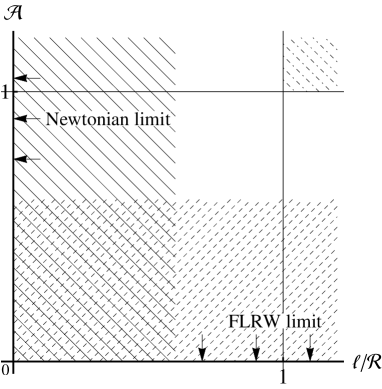
Figure 6: A schematic picture representing a relation between the analysis for perturbations developed in our previous paper and that in this paper, where $\mathcal{A}$, $\ell$ and $\mathcal{R}$ denote the amplitude of inhomogeneity of the background huge void model, the length scale of perturbations and the curvature radius of the background . The region shaded by dashed lines and the region shaded by solid lines represent domains in which the approximation schemes adopted in our previous work and in this paper, respectively.

In our previous works Nishikawa:2012we ; Nishikawa:2013rna , we studied the linear perturbations in the huge void universe model without any distinctions between relativistic and non-relativistic perturbations, by treating the background huge void as an isotropic perturbation in the background model of the homogeneous and isotropic universe filled with dust. By contrast, the method of analysis based on the tidal approximation is applicable, even if the background void structure is highly nonlinear. In Fig. 6, we have shown a schematic picture representing the relation between our two independent approaches. Here, $\mathcal{A}$ denotes the amplitude of radial inhomogeneities in the background huge void universe model, that is, the huge void itself, and $\ell/\mathcal{R}$ denotes the ratio of the length scale of perturbations to the spacetime curvature radius of the background which is assumed to be almost the same as the size of the void in the case of the huge void universe model. The region shaded by dashed lines in Fig. 6 represents the domain in which the approximation scheme adopted in our previous works Nishikawa:2012we ; Nishikawa:2013rna is applicable. The region shaded by solid lines in Fig. 6 represents the domain in which the approximation scheme adopted in the present paper is applicable. We can see that the region shaded by dot-dashed lines in Fig. 6 is the domain to which neither the approximation scheme adopted in our previous works nor that adopted in the present paper is applicable. The system included in this region is composed of relativistic perturbations in the highly non-linear huge void. The study of perturbations in this region seems to be difficult without invoking the numerical simulations, and we leave it for a future work.

References

- (1) P. Bull and T. Clifton, Phys. Rev. D 85, 103512 (2012).
- (2) M. N. Celerier, Astron. Astrophys. 353, 63 (2000).
- (3) M. N. Celerier, K. Bolejko and A. Krasinski, Astron. Astrophys. 518, A21 (2010).
- (4) T. Clifton, P. G. Ferreira and K. Land, Phys. Rev. Lett. 101, 131302 (2008).
- (5) S. P. Goodwin, P. A. Thomas, A. J. Barber, J. Gribbin and L. I. Onuora, arXiv:astro-ph/9906187.
- (6) H. Iguchi, T. Nakamura and K. i. Nakao, Prog. Theor. Phys. 108, 809 (2002).
- (7) E. W. Kolb and C. R. Lamb, arXiv:0911.3852 [astro-ph.CO].
- (8) N. Mustapha, C. Hellaby, G. F. R. Ellis, Mon. Not. Roy. Astron. Soc. 292, 817-830 (1997).
- (9) K. Tomita, Astrophys. J. 529, 38 (2000).
- (10) K. Tomita, Mon. Not. Roy. Astron. Soc. 326, 287 (2001).
- (11) K. Tomita, Prog. Theor. Phys. 106, 929 (2001).
- (12) R. A. Vanderveld, E. E. Flanagan and I. Wasserman, Phys. Rev. D 74, 023506 (2006).
- (13) C. M. Yoo, T. Kai and K. i. Nakao, Prog. Theor. Phys. 120, 937 (2008).
- (14) C. -M. Yoo, Prog. Theor. Phys. 124, 645-665 (2010).
- (15) S. Alexander, T. Biswas, A. Notari and D. Vaid, JCAP 0909, 025 (2009).
- (16) H. Alnes, M. Amarzguioui and O. Gron, Phys. Rev. D 73, 083519 (2006).
- (17) T. Biswas, A. Notari and W. Valkenburg, JCAP 1011, 030 (2010).
- (18) K. Bolejko and J. S. B. Wyithe, JCAP 0902, 020 (2009).
- (19) C. Clarkson and M. Regis, JCAP 1102, 013 (2011).
- (20) J. Garcia-Bellido and T. Haugboelle, JCAP 0804, 003 (2008).
- (21) V. Marra and A. Notari, Class. Quant. Grav. 28, 164004 (2011).
- (22) V. Marra and M. Paakkonen, JCAP 1012, 021 (2010).
- (23) A. Moss, J. P. Zibin and D. Scott, Phys. Rev. D 83, 103515 (2011).
- (24) S. Nadathur and S. Sarkar, Phys. Rev. D 83, 063506 (2011).
- (25) C. M. Yoo, K. i. Nakao and M. Sasaki, JCAP 1007, 012 (2010).
- (26) J. P. Zibin, A. Moss and D. Scott, Phys. Rev. Lett. 101, 251303 (2008).
- (27) J. Garcia-Bellido and T. Haugboelle, JCAP 0909, 028 (2009).
- (28) M. Zumalacarregui, J. Garcia-Bellido and P. Ruiz-Lapuente, JCAP 1210, 009 (2012).
- (29) P. Bull, T. Clifton and P. G. Ferreira, Phys. Rev. D 85, 024002 (2012).
- (30) J. Garcia-Bellido and T. Haugboelle, JCAP 0809, 016 (2008).
- (31) A. Moss and J. P. Zibin, Class. Quant. Grav. 28, 164005 (2011).
- (32) C. M. Yoo, K. i. Nakao and M. Sasaki, JCAP 1010, 011 (2010).
- (33) P. Zhang and A. Stebbins, Phys. Rev. Lett. 107, 041301 (2011).
- (34) P. A. R. Ade et al. [Planck Collaboration], Astron. Astrophys. 561, A97 (2014).
- (35) M. Adachi and M. Kasai, Prog. Theor. Phys. 127, 145 (2012).
- (36) H. Alnes and M. Amarzguioui, Phys. Rev. D 75, 023506 (2007).
- (37) K. Bolejko, M. -N. Celerier and A. Krasinski, Class. Quant. Grav. 28, 164002 (2011).
- (38) K. Bolejko, PMC Phys. A 2, 1 (2008).
- (39) R. R. Caldwell and N. A. Maksimova, Phys. Rev. D 88, no. 10, 103502 (2013).
- (40) M. -N. Celerier, arXiv:1203.2814 [astro-ph.CO].
- (41) C. Clarkson, Comptes Rendus Physique 13, 682 (2012).
- (42) R. de Putter, L. Verde and R. Jimenez, JCAP 1302, 047 (2013).
- (43) P. Dunsby, N. Goheer, B. Osano and J. P. Uzan, JCAP 1006, 017 (2010).
- (44) K. Enqvist, M. Mattsson and G. Rigopoulos, JCAP 0909, 022 (2009).
- (45) K. Enqvist and T. Mattsson, JCAP 0702, 019 (2007).
- (46) H. Goto and H. Kodama, Prog. Theor. Phys. 125, 815 (2011).
- (47) A. F. Heavens, R. Jimenez and R. Maartens, JCAP 1109, 035 (2011).
- (48) M. Quartin and L. Amendola, Phys. Rev. D 81, 043522 (2010).
- (49) M. Regis and C. Clarkson, Gen. Rel. Grav. 44, 567 (2012).
- (50) A. E. Romano, Phys. Rev. D 82, 123528 (2010).
- (51) A. E. Romano, M. Sasaki and A. A. Starobinsky, Eur. Phys. J. C72, 2242 (2012).
- (52) A. E. Romano and P. Chen, JCAP 1110, 016 (2011).
- (53) M. Tanimoto, Y. Nambu and K. Iwata, arXiv:0906.4857 [astro-ph.CO].
- (54) K. Tomita, arXiv:0906.1325 [astro-ph.CO].
- (55) K. Yagi, A. Nishizawa and C. -M. Yoo, J. Phys. Conf. Ser. 363, 012056 (2012).
- (56) J. P. Zibin, Phys. Rev. D 84, 123508 (2011).
- (57) W. Valkenburg, M. Kunz and V. Marra, Phys. Dark Univ. 2, 219 (2013).
- (58) W. Valkenburg, V. Marra and C. Clarkson, MNRAS 438, (2014) L6.
- (59) D. Alonso, J. Garcia-Bellido, T. Haugboelle and A. Knebe, Phys. Dark Univ. 1, 24 (2012).
- (60) D. Alonso, J. Garcia-Bellido, T. Haugbolle and J. Vicente, Phys. Rev. D 82, 123530 (2010).
- (61) C. Clarkson, T. Clifton and S. February, JCAP 0906, 025 (2009).
- (62) S. February, C. Clarkson and R. Maartens, JCAP 1303, 023 (2013).
- (63) S. February, J. Larena, C. Clarkson and D. Pollney, arXiv:1311.5241 [astro-ph.CO].
- (64) J. P. Zibin, Phys. Rev. D 78, 043504 (2008).
- (65) R. Nishikawa, C. -M. Yoo and K. -i. Nakao, Phys. Rev. D 85, 103511 (2012).
- (66) R. Nishikawa, C. -M. Yoo and K. -i. Nakao, Phys. Rev. D 88, 123520 (2013).
- (67) R. Nishikawa, K. i. Nakao and C. M. Yoo, arXiv:1407.4899 [astro-ph.CO].
- (68) P. J. E. Peebles, “The Large-Scale Structure of the Universe,” (Princeton University Press, Princeton, 1980).
- (69) T. Futamase, Mon. Not. Roy. Astron. Soc. 237, 187 (1989).
- (70) J. -C. Hwang, H. Noh and D. Puetzfeld, JCAP 0803, 010 (2008).
- (71) M. Shibata and H. Asada, Prog. Theor. Phys. 94, 11 (1995).
- (72) K. Tomita, Prog. Theor. Phys. 79, 2 (1988).
- (73) F.K. Manasse and C.W. Misner, J. Math. Phys. 4, 735 (1963).
- (74) M. Ishii, M. Shibata and Y. Mino, Phys. Rev. D 71, 044017 (2005).
- (75) T. Baldauf, U. Seljak, L. Senatore and M. Zaldarriaga, JCAP 1110, 031 (2011).
- (76) D. Klein and P. Collas, Class. Quant. Grav. 25, 145019 (2008).
- (77) E. Poisson, “A relativist’s toolkit,” (Cambridge University Press, Cambridge, 2004).
- (78) F. Schmidt and D. Jeong, Phys. Rev. D 86, 083513 (2012).
- (79) B. Mashhoon, N. Mobed and D. Singh, Class. Quant. Grav. 24, 5031 (2007).
- (80) R. M. Wald, “General Relativity,” (The University of Chicago Press, Chicago, 1984).
- (81) U.H. Gerlach and U.K. Sengupta, Phys. Rev. D 19, 2268 (1979).