Dust correction factors over $0<z<3$ in massive star-forming galaxies from stacking in Herschel

In this work we use stacking analysis in Herschel PACS to study the accuracy of several dust-correction factors typically employed to estimate total star-formation rate (SFR) of high-redshift star-forming (SF) galaxies. We also analyze what stacking suggests about the relation between SFR and stellar mass and the redshift evolution of the specific SFR (${\rm sSFR}={\rm SFR}/{\rm M_{*}}$). We find that the dust properties of massive SF galaxies evolve with redshift, being galaxies at $z\sim 2-3$ more attenuated than at $z\sim 1$ for a given UV continuum slope and stellar mass. As a consequence, a single IRX-$\beta$ relation can not be used to recover the total SFR of massive SF galaxies at $0\lesssim z\lesssim 3$. This might have implications for higher redshift studies, where a single IRX-$\beta$ relation derived for local starburst is usually assumed to be valid. However, we find that the local relation between dust attenuation and stellar mass is valid at least up to $z\sim 1$, although deviations are found for higher redshift galaxies where only $\log{\left(M_{*}/M_{\odot}\right)}>10.25-10.50$ galaxies are detected through stacking. This, therefore, does not rule out the possibility that the local dust-mass relation can be valid for less massive SF galaxies at $z\sim 2-3$. The SED fitting procedure with stellar population templates gives over-estimated values (about 0.3–0.5 dex in $\log{\rm SFR}$) of the dust-corrected SFR at all redshifts studied here. We find that the slope of the main-sequence of star formation is less steep than previously found in massive galaxies with $\log{\left(M_{*}/M_{\odot}\right)}\geq 10$, and the redshift evolution of the sSFR reported in previous works in massive is well recovered.

1 Introduction

In order to estimate dust attenuation and total SFRs of SF galaxies at different redshifts several recipes have been traditionally employed in the literature when FIR information is not available. These include the IRX-$\beta$ relation derived for local starburst (SB) (Meurer et al., 1999) or using properties derived using UV/optical/NIR SED fits that do not include FIR data. However, there is increasing evidence that the dust properties of massive SF galaxies might have evolved with redshift and that local relations cannot be applied to high-redshift or special kinds of galaxies (Goldader et al., 2002; Oteo et al., 2013b).

Most previous that analyze dust correction factors in SF galaxies are based on direct detection in Herschel (Pilbratt et al., 2010) bands (Buat et al., 2010; Wuyts et al., 2011; Oteo et al., 2014). In fact, the most accurate values of dust attenuation and total SFR are those derived with individual detections in the FIR. Unfortunately, for a given redshift slice, only a small fraction of galaxies those with the highest total SFRs can be individually detected by Herschel even in the deepest surveys (Magdis et al., 2010; Rigopoulou et al., 2010; Heinis et al., 2013; Oteo et al., 2013c, b, 2014). Furthermore, a significant population of the high-redshift galaxies detected by Herschel are starburst rather than normal SF galaxies (see for example Rodighiero et al., 2014). Therefore, if we want to study less extreme sources, we need to rely on stacking analysis. In this work we study the accuracy of several dust-correction factors (IRX-$\beta$ relation, dust-mass correlation, and SED fits) at different redshifts from stacking analysis in Herschel PACS-160 $\mu$m (Poglitsch et al., 2010). We also explore what stacking tells us about the relation between SFR and stellar mass in massive SF galaxies and about the redshift evolution of the specific SFR (${\rm sSFR}$). This paper is organized as follows: Section 2 explains the source selection and the methodology employed in this work. The main results are presented in Section 3. Finally, we summarize our main conclusions in Section 4. Throughout the paper, we assume a flat universe with $(\Omega_{m},\Omega_{\Lambda},h_{0})=(0.3,0.7,0.7)$, and all magnitudes are listed in the AB system (Oke & Gunn, 1983).

2 Source selection and methodology

We focus our work on the COSMOS field (Scoville et al., 2007) and select all the rest-frame UV-selected sources whose photometric redshifts (taken from Ilbert et al. (2013)) are within $0.02\leq z\leq 4.0$. We avoid AGN contamination by discarding all galaxies detected in X-rays (Elvis et al., 2009). In this work we are interested in SF galaxies. Different ways of selecting SF galaxies have been proposed in the literature, mostly based on single and double colors (Williams et al., 2009; Rodighiero et al., 2010). However, a single color cut might produce the loss of SF galaxies with red rest-frame $U-V$ colors (see figure 11 in Williams et al., 2009). Also, red SF galaxies might occupy the green valley of even the red sequence of galaxies (Oteo et al., 2014). Since SF galaxies are galaxies that form stars, we select SF galaxies basing on their SFR. In this way, we consider only galaxies whose ${\rm SFR_{UV}}$ (uncorrected from dust attenuation) is at least 1 $M_{\odot}\,{\rm yr}^{-1}$. This is a conservative approach, since a high percentage of low-redshift galaxies have SFR higher than that threshold (Elbaz et al., 2007), and SF galaxies with ${\rm SFR}\geq 1M_{\odot}\,{\rm yr}^{-1}$ can be detected at the highest redshifts studied in this work with the depth of the data we are using. We have also compared with results adopting a threshold ${\rm SFR_{UV}}\geq 5M_{\odot}\,{\rm yr}^{-1}$ at $z\geq 1$. Note that since the above limit is before any dust correction, the actual SFR would be even higher.

The UV-to-NIR SEDs are fitted with Bruzual & Charlot (2003) templates to obtain the stellar masses, UV continuum slope ($\beta$), and rest-frame UV luminosities ($L_{\rm UV}$) of our studied galaxies (see for example Oteo et al., 2013a). Optical and NIR photometric information is also taken from Ilbert et al. (2013), while GALEX data are taken from Zamojski et al. (2007) for galaxies at $z\leq 1$. In this step, Bruzual & Charlot (2003) templates associated to constant SFR and $Z=0.2Z_{\odot}$ metallicity are considered. Dust attenuation is included with the Calzetti et al. (2000) law. We also include intergalactic medium absorption adopting the prescription of Madau (1995). The SED fits are carried out with the Zurich Extragalactic Bayesian Redshift Analyzer (ZEBRA, Feldmann et al., 2006) code.

Since most of the galaxies are undetected by Herschel we must rely on an stacking analysis to estimate the FIR emission of UV-selected galaxies. To this aim we use the IAS stacking library (Béthermin et al., 2010) and focus on the PACS-160 $\mu$m band. We have checked that stacking in PACS-100 $\mu$m gives similar results (see also Rodighiero et al., 2010). We stack in the residual images and median stacked image are considered. It should be noted that only Herschel-undetected galaxies are considered in the stacking analysis. The stacked fluxes are obtained with a PSF-fitting procedure and their uncertainties are calculated with bootstrap. We studied the effect of clustering effect (Béthermin et al., 2012) by comparing the PSF of PACS-160 $\mu$m with the actual radial profile of each stacked detection. This is similar to the method used in Heinis et al. (2013) (see also Method C in Béthermin et al. 2012). Comparing the profile of the stacked detections and the profile of the PSF of the PACS-160 $\mu$m observations, we do not find additional broadening of the stacked emission due to clustering of the input catalog and, consequently, we do not include any extra correction (Magnelli et al., 2014). Radial profiles and stacked images are shown in Appendix A for stacks as a function of the UV continuum slope and stellar mass (see later in the text). The PACS-160 $\mu$m are converted to total IR luminosities ($L_{\rm IR}$) with single band extrapolations using the Chary & Elbaz (2001) templates. This step provides good estimation of $L_{\rm IR}$ since PACS-160 $\mu$m samples the dust emission peak at the redshift range of the galaxies studied. The stacked total SFR are obtained from luminosities with the Kennicutt (1998) relations and adopting ${\rm SFR_{total}}={\rm SFR_{UV}}+{\rm SFR_{IR}}$. Dust attenuation is obtained from the ratio between $L_{\rm IR}$ and $L_{\rm UV}$ luminosities assuming the Buat et al. (2005) calibration. We will stack as a function of UV continuum slope, stellar mass, and dust attenuation. We only consider in this study stacked detections with $f_{\rm stack}\geq 3\sigma_{\rm stack}$, where $\sigma_{\rm stack}$ is the uncertainty in each stacked flux. With the PACS data used in this work, stacked detection are only recovered for massive galaxies, typically with $\log{\left(M_{*}/M_{\odot}\right)}\gtrsim 10$. Therefore, we will only deal with a massive population os SF galaxies. Furthermore, despite we consider galaxies up to $z\sim 4$, we only recover stacked detections for galaxies at $z\leq 3$. Tables 1 and 2 summarize the stacked fluxes, rest-frame UV and total IR luminosities, and number of sources in each redshift and UV slope bin for the stacked detection as a function of UV continuum slope and stellar mass. It should be noted that we do not employ individual detections in our study since with the depth of Herschel observations in COSMOS, only the most-extreme sources are detected, and they might not be normal SF galaxies, but likely have a SB nature. In any case, the detection rate in Herschel bands is low and this does not change the main conclusions of our work.

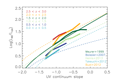
Figure 1: Relation between the total IR and rest-frame UV luminosities (a proxy for dust attenuation) agains the UV continuum slope as seen by our stacking analysis over $0.02\lesssim z\lesssim 3.0$, with the color-code shown in the top-left legend. We also represent the IRX-$\beta$ relations reported in previous works (Meurer et al., 1999; Boissier et al., 2007; Heinis et al., 2013; Takeuchi et al., 2012; Buat et al., 2012), as indicated in the bottom-right legend. Their color code is related to the data they fits best to.

3 Results

Figure 1 shows the relation between dust attenuation (parametrized by the $L_{\rm IR}/L_{\rm UV}$ ratio) against the UV continuum slope for our SF galaxies at different redshifts. As expected, redder galaxies are more attenuated. There is a clear trend with redshift for galaxies with $\beta\geq-1.0$: for a given UV continuum slope, galaxies at $z\sim 2-3$ are more attenuated than those at $z\sim 1$. This result is similar to the ones found for individual detections in PACS/SPIRE (Oteo et al., 2013b, c, 2014), but now with a staking analysis and, therefore, being able to probe less dusty and IR-fainter galaxies at each epoch. At $z\lesssim 1$, where we can detect bluer galaxies, dust attenuation has not significantly changed with redshift for $\beta<-1.0$ SF galaxies. This might indicate that dust attenuation evolved only in massive, red SF galaxies, although deeper data would be needed to confirm this.

These results confirm the evolution of the dust properties of massive galaxies over $0<z<3$. As a consequence of this evolutionary trend, there is not a single IRX-$\beta$ relation that can be applied at all redshifts to accurately recover the dust attenuation or total SFR in massive SF galaxies. At low redshift, stacked points are in agreement with the Takeuchi et al. (2012) relation, but the Buat et al. (2012) relation should be applied at $z\sim 2-3$, where galaxies were more attenuation for a given UV continuum slope. We recall that at $z\sim 1.5$ our stacked points are in great agreement with the Heinis et al. (2013) relation, that was obtained with galaxies around that redshift through stacking in SPIRE bands.

As shown in Figure 1, even with stacking analysis in Herschel, we do not recover stacked detections for galaxies with $\beta\lesssim-1.5$ at any redshift (see also Heinis et al., 2013), nor with $\beta<-1.1$ at $z\geq 1.5$. This represents a problem for testing the accuracy of the IRX-$\beta$ relations at recovering dust attenuation. This is because the SF galaxies selected in UV, optical, or NIR surveys have actually UV continuum slopes $\beta\lesssim-1.25$ in most cases (Oteo et al., 2013b, a, 2014). Therefore, applying a single IRX-$\beta$ relation should be done with care, because it has been shown here to evolve with redshift for massive, red ($\beta\geq-1.1$) SF galaxies but we do not know its behavior at lower masses and bluer UV slopes at different redshifts.

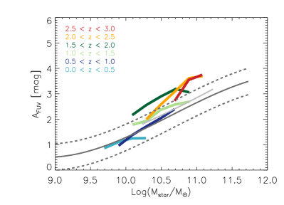
Figure 2: Relation between dust attenuation and stellar mass for our stacked galaxies over $0.02\lesssim z\lesssim 3.0$, with the color-code shown in the top-left legend. Dust attenuation has been derived with the $L_{\rm IR}/L_{\rm UV}$ ratio and the Buat et al. (2005) calibration. For a reference, we represent the local relation as reported in Sobral et al. (2012) with a solid dark grey curve and the relation at $z\sim 1.5$ presented in Heinis et al. (2014) with a light grey solid line.

Figure 2 represents the dust attenuation in the FUV band (rest-frame 1500 Å) as a function of stellar mass for our SF galaxies at different redshifts. More massive galaxies are more attenuated, as obtained in several previous works (Ibar et al., 2013; Garn & Best, 2010; Heinis et al., 2014). A trend with redshift is also present, being massive ($\log{\left(M_{*}/M_{\odot}\right)}\geq 10$) galaxies at $z\sim 2-3$ more attenuated for a given stellar mass than at $z\lesssim 1$. The Heinis et al. (2014) is well recovered at their same redshift, $z\sim 1.5$. Since only galaxies with $\log{\left(M_{*}/M_{\odot}\right)}\geq 10$ have stacked detections at $z\geq 1$, we can only confirm the evolution in that mass range. At lower redshift, where we can detect less massive galaxies, we find that the relation between dust attenuation and stellar mass is in very good agreement to the one found for local galaxies (Garn & Best, 2010). This might indicate that, as it might occur for blue galaxies, the dust attenuation in less massive galaxies does not change significantly with redshift. This is what it was actually obtained in Sobral et al. (2012) for H$\alpha$ emitters at $z\sim 1.47$ and also with stacking analysis in HAEs at the same redshift in Ibar et al. (2013). This result would be quite important for recovering the dust attenuation or total SFR in $\log{\left(M_{*}/M_{\odot}\right)}\lesssim 10$ SF galaxies when FIR information is not available.

The power of the SED fitting method for recovering the total SFR in massive galaxies is shown in Figure 3. It can be seen that, at any redshift, the SED-derived total SFR is systematically higher than those obtained from stacking analysis. The over-estimation is about 0.3–0.5 dex at all redshifts, despite a little bit higher for the galaxies with the highest SED-derived SFRs. At high redshift and for FIR-bright galaxies individually detected with PACS, the SED-derived total SFR is an under-estimation of the much more accurate SFR derived with direct UV and IR data (Wuyts et al., 2011; Oteo et al., 2013b). However, the stacking analysis presented here indicates that the SED-fitting method actually over-estimates the total SFR at $0<z<3$ when galaxies with lower $L_{\rm IR}$ can be studied.

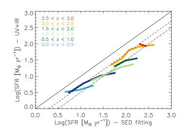
Figure 3: Relation between the dust-corrected total SFRs derived with stacking analysis in PACS and from a SED fitting method assuming a constant SFR and fixed metallicity $Z=0.2Z_{\odot}$. The one-to-one relation is shown with a black solid line, whereas deviations of -0.3 and -0.5 dex are indicated with dashed and dotted-dashed lines, respectively.

The relation between SFR and stellar mass for our stacked massive galaxies is shown in Figure 4. Most previous works agree that there is a relation between SFR and stellar mass for normal SF galaxies, the so-called main sequence (MS, Daddi et al., 2007; Elbaz et al., 2007). Despite there are many evidence that the MS exists, there is no consensus about its slope at different redshifts. This is mainly due to the different methods that can be employed to derive the stellar mass and total SFR of SF galaxies. Our stacking analysis reveals that the slope of the MS for massive ($\log{\left(M_{*}/M_{\odot}\right)}\geq 10$) SF galaxies is less stepper than previously reported (Elbaz et al., 2007; Daddi et al., 2007), mainly at our highest redshifts. We cannot detect less massive galaxies with stacking under the depths of the PACS images used here. Thus, it might be possible that there is a break of the MS in massive galaxies, being the slope steeper for galaxies with lower stellar masses and less steep for the most massive galaxies at each redshift. Deeper FIR data would be needed to confirm this. The results shown in Heinis et al. (2014) also indicate that the slope of the MS might be lower for massive galaxies. They fit a linear relation to their points, although the points tend to follow the Daddi et al. (2007) relation for their lowest massive galaxies and then they flattens at higher stellar masses. This flattening would be in agreement with a break in the SFR-mass relation and it is consistent with our results at the same redshift and over the same stellar mass range. At $z\sim 1$, our results are in agreement with Rodighiero et al. (2010). At higher redshifts, Rodighiero et al. (2010) obtained higher slopes although their galaxies are selected by having a blue optical color and therefore might be biased towards bluer galaxies than those studied here, that cover a wider range of optical colors. It might be argued that the flattening of the MS at the highest redshifts is due to the presence of quiescent galaxies. Despite we have selected our galaxies for being SF due to their SFR, we have repeated the stacking when increasing the ${\rm SFR_{UV}}$ threshold to 5 $M_{\odot}\,{\rm yr}^{-1}$ for galaxies at $z\geq 1$ (again, before any dust correction, being the real SFR even higher) to include only more active SF galaxies. It can be seen in Figure 4 that even for these more active SF galaxies the slope of the MS is lower than previously reported, suggesting that the flattening of the MS in massive galaxies is not due to the presence of quiescent galaxies.

The redshift evolution of the specific SFR (${\rm sSFR}={\rm SFR}/{\rm M_{\odot}}$) determined through stacking is in agreement with previous compilations obtained with different methodologies, increasing about one order of magnitude between $z\sim 0$ and $z\sim 2$. This is shown in the inset plot of Figure 4 where we compare the sSFR obtained with stacking with the Dutton et al. (2010) compilation at the same redshift range for galaxies with $\log{\left(M_{*}/M_{\odot}\right)}\sim 10.5$.

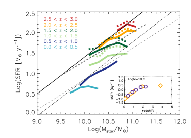
Figure 4: Relation between ${\rm SFR}={\rm SFR_{UV}}+{SFR_{IR}}$ and stellar mass for massive galaxies as revealed by our stacking analysis. We represent with dashed curves the points when the ${\rm SFR_{UV}}$ is limited to values higher than 5 $M_{\odot}\,{\rm yr}^{-1}$. The Elbaz et al. (2007) (black dotted-dashed line), Daddi et al. (2007) (black solid line), and Heinis et al. (2014) (thick grey dashed line) MS are included. We also show the MS with a slope of 0.75 and the same normalization of Daddi et al. (2007) to reflect the Rodighiero et al. (2010) results at $z\leq 1$. We show in the bottom-right inset plot the evolution of the ${sSFR}={SFR}/{M_{*}}$ for galaxies with $\log{\left(M_{*}/M_{\odot}\right)}\sim 10.5$. We also include the Dutton et al. (2010) compilation with orange open squares.

4 Conclusions

By using a stacking analysis in Herschel bands, we have studied the accuracy of several dust-correction factors traditionally employed to recover the total SFR of high-redshift star-forming (SF) galaxies. Our main conclusions are:

1. We find that the dust attenuation in massive ($\log{\left(M_{*}/M_{\odot}\right)}>10$) SF galaxies is higher at $z\sim 2-3$ than at $z\sim 1$ for a given UV continuum slope and stellar mass. This is consistent what it was previously found with individual Herschel detections. At $z\lesssim 1$, where stacking is able to detected less massive, we do not find significant evolution of dust attenuation for a given stellar mass with respect to galaxies in the local universe.

2. There is not a single IRX-$\beta$ relation that can be applied to accurately recover the dust attenuation or total SFR of massive SF galaxies at any redshifts. Low-redshift galaxies are better parametrized by the Takeuchi et al. (2012) IRX-$\beta$ relation, but the Buat et al. (2012) one is more appropriate at $z\sim 2$, when dust attenuation was higher for a given UV slope. This might have implications in high-redshift studies, where a single IRX-$\beta$ relation is normally assumed to correct for dust attenuation. The SED-derived dust attenuation gives over-estimated total SFRs at all redshifts studied here.

3. Despite the dust attenuation of massive galaxies is higher at $z\sim 2-3$ than at $z\sim 1$, our stacking analysis indicates that the local relation between dust attenuation and stellar mass is valid up to $z\sim 1$. Since we do not recover stacked detections at $z\geq 1.5$ for $\log{\left(M_{*}/M_{\odot}\right)}\lesssim 10$ galaxies we cannot confirm the non evolution of the local dust-mass relation in low-mass galaxies at higher redshift reported in previous works.

4. We obtain that the slope of the MS of massive SF galaxies is lower than previously reported. Since we do not recover stacked detection for galaxies with $\log{\left(M_{*}/M_{\odot}\right)}\lesssim 10$, we cannot distinguish if this is also true for less massive galaxies or there is a break in the MS for massive galaxies. The redshift evolution of the sSFR is in agreement with previous findings, increasing in about one order of magnitude from $z\sim 0.02$ to $z\sim 2$.

Appendix A Additional plots and table

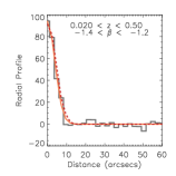
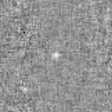
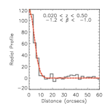
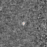
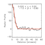
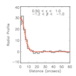
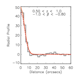
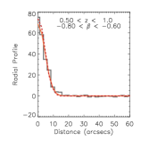
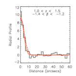
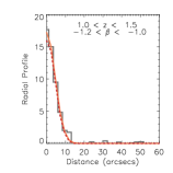
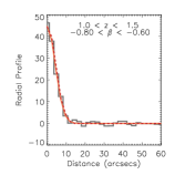
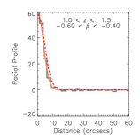
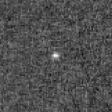
Figure 5: Radial profiles and associated stacked images when stacking as a function of the UV continuum slope. Redshift and UV continuum bins are indicated in each case. Orange curves are the best-fitted gaussian to the radial profile, while red dashed curves represent the shape of the PACS-160 $\mu$m PSF.

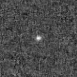
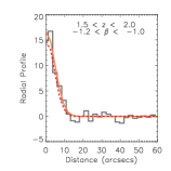
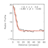
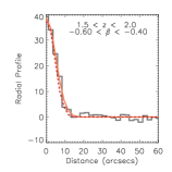
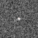
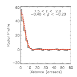
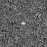
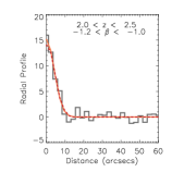
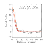
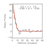
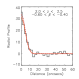
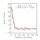
Figure 6: Radial profiles and associated stacked images when stacking as a function of the UV continuum slope. Redshift and UV continuum bins are indicated in each case (Cont) .

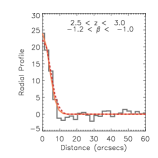
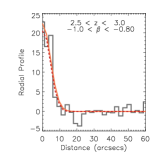
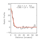
Figure 7: Radial profiles and associated stacked images when stacking as a function of the UV continuum slope. Redshift and UV continuum bins are indicated in each case (Cont).

Table 1: Summary of stacked properties when stacking as a function of the UV continuum slope. The uncertainties in the rest-frame UV luminosity are related to the normalization of the templates to the observed photometry and they are typically lower tan 0.05 dex. The uncertainties in the total IR luminosities are obtained as the difference in the total IR luminosity when considering $f_{\rm 160\mu m}\pm\Delta f_{\rm 160\mu m}$. $N$ indicates the number of galaxies in each bin.

Redshift range	UV slope range	$f_{\rm 160\mu m}$ [mJy]	$\log{L_{\rm UV}}$	$\log{L_{\rm IR}}$	$N$
0.02$\leq z\leq$0.5	-1.4$\leq\beta\leq$-1.2	1.77$\pm$0.19	9.61	9.98$\pm$0.09	194
0.02$\leq z\leq$0.5	-1.2$\leq\beta\leq$-1.0	2.73$\pm$0.29	9.61	10.16$\pm$0.09	121
0.02$\leq z\leq$0.5	-1.0$\leq\beta\leq$-0.8	3.25$\pm$0.46	9.58	10.34$\pm$0.17	41
0.5$\leq z\leq$1.0	-1.4$\leq\beta\leq$-1.2	0.49$\pm$0.04	9.72	10.22$\pm$0.07	3125
0.5 $\leq z\leq$1.0	-1.2$\leq\beta\leq$-1.0	0.82$\pm$0.06	9.72	10.44$\pm$0.06	2064
0.5$\leq z\leq$1.0	-1.0$\leq\beta\leq$-0.8	1.18$\pm$0.08	9.73	10.60$\pm$0.05	1244
0.5$\leq z\leq$1.0	-0.8$\leq\beta\leq$-0.6	1.59$\pm$0.10	9.70	10.72$\pm$0.05	963
1.0$\leq z\leq$1.5	-1.4$\leq\beta\leq$-1.2	0.18$\pm$0.02	9.86	10.28$\pm$0.09	8136
1.0$\leq z\leq$1.5	-1.2$\leq\beta\leq$-1.0	0.41$\pm$0.03	9.84	10.61$\pm$0.06	5084
1.0$\leq z\leq$1.5	-1.0$\leq\beta\leq$-0.8	0.65$\pm$0.03	9.84	10.81$\pm$0.04	4187
1.0$\leq z\leq$1.5	-0.8$\leq\beta\leq$-0.6	0.97$\pm$0.05	9.81	10.98$\pm$0.05	2634
1.0$\leq z\leq$1.5	-0.6$\leq\beta\leq$-0.4	1.16$\pm$0.06	9.80	11.05$\pm$0.04	1628
1.0$\leq z\leq$1.5	-0.4$\leq\beta\leq$-0.2	1.54$\pm$0.07	9.74	11.15$\pm$0.04	1299
1.5$\leq z\leq$2.0	-1.2$\leq\beta\leq$-1.0	0.42$\pm$0.03	9.98	10.92$\pm$0.05	4359
1.5$\leq z\leq$2.0	-1.0$\leq\beta\leq$-0.8	0.56$\pm$0.04	9.95	11.05$\pm$0.06	3662
1.5$\leq z\leq$2.0	-0.8$\leq\beta\leq$-0.6	0.77$\pm$0.04	9.88	11.18$\pm$0.05	2501
1.5$\leq z\leq$2.0	-0.6$\leq\beta\leq$-0.4	1.01$\pm$0.06	9.83	11.31$\pm$0.05	1691
1.5$\leq z\leq$2.0	-0.4$\leq\beta\leq$-0.2	1.08$\pm$0.09	9.77	11.34$\pm$0.07	1061
1.5$\leq z\leq$2.0	-0.2$\leq\beta\leq$-0.0	1.11$\pm$0.09	9.76	11.33$\pm$0.06	825
2.0$\leq z\leq$2.5	-1.2$\leq\beta\leq$-1.0	0.31$\pm$0.05	10.21	11.13$\pm$0.15	2041
2.0$\leq z\leq$2.5	-1.0$\leq\beta\leq$-0.8	0.62$\pm$0.06	10.13	11.43$\pm$0.09	1470
2.0$\leq z\leq$2.5	-0.8$\leq\beta\leq$-0.6	0.82$\pm$0.09	10.07	11.53$\pm$0.10	857
2.0$\leq z\leq$2.5	-0.6$\leq\beta\leq$-0.4	0.73$\pm$0.09	9.91	11.49$\pm$0.10	776
2.0$\leq z\leq$2.5	-0.4$\leq\beta\leq$-0.2	1.14$\pm$0.12	9.86	11.69$\pm$0.08	526
2.5$\leq z\leq$3.0	-1.2$\leq\beta\leq$-1.0	0.47$\pm$0.07	10.40	11.56$\pm$0.15	1001
2.5$\leq z\leq$3.0	-1.0$\leq\beta\leq$-0.8	0.58$\pm$0.08	10.32	11.67$\pm$0.13	721
2.5$\leq z\leq$3.0	-0.8$\leq\beta\leq$-0.6	0.63$\pm$0.13	10.22	11.69$\pm$0.19	376

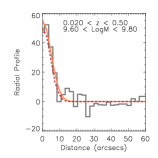
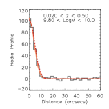
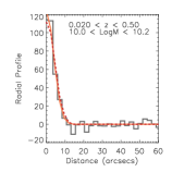
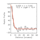
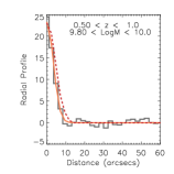
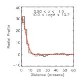
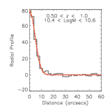
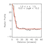
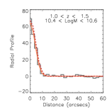
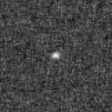
Figure 8: Radial profiles and associated stacked images when stacking as a function of the stellar mass. Redshift and stellar mass bins are indicated in each case. Orange curves are the best-fitted gaussian to the radial profile, while red dashed curves represent the shape of the PACS-160 $\mu$m PSF.

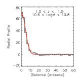
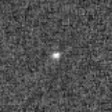
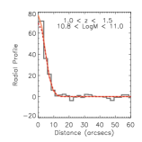
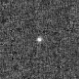
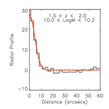
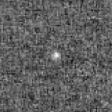
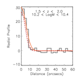
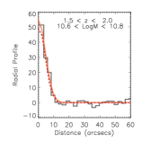
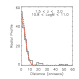
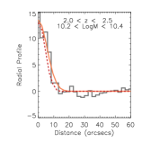
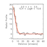
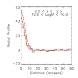
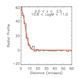
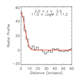
Figure 9: Radial profiles and associated stacked images when stacking as a function of the stellar mass. Redshift and stellar mass bins are indicated in each case. Orange curves are the best-fitted gaussian to the radial profile, while red dashed curves represent the shape of the PACS-160 $\mu$m PSF (Cont).

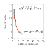
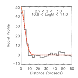
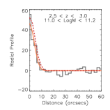
Figure 10: Radial profiles and associated stacked images when stacking as a function of the stellar mass. Redshift and stellar mass bins are indicated in each case. Orange curves are the best-fitted gaussian to the radial profile, while red dashed curves represent the shape of the PACS-160 $\mu$m PSF (Cont).

Table 2: Summary of stacked properties when stacking as a function of stellar mass. The uncertainties in the rest-frame UV luminosity are related to the normalization of the templates to the observed photometry and they are typically lower tan 0.05 dex. The uncertainties in the total IR luminosities are obtained as the difference in the total IR luminosity when considering $f_{\rm 160\mu m}\pm\Delta f_{\rm 160\mu m}$. $N$ indicates the number of galaxies in each bin.

Redshift range	Stellar mass range	$f_{\rm 160\mu m}$ [mJy]	$\log{L_{\rm UV}}$	$\log{L_{\rm IR}}$	$N$
0.02$\leq z\leq$0.50	9.60$\leq\log{\left(M_{*}/M_{\odot}\right)}\leq$ 9.80	1.39$\pm$0.16	9.64	9.90$\pm$0.10	184
0.02$\leq z\leq$0.50	9.80$\leq\log{\left(M_{*}/M_{\odot}\right)}\leq$ 10.00	2.18$\pm$0.23	9.69	10.12$\pm$0.09	170
0.02$\leq z\leq$0.50	10.00$\leq\log{\left(M_{*}/M_{\odot}\right)}\leq$10.20	2.55$\pm$0.23	9.67	10.19$\pm$0.07	111
0.02$\leq z\leq$0.50	10.20$\leq\log{\left(M_{*}/M_{\odot}\right)}\leq$10.40	2.34$\pm$0.46	9.64	10.11$\pm$0.17	36
0.50$\leq z\leq$1.00	9.80$\leq\log{\left(M_{*}/M_{\odot}\right)}\leq$ 10.00	0.42$\pm$0.04	9.78	10.13$\pm$0.10	2896
0.50$\leq z\leq$1.00	10.00$\leq\log{\left(M_{*}/M_{\odot}\right)}\leq$10.20	0.83$\pm$0.05	9.83	10.46$\pm$0.05	2246
0.50$\leq z\leq$1.00	10.20$\leq\log{\left(M_{*}/M_{\odot}\right)}\leq$10.40	1.30$\pm$0.06	9.82	10.64$\pm$0.04	1499
0.50$\leq z\leq$1.00	10.40$\leq\log{\left(M_{*}/M_{\odot}\right)}\leq$10.60	1.85$\pm$0.09	9.79	10.79$\pm$0.05	865
0.50$\leq z\leq$1.00	10.60$\leq\log{\left(M_{*}/M_{\odot}\right)}\leq$10.80	2.38$\pm$0.11	9.77	10.98$\pm$0.04	576
1.00$\leq z\leq$1.50	10.00$\leq\log{\left(M_{*}/M_{\odot}\right)}\leq$10.20	0.70$\pm$0.04	9.95	10.81$\pm$0.05	2877
1.00$\leq z\leq$1.50	10.20$\leq\log{\left(M_{*}/M_{\odot}\right)}\leq$10.40	0.90$\pm$0.05	9.97	10.90$\pm$0.04	2101
1.00$\leq z\leq$1.50	10.40$\leq\log{\left(M_{*}/M_{\odot}\right)}\leq$10.60	1.41$\pm$0.06	9.93	11.10$\pm$0.03	1541
1.00$\leq z\leq$1.50	10.60$\leq\log{\left(M_{*}/M_{\odot}\right)}\leq$10.80	1.64$\pm$0.10	9.87	11.15$\pm$0.05	1152
1.00$\leq z\leq$1.50	10.80$\leq\log{\left(M_{*}/M_{\odot}\right)}\leq$11.00	1.71$\pm$0.10	9.83	11.18$\pm$0.05	869
1.50$\leq z\leq$2.00	10.00$\leq\log{\left(M_{*}/M_{\odot}\right)}\leq$10.20	0.62$\pm$0.05	10.04	11.11$\pm$0.06	2688
1.50$\leq z\leq$2.00	10.20$\leq\log{\left(M_{*}/M_{\odot}\right)}\leq$10.40	0.85$\pm$0.06	9.98	11.25$\pm$0.06	1682
1.50$\leq z\leq$2.00	10.40$\leq\log{\left(M_{*}/M_{\odot}\right)}\leq$10.60	1.13$\pm$0.08	9.93	11.37$\pm$0.06	1158
1.50$\leq z\leq$2.00	10.60$\leq\log{\left(M_{*}/M_{\odot}\right)}\leq$10.80	1.33$\pm$0.10	9.89	11.46$\pm$0.06	851
1.50$\leq z\leq$2.00	10.80$\leq\log{\left(M_{*}/M_{\odot}\right)}\leq$11.00	1.08$\pm$0.12	9.83	11.35$\pm$0.09	656
2.00$\leq z\leq$2.50	10.20$\leq\log{\left(M_{*}/M_{\odot}\right)}\leq$10.40	0.40$\pm$0.05	10.27	11.26$\pm$0.12	2083
2.00$\leq z\leq$2.50	10.40$\leq\log{\left(M_{*}/M_{\odot}\right)}\leq$10.60	0.70$\pm$0.07	10.21	11.50$\pm$0.09	1514
2.00$\leq z\leq$2.50	10.60$\leq\log{\left(M_{*}/M_{\odot}\right)}\leq$10.80	0.90$\pm$0.08	10.06	11.60$\pm$0.07	984
2.00$\leq z\leq$2.50	10.80$\leq\log{\left(M_{*}/M_{\odot}\right)}\leq$11.00	1.32$\pm$0.12	9.976	11.76$\pm$0.07	616
2.00$\leq z\leq$2.50	11.00$\leq\log{\left(M_{*}/M_{\odot}\right)}\leq$ 11.20	1.30$\pm$0.15	9.90	11.76$\pm$0.09	389
2.50$\leq z\leq$3.00	10.60$\leq\log{\left(M_{*}/M_{\odot}\right)}\leq$10.80	0.69$\pm$0.10	10.38	11.75$\pm$0.12	645
2.50$\leq z\leq$3.00	10.80$\leq\log{\left(M_{*}/M_{\odot}\right)}\leq$11.00	1.05$\pm$0.13	10.16	11.93$\pm$0.11	418
2.50$\leq z\leq$3.00	11.00$\leq\log{\left(M_{*}/M_{\odot}\right)}\leq$11.20	0.90$\pm$0.17	10.04	11.87$\pm$0.16	197