Abstract

We examine spontaneous symmetry breaking of a renormalisable $U(1)\times U(1)$ gauge theory coupled to fermions when kinetic mixing is present. We do not assume that the kinetic mixing parameter is small. A rotation plus scaling is used to remove the mixing and put the gauge kinetic terms in the canonical form. Fermion currents are also rotated in a non-orthogonal way by this basis transformation. Through suitable redefinitions the interaction is cast into a diagonal form. This framework, where mixing is absent, is used for subsequent analysis. The symmetry breaking determines the fermionic current which couples to the massless gauge boson. The strength of this coupling as well as the couplings of the massive gauge boson are extracted. This formulation is used to consider a gauged model for dark matter by identifying the massless gauge boson with the photon and the massive state to its dark counterpart. Matching the coupling of the residual symmetry with that of the photon sets a lower bound on the kinetic mixing parameter. We present analytical formulae of the couplings of the dark photon in this model and indicate some physics consequences.

Key Words:  Kinetic mixing, Dark Matter

I Introduction

In a non-abelian gauge theory the field tensor $F_{\mu\nu}^{a}$ is gauge covariant and the kinetic term is ${\cal L}=-\frac{1}{4}F^{a\mu\nu}F_{\mu\nu}^{a}$, where $\mu,\nu$ are Lorentz indices and $a$ is a gauge index both of which are summed over. This form is determined by Lorentz and gauge invariance. For a $U(1)$ gauge theory, on the other hand, $F^{\mu\nu}$ by itself is gauge invariant. Therefore, if there are several $U^{i}(1)~{}(i=1,\ldots n)$ factors in a theory the possibility of mixed terms in the Lagrangian of the form $-\alpha_{ij}F^{i\mu\nu}F_{\mu\nu}^{j}~{}(i\neq j)$, where $\alpha_{ij}$ quantify the mixing (in a given basis), opens up. Indeed, such kinetic mixing has been noted in the literature [1] and its origin, especially in the context of grand unification where two $U(1)$ factors are often encountered, examined [2]. If both the $U(1)$ are embedded in a grand unified theory (GUT) such as $E_{6}$ then at the unification scale the mixing will vanish but it could be generated at low energy where the GUT symmetry is not exact, by renormalisation group (RG) effects. Phenomenological applications in the context of dark matter have considered the kinetic mixing of a “dark sector” $U(1)$ gauge field with the $U(1)_{Y}$ of the standard model [3]. The detectability of a such a dark photon in a number of experiments using different approaches has been examined [4]. The alternative of the kinetic mixing of the “dark sector” $U(1)$ with $U(1)_{EM}$ has also been proposed [5]. Possible tests of such a photon-dark photon mixing scenario are available in the literature [6]. Consequences of mixing between several dark sector $U(1)$ factors have been illustrated in [7].

In this work our endeavour has been to take a detailed look at the effect of spontaneous symmetry breaking on a theory with two kinetically mixed $U(1)$ factors where the gauge bosons also couple to fermions, that is, when interaction terms are present. In the literature such models are usually analysed with the assumption that the coefficient of the mixing term, $c$, is small. We have not imposed this restriction. On the contrary, we show that depending on the two $U(1)$ gauge coupling strengths, $g_{1}$ and $g_{2}$, a lower bound on the magnitude of $c$ will exist if the coupling of the final unbroken gauge symmetry is to match that of electromagnetism, $e$. In particular, we show that in this case $c$ must satisfy

$$\frac{1}{4}\left|\frac{g^{2}_{1}+g^{2}_{2}}{2e^{2}}-1\right|\leq|c|\leq\frac{1}{4}\;.$$ (1)

In the special case $g_{1}=g_{2}=e$ the lower bound on $c$ becomes zero. Also, if $(g_{1}^{2}+g_{2}^{2})>4e^{2}$ then there is no solution.

In general the presence of two $U(1)$ symmetries will entail all particles to carry two distinct charges. Consequently there are two fermionic currents. These currents couple exclusively to the two gauge bosons of the theory without any cross terms. In this way the starting basis of our analysis is defined.

We proceed in the following stages. In the first the mixing term $F^{1}_{\mu\nu}F^{2\mu\nu}$ is removed by a transformation of gauge bosons involving an orthogonal rotation and a scaling. The initial basis where kinetic mixing terms are present is denoted as the $A$ basis and the second where non-diagonal terms are removed as the $B$ basis. Thereafter spontaneous symmetry breaking of the type, $U^{1}(1)\times U^{2}(1)\rightarrow U^{3}(1)$ takes place. This causes a further orthogonal rotation of gauge bosons taking the $B$ basis to the mass eigenstates which we term as the $X$ basis. One of the states, $X^{1}_{\mu}$, associated with the unbroken $U^{3}(1)$ remains massless while the other state $X^{2}_{\mu}$ is massive. These mass eigenstates form an orthonormal basis. The original $A$ basis where mixing terms are present and which is related to this mass basis $X$ by orthogonal and scaling transformations cannot then be orthogonal. That leads us to no conflict as we can define charges of fermions and scalars consistently in the $B$ basis which is orthogonal.

We evaluate the couplings of the massless and massive gauge boson states to fermions after symmetry breaking. The massless eigenstate, $X^{1}_{\mu}$, couples to one particular combination of the two fermion currents. We express this specific combination in terms of the direction of symmetry breaking in the $U^{1}(1)\times U^{2}(1)$ space and further determine the coupling strength of the massless boson to the current related to the unbroken charge. The coupling of the massive gauge boson, $X^{2}_{\mu}$, is conveniently given in terms of the above current combination and another current which is orthogonal to it. We observe that the coupling of $X^{2}_{\mu}$ to the unbroken combination is controlled by the kinetic mixing parameter $c$.

We have indicated how these results on couplings may offer a window on the physics of Dark Matter via a calculable ordinary matter-dark matter interaction strength. We have given two examples. In the first, ordinary matter does not have any dark charges and also, as expected, the dark matter does not have electric charge. In the second example, an extra $U(1)$ of the dark sector is kinetically mixed with normal $U(1)_{EM}$. Spontaneous symmetry breaking occurs in such a manner that the unbroken direction remains along $U(1)_{EM}$. This means that only the dark $U(1)$ is broken. In such an event due to the presence of kinetic mixing in the unbroken theory we derive relations between gauge couplings in the broken theory. Such relations will not exist if kinetic mixing is absent.

Our paper is arranged as follows. In the next section we set up the notation and the transformation from the $A$- (mixed) to the $B$- (unmixed) basis. Symmetry breaking is considered in the following section and the $X$-basis is defined as the (orthogonal) mass basis for gauge bosons. Analytic expressions for the couplings of the gauge boson mass eigenstates to fermions are given in the next section. Possible application of these ideas in the context of dark matter are then considered. We end with our conclusions.

II Removing kinetic mixing by rotation and scaling

In general, the kinetic terms for a gauge theory consisting of two $U(1)$ groups can be written as

$${\cal L}_{gauge}=-\frac{1}{4}~{}F^{1}_{\mu\nu}F^{1~{}\mu\nu}-\frac{1}{4}~{}F^{2}_{\mu\nu}F^{2~{}\mu\nu}-2c~{}F^{1}_{\mu\nu}F^{2~{}\mu\nu}\;.$$ (2)

Here the field strengths are expressed in terms of gauge fields by the usual formula

$$F^{r}_{\mu\nu}=\partial_{\mu}A^{r}_{\nu}-\partial_{\nu}A^{r}_{\mu},~{}~{}~{}~{}{\rm where}~{}~{}r=1,2,$$ (3)

and $c$ is a real kinetic mixing parameter. Gauge invariance cannot fix the magnitude of $c$. In fact $c$ has different values for different basis choices. Once we are able to fix the basis $A^{1}_{\mu},A^{2}_{\mu}$ using a set of physical arguments, then $c$ becomes a meaningful parameter. The Lagrangian for the interaction of fermions with gauge bosons is

$${\cal L}_{int}=g_{1}j^{\mu}_{1}A^{1}_{\mu}+g_{2}j^{\mu}_{2}A^{2}_{\mu}=\pmatrix{j^{\mu}_{1}&j^{\mu}_{2}}\pmatrix{g_{1}&0\cr 0&g_{2}}\pmatrix{A_{\mu}^{1}\cr A_{\mu}^{2}}.$$ (4)

Above, $j^{\mu}_{r}~{}~{}(r=1,2)$, is the fermionic current due to the presence of $U(1)_{r}$ charge

$$j_{r}^{\mu}=q_{r}^{f}\bar{\psi}\gamma^{\mu}\psi\;\;.$$ (5)

$g_{i}$ is the corresponding coupling strength. We see that the initial basis, called $A$ basis, is fixed by demanding that couplings of gauge bosons to fermions is diagonal.

Through an orthogonal rotation by $\pi/4$ in the $A_{\mu}^{1}-A_{\mu}^{2}$ sector followed by scaling, by a factor which can always be chosen to be real, one can remove the kinetic mixing and bring the gauge Lagrangian in Eq. (2) to the canonical form. After these transformations one has

$${\cal L}_{gauge}=-{1\over 4}~{}{G}^{1}_{\mu\nu}{G}^{1~{}\mu\nu}-{1\over 4}~{}{G}^{2}_{\mu\nu}{G}^{2~{}\mu\nu}\;\;.$$ (6)

Here the redefined field strength tensors are

$$G^{r}_{\mu\nu}=\partial_{\mu}{B}^{r}_{\nu}-\partial_{\nu}{B}^{r}_{\mu},~{}~{}~{}~{}{\rm where}~{}~{}r=1,2.$$ (7)

The new basis is defined by the transformation equation

$$\pmatrix{A^{1}_{\mu}\cr~{}A^{2}_{\mu}}=\frac{1}{2\sqrt{2}}\pmatrix{\sqrt{1\over\lambda_{1}}&-\sqrt{1\over\lambda_{2}}\cr\sqrt{1\over\lambda_{1}}&\sqrt{1\over\lambda_{2}}}\pmatrix{{B}^{1}_{\mu}\cr{B}^{2}_{\mu}}.$$ (8)

In this new basis, here termed the $B$ basis, there is no kinetic mixing, but we have lost the diagonal form of interaction with fermions. In the transformation matrix given in Eq. (8), the parameters $\lambda_{1},\lambda_{2}$ are given by

$$\lambda_{1,2}={\frac{1}{4}\pm c}.$$ (9)

We observe that $\lambda_{1},\lambda_{2}$ are the eigenvalues of a real symmetric matrix formed by the coefficients of terms in Eq. (2). If the scaling transformations in Eq. (8) are real then $\lambda_{1}$ and $\lambda_{2}$ must be positive, which results in the following inequalities:

$$|c|<\frac{1}{4}\;\;,\;\;0<\lambda_{1,2}<\frac{1}{2}\;\;,\;\;{\rm subject~{}to}\;\;\lambda_{1}+\lambda_{2}=\frac{1}{2}\;\;.$$ (10)

Under the transformation $c\leftrightarrow-c$ we get $\lambda_{1}\leftrightarrow\lambda_{2}$. So, we can keep $c>0$ and $\lambda_{1}>\lambda_{2}$ in this analysis with the understanding that the results for negative $c$ can be obtained by the prescription noted above.

It is to be borne in mind that Eq. (8) is not an orthogonal transformation so if the $B$ basis is orthogonal the $A$ basis is not. We will define the $U(1)\times U(1)$ charges in the $B$ basis which is orthonormal keeping in mind that in this basis off-diagonal interactions with fermions are present. However, the mixing parameter $c$, defined in the $A$ basis can still be constrained as we discuss now.

Let us rewrite Eq. (4) as

$${\cal L}_{int}=\frac{1}{2\sqrt{2}}\pmatrix{j^{\mu}_{1}&j^{\mu}_{2}}\pmatrix{g_{1}\over\sqrt{\lambda_{1}}&-g_{1}\over\sqrt{\lambda_{2}}\cr g_{2}\over\sqrt{\lambda_{1}}&g_{2}\over\sqrt{\lambda_{2}}}\pmatrix{{B}^{1}_{\mu}\cr{B}^{2}_{\mu}}.$$ (11)

It is amply evident now that these are two equivalent formulations of the same phenomenon. The first description corresponds to Eq. (2) and Eq. (4) where there is kinetic mixing among the $U(1)$ gauge field strengths (i.e., $c\neq 0$) and the currents couple only to the corresponding gauge bosons, i.e., $j_{r}^{\mu}$ to $A_{\mu}^{r}$ for $r=1,2$. In the second picture given by Eq. (6) and Eq. (11) there is no kinetic mixing among gauge boson fields, ${B}_{\mu}^{1,2}$, but the currents ${j}_{1,2}^{\mu}$ couple to both gauge bosons. It is to be noted that in Eq. (11) a change of $c$ only affects the scaling within the matrix and in the limit $c\rightarrow 0$ we have

$${\cal L}_{int}=\frac{1}{\sqrt{2}}\pmatrix{j^{\mu}_{1}&j^{\mu}_{2}}\pmatrix{g_{1}&-g_{1}\cr g_{2}&g_{2}}\pmatrix{{B}^{1}_{\mu}\cr{B}^{2}_{\mu}}.$$ (12)

From Eq. (8) we can easily see that in this limit $B^{1}_{\mu}$ and $B^{2}_{\mu}$ have equal admixtures of $A^{1}_{\mu}$ and $A^{2}_{\mu}$. This result is reminiscent of degenerate perturbation theory.

An alternate but useful way of rewriting interactions in Eq. (11) is to express it in terms of a redefined set of currents $J_{1,2}^{\mu}$ which couple diagonally to the gauge bosons ${B}_{\mu}^{1,2}$. One then has

$${\cal L}_{int}=\pmatrix{{J}^{\mu}_{1}&{J}^{\mu}_{2}}\pmatrix{\tilde{g}_{1}&0\cr 0&\tilde{g}_{2}}\pmatrix{{B}_{\mu}^{1}\cr{B}_{\mu}^{2}}\;.$$ (13)

In this process, currents involving fermions are scaled and rotated now, as,

$$\pmatrix{J^{\mu}_{1}\cr J^{\mu}_{2}}=\pmatrix{\cos\phi&\sin\phi\cr-\cos\phi&\sin\phi}\pmatrix{j^{\mu}_{1}\cr j^{\mu}_{2}},$$ (14)

which is a non-orthogonal transformation, and

$$\cos\phi=\frac{g_{1}}{\sqrt{g_{1}^{2}+g_{2}^{2}}},\;\;\sin\phi=\frac{g_{2}}{\sqrt{g_{1}^{2}+g_{2}^{2}}},\;\;\tilde{g}_{1}=\frac{\sqrt{g_{1}^{2}+g_{2}^{2}}}{2\sqrt{2\lambda_{1}}},\;\;\tilde{g}_{2}=\frac{\sqrt{g_{1}^{2}+g_{2}^{2}}}{2\sqrt{2\lambda_{2}}}\;.$$ (15)

For $c>0$ we have $\lambda_{1}>\lambda_{2}$ which leads to $\tilde{g}_{2}>\tilde{g}_{1}$.

In the special case $g_{1}=g_{2}\equiv g$, which we consider in an example later, the relations in Eq. (15) become

$$\cos\phi=\sin\phi=\frac{1}{\sqrt{2}},\;\;\tilde{g}_{1}=\frac{g}{2\sqrt{\lambda_{1}}},\;\;\tilde{g}_{2}=\frac{g}{2\sqrt{\lambda_{2}}}\;.$$ (16)

It is to be noted that though Eq. (13) bears a strong resemblance to Eq. (4) a major difference is that the currents $j^{\mu}$ and $J^{\mu}$ are related by a non-orthogonal rotation.

III Spontaneous symmetry breaking

At this point we are in a position to consider symmetry breaking of the $U^{1}(1)\times U^{2}(1)$ theory. For a scalar field $\Phi$ with $U^{1,2}(1)$ charges $q_{1,2}^{s}$ the covariant derivative is

$$D^{\mu}\Phi = \left[\partial^{\mu}-ig_{1}q_{1}^{s}A_{1}^{\mu}-ig_{2}q_{2}^{s}A_{2}^{\mu}\right]\Phi$$ (17)

$$= \left[\partial^{\mu}-i\tilde{g}_{1}{Q}_{1}^{s}B_{1}^{\mu}-i\tilde{g}_{2}{Q}_{2}^{s}B_{2}^{\mu}\right]\Phi\;\;.$$

In our convention, we have assigned charges $Q_{i}$ in the $B$ basis and the $q_{i}$ charges are in the $A$ basis. They are related through Eq. (14). Thus

$$\pmatrix{Q_{1}\cr Q_{2}}=\pmatrix{\cos\phi&\sin\phi\cr-\cos\phi&\sin\phi}\pmatrix{q_{1}\cr q_{2}}\;.$$ (18)

We can now consider spontaneous breaking of the $U^{1}(1)\times U^{2}(1)$ symmetry by the scalar field developing a vacuum expectation value $\langle\Phi\rangle=v/\sqrt{2}\neq 0$. The gauge boson mass matrix in the $B_{1,2}$ basis is

$$M^{2}_{gauge}=v^{2}\pmatrix{(\tilde{g}_{1}{Q}_{1}^{s})^{2}&(\tilde{g}_{2}{Q}_{2}^{s})(\tilde{g}_{1}{Q}_{1}^{s})\cr(\tilde{g}_{2}{Q}_{2}^{s})(\tilde{g}_{1}{Q}_{1}^{s})&(\tilde{g}_{2}{Q}_{2}^{s})^{2}}.$$ (19)

The mass eigenstates are denoted by $X^{1}_{\mu},X^{2}_{\mu}$. One eigenstate has a zero eigenvalue while the other one is massive. Because $X^{1}_{\mu}$ and $X^{2}_{\mu}$ are eigenvectors of a real symmetric matrix with distinct eigenvalues, they are orthogonal. Furthermore, we know that the diagonalizing matrix is an orthogonal matrix.

$$\pmatrix{X^{1}_{\mu}\cr X^{2}_{\mu}}=\pmatrix{\cos\theta&-\sin\theta\cr\sin\theta&\cos\theta}\pmatrix{B^{1}_{\mu}\cr B^{2}_{\mu}}.$$ (20)

The mixing angle is

$$\cos\theta=\frac{1}{N}~{}\left[\tilde{g}_{2}{Q}_{2}^{s}\right],\;\;\sin\theta=\frac{1}{N}~{}\left[\tilde{g}_{1}{Q}_{1}^{s}\right],$$ (21)

where the normalization factor is given by,

$$N^{2}=\left(\tilde{g}_{2}{Q}_{2}^{s}\right)^{2}+\left(\tilde{g}_{1}{Q}_{1}^{s}\right)^{2}.$$ (22)

The two eigenvalues of the mass matrix are,

$$m_{1}^{2}=0,~{}~{}m_{2}^{2}=N^{2}v^{2}.$$ (23)

Interactions of the mass eigenstates $X^{1}_{\mu}$ and $X^{2}_{\mu}$ can now be written neatly. From Eq. (13) one has

$${\cal L}_{int}=\pmatrix{{J}^{\mu}_{1}&{J}^{\mu}_{2}}\pmatrix{\tilde{g}_{1}&0\cr 0&\tilde{g}_{2}}\pmatrix{\cos\theta&\sin\theta\cr-\sin\theta&\cos\theta}\pmatrix{X^{1}_{\mu}\cr X^{2}_{\mu}}.$$ (24)

When $U(1)\times U(1)$ symmetry is spontaneously broken to a residual $U(1)$, there is an associated conserved charge which is a linear combination of $Q_{1}$ and $Q_{2}$. This conserved charge can be written in a normalised form as

$$Q=\alpha_{1}Q_{1}+\alpha_{2}Q_{2},\;\;\;(\alpha_{1}^{2}+\alpha_{2}^{2}=1)\;,$$ (25)

such that the scalar field $\Phi$ which acquires a vacuum expectation value triggering the symmetry breaking satisfies

$$\alpha_{1}Q^{s}_{1}+\alpha_{2}Q^{s}_{2}=0.$$ (26)

This implies (up to an overall sign)

$$\alpha_{1}=\frac{Q_{2}^{s}}{\sqrt{Q_{1}^{s2}+Q_{2}^{s2}}}\;\;,\;\;\alpha_{2}=-\frac{Q_{1}^{s}}{\sqrt{Q_{1}^{s2}+Q_{2}^{s2}}}\;.$$ (27)

One can also define another charge, which is not conserved, and is orthogonal in direction to $Q$:

$$Q^{\prime}=-\alpha_{2}Q_{1}+\alpha_{1}Q_{2}.$$ (28)

The non-conservation of $Q^{\prime}$ is due to the fact that the corresponding $U(1)$ symmetry is broken.

One can use Eq. (27) to express the mass of $X^{2}_{\mu}$ in terms of $\alpha_{1,2}$. From Eqs. (15), (22), and (23) one has

$$m_{2}^{2}=\frac{(g_{1}^{2}+g_{2}^{2})(Q_{1}^{s2}+Q_{2}^{s2})}{8}\left(\frac{\alpha_{1}^{2}}{\lambda_{2}}+\frac{\alpha_{2}^{2}}{\lambda_{1}}\right)v^{2}.$$ (29)

IV Fermion interactions

Recall that we had originally defined fermionic currents in Eq. (5) in the presence of kinetic mixing. These currents had a diagonal interaction with gauge bosons in the $A$ basis. A combination of $j^{\mu}_{1,2}$ was identified in Eq. (14) to form $J^{\mu}_{1,2}$ which had a diagonal form of interaction in the $B$ basis. These currents will now be further mixed during spontaneous symmetry breaking. We can express fermionic interactions of the gauge boson mass eigenstates in terms of the currents defined through the charges $Q^{f}$ and $Q^{\prime f}$ as

$$\hat{J}_{1}^{\mu}=Q^{f}\bar{\psi}\gamma^{\mu}\psi=\left({J}^{\mu}_{1}\alpha_{1}+{J}^{\mu}_{2}\alpha_{2}\right)\;\;,\;\;\hat{J}_{2}^{\mu}=Q^{\prime f}\bar{\psi}\gamma^{\mu}\psi=\left(-{J}^{\mu}_{1}\alpha_{2}+{J}^{\mu}_{2}\alpha_{1}\right)\;\;.$$ (30)

It is convenient to write the interaction Lagrangian of massive and massless gauge bosons as

$${\cal L}_{int}=\sum_{i,j=1,2}g_{ij}~{}\hat{J}_{i}^{\mu}~{}X^{j}_{\mu}\;.$$ (31)

Here $X^{1}_{\mu}$ corresponds to the surviving $U(1)$ and it couples only to $\hat{J}^{\mu}_{1}$. On the contrary $X^{2}_{\mu}$ couples to both $\hat{J}^{\mu}_{1}$ as well as the orthogonal combination, namely, $\hat{J}^{\mu}_{2}$. To determine the coupling strengths $g_{ij}$ we reexpress Eq. (24) as

$${\cal L}_{int}=\left[\left\{\tilde{g}_{1}{J}^{\mu}_{1}\cos\theta-\tilde{g}_{2}{J}^{\mu}_{2}\sin\theta\right\}X^{1}_{\mu}+\left\{\tilde{g}_{1}{J}^{\mu}_{1}\sin\theta+\tilde{g}_{2}{J}^{\mu}_{2}\cos\theta\right\}X^{2}_{\mu}\right]\;.$$ (32)

In particular, using Eqs. (21) and (27) the interaction of the massless gauge boson $X^{1}_{\mu}$ is

$${\cal L}_{X^{1}}=\frac{\tilde{g}_{1}\tilde{g}_{2}}{\sqrt{\tilde{g}_{1}^{2}\alpha_{2}^{2}+\tilde{g}_{2}^{2}\alpha_{1}^{2}}}\left({J}^{\mu}_{1}\alpha_{1}+{J}^{\mu}_{2}\alpha_{2}\right)X^{1}_{\mu}=~{}{g}_{11}~{}\hat{J}^{\mu}_{1}~{}X^{1}_{\mu}\;.$$ (33)

We can now read off the coupling strengths $g_{11}$ and $g_{21}$ from Eq. (33). We see that

$${g}_{11}=\frac{\tilde{g}_{1}\tilde{g}_{2}}{\sqrt{\tilde{g}_{1}^{2}\alpha_{2}^{2}+\tilde{g}_{2}^{2}\alpha_{1}^{2}}},~{}~{}~{}g_{21}=0\;\;.$$ (34)

By a rearrangement of terms, one obtains the more familiar expression

$$\frac{1}{{g}_{11}^{2}}=\frac{\alpha_{1}^{2}}{\tilde{g}_{1}^{2}}+\frac{\alpha_{2}^{2}}{\tilde{g}_{2}^{2}}.$$ (35)

An interesting consequence of Eq. (35) is that

$$\tilde{g}_{1}\leq g_{11}\leq\tilde{g}_{2}.$$ (36)

As $X^{1}_{\mu}$ corresponds to a surviving $U(1)$ symmetry, it couples only to $\hat{J}^{1}_{\mu}$. The interaction of $X^{2}_{\mu}$ can be expressed as

$${\cal L}_{X^{2}}=\frac{1}{\sqrt{\tilde{g}_{1}^{2}\alpha_{2}^{2}+\tilde{g}_{2}^{2}\alpha_{1}^{2}}}\left[-\alpha_{1}\alpha_{2}(\tilde{g}_{1}^{2}-\tilde{g}_{2}^{2})\hat{J}^{\mu}_{1}+\left(\alpha_{2}^{2}\tilde{g}_{1}^{2}+\alpha_{1}^{2}\tilde{g}_{2}^{2}\right)\hat{J}^{\mu}_{2}\right]X^{2}_{\mu},$$ (37)

whence, we can again read off the couplings of the heavy gauge boson $X^{2}_{\mu}$ with the two currents, viz.

$$g_{22} = \sqrt{\tilde{g}_{1}^{2}\alpha_{2}^{2}+\tilde{g}_{2}^{2}\alpha_{1}^{2}}=\frac{\sqrt{g_{1}^{2}+g_{2}^{2}}}{2\sqrt{2}}\sqrt{\left(\frac{\alpha_{2}^{2}}{\lambda_{1}}+\frac{\alpha_{1}^{2}}{\lambda_{2}}\right)}\;\;,$$ (38)

$$g_{12} = -\frac{\alpha_{1}\alpha_{2}(\tilde{g}_{1}^{2}-\tilde{g}_{2}^{2})}{\sqrt{\tilde{g}_{1}^{2}\alpha_{2}^{2}+\tilde{g}_{2}^{2}\alpha_{1}^{2}}}=-\alpha_{1}\alpha_{2}\frac{\sqrt{g_{1}^{2}+g_{2}^{2}}}{2\sqrt{2}}\left(\frac{\lambda_{2}-\lambda_{1}}{\sqrt{(\lambda_{1}\lambda_{2})(\alpha_{1}^{2}\lambda_{1}+\alpha_{2}^{2}\lambda_{2})}}\right)\;\;.$$ (39)

Here we emphasise that $X^{2}_{\mu}$ couples to both $\hat{J}^{\mu}_{1}$ as well as $\hat{J}^{\mu}_{2}$ because there is no symmetry which can force it to couple to $\hat{J}^{\mu}_{2}$ only.

V Applications

Even though the existence of dark matter was known for a long time [10], in fact since the 1930’s, recent satellite-based experiments such as COBE and WMAP have brought the issue to the foreground [11]. Analysis of temperature anisotropies of Cosmic Microwave Background (CMB) data found in the PLANCK experiment has shown that in the universe $26.8\%$ of all matter and energy is dark matter [12]. Dark Matter interacts with the visible sector by gravitational interactions. Other possible interactions of the dark sector with the visible one has to be tightly controlled in order for it to qualify as dark matter. Any such interaction, if it exists at all, cannot be stronger than the weak interactions, i.e., the candidate dark matter could be a weakly interacting massive particle (WIMP) [13]. Here we examine the possiblity of gauge kinetic mixing between the ordinary photon and a dark counterpart being at the origin of such an interaction. This can also account for the fact that halo properties of galaxies, studied in cosmological simulations, hint towards dark matter self-interactions [14, 15].

The idea of a “dark photon” kinetically mixed with the ordinary photon has been invoked before in theories of dark matter [5, 6]. In these theories the dark matter (DM) coupling to the dark photon is of comparable strength as the coupling of the ordinary photon to standard model (SM) matter. Though the dark matter does not couple to the ordinary photon, the SM matter develops a tiny coupling to the dark photon through the small kinetic mixing. This leads to an effective interaction between the dark and SM sectors whose strength is controlled by kinetic mixing. In the subsections below we examine how our calculations can be useful for such considerations without the assumption of a small kinetic mixing. In other words in the following discussions the value of the mixing parameter is not necessarily small.

V.1 Couplings and charges of dark photons

In a realistic theory the residual unbroken $U(1)$ group has to be identified with $U(1)_{EM}$, i.e., the massless gauge boson, $X^{1}_{\mu}$, has to be the photon. The immediate consequence of this identification is that $g_{11}$ is related with the fine structure constant by

$$g_{11}=e=\sqrt{4\pi\alpha_{EM}}\;\;.$$ (40)

As $g_{11}$ is now expressed in terms of $e$, we can rewrite Eq. (35) as,

$$\alpha^{2}_{1}\left({e^{2}\over\tilde{g}^{2}_{1}}\right)+\alpha^{2}_{2}\left({e^{2}\over\tilde{g}^{2}_{2}}\right)=1.$$ (41)

This is a key equation, arising from the identification of $X^{1}_{\mu}$ with the photon, which relates symmetry breaking parameters ($\alpha_{1,2}$) with the kinetic mixing strength $c$ and gauge couplings $\tilde{g}_{1,2}$ of $X^{1,2}_{\mu}$ which are mass basis states. Using Eq. (15) along with (9) one can rewrite it as:

$$\left(g_{1}^{2}+g_{2}^{2}\right)=2e^{2}\left[1+4c~{}(\alpha_{1}^{2}-\alpha_{2}^{2})\right]\;\;.$$ (42)

Eq. (41) results in a lower bound on the kinetic mixing parameter $c$. To see this, using Eq. (15) we express the couplings $\tilde{g}_{1}$ and $\tilde{g}_{2}$ in units of $e$ as

$$\tilde{g}_{i}/e=\frac{\sqrt{g_{1}^{2}+g_{2}^{2}}}{2\sqrt{2}e}\frac{1}{\sqrt{\lambda_{i}}}=\sqrt{\frac{\xi}{\lambda_{i}}}\;\;\;(i=1,2)\;\;.$$ (43)

Here we have defined a new quantity $\xi$:

$$\xi=\frac{1}{8}\frac{(g_{1}^{2}+g_{2}^{2})}{e^{2}}\;\;.$$ (44)

In terms of $\xi$, Eq. (41) takes the shape of

$$\lambda_{1}\alpha_{1}^{2}+\lambda_{2}\alpha_{2}^{2}=\xi\;\;.$$ (45)

We may recall that $\lambda_{1,2}$ are determined by the kinetic mixing parameter $c$ in Eq. (9). Using $\alpha_{1}^{2}+\alpha_{2}^{2}=1$ one can solve for $\alpha_{1,2}$,

$$\alpha_{1}=\sqrt{\frac{c+(\xi-\frac{1}{4})}{2c}}\;\;,\;\;\alpha_{2}=\sqrt{\frac{c-(\xi-\frac{1}{4})}{2c}}\;.$$ (46)

Now since $0\leq\alpha^{2}_{1}\leq 1$ and $0\leq\alpha^{2}_{2}\leq 1$ we arrive at

$$|c|\geq|\xi-1/4|.$$ (47)

Using Eq. (44) one immediately arrives at the inequality (1) stated in the Introduction. We see that $c$ can vanish only for $\xi=1/4$, i.e., $(g_{1}^{2}+g_{2}^{2})=2e^{2}$. In general, when this condition will not be met, we obtain a lower bound on $c$ depending on the value of $\xi$.

From Eqs. (38) and (39) the two other couplings $g_{12}$ and $g_{22}$ can be expressed in this notation as

$$g_{12}=-e\alpha_{1}\alpha_{2}\left(\sqrt{\frac{\lambda_{2}}{\lambda_{1}}}-\sqrt{\frac{\lambda_{1}}{\lambda_{2}}}\right)\;\;,\;\;g_{22}=e\frac{\xi}{\sqrt{\lambda_{1}\lambda_{2}}}\;\;.$$ (48)

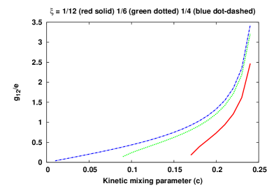
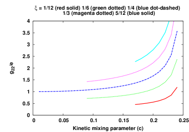
Figure 1: The couplings $g_{12}$ (left panel) and $g_{22}$ (right panel) of the dark photon $X_{2}^{\mu}$ as a function of the strength of kinetic mixing $c$ when $g_{11}=e$ and $g_{21}=0$. In both panels curves for several choices of $\xi$ (indicated in the legend) are shown. The allowed ranges are $|c|\leq\frac{1}{4}$ and $0\leq\xi\leq\frac{1}{2}$. However, as $\xi$ increases a more limited range of $c$ remains consistent.

As is evident from the above discussion both $g_{12}$ and $g_{22}$ are determined once $c$ and $\xi$ are fixed. Choosing several values of $\xi$ within the permitted range, we display in Fig. 1 the dependence of $g_{22}$ and $g_{12}$ on $c$. We have taken the central value of $\xi=1/4$ and also other values equidistantly at higher and lower sides of this central value. We have presented the results for five values of $\xi=$ 1/12 (red solid), 1/6 (green dotted), 1/4 (blue dot-dashed), 1/3 (magenta dotted), and 5/12 (blue solid). It is seen that for large $c\sim 1/4$ the two couplings are of comparable size. At the small $c$ end $g_{12}$ tends to zero while $g_{22}$ tends to a non-zero limiting value.

Both couplings diverge as $c$ tends towards $1/4$. This is a reflection of the factor $\sqrt{\lambda_{1}\lambda_{2}}$ in the denominator in the expressions for $g_{12}$ and $g_{22}$ in Eq. (48) since from Eq. (9):

$$\lambda_{1}\lambda_{2}=\frac{1}{16}-c^{2}\;\;.$$ (49)

Nonethesless physical processes remain finite in the $c\rightarrow 1/4$ limit as the mass of $X_{2}^{\mu}$ also diverges. Using Eqs. (29) and (45) one has:

$$m_{2}^{2}=e^{2}\xi^{2}(Q_{1}^{s2}+Q_{2}^{s2})\frac{1}{\lambda_{1}\lambda_{2}}v^{2}.$$ (50)

For any $\delta$ between 0 and $1/4$ when $\xi$ changes from $1/4-\delta$ to $1/4+\delta$ $\alpha_{1}$ and $\alpha_{2}$ are exchanged, as can be seen from Eq. (46). Because $g_{12}$ depends on the product $\alpha_{1}\alpha_{2}$, the curves for $g_{12}$ for these cases overlap. For a given value of $c$, larger $g_{22}$ corresponds to a higher $\xi$. Since $\alpha_{1,2}\leq 1$, we see from Eq. (46) that for larger values of $\xi$ the kinetic mixing strength $c$ can take values in a restricted range. Here we have considered only positive values of $c$ since, as noted, for negative $c$ one has $\alpha_{1}$ interchanged with $\alpha_{2}$ whereas $\lambda_{1}$ and $\lambda_{2}$ are exchanged. This will take $g_{12}$ to -$g_{12}$, while $g_{22}$ will be unaffected.

We observe that once $\alpha_{1}$ is fixed by $c$ and $\xi$, the electric charge of a fermion, $Q$, is given by Eq. (25) in terms of the $U(1)\times U(1)$ charges $Q_{1,2}$. The orthogonal charge combination, $Q^{\prime}$, is similarly defined in Eq. (28).

In the next two subsections we present two illustrative models. In the first one $U(1)_{sm}\times U(1)_{dm}$ breaks to $U(1)_{EM}$. Here suffixes $sm$ and $dm$ indicate visible and dark sectors respectively whereas the suffix $EM$ denotes electromagnetism. In the second example $U(1)_{EM}\times U(1)_{dm}$ breaks to $U(1)_{EM}$. In the first example gauge bosons of $U(1)_{sm}$ and $U(1)_{dm}$ mix during the spontaneous symmetry breaking process, whereas in the second case the mixing between photon and the dark gauge boson is solely due to the kinetic mixing.

V.2 Example 1: A toy model for dark matter

In this model there are two sectors, a visible sector denoted by $U(1)_{sm}$ and a dark sector denoted by $U(1)_{dm}$. Even though this model is not realistic as it stands, key features of our analysis can be demonstrated by this simplified version. Symmetry breaking is along the following line,

$$U(1)_{sm}\times U(1)_{dm}\longrightarrow U(1)_{EM}$$ (51)

To apply this formulation of kinetic mixing to models of dark matter we consider two classes of particles specified in terms of the nature of their charges $Q$ and $Q^{\prime}$. Of these, $Q$ corresponds to the current $\hat{J}^{\mu}_{1}$ which is associated with $U(1)_{EM}$. It is a conserved charge unlike $Q^{\prime}$ which corresponds to the orthogonal broken direction. The photon (${X}^{\mu}_{1}$) couples through only $Q$ while the dark photon (${X}^{\mu}_{2}$) couples to both $Q$ – coupling $g_{12}$ – as well as $Q^{\prime}$ – coupling $g_{22}$.

There are two classes of particles, namely, (a) Dark Matter which is decoupled from the photon by having $Q^{dm}=0$, and (b) Normal matter which has $Q^{\prime sm}=0$. By choice, we have the photon coupling only to the SM sector. It will be of our interest to discuss the coupling of SM with Dark Matter through the dark photon, $X_{2}^{\mu}$, mediated interactions. This is shown in the left panel of Fig. 2. For momentum transfers small compared to $m_{X^{2}}$ from Eqs. (48) the probability amplitude will be

$${\cal M}_{sm-dm}\propto\frac{g_{12}~{}Q^{sm}g_{22}~{}Q^{\prime dm}}{m_{X^{2}}^{2}}=-\left[e^{2}~{}Q^{sm}Q^{\prime dm}~{}\alpha_{1}\alpha_{2}\left(\sqrt{\frac{\lambda_{2}}{\lambda_{1}}}-\sqrt{\frac{\lambda_{1}}{\lambda_{2}}}\right)\frac{\xi}{\sqrt{\lambda_{1}\lambda_{2}}}\right]\frac{1}{m_{X^{2}}^{2}}\;\;,$$ (52)

where $Q^{sm}$ and $Q^{\prime dm}$ are respectively the electric charge of the SM particle and the dark charge of the DM particle.

One can readily extract the dependence of the above amplitude on $c$. One finds

$${\cal M}_{sm-dm}\propto\sqrt{16c^{2}-(4\xi-1)^{2}}\;.$$ (53)

By a suitable choice of $\xi$ near the limiting values

$$\xi\rightarrow 1/4\pm c,$$ (54)

the right-hand-side of Eq. (53) can be made arbitrarily small. Hence, a small and controllable interaction cross section between the standard and dark sectors is a natural consequence of the model. On the other hand, one may be tempted to think that for large values of the mixing parameter $|c|\sim 1/4$ this interaction can be enhanced. However, this will also modify cross sections of purely standard processes such as $e^{-}~{}e^{-}\rightarrow e^{-}~{}e^{-}$ and is very tightly constrained. For example, the $X_{2}^{\mu}$ coupling to SM fermions will result in interactions within the SM sector as depicted in the right panel of Fig. 2. This leads to the probability amplitude

$${\cal M}_{sm-sm}\propto\frac{(g_{12}~{}Q^{sm})^{2}}{m_{X^{2}}^{2}}=\left[e~{}Q^{sm}~{}\alpha_{1}\alpha_{2}\left(\sqrt{\frac{\lambda_{2}}{\lambda_{1}}}-\sqrt{\frac{\lambda_{1}}{\lambda_{2}}}\right)\right]^{2}\frac{1}{m_{X^{2}}^{2}}\;.$$ (55)

The dependence of the above amplitude on $c$ is

$${\cal M}_{sm-sm}\propto\left(16c^{2}-(4\xi-1)^{2}\right)\;.$$ (56)

Needless to say, one can similarly calculate scattering within the dark matter sector via $X_{2}^{\mu}$-exchange.

Figure 2: The interactions due to $X_{2}^{\mu}$ exchange: between SM particles and dark matter (left) and between SM particles themselves (right).

V.3 Example 2: Realistic $U(1)_{dm}$ mixing with QED

A simple and realistic model which appears in the literature of kinetic mixing is one in which the photon mixes with a $U(1)_{dm}$ gauge field. Because the other gauge boson is not yet detected experimentally, $U(1)_{dm}$ symmetry is broken and the dark photon is massive. Usually the mixing term is considered as a perturbation and its effects examined.

In our approach, which is exact, one must identify the remaining unbroken symmetry as QED which is also one of the two initial $U(1)$ symmetries. Thus, one must demand $X_{1}^{\mu}\equiv A_{1}^{\mu}$. From Eqs. (18), and (25) we can write

$$Q=q^{1}~{}(\alpha_{1}-\alpha_{2})\cos\phi+q^{2}~{}(\alpha_{1}+\alpha_{2})~{}\sin\phi\;.$$ (57)

The requirement that $Q=q^{1}$ can be achieved by

$${\rm Either}\;\;\left(\alpha_{1}=-\alpha_{2}={1\over\sqrt{2}}\;\;{\rm and}\;\;\phi\;={\pi\over 4}\right)\;\;{\rm or}\;\;(\phi=0\;\;{\rm and}\;\;\alpha_{2}=0)\;\;.$$ (58)

Of these, the second option is untenable as it implies $g_{2}=0$ as a consequence of Eq. (15).

This result identifies electric charge as the coupling of one of the factor groups that existed before symmetry breaking. From Eq. (15) it implies

$$g_{1}=g_{2}\equiv g,~{}~{}~{}~{}\tilde{g}_{1}=\frac{g}{2\sqrt{\lambda_{1}}},~{}~{}\tilde{g}_{2}=\frac{g}{2\sqrt{\lambda_{2}}}\;.$$ (59)

Thus, in the $A$ basis where gauge bosons have diagonal couplings with fermions, gauge coupling must be identical for the two $U(1)$ factors. To the best of our knowledge this is a new result. Then from Eqs. (34), (38) and (39),

$$g_{11} = g\equiv e\;\;,$$ (60)

$$g_{22} = e~{}\frac{1}{\sqrt{1-16c^{2}}}\;\;,$$ (61)

$$g_{12} = -e~{}\frac{4~{}c}{\sqrt{1-16c^{2}}}\;\;.$$ (62)

Using Eq. (44) we get $\xi=1/4$ for which as shown earlier $|c|\geq 0$.

Two noteworthy features here are that $g_{22}$, the coupling within the Dark Matter sector mediated by $X^{2}_{\mu}$, is stronger than normal electromagnetism. Also Dark Matter couples to ordinary matter via the coupling $g_{12}$ which goes to zero as the kinetic mixing parameter $c\rightarrow 0$.

Before moving on we would like to draw attention to another mode of handling kinetic mixing that is often used. It is common in the literature to define the mixing in the basis in which the gauge bosons are already the mass eigenstates, one of which is massless while the other has a non-zero mass typically through a Stückelberg mechanism. In such scenarios the removal of the kinetic mixing is enabled through the transformation

$$\pmatrix{A^{1}_{\mu}\cr~{}A^{2}_{\mu}}=\pmatrix{1&{-4c\over\sqrt{1-16c^{2}}}\cr 0&{1\over\sqrt{1-16c^{2}}}}\pmatrix{{X}^{1}_{\mu}\cr{X}^{2}_{\mu}}.$$ (63)

Note that this leads precisely to the couplings in eqs. (62) for ${X}^{1}_{\mu}$ and ${X}^{2}_{\mu}$.

VI Summary and conclusion

When a theory has two (or more) $U(1)$ symmetries then the possibility of gauge kinetic mixing opens up. We have examined kinetic mixing in a generic model with two $U(1)$ factors where the symmetry is spontaneously broken as $U^{1}(1)\times U^{2}(1)\rightarrow U^{3}(1)$. These models are usually considered in the literature using various approaches that commonly assume a small mixing parameter, $c$, and study physical effects by varying it. In this paper in contrast we have focussed on $c$ without restricting it to be small. We show that in certain cases the range of $c$ is bounded.

Here, as a first step the kinetic mixing term is removed by an orthogonal rotation and a scaling. It is convenient to use the charges, $Q_{1,2}$, of fermions and scalars in this new orthonormal basis to discuss the spontaneous symmetry breaking. The symmetry breaking identifies a charge, $Q=\alpha_{1}Q_{1}+\alpha_{2}Q_{2}$, corresponding to the unbroken gauge symmetry. The interactions are then readily expressed in terms of $Q$ and an orthogonal charge $Q^{\prime}$. While the massless gauge boson couples only to $Q$ (with coupling $g_{11}$) the heavy gauge boson has a coupling to $Q^{\prime}$ of strength $g_{22}$ and also to $Q$ given by $g_{12}$. We derive analytical formulae for these couplings and show that both $g_{12}$ and $g_{22}$ are controlled by the mixing parameter $c$. An important result, which can be seen from Fig. 1 is the following. To be able to identify the unbroken $U(1)$ coupling with that of electromagnetism for a fixed $\xi=(g_{1}^{2}+g_{2}^{2})/8e^{2}$ there is a lower bound on the magnitude of $c$ given in Eq. (47). The bound is quoted in a basis where couplings of fermions to gauge bosons is diagonal.

As noted, a nonzero $g_{12}$ is responsible for interactions between the dark and ordinary sectors. The coupling $g_{22}$ leads to interactions within the dark sector which have been suggested as an ingredient for the explanation of the halo structure of satellite galaxies [16]. We note that $g_{22}$ need not be a small coupling unlike $g_{12}$, which is controlled by kinetic mixing. Such self-interaction is also needed to resolve conflicts between observation and simulation at the galactic scale and smaller [14]. Self-interaction in the dark sector is also needed to explain signals obtained in the DAMA experiment [15].

We have illustrated this theory by two examples related to Dark Matter. In both cases we have identified the unbroken $U(1)$ as the electromagnetic group $U(1)_{EM}$. In the first example, ordinary matter has only the $Q$ charge, which is now the electric charge, whereas dark matter has only the $Q^{\prime}$ charge. The heavy gauge boson is identified with the dark photon and it couples to visible as well as dark matter. We have shown the manner in which the coupling of the dark photon to the ordinary matter depends on the mixing parameter $c$. In the limit of no kinetic mixing the dark photon does not interact with the ordinary matter at all (except by gravity) and therefore cannot be searched easily in scattering experiments. In the second example we have examined the case where $U(1)_{EM}$ is kinetically mixed with another $U(1)$. This situation can occur only when the two gauge groups have same gauge couplings initially. In this model also we have given analytical formulae for the coupling strengths of heavy and massless gauge bosons. In both cases we have derived analytical expressions for the Dark Matter self-coupling strengths.

The dark photon has been considered here as an intermediary in interactions linking dark matter with ordinary matter. There is also the possibility that a dark photon may be produced on-shell in physical processes, e.g., in dark matter annihilation. In the literature it has been proposed to look for comparatively light dark photon signals using $e^{+}e^{-}$ colliders or electron beam dump experiments where an emitted dark photon could decay to a pair of lighter dark matter [17]. If the dark photon coupling to dark matter is enhanced to large values by an appropriate choice of the mixing parameter $c$, as indicated in sec. V.3, decays to dark matter will become more prominent. This will permit the dark photon to be detected through these proposed tests.

If the dark photon is relatively light, having mass around 10 MeV, then it can decay to $e^{+}e^{-}$ pairs only, i.e., with branching ratio unity, with a lifetime which goes as $1/c^{2}$. Detection of electron-positron pairs with invariant mass matching the dark photon mass would be a clear signal. If the mass is such that $\mu^{+}\mu^{-}$ decays are kinematically possible then that too could be an alternate detection channel. As formulated, the dark photon coupling to all SM particles should be proportional to the respective electric charges. So, the branching ratio to muons and electrons will differ simply due to the phase space considerations. Electrons and muons of such energy can be observed in neutrino detectors, e.g., SuperKamiokande. If the dark photons are produced in the annihilation of much heavier dark matter particles then one can expect them to be relativistic. In such an event, the decay products will be collimated in the forward direction. A magnetic field will help in separating the decay products and also determine their energy-momentum. A sufficiently high-energy charged particle, e.g., at an accelerator, will emit dark photons by bremsstahlung which, needless to say, will be suppressed compared to similar $\gamma$ emission by a factor of (${\cal O}(c^{2})$). There are therefore several avenues for testing the scenario of kinetic mixing discussed in this paper.

Acknowledgments: The authors are grateful to Professor E. Ma for stoking their curiosity on the role of kinetic mixing in the dark photon models. BB would like to thank E.J. Chun for discussions. The research of AR is supported by a J.C. Bose Fellowship of the Department of Science and Technology of the Government of India.

References

- [1] B. Holdom, Phys. Lett. B166, 196 (1986).
- [2] F. del Aguila, G. D. Coughlan and M. Quiros, Nucl. Phys. B 307, 633 (1988) [Erratum-ibid. B 312, 751 (1989)]; T. G. Rizzo, Phys. Rev. D 59, 015020 (1998) [hep-ph/9806397]; S. Bertolini, L. Di Luzio and M. Malinsky, Phys. Rev. D 80, 015013 (2009)[arXiv:0903.4049 [hep-ph]]; J. Chakrabortty and A. Raychaudhuri, Phys. Rev. D 81, 055004 (2010); R. M. Fonseca, M. Malinsky and F. Staub, Phys. Lett. B 726, 882 (2013).
- [3] K. S. Babu, C. F. Kolda and J. March-Russell, Phys. Rev. D 57, 6788 (1998); D. Feldman, Z. Liu, P. Nath, Phys. Rev. D75, 115001 (2007); E. J. Chun, J. -C. Park and S. Scopel, JHEP 1102, 100 (2011).
- [4] J. D. Bjorken, R. Essig, P. Schuster and N. Toro, Phys. Rev. D 80, 075018 (2009).
- [5] S. A. Abel, M. D. Goodsell, J. Jaeckel, V. V. Khoze and A. Ringwald, JHEP 0807, 124 (2008) [arXiv:0803.1449 [hep-ph]]; M. Pospelov and A. Ritz, Phys. Lett. B671, 391 (2009); M. Pospelov, Phys. Rev. D 80, 095002 (2009); C. Cheung, J. T. Ruderman, L. -T. Wang and I. Yavin, Phys. Rev. D 80, 035008 (2009) [arXiv:0902.3246 [hep-ph]]; Y. Mambrini, JCAP 1009, 022 (2010) [arXiv:1006.3318 [hep-ph]]; R. Foot, Phys. Lett. B 718, 745 (2013) [arXiv:1208.6022 [astro-ph.CO]]; H. An, M. Pospelov and J. Pradler, Phys. Lett. B 725, 190 (2013); C. -F. Chang, E. Ma and T. -C. Yuan, S.N. Gninenko, arXiv1301.7555v3 [hep-ph]; J. Redondo and G. Raffelt, JCAP 1308, 034 (2013).
- [6] P. Crivelli, A. Belov, U. Gendotti, S. Gninenko and A. Rubbia, JINST 5, P08001 (2010); P. Adlarson et al. [WASA-at-COSY Collaboration], Phys. Lett. B 726, 187 (2013); P. H. Adrian, arXiv:1301.1103 [physics.ins-det]; S. Andreas, S. V. Donskov, P. Crivelli, A. Gardikiotis, S. N. Gninenko, N. A. Golubev, F. F. Guber and A. P. Ivashkin et al., arXiv:1312.3309 [hep-ex].
- [7] S. Y. Choi, C. Englert and P. M. Zerwas, Eur. Phys. J. C 73, 2643 (2013) [arXiv:1308.5784 [hep-ph]].
- [8] S. Cassel, D. M. Ghilencea and G. G. Ross, Nucl. Phys. B 827, 256 (2010) [arXiv:0903.1118 [hep-ph]].
- [9] See, for example, B. Patt and F. Wilczek, hep-ph/0605188; B. Batell, M. Pospelov and A. Ritz, Phys. Rev. D 80, 095024 (2009) [arXiv:0906.5614 [hep-ph]]; C. Englert, T. Plehn, D. Zerwas and P. M. Zerwas, Phys. Lett. B 703, 298 (2011) [arXiv:1106.3097 [hep-ph]].
- [10] See, for example, the review article, V. Trimble, Ann. Rev. Astron. Astrophys. 25, 425 (1987), and references therein.
- [11] C.L. Bennett, A. Banday, K.M. Gorski, G. Hinshaw, P. Jackson, P. Keegstra, A. Kogut, George F. Smoot, D.T. Wilkinson, E.L. Wright Astrophys.J. 464 L1-L4 (1996); WMAP Collaboration (E. Komatsu (Texas U.) et al.), Astrophys. J. Suppl. 192, 18 (2011).
- [12] Planck Collaboration (P.A.R. Ade (Cardiff U.) et al.). e-Print: arXiv:1303.5076 [astro-ph.CO].
- [13] M. Pospelov, A. Ritz, M. B. Voloshin, Phys. Lett. B662, 53 (2008).
- [14] D. N. Spergel and P. J. Steinhardt, Phys. Rev. Lett. 84, 3760 (2000); R. Dave, D. N. Spergel, P. J. Steinhardt and B. D. Wandelt, Astrophys. J. 547, 574 (2001) [astro-ph/0006218]; M. R. Buckley and P. J. Fox, Phys. Rev. D81, 083522 (2010); S. L. Shapiro and V. Paschalidis, Phys. Rev. D 89, 023506 (2014) [arXiv:1402.0005 [astro-ph.CO]].
- [15] S. Mitra, Phys. Rev. D 71, 121302 (2005); A. K. Ganguly, P. Jain, S. Mandal, S. Stokes, Phys. Rev. D76, 025026 (2007); R. Bernabei, P. Belli, A. Di Marco, F. Montecchia, F. Cappella, A. d’Angelo, A. Incicchitti, D. Prosperi, R. Cerulli, C.J. Dai, Nucl. Instrum. Meth. A692, 120 (2012).
- [16] See, for example, A. Loeb and N. Weiner, Phys. Rev. Lett. 106, 171302 (2011).
- [17] R. Essig, J. Mardon, M. Papucci, T. Volansky and Y. -M. Zhong, JHEP 1311, 167 (2013) [arXiv:1309.5084 [hep-ph]]; B. Batell, R. Essig and Z. ’e. Surujon, arXiv:1406.2698 [hep-ph]; E. Izaguirre, G. Krnjaic, P. Schuster and N. Toro, Phys. Rev. D 88, 114015 (2013) [arXiv:1307.6554 [hep-ph]]; arXiv:1403.6826 [hep-ph].