Nonequilibrium stationary states of 3D self-gravitating systems

Abstract

Three dimensional self-gravitating systems do not evolve to thermodynamic equilibrium, but become trapped in nonequilibrium quasistationary states. In this Letter we present a theory which allows us to a priori predict the particle distribution in a final quasistationary state to which a self-gravitating system will evolve from an initial condition which is isotropic in particle velocities and satisfies a virial constraint $2K=-U$, where $K$ is the total kinetic energy and $U$ is the potential energy of the system.

Unlike systems with short-range forces which relax to thermodynamic equilibrium starting from an arbitrary initial condition, systems with long-range interactions become trapped in nonequilibrium quasistationary states (QSS) the lifetime of which diverges with the number of particles Chandrasekhar (1941); Konishi and Kaneko (1992); Latora et al. (1998, 2000); Yamaguchi et al. (2004); Jain et al. (2007); Antoniazzi et al. (2007); Gabrielli et al. (2010); Chavanis (2013). For interaction potentials unbounded from above, the QSS have been observed to have a characteristic core-halo structure Levin et al. (2014). The extent of the halo is determined by the parametric resonances which arise from the collective density oscillations during the relaxation process Gluckstern (1994). The dynamics of 3D self-gravitating systems, however, is significantly more complex due to the existence of unbound states Padmanabhan (1990); Levin et al. (2008). Indeed, Newton’s gravitational potential is bounded from above, so that the parametric resonances may actually transfer enough energy to allow some particles to completely escape from the gravitational cluster Levin et al. (2008); Joyce et al. (2009). This makes the study of 3D self-gravitating systems particularly challenging Chavanis and Bouchet (2005); Champion et al. (2014). Recently, however, it was shown that if the initial particle distribution function is isotropic in velocity and satisfies the, so called, virial condition (VC), density oscillations and parametric resonances will be suppressed Teles et al. (2010, 2011); Joyce and Worrakitpoonpon (2011); Benetti et al. (2012). The relaxation to equilibrium will then proceed adiabatically. In the thermodynamic limit, each particle of the gravitational cluster will evolve under the action of a quasistatic mean-field potential and the phase-mixing of particle trajectories will lead to a nonequilibrium QSS. In this Letter we will show that it is possible to a priori predict the density and the velocity distribution functions within the QSS to which a 3D gravitational system will evolve if the initial distribution is isotropic in particle velocities and satisfies VC.

The virial theorem requires that a stationary gravitational system must have $2K=-U$, where $K$ is the total kinetic energy and $U$ is the potential energy. This, however does not mean that an arbitrary initial distribution which satisfies the VC will remain stationary. To be stationary, a distribution function must be a time-independent solution of the collisionless Boltzmann (Vlasov) equation Braun and Hepp (1977); Campa et al. (2009); Rocha Filho et al. (2014). From Jeans’ theorem, this will only be the case if the distribution depends on the phase space coordinates solely through the integrals of motion Binney and Tremaine (2008). Recently, however, it was shown that if the initial particle distribution $f_{0}(\mathbf{r},\mathbf{p})$ is spherically symmetric and isotropic in velocity, $f_{0}(\mathbf{r},\mathbf{p})=f_{0}(r,p)$, and satisfies the VC, strong density oscillations will be suppressed and the relaxation to QSS will be intrinsically different than for initial distributions which do not satisfy VC Yamaguchi (2008); Levin et al. (2014). In principle, a spherically symmetric distribution does not need to be a function of the modulus of momentum. A spherical symmetry is compatible with the distribution being a function of both radial and angular momentum independently. The assumption of isotropicity is included to prevent the radial orbit instability (ROI) which leads to spontaneous symmetry breaking of the distribution function. ROI can occur when kinetic energy of the system is dominated by the radial velocity component Aguilar and Merritt (1990); Barnes et al. (2009). On the other hand, for isotropic velocity distributions symmetry breaking occur only when the initial distribution deviates strongly from VC Pakter et al. (2013). For initial particle distributions isotropic in velocity and satisfying the VC, relaxation to equilibrium is a consequence of phase mixing of particle trajectories Ribeiro-Teixeira et al. (2014), while for non-virial initial conditions relaxation results from excitation of parametric resonances Gluckstern (1994) and a nonlinear Landau damping Villani (2014); Levin et al. (2014).

Consider a spherically symmetric — in both positions and velocities — initial phase space particle distribution. We will work in the thermodynamic limit $N\rightarrow\infty$, $m\rightarrow 0$, while $mN=M$, where $N$ is the total number of particles, $m$ is the mass of each particle, and $M$ is the total mass of the gravitational system. At $t=0$ the particles are distributed in accordance with the initial distribution $f_{0}(r,p)$ inside an infinite 3D configuration space. We would like to predict the distribution function for the system when it relaxes to a QSS. It is easy to see that in the thermodynamic limit the positional correlations between the particles vanish and all the dynamics is controlled by the mean-field potential Rocha Filho et al. (2014). Furthermore, if the initial distribution is such that the VC is satisfied, the mean-field potential should vary adiabatically and the energy of each particle should change little. Since the mean-field potential is a nonlinear function of position, the particles on the energy shell $[\mathcal{E},\mathcal{E}+d\mathcal{E}]$ with slightly distinct one-particle energies $\mathcal{E}$ will have incommensurate orbital frequencies. This means that after a transient period, the phase-mixing will result in a uniform particle distribution over the energy shell. The particle distribution in the final QSS can then be obtained by a coarse-graining of the initial distribution over the phase space available to the particle dynamics, taking into account the conservation of the angular momentum of each particle, given the spherical symmetry of the mean-field potential.

Consider an arbitrary initial particle distribution $f_{0}(r,p)$ that satisfies VC. For $t>0$ the particles will evolve under the action of an external adiabatically varying potential $\varphi(r,t)$ which will eventually converge to some $\psi(r)$. Our approach will be to construct a coarse-grained distribution for particles evolving directly under the action of the static potential $\psi(r)$ which will then be calculated self-consistently Leoncini et al. (2009); de Buyl et al. (2011a, b). Clearly such an approximation will only work if the variation of $\varphi(r,t)$ is adiabatic and no resonances are excited. This is precisely the case for the initial distributions which are isotropic in velocity and satisfy VC Ribeiro-Teixeira et al. (2014).

Since $\psi(r)$ is static and spherically symmetric, the energy and the angular momentum of each particle will be preserved. The nonlinearity of $\psi(r)$ will lead to phase-mixing of particle trajectories with the same energy and angular momentum. The number of particles with energy between $[\mathcal{E},\mathcal{E}+d\mathcal{E}]$ and the square of the angular momentum between $[\ell^{2},\ell^{2}+d\ell^{2}]$ is $n(\mathcal{E},\ell^{2})d\mathcal{E}d\ell^{2}$ and is conserved throughout dynamics. In the QSS these particles will spread over the phase space volume $g(\mathcal{E},\ell^{2})d\mathcal{E}d\ell^{2}$, so that the coarse-grained distribution function for the QSS will be

$$f(\mathcal{E},\ell^{2})=\frac{n\!\left(\mathcal{E},\ell^{2}\right)}{g\!\left(\mathcal{E},\ell^{2}\right)}$$ (1)

The self-consistent potential $\psi(r)$ must satisfy the Poisson equation,

$$\frac{1}{r^{2}}\frac{\mathrm{d}}{\mathrm{d}r}\left(r^{2}\frac{\mathrm{d}\psi}{\mathrm{d}r}\right)=4\pi Gm\rho(r)$$ (2)

where

$$\rho({\bf r})=\int d^{3}p\,\,\,f\left[\mathcal{E}({\bf r},{\bf p}),\ell^{2}({\bf r},{\bf p})\right]$$ (3)

is the asymptotic particle density. This gives us a closed set of equations which can be used to calculate the distribution function in the QSS. To simplify the notation we will scale all the distances to an arbitrary length scale $L_{0}$, time to $\sqrt{L_{0}^{3}/GM}$, the potential to $GM/L_{0}$, and the energy to $GM^{2}/L_{0}$.

Because of the conservation of the angular momentum of each particle, it is convenient to work with the canonical positions $(r,\theta,\phi)$ and conjugate momenta $(p_{r},p_{\theta},p_{\phi})$. Note that in terms of these variables the invariant phase space measure is $\mathrm{d}^{3}x\mathrm{d}^{3}p=\,\mathrm{d}r\,\mathrm{d}\theta\,\mathrm{d}\phi\,\,\mathrm{d}p_{r}\,\mathrm{d}p_{\theta}\,\mathrm{d}p_{\phi}$. The particle energy and square modulus of the angular momentum are

$$\epsilon(r,\theta,p_{r},p_{\theta},p_{\phi}) =\frac{1}{2}\left(p_{r}^{2}+\frac{p_{\theta}^{2}}{r^{2}}+\frac{p_{\phi}^{2}}{r^{2}\sin^{2}\theta}\right)+\psi(r),$$ (4)

$$l^{2}(\theta,p_{\theta},p_{\phi}) =p_{\theta}^{2}+\frac{p_{\phi}^{2}}{\sin^{2}\theta}$$ (5)

respectively. The density of states $g(\mathcal{E},\ell^{2})$ is

$$g(\mathcal{E},\ell^{2}) =\int\!\!\,\mathrm{d}p_{r}\,\mathrm{d}p_{\theta}\,\mathrm{d}p_{\phi}\!\int\!\!\,\mathrm{d}r\,\mathrm{d}\theta\,\mathrm{d}\phi\,\,\delta\left[\ell^{2}\!-l^{2}(\theta,p_{\theta},p_{\phi})\right]$$

$$\quad\times\delta\left[\mathcal{E}-\epsilon(r,\theta,p_{r},p_{\theta},p_{\phi})\right]$$ (6)

and the particle phase space density $n(\mathcal{E},\ell^{2})$ is

$$n(\mathcal{E} ,\ell^{2})=\int\,\mathrm{d}p_{r}\,\mathrm{d}p_{\theta}\,\mathrm{d}p_{\phi}\int\,\mathrm{d}r\,\mathrm{d}\theta\,\mathrm{d}\phi\,\delta\!\left[\ell^{2}-l^{2}(\theta,p_{\theta},p_{\phi})\right]$$

$$\times\delta\!\left[\mathcal{E}-\epsilon(r,\theta,p_{r},p_{\theta},p_{\phi})\right]$$

$$\times f_{0}\!\left(r,\sqrt{p_{r}^{2}+\frac{p_{\theta}^{2}}{r^{2}}+\frac{p_{\phi}^{2}}{r^{2}\sin^{2}\theta}}\right).$$ (7)

Integration over all the variables in Eqs. (Nonequilibrium stationary states of 3D self-gravitating systems) and (Nonequilibrium stationary states of 3D self-gravitating systems), other than $\,\mathrm{d}r$, can be performed with the help of a Dirac delta function identity

$$\delta[f(x)]=\frac{\sum_{i}\delta(x-x_{i})}{|f^{\prime}(x_{i})|},$$ (8)

where $x_{i}$ is the $i$’th root of $f(x)$. Carrying out the integration we obtain the coarse-grained distribution function for the QSS,

$$f(\mathcal{E},\ell^{2})=\frac{\int\,\mathrm{d}r\,f_{0}\!\left[r,\sqrt{2\big{(}\mathcal{E}-\psi(r)}\big{)}\right]\frac{\Theta\left[\mathcal{E}-\frac{\ell^{2}}{2r^{2}}-\psi(r)\right]}{\sqrt{\mathcal{E}-\frac{\ell^{2}}{2r^{2}}-\psi(r)}}}{\int\,\mathrm{d}r\,\frac{\Theta\left[\mathcal{E}-\frac{\ell^{2}}{2r^{2}}-\psi(r)\right]}{\sqrt{\mathcal{E}-\frac{\ell^{2}}{2r^{2}}-\psi(r)}}},$$ (9)

where $\Theta$ is the Heaviside step function. The coarse-grained distribution function depends on position and momentum only through the conserved quantities $\mathcal{E}$ and $\ell^{2}$; therefore, it is automatically a stationary solution of the Vlasov equation.

The Poisson equation can be rewritten as

$$r^{2}\frac{\mathrm{d}^{2}\psi}{\mathrm{d}r^{2}}+2r\frac{\mathrm{d}\psi}{\mathrm{d}r}=N(r)$$ (10)

where $N(r)=4\pi r^{2}\rho(r)$, or

$$N(r)=\int\!\!\,\mathrm{d}p_{r}\,\mathrm{d}p_{\theta}\,\mathrm{d}p_{\phi}\!\int\!\!\,\mathrm{d}\theta\,\mathrm{d}\phi\,f\!\left(\mathcal{E},\ell^{2}\right).$$ (11)

Multiplying Eq (11) by the identity

$$\int\,\mathrm{d}(\ell^{2})\,\delta\!\left(\ell^{2}-p_{\theta}^{2}-\frac{p_{\phi}^{2}}{\sin^{2}\theta}\right)=1\,,$$ (12)

and changing the order of integration, we can write

$$N(r) =\int\!\!\,\mathrm{d}(\ell^{2})\,\mathrm{d}p_{r}\,\mathrm{d}p_{\theta}\,\mathrm{d}p_{\phi}\!\int\!\!\,\mathrm{d}\theta\,\mathrm{d}\phi\,\,\delta\!\left(\ell^{2}-p_{\theta}^{2}-\frac{p_{\phi}^{2}}{\sin^{2}\theta}\right)$$

$$\times f\!\left(\frac{p_{r}^{2}}{2}+\frac{p_{\theta}^{2}}{2r^{2}}+\frac{p_{\phi}^{2}}{2r^{2}\sin^{2}\theta}+\psi(r),p_{\theta}^{2}+\frac{p_{\phi}^{2}}{\sin^{2}\theta}\right)\,.$$ (13)

The integration over the variables $p_{\theta}$, $p_{\phi}$, $\theta$, $\phi$ can now be performed explicitly with the help of Eq. (8). Finally, changing the integration variable from $p_{r}$ to $\mathcal{E}$, Eq. (Nonequilibrium stationary states of 3D self-gravitating systems) simplifies to

$$N(r)=8\pi^{2}\int\limits_{0}^{\infty}\,\mathrm{d}(\ell^{2})\int\limits_{\mathcal{E}_{0}}^{\infty}\,\mathrm{d}\mathcal{E}\,f\left(\mathcal{E},\ell^{2}\right)\frac{\Theta\left[\mathcal{E}-\frac{\ell^{2}}{2r^{2}}-\psi(r)\right]}{\sqrt{2\left(\mathcal{E}-\frac{\ell^{2}}{2r^{2}}-\psi(r)\right)}}$$ (14)

where the lower limit of integration is $\mathcal{E}_{0}=\frac{\ell^{2}}{2r^{2}}+\psi(r)$ and $f\left(\mathcal{E},\ell^{2}\right)$ is given by Eq (9). Substituting Eq. (14) into Eq. (10), we find an integro-differential equation for the gravitational potential $\psi(r)$ in the QSS. Eq. (10) can be solved numerically using Picard iteration. Once the gravitational potential is known, the coarse-grained distribution function can be easily calculated by performing the integration in Eq. (9).

We next validated the proposed theory by comparing the marginal position and velocity distribution functions $N(r)$ and $N(p)$ to explicit molecular dynamics (MD) simulations of a 3D self-gravitating system of $N$ particles. The simulations were performed using a version of particle-in-cell (PIC) algorithm, in which each particle interacts with a mean-field potential produced by all other particles Levin et al. (2014). In the absence of ROI this simulations produce identical particle distributions in QSS as calculated using traditional binary interaction methods, but are three orders of magnitude faster. This allows us to easily reach the QSS Sup . The density distribution $N(r)$ is given by Eq (14). To obtain the momentum distribution we first calculate the distribution

$$N(p_{r})=\int\!\!\,\mathrm{d}r\,\mathrm{d}p_{\theta}\,\mathrm{d}p_{\phi}\!\int\!\!\,\mathrm{d}\theta\,\mathrm{d}\phi\,f\!\left(\mathcal{E},\ell^{2}\right)\,,$$ (15)

where $\mathcal{E}=p_{r}^{2}/2+\frac{\ell^{2}}{2r^{2}}+\psi(r)$ and $\ell^{2}=p_{\theta}^{2}+\frac{p_{\phi}^{2}}{\sin^{2}\theta}$. The change of variable from $p_{r}$ to the modulus of momentum $p$ can be performed with the help of Eq. (12) and the identity

$$\int\,\mathrm{d}p^{2}\,\delta\!\left(p^{2}-p_{r}^{2}-\frac{\ell^{2}}{r^{2}}\right)=1$$ (16)

yielding,

$$N(p)=8\pi^{2}p\int\limits_{0}^{\infty}\,\mathrm{d}(\ell^{2})\int\limits_{0}^{\infty}\,\mathrm{d}r\,f\left(\mathcal{E},\ell^{2}\right)\frac{\Theta\left[p^{2}-\frac{\ell^{2}}{r^{2}}\right]}{\sqrt{p^{2}-\frac{\ell^{2}}{r^{2}}}}\,$$ (17)

where $\mathcal{E}=p^{2}/2+\psi(r)$.

We first consider a waterbag initial distribution,

$$f_{0}(r,p)=\eta\,\Theta\left(r_{m}^{2}-r^{2}\right)\Theta\left(p_{m}^{2}-p^{2}\right).$$ (18)

where $\eta=9/(16\pi^{2}r_{m}^{3}p_{m}^{3})$ is the normalization constant. We will measure all the lengths in units of $r_{m}$, which is equivalent to setting $r_{m}=1$. The VC requires that $2K=-U$, where

$$K=\frac{1}{2}\int\mathrm{d}^{3}r\,\mathrm{d}^{3}p\,f_{0}(r,p)\,p^{2}$$ (19)

is the kinetic energy and

$$U=\frac{1}{2}\int\mathrm{d}^{3}r\,\mathrm{d}^{3}p\,f_{0}(r,p)\,\psi_{0}(r)$$ (20)

is the potential energy of the system. The potential $\psi_{0}(r)$ for the initial waterbag distribution is

$$\psi_{0}(r)=\begin{cases}\frac{r^{2}-3}{2}&\text{if }r<1\\ -\frac{1}{r}&\text{if }r\geq 1.\end{cases}$$ (21)

Using Eqs (18) and (21) to calculate $K$ and $U$, the VC reduces to $p_{m}=1$. In Fig 1 we plot the joint distribution function $f(\mathcal{E},\ell^{2})$ for the QSS.

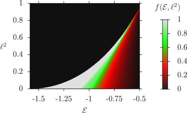
Figure 1: Distribution function in energy and angular momentum for the QSS, for an initial waterbag distribution, Eq (18), satisfying VC.

The marginal distribution functions can be calculated using Eqs (14) and (17) together with Eq (9). Fig 2 shows the position and velocity distributions $N(r)$ and $N(p)$ predicted by the integrable model. The symbols are the results of molecular dynamics (MD) simulations. An excellent agreement between the theory and the simulations can be seen.

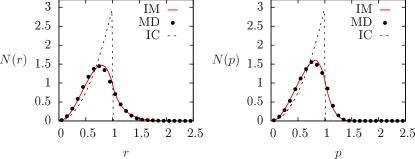
Figure 2: Theoretically predicted density (left) and momentum (right) distributions (solid lines) for the QSS for the initial waterbag distribution. The symbols (black dots) are the results of MD simulations. The initial $t=0$ density and momentum distributions are plotted with dashed lines – an initial waterbag distribution is given by Eq (18).

One particularly nice feature of the present theory is that it can be easily used to predict the final QSS for any initial distribution as long as it satisfies VC. We next study a parabolic initial distribution, given by

$$f_{0}\left(r,p\right)=\eta\left(1-r^{2}\right)\Theta\!\left(1-r^{2}\right)\Theta\!\left(p_{m}^{2}-p^{2}\right)$$ (22)

with $\eta=45/(32\pi^{2}p_{m}^{3})$. The VC for this distribution is $p_{m}=5/\sqrt{21}$. The marginal distributions predicted by the theory are compared with simulations in Fig 3. Once again the agreement is very good.

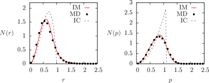
Figure 3: Solid lines are the theoretically predicted density (left) and momentum (right) distributions for the QSS for initial distribution (dashed lines) given by Eq. (22). The symbols (black dots) are the results of MD simulations.

For strongly inhomogeneous initial distributions, VC is not enough to completely prevent the temporal dynamics of the mean-field potential. That is, even if we restrict one moment of the distribution function, other moments might still have sufficiently strong dynamics to excite parametric resonances. Indeed, we find that for very strongly inhomogeneous initial distributions, there is some discrepancy between the theory and the simulations. Nevertheless even in these extreme cases the theory remains quite accurate Sup .

We have presented a theory that is able to predict the particle distribution in the final QSS to which a 3D self-gravitating system will relax from an initial condition. The theory can be used for initial distributions which are isotropic in particle velocity and satisfy the VC.

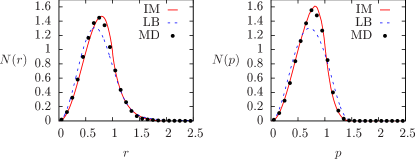
Figure 4: Comparison between the density (left) and momentum (right) distributions calculated using LB statistics and the present theory. Initial distribution is the waterbag in momentum and position, Eq (18), satisfying VC. Solid curves are the results of the present theory, dashed curves are the predictions of LB theory, and the solid circles are the results of MD simulations.

It is interesting to compare and contrast our approach with the theory of violent relaxation developed by Lynden-Bell (LB). The statistical mechanics of LB is based on the assumption of ergodicity and perfect mixing of the density levels of the initial distribution function over the phase space Lynden-Bell (1967). This is contrary to the approach presented in this Letter which shows that dynamics of 3D self-gravitating systems with initial distribution satisfying the virial condition is closer to integrable than ergodic.

Curiously for various systems, in which the particles are either self-bound — like 1d and 2d gravity — or are bounded by an external potential or by the topology — such as magnetically confined plasmas or spin systems — the LB approach was found to work best for the initial waterbag distributions that satisfied the VC Levin et al. (2014); Benetti et al. (2012). For distributions away from VC, QSS were found to have a characteristic core-halo structure very different from the predictions of LB theory Teles et al. (2010, 2011); Joyce and Worrakitpoonpon (2011); Pakter and Levin (2011); Figueiredo et al. (2014). It was recently observed, however, that for more complex inhomogeneous or multilevel distributions LB theory failed even when the initial distribution function satisfied VC Ribeiro-Teixeira et al. (2014); Pakter and Levin (2013). The failure of LB theory can now be attributed to the the almost complete absence of ergodicity and mixing when the initial distribution satisfies VC. The evolution of the mean-field potential of such systems is almost adiabatic and the dynamics is closer to integrable than to ergodic Ribeiro-Teixeira et al. (2014). The relaxation to QSS is the result of phase-mixing of particles on the same energy shells and not a consequence of ergodicity over the full energy surface. Indeed for 3D gravitational systems LB theory fails to accurately account for either velocity or density distributions, as can be seen in Fig. 4, even for the initial virial waterbag distribution, Eq. (18). Furthermore, LB theory is very difficult to extent to more complicated initial conditions than a one-level waterbag distribution, while the present approach can, in principle, be used for any arbitrary distribution as long as it satisfies VC. The goal of the future work will be to extend the theory presented in this Letter to initial distributions which do not satisfy VC. Parametric resonances and particle evaporation, however, make this a very difficult task.

This work was partially supported by the CNPq, FAPERGS, CAPES, INCT-FCx, and by the US-AFOSR under the grant FA9550-12-1-0438.

References

- Chandrasekhar (1941) S. Chandrasekhar, Astrophy. J. 93, 285 (1941).
- Konishi and Kaneko (1992) T. Konishi and K. Kaneko, Journal of Physics A: Mathematical and General 25, 6283 (1992).
- Latora et al. (1998) V. Latora, A. Rapisarda, and S. Ruffo, Phys. Rev. Lett. 80, 692 (1998).
- Latora et al. (2000) V. Latora, A. Rapisarda, and S. Ruffo, Physica A 280, 81 (2000).
- Yamaguchi et al. (2004) Y. Y. Yamaguchi, J. Barré, F. Bouchet, T. Dauxois, and S. Ruffo, Physica A 337, 36 (2004).
- Jain et al. (2007) K. Jain, F. Bouchet, and D. Mukamel, J. Stat. Mech. Theor. Exp. 2007, P11008 (2007).
- Antoniazzi et al. (2007) A. Antoniazzi, D. Fanelli, J. Barré, P.-H. Chavanis, T. Dauxois, and S. Ruffo, Phys. Rev. E 75, 011112 (2007).
- Gabrielli et al. (2010) A. Gabrielli, M. Joyce, and B. Marcos, Phys. Rev. Lett. 105, 210602 (2010).
- Chavanis (2013) P.-H. Chavanis, Astron. Astrophys. 556, A93 (2013).
- Levin et al. (2014) Y. Levin, R. Pakter, F. B. Rizzato, T. N. Teles, and F. P. C. Benetti, Phys. Rep. 535, 1 (2014).
- Gluckstern (1994) R. L. Gluckstern, Phys. Rev. Lett. 73, 1247 (1994).
- Padmanabhan (1990) T. Padmanabhan, Phys. Rep. 188, 285 (1990).
- Levin et al. (2008) Y. Levin, R. Pakter, and F. B. Rizzato, Phys. Rev. E 78, 021130 (2008).
- Joyce et al. (2009) M. Joyce, B. Marcos, and F. Sylos Labini, Mon. Not. R. Astron. Soc. 397, 775 (2009).
- Chavanis and Bouchet (2005) P. Chavanis and F. Bouchet, Astron. Astrophys. 430, 771 (2005).
- Champion et al. (2014) M. Champion, A. Alastuey, T. Dauxois, and S. Ruffo, J. Phys. A 47, 225001 (2014).
- Teles et al. (2010) T. N. Teles, Y. Levin, R. Pakter, and F. B. Rizzato, J. Stat. Mech. Theor. Exp. 2010, P05007 (2010).
- Teles et al. (2011) T. Teles, Y. Levin, and R. Pakter, Mon. Not. R. Astron. Soc. 417, L21 (2011).
- Joyce and Worrakitpoonpon (2011) M. Joyce and T. Worrakitpoonpon, Phys. Rev. E 84, 011139 (2011).
- Benetti et al. (2012) F. P. C. Benetti, T. N. Teles, R. Pakter, and Y. Levin, Phys. Rev. Lett. 108, 140601 (2012).
- Braun and Hepp (1977) W. Braun and K. Hepp, Commun. Math. Phys. 56, 101 (1977).
- Campa et al. (2009) A. Campa, T. Dauxois, and S. Ruffo, Phys. Rep. 480, 57 (2009).
- Rocha Filho et al. (2014) T. M. Rocha Filho, M. A. Amato, A. E. Santana, A. Figueiredo, and J. R. Steiner, Phys. Rev. E 89, 032116 (2014).
- Binney and Tremaine (2008) J. Binney and S. Tremaine, Galactic Dynamics, 2nd ed. (Princeton University Press, 2008).
- Yamaguchi (2008) Y. Y. Yamaguchi, Phys. Rev. E 78, 041114 (2008).
- Aguilar and Merritt (1990) L. A. Aguilar and D. Merritt, Astrophys. J. 354, 33 (1990).
- Barnes et al. (2009) E. I. Barnes, P. A. Lanzel, and L. L. R. Williams, Astrophys. J. 704, 372 (2009).
- Pakter et al. (2013) R. Pakter, B. Marcos, and Y. Levin, Phys. Rev. Lett. 111, 230603 (2013).
- Ribeiro-Teixeira et al. (2014) A. C. Ribeiro-Teixeira, F. P. C. Benetti, R. Pakter, and Y. Levin, Phys. Rev. E 89, 022130 (2014).
- Villani (2014) C. Villani, Physics of Plasmas 21, 030901 (2014).
- Leoncini et al. (2009) X. Leoncini, T. L. Van Den Berg, and D. Fanelli, EPL (Europhysics Letters) 86, 20002 (2009).
- de Buyl et al. (2011a) P. de Buyl, D. Mukamel, and S. Ruffo, Philos. Trans. R. Soc. London, Ser. A 369, 439 (2011a).
- de Buyl et al. (2011b) P. de Buyl, D. Mukamel, and S. Ruffo, Phys. Rev. E 84, 061151 (2011b).
- (34) See the Supplemental Material at http://link.aps.org/supplemental/10.1103/PhysRevLett.113.100602, which includes Ref Nguyen (2007), for a comparison of simulation methods—mean-field molecular dynamics (used in the present Letter) and explicit molecular dynamics with binary interactions—as well as results of the theory presented in this Letter applied to strongly inhomogeneous initial conditions.
- Lynden-Bell (1967) D. Lynden-Bell, Mon. Not. R. Astron. Soc. 136, 101 (1967).
- Pakter and Levin (2011) R. Pakter and Y. Levin, Phys. Rev. Lett. 106, 200603 (2011).
- Figueiredo et al. (2014) A. Figueiredo, T. M. Rocha Filho, M. A. Amato, Z. T. Oliveira Jr., and R. Matsushita, Phys. Rev. E 89, 022106 (2014).
- Pakter and Levin (2013) R. Pakter and Y. Levin, J. Stat. Phys. 150, 531 (2013).
- Nguyen (2007) H. Nguyen, Gpu gems 3 (Addison-Wesley Professional, 2007) Chap. 31.