Interface fluctuations for deposition on enlarging flat substrates

Abstract

We investigate solid-on-solid models that belong to the Kardar-Parisi-Zhang (KPZ) universality class on substrates that expand laterally at a constant rate by duplication of columns. Despite the null global curvature, we show that all investigated models have asymptotic height distributions and spatial covariances in agreement with those expected for the KPZ subclass for curved surfaces. In $1+1$ dimensions, the height distribution and covariance are given by the GUE Tracy-Widom distribution and the Airy₂ process, instead of the GOE and Airy₁ foreseen for flat interfaces. These results imply that, when the KPZ class splits into the curved and flat subclasses, as conventionally considered, the expanding substrate may play a role equivalent to, or perhaps more important than the global curvature. Moreover, the translational invariance of the interfaces evolving on growing domains allowed us to accurately determine, in $2+1$ dimensions, the analogue of the GUE Tracy-Widom distribution for height distribution and that of the Airy₂ process for spatial covariance. Temporal covariance is also calculated and shown to be universal in each dimension and in each of the two subclasses. A logarithmic correction associated to the duplication of column is observed and theoretically elucidated. Finally, crossover between regimes with fixed-size and enlarging substrates is also investigated.

I Introduction

The kinetic roughening of interfaces has attracted a lot of attention in the last decades barabasi ; meakin . Most of the works are devoted to interfaces with flat asymptotic shape due to their close relation with technological applications as, for example, thin film growth Evans2006 ; pimpinelli . However, kinetic roughening with curved asymptotic shapes appears in several important physical systems including biological growth vicsek ; *bru; *galeano; *Huergo.etal-PRE2012, topological-defect turbulence of nematic liquid crystals TakeuchiPRL ; *TakeuchiSP; TakeuchiJSP and colloidal deposition at edges of evaporating drops yunker .

It is well accepted that the scaling exponents of curved and flat interfaces are the same within each universality class krugc ; masoudi1 ; masoudi2 ; Ferreira06 ; TakeuchiPRL ; *TakeuchiSP; TakeuchiJSP , but the underlying fluctuations, in general, may depend on geometry and/or boundary conditions PraSpo1 ; [ForrecentreviewsontheoreticaldevelopmentsontheKPZclass; see; e.g.; ]Kriecherbauer.Krug-JPA2010; *Corwin-RMTA2012; TakeuchiPRL ; *TakeuchiSP; TakeuchiJSP ; Alves13 . Prahöfer and Spohn PraSpo1 obtained an exact solution of the polynuclear growth (PNG) model in $d=1+1$ dimensions, in which a single seed at the origin as initial condition produces a macroscopically curved interface with fluctuations given by the Tracy-Widom (TW) distribution tw for the Gaussian unitary ensemble (GUE). Otherwise, using a line as initial condition, the resulting interface is macroscopically flat and the TW distribution for the Gaussian orthogonal ensemble (GOE) is found for underlying interface fluctuations.

The PNG model is known to be in the Kardar-Parisi-Zhang (KPZ) universality class, represented by the celebrated KPZ equation kpz

$$\frac{\partial h}{\partial t}=\nu\nabla^{2}h+\frac{\lambda}{2}(\nabla h)^{2}+\xi,$$ (1)

where $h(x,t)$ is the height variable and $\nu$, $\lambda$ and $\xi(x,t)$ account, respectively, for the surface tension, the amplitude of nonlinear effects, and a white noise with $\langle{\xi(x,t)}\rangle=0$ and $\langle{\xi(x,t)\xi(x^{\prime},t^{\prime})}\rangle=2D\delta(x-x^{\prime})\delta(t-t^{\prime})$. The different height distributions for the curved and flat interfaces in the PNG model imply that the KPZ class splits at least into two subclasses, separating the curved and flat growth PraSpo1 . Indeed, this conjecture has been confirmed recently in experiments on the topological-defect turbulence of liquid crystals TakeuchiPRL ; *TakeuchiSP; TakeuchiJSP and in numerical simulations of models in the KPZ class Alves11 ; TakeuchiJstat ; Oliveira12 ; Alves13 . The same conclusion has also been reached analytically for a few other solvable models Kriecherbauer.Krug-JPA2010 and in particular for the one-dimensional KPZ equation SasaSpo1 ; *Amir; *Calabrese; *Imamura.

The compilation of all results leads to the following expression, hereafter called the KPZ ansatz:

$$h\simeq v_{\infty}t+s_{\lambda}(\Gamma t)^{\beta}\chi+\eta+\ldots,$$ (2)

where $v_{\infty}$ and $\Gamma$ are model-dependent constant parameters, $s_{\lambda}$ is the sign of $\lambda$ in the KPZ equation (1), and $\chi$ and $\eta$ are stochastic variables. The scaling exponent $\beta$ and the normalized fluctuations $\chi$ are expected to be universal. In particular, for $1+1$ dimensions, analytical, numerical, and experimental studies have shown that $\chi=\chi_{2}\equiv\chi_{\text{GUE}}$ for curved interfaces and $\chi=\chi_{1}\equiv 2^{-2/3}\chi_{\text{GOE}}$ for flat ones, where $\chi_{\text{GUE}}$ and $\chi_{\text{GOE}}$ are the standard random variables to describe the corresponding TW distributions PraSpo1 ; Kriecherbauer.Krug-JPA2010 ; *Corwin-RMTA2012; TakeuchiPRL ; *TakeuchiSP; TakeuchiJSP ; Alves13 . The applicability of the ansatz (2) to $2+1$ dimensions, with distinct universal distributions for flat and curved growth, was recently reported healy12 ; healy13 ; Oliveira13 and experimentally verified, for the flat case, in the growth of semiconductor almeida2013 and organic healy2014 films. Furthermore, equation (2) was numerically shown to hold for the restricted solid-on-solid (RSOS) model on dimensions $d$ at least up to $d=6+1$ Alves14 .

Evolving curved interfaces investigated up to now are hallmarked by both macroscopic curvatures and expanding activity domains, whereas in flat growth this domain size (the substrate size) is kept constant. Therefore, a basic question arises: Is the curvature responsible for the appearance of the different distributions in the KPZ class, or whether the growth domain expands or not drives the height fluctuations to the different universal distributions? In order to address this question, we study standard flat-interface models in the KPZ class on substrates whose lateral size increases at a constant rate $\omega$ but the macroscopic curvature is kept null. Scaling exponents for interface growth models on expanding domains were recently analyzed Pastor ; Escudero2 ; masoudi1 . Since the spatial correlation length increases as $\xi_{\parallel}\sim t^{1/z}$, where $z$ is the dynamic exponent, for a substrate increasing as $L\sim t^{\gamma}$, the interface width evolves indefinitely as $W\sim t^{\beta}$ if $\gamma=1>1/z$, because correlation length never reaches the system size Pastor . Otherwise, for $\gamma<1/z$ the surface becomes completely correlated $(\xi\sim L)$ after a crossover time and the interface width scales as $W\sim t^{\gamma\alpha}$ Pastor , where $\alpha=\beta z$ is the roughness exponent. Similar behavior was found in an analytical study of linear growth equations on growing domains Escudero2 . Masoudi et al. masoudi1 analyzed some typical flat models on substrates which grow at a constant rate ($\gamma=1$), by alternating deposition and substrate enlargement deterministically, and obtained the same growth exponents as for the fixed-size case.

In the present work, the substrate enlargement is performed stochastically, by duplicating randomly selected columns at a rate $\omega$ in addition to the usual deposition rules. We show that expanding systems exhibit height distributions given by the GUE TW distribution in $d=1+1$ and its counterpart in $d=2+1$, showing that they belong to the same KPZ subclass as the curved interfaces. This is also confirmed by the spatial covariance, given by the Airy₁ and Airy₂ process for the fixed and growing domains, respectively, in $d=1+1$, and their counterparts in $d=2+1$. Universality in temporal covariance is also shown in $d=1+1$ and $2+1$, again, with different universal functions for the different KPZ subclasses. The duplication mechanism introduces logarithmic corrections in the KPZ ansatz, which are explained with an approximate theoretical analysis. Furthermore, analyzing the effects of the initial size of the substrate, we characterize crossover from the fixed-size (GOE in $1+1$) to the enlarging substrate (GUE in $1+1$) regimes.

This paper is organized as follows. In Sec. II we define the studied models and the method of substrate expansion. Sections III and IV present the height distribution analysis for one and two-dimensional substrates, respectively. The spatial and temporal covariances are presented in Secs. V and VI, respectively, and the crossover effect controlled by the initial substrate size in Sec. VII. Section VIII summarizes our conclusions and final discussions.

II Growth models on enlarging domains

We study the restricted solid-on-solid (RSOS) kk , the single step (SS) barabasi and the Etching Mello models on enlarging substrates represented by chains in $d=1+1$ and square lattices in $d=2+1$, with periodic boundary conditions. In all models, particles are added at a randomly chosen site $i$ according to the following rules: RSOS - if $h_{j}-h_{i}=0$ or 1 for $\forall j\in\mathcal{N}(i)$, then $h_{i}\rightarrow h_{i}+1$ (so that $|h_{j}-h_{i}|\leq 1$ is always satisfied); SS - if $h_{j}-h_{i}=1$ for $\forall j\in\mathcal{N}(i)$, then $h_{i}\rightarrow h_{i}+2$; Etching - $h_{i}\rightarrow h_{i}+1$ and, if $h_{j}<h_{i}-1$, then $h_{j}\rightarrow h_{i}-1$ for each $j\in\mathcal{N}(i)$. Here, $\mathcal{N}(i)$ represents the set of the nearest neighbors (NN) of $i$. Flat initial conditions, $h_{i}=0$, were used for RSOS and Etching models while chessboard initial conditions, $h_{i}$ alternating between 0 and 1, were used for the SS model.

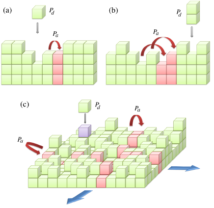
Figure 1: (Color online) Illustration of the substrate enlargement and deposition for (a) RSOS and (b) SS models in $1+1$ and in (c) $2+1$ dimensions.

The substrate enlargement is implemented as follows. A particle deposition is attempted with probability $P_{d}=N/(N+\omega d_{s})$ while a column duplication occurs with complementary probability $P_{a}=\omega d_{s}/(N+\omega d_{s})$, where $N$ is the number of the lattice sites and $d_{s}$ is the substrate dimension. After each event, time is increased by $\Delta t=1/(N+\omega d_{s})$. The initial lateral substrate size is $L_{0}$. In $d=1+1$, each substrate enlargement is implemented by a simple, local duplication of a randomly selected column for the RSOS and Etching models, as illustrated in Fig. 1(a). In $d=2+1$, a lattice row or column is randomly selected and similarly duplicated, as illustrated in Fig. 1(c). The lateral lattice size increases on average, therefore, as $\langle{L}\rangle=L_{0}+\omega t$. In the SS model, we must duplicate a pair of NN columns at once to conserve the steps at surface, see Fig. 1(b). Therefore, the substrate enlarging rate is $2\omega$.

Let us illustrate a consequence of the column duplication for the KPZ ansatz by an approximate argument. Let $\nabla h_{i}$ be the local gradient on a $d_{s}$-dimensional substrate, so that, $(\nabla h_{i})^{2}=\left(\frac{\partial h_{i}}{\partial x_{1}}\right)^{2}+\left(\frac{\partial h_{i}}{\partial x_{2}}\right)^{2}+\cdots+\left(\frac{\partial h_{i}}{\partial x_{d_{s}}}\right)^{2}$, where $x_{j}$ with $j=1,\cdots,d_{s}$ are the substrate directions. The mean squared gradient at time $t$ is

$$G_{t}=\frac{1}{L^{d_{s}}}\sum_{i=1}^{L^{d_{s}}}(\nabla h_{i})^{2}.$$

After $\omega$ duplications, in a time unity, we have

$$G_{t+1}=\frac{1}{(L+\omega)^{d_{s}}}\left[\sum_{i=1}^{L^{d_{s}}}(\nabla h_{i})^{2}+\sum_{i=1}^{(L+\omega)^{d_{s}}-L^{d_{s}}}(\nabla h_{i})^{2}\right],$$ (3)

where the first and second sums are taken over non-duplicated and duplicated sites, respectively. Considering only the effects of duplication and using the statistical equivalence of sites, we have

$$\sum_{i=1}^{L^{d_{s}}}(\nabla h_{i})^{2}\simeq L^{d_{s}}G_{t}$$

and

$$\sum_{i=1}^{(L+\omega)^{d_{s}}-L^{d_{s}}}(\nabla h_{i})^{2}\approx\frac{(d_{s}-1)}{d_{s}}\left[(L+\omega)^{d_{s}}-L^{d_{s}}\right]G_{t},$$

where the ratio $(d_{s}-1)/d_{s}$ appears because column duplication in direction $x_{k}$ implies $\left(\frac{\partial h_{i}}{\partial x_{k}}\right)^{2}=0$ along this column, right after the duplication. Inserting this result in Eq. (3) and considering long times, so that $L\sim\omega t$, we find

$$G_{t+1}\approx\left\{1+\frac{1}{d_{s}}\left[-1+\frac{1}{(1+1/t)^{d_{s}}}\right]\right\}G_{t}.$$

Therefore, disregarding terms $\mathcal{O}(t^{-2})$ for $t\gg 1$, we have

$$G_{t+1}-G_{t}\approx-\frac{1}{t}G_{t}\quad\quad\text{or}\quad\quad\frac{dG}{dt}\approx-\frac{1}{t}G,$$

implying $G_{t}\sim 1/t$ due to the substrate expansion. It is unclear whether the column duplication produces the same effect when the particle deposition is also considered, but the simplest scenario would be to assume that the above functional form of $G_{t}$ describes an additive correction to the height evolution (1), induced by the column duplication. This implies the presence of a logarithmic correction to the KPZ ansatz [Eq. (2)], which now reads

$$h\simeq v_{\infty}t+s_{\lambda}(\Gamma t)^{\beta}\chi+\eta+s_{\lambda}\zeta\ln t+\ldots$$ (4)

where $\zeta$ is, in principle, a stochastic variable. We will see that this logarithmic correction indeed exists in all models and dimensions we investigated, and that the fluctuations of $\zeta$, if exist, are very small. Note however that this logarithmic correction is predicted for the KPZ-class interfaces on expanding substrates and not necessarily for other universality classes. More importantly, one can easily see that the duplication of a column does not induce any curvature in the global scale, i.e.,

$$\langle{\nabla^{2}h}\rangle=0,$$

which is guaranteed here by the choice of the periodic boundary condition. This allows us to study the effect of the substrate expansion on the KPZ universal fluctuations, independently of the global curvature.

III Height fluctuations in $1+1$ dimensions

This section presents numerical results for the one-dimensional enlarging substrates, with $L_{0}=\omega$ and up to $25000$ realizations. Figure 2(a) shows the effective growth exponent, defined by $\beta_{\rm eff}(t)\equiv\frac{1}{2}\frac{d(\log\langle{h^{2}}\rangle_{c})}{d(\log t)}$ with the second-order cumulant $\langle{h^{2}}\rangle_{c}$, for all investigated models and two different values of $\omega$. The convergence to the expected KPZ value $\beta=1/3$ is found in all cases, in agreement with previous simulations of KPZ models in linearly growing domains, $L\sim t$ Pastor ; masoudi1 .

To characterize the asymptotic height distributions, we analyzed the dimensionless cumulant ratios $S=\left\langle h^{3}\right\rangle_{c}/\left\langle h^{2}\right\rangle_{c}^{3/2}$ (skewness) and $K=\left\langle h^{4}\right\rangle_{c}/\left\langle h^{2}\right\rangle_{c}^{2}$ (kurtosis), where $\left\langle h^{n}\right\rangle_{c}$ is the $n$th-order cumulant of $h$. The results are plotted in Fig. 2(b) as functions of $t^{-2\beta}$, which is an expected functional form for their finite-time correction, usually obtained on the basis of the correction of $\mathcal{O}(t^{-2\beta})$ in the second-order cumulant Oliveira12 ; Alves13 ; TakeuchiJSP ; Ferrari.Frings-JSP2011 . Our results indeed underpin this finite-time correction, and, extrapolating the data, we find that the asymptotic skewness and kurtosis indicate the values for the GUE TW distribution. We conclude, therefore, that the underlying distribution behind the asymptotic height fluctuations is given by the GUE TW distribution, rather than the GOE counterpart found for $\omega=0$. It is important to emphasize that the global curvature of the interface is not changed by duplications and remains identically null due to the periodic boundary conditions.

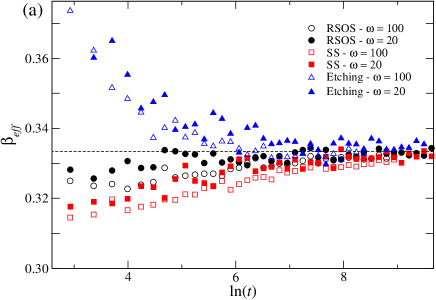
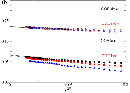
Figure 2: (Color online) (a) Effective growth exponent as a function of $\ln(t)$. (b) Skewness (open) and kurtosis (full symbols) of the height distributions for the RSOS (black circles), SS (red squares) and Etching (blue triangles) models, with $\omega=20$. Dashed and dotted horizontal lines indicate the expected values of $S$ and $K$ for the GUE and GOE TW distributions, respectively.

As $t\rightarrow\infty$, the number of the sites duplicated during each time unit becomes negligible compared with that of the non-duplicated sites. Therefore, the non-universal parameters such as $v_{\infty}$, $\lambda$ and $\Gamma$ should not be changed by the substrate expansion. This implies that it is sufficient for us to determine them for the non-expanding case, $\omega=0$. For the RSOS model, $v_{\infty}=0.419030(3)$ and $\Gamma=0.252(1)$ were numerically estimated in Oliveira12 ; Alves13 . The exact values of these quantities for the SS model are $v_{\infty}=\Gamma=1/2$ KrugPRA92 . Following the same procedures as in Refs. Oliveira12 ; TakeuchiJstat , we found $v_{\infty}=2.13986(5)$ and $\Gamma=4.90(9)$ for the Etching model. All these results were obtained for $\omega=0$, but the validity of these values for the expanding case was explicitly checked.

Accordingly to Eq. (2), we have

$$\partial_{t}\left\langle h\right\rangle\simeq v_{\infty}+s_{\lambda}\beta\Gamma^{\beta}\left\langle\chi\right\rangle t^{\beta-1}.$$

Then, plotting $\partial_{t}\left\langle h\right\rangle$ against $t^{\beta-1}$ should result in a straight line, whose $y$-intercept is $v_{\infty}$. However, we did not find such linear behavior even for the longest times investigated, as shown in Fig. 3(a). Indeed, the additional logarithmic correction predicted in Eq. (4) can not be neglected. Assuming that

$$\partial_{t}\left\langle h\right\rangle\simeq v_{\infty}+s_{\lambda}\beta\Gamma^{\beta}\left\langle\chi\right\rangle t^{\beta-1}+s_{\lambda}\langle{\zeta}\rangle t^{-\delta}+\ldots,$$ (5)

the correction $s_{\lambda}\langle{\zeta}\rangle t^{-\delta}$ can be obtained by plotting $C\equiv\partial_{t}\left\langle h\right\rangle-v_{\infty}-s_{\lambda}\beta\Gamma^{\beta}\left\langle\chi\right\rangle t^{\beta-1}$ against time, as shown in the inset of Fig. 3(a). For all investigated models, we found the exponent $\delta=1.01(1)$, consistent with the logarithmic correction, using $\left\langle\chi\right\rangle=\langle{\chi_{2}}\rangle$ (GUE TW). Instead, if the GOE TW value is used, $\delta\approx 1-\beta=2/3$ is found (see inset of Fig. 3(a)). This indicates that the term $t^{\beta-1}$ in Eq. (5) was not absorbed if the GOE TW value is assumed, giving further evidence that the GOE TW distribution does not correctly describe the distribution of $\chi$.

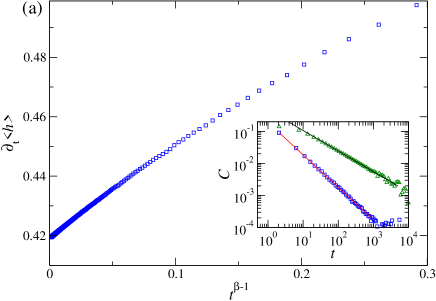
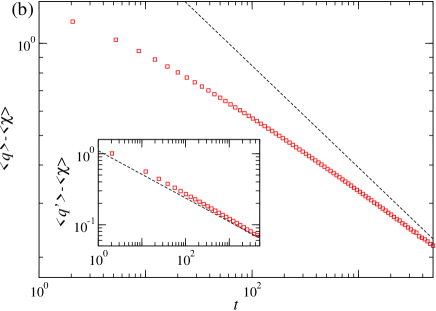
Figure 3: (Color online) (a) Growth velocity versus $t^{\beta-1}$. Inset shows $C\equiv\partial_{t}\left\langle h\right\rangle-v_{\infty}-s_{\lambda}\beta\Gamma^{\beta}\left\langle\chi\right\rangle t^{\beta-1}$ against $t$ with $\left\langle\chi\right\rangle=\left\langle\chi_{1}\right\rangle$ (green triangles) and $\left\langle\chi\right\rangle=\left\langle\chi_{2}\right\rangle$ (blue squares). The lines are results of power-law regressions. (b) Finite-time correction in the mean height versus time, disregarding (main plot) or considering (inset) the logarithmic correction (see text). Dashed lines indicate the slope $-1/3$. All data above were obtained for the RSOS model with $\omega=20$.

The importance of the logarithmic term in Eq. (4) is evidenced when we try to determine the usual finite-time correction term $\eta$. Defining the variable

$$q\equiv\frac{h-v_{\infty}t}{s_{\lambda}(\Gamma t)^{\beta}},$$

the finite-time correction in the mean height has a power law decay, $\left\langle q\right\rangle-\left\langle\chi\right\rangle\sim t^{-\beta}$, for $\omega=0$ Oliveira13 ; Alves13 ; TakeuchiPRL ; *TakeuchiSP; TakeuchiJSP ; Alves11 ; TakeuchiJstat ; Oliveira12 . However, for $\omega>0$, a power law decay is not found due to the logarithmic correction, as shown in Fig. 3(b). Instead, including the logarithm term as

$$q^{\prime}\equiv\frac{h-v_{\infty}t-s_{\lambda}\langle{\zeta}\rangle\ln t}{s_{\lambda}(\Gamma t)^{\beta}},$$ (6)

and using the value of $\langle{\zeta}\rangle$ estimated from the power law regressions shown in the inset of Fig.3(a), the finite-time correction decaying as $t^{-\beta}$ is recovered (see inset of Fig. 3(b)). Moreover, we observe that $\langle{\zeta}\rangle$ does not significantly depend on $\omega$ and take values $\langle{\zeta}\rangle=0.18(1)$, $0.15(4)$ and $0.22(3)$ for the RSOS, SS and Etching models, respectively, for $\omega$ varying from $1$ to $100$. Our analysis does not permit a conclusive assessment on logarithmic corrections in higher-order cumulants of the height distribution. For SS model, for which $\Gamma=1/2$ is exactly known, $\langle{h^{n}}\rangle_{c}-[s_{\lambda}(\Gamma t)^{\beta}]^{n}\langle{\chi^{n}}\rangle_{c}$ seems to reach a constant value, suggesting that $\zeta$ is deterministic. For RSOS, a very small variance $\langle{\zeta^{2}}\rangle_{c}\approx 0.005$, smaller than the uncertainties obtained with our current precision in $\Gamma$, is found.

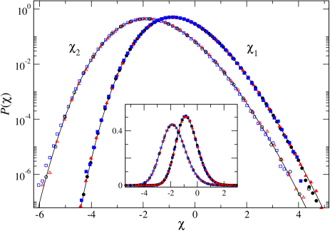
Figure 4: (Color online) Rescaled height distributions for the RSOS (black circles), SS (red triangles) and Etching (blue squares) models, with $\omega=20$ (open symbols) for times $t=18000$, 19000 and 15000, respectively, and with $\omega=0$ (full symbols) for $t=2000$, 2000 and 1500, respectively. Main plot and inset show these data in semi-log and linear scales, respectively. Here, histograms of $\chi\equiv(h-v_{\infty}t-\langle{\eta}\rangle-s_{\lambda}\zeta\ln t)/(\Gamma t)^{\beta}$ are compared with the probability density of $\chi_{1}$ and $\chi_{2}$.

Similarly to $\langle{\zeta}\rangle$, $\langle{\eta}\rangle$ also seems to be independent of $\omega$: we found $\langle{\eta}\rangle=-0.87(3)$, -0.44(3) and 3.2(2) for the RSOS, SS and Etching models, respectively, for the values of $\omega$ we investigated ($\omega\geq 1$). However, they are larger (in the absolute value) than the estimates for $\omega=0$, which are $\langle{\eta}\rangle=-0.32(4)$ for the RSOS model Alves13 , and $\langle{\eta}\rangle=-0.33(1)$ for the SS and $\langle{\eta}\rangle=0.20(3)$ for the Etching models (present work). Note that, for short times, the surface roughness is very small and duplication of columns does not have significant effects on the mean height, so that $\left\langle h\right\rangle_{\omega>0}\approx\left\langle h\right\rangle_{\omega=0}$ for short times. This suggests that $\langle{\eta}\rangle$ becomes larger for $\omega>0$ so as to compensate the change in the mean height due to the crossover from the GOE TW distribution to the GUE counterpart (see Sec. VII).

Height distributions rescaled according to Eq. (4) are presented in Fig. 4. Excellent data collapse with the theoretical curve for the GUE TW distribution demonstrates that the asymptotic height fluctuations of flat models on the growing substrates are given by the GUE TW distribution. The distributions for the same models with $\omega=0$ are also shown for the sake of comparison. It is important to remark that rescaled height distributions without taking into account the logarithmic correction display a shift in the mean decaying very slowly as $\ln(t)/t^{\beta}$.

IV Height fluctuations in $2+1$ dimensions

For two-dimensional enlarging substrates, we used $L_{0}=\omega$ in both directions, with $\omega$ varied from $1$ to $10$, and averages were taken over $40000$ samples.

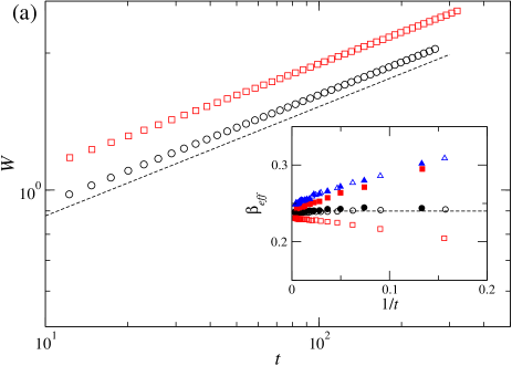
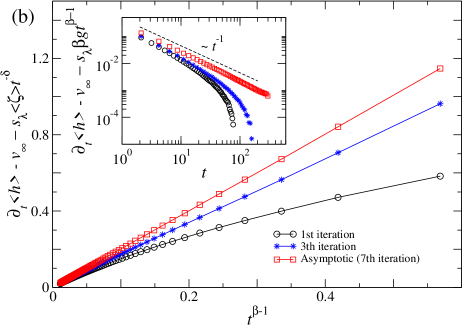
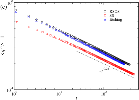
Figure 5: (Color online) (a) Interface width versus time for the RSOS (black circles) and SS (red squares) models, with $\omega=10$. Inset shows the effective growth exponents for the RSOS, SS and Etching (blue triangles) models, with $\omega=6$ (full) and $10$ (open symbols). Dashed line has the slope $\beta=0.24$. (b) Illustration of the method to self-consistently determine $g\equiv\Gamma^{\beta}\langle{\chi}\rangle$ (main plot) and $\langle{\zeta}\rangle t^{-\delta}$ (inset) for the RSOS model with $\omega=6$. We start the first iteration with $\langle{\zeta}\rangle t^{-\delta}=0$. (c) Shift in rescaled mean height versus time for the three models with $\omega=6$.

Figure 5(a) shows the interface width ($W\equiv\sqrt{\left\langle h^{2}\right\rangle_{c}}$) evolution in time and the corresponding effective growth exponent. Analogously to the one-dimensional case, the growth exponent values converge to that of the KPZ class in $d=2+1$ dimensions, $\beta\approx 0.24$ Kelling . The asymptotic growth velocities $v_{\infty}$ for the three models with $\omega=0$ were calculated in Oliveira13 (see Table I). For $\omega>0$, we find behavior of $\partial_{t}\left\langle h\right\rangle$ analogous to that for $d=1+1$ (Fig. 3(a)), but since here the exact value of $\langle{\chi}\rangle$ is not known, we determine $\langle{\zeta}\rangle$ and $\delta$ in Eq. (5) in an iterative way as follows. Plotting $\partial_{t}\left\langle h\right\rangle-v_{\infty}$ against $t^{\beta-1}$, we estimate a rough value for the product $g\equiv\Gamma^{\beta}\langle{\chi}\rangle$ from the slope near the origin (Fig. 5(b)). We then use this approximate value to plot $\partial_{t}\left\langle h\right\rangle-v_{\infty}-s_{\lambda}\beta gt^{\beta-1}$ against $t$ in logarithmic scales (inset of Fig. 5(b)) as done in Fig. 3(a). We expect it to decay as $\langle{\zeta}\rangle t^{-\delta}$ with $\delta>1-\beta$, but because of the error in the estimate of $g$, the residual in the order of $t^{\beta-1}$ dominates for large $t$. Therefore, $\langle{\zeta}\rangle$ and $\delta$ can be estimated from the data at small $t$. With these estimates, we reestimate $g$ by plotting $\partial_{t}\left\langle h\right\rangle-v_{\infty}-s_{\lambda}\langle{\zeta}\rangle t^{-\delta}$ against $t^{\beta-1}$ (see again the main panel of Fig. 5(b)). Repeating this procedure to improve the estimates $g,\langle{\zeta}\rangle,\delta$ until they reach some asymptotic values, we finally find straight lines in both plots (red squares), which guarantee the self-consistency of the estimates. In particular, we find $\delta\approx 1$ which indicates the presence of a logarithmic correction in the KPZ ansatz also for $d=2+1$, as expected by the theoretical argument presented in Sec. II. As in $d=1+1$, $\langle{\zeta}\rangle$ is almost independent of $\omega$ within the range of $\omega$ studied here, taking values at $\langle{\zeta}\rangle=0.32(2),0.36(4),0.39(2)$ for the RSOS, SS and Etching models, respectively.

To determine $\langle{\eta}\rangle$, following Refs. Alves13 ; Oliveira13 , we define the variable

$$q^{\prime\prime}\equiv\frac{h-v_{\infty}t-s_{\lambda}\langle{\zeta}\rangle\ln t}{s_{\lambda}gt^{\beta}},$$ (7)

so that $\langle{q^{\prime\prime}}\rangle-1\simeq(s_{\lambda}\langle{\eta}\rangle/g)t^{-\beta}$. Figure 5(c) shows this shift against time, where the expected decay $t^{-\beta}$ is observed and, using the values of $g$ obtained above, we estimate $\langle{\eta}\rangle$ at $\left\langle\eta\right\rangle=-1.8(2)$, -1.4(1), and 4.9(1) for the RSOS, SS and Etching models, respectively. These values are again independent of $\omega$ within $1\leq\omega\leq 10$ and larger than the values for $\omega=0$ (see Table I in Ref. Oliveira13 ).

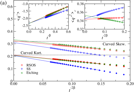
Figure 6: (Color online) (a) Skewness (open) and kurtosis (full symbols) against $t^{-2\beta}$ for all investigated models with $\omega=10$. Insets show $\langle{q^{\prime}}\rangle$ (left) and $\langle{q^{\prime 2}}\rangle_{c}$ (right) versus $t^{-\beta}$ and $t^{-2\beta}$, respectively, for the same models. (b) Rescaled height distributions for RSOS, SS and Etching models, with $\omega=4$ (open symbols) and times $t=500$, 650 and 350, respectively, and, with $\omega=0$ (full symbols) and $t=10000$, 8000 and 2000, respectively. Main panel and inset show these data in semi-log and linear scales, respectively. Full lines are generalized Gumbel distributions with $m=9.5$ (left) and $m=6.0$ (right) Oliveira13 .

The parameter $\Gamma$ is given by $\Gamma=(1/2)|\lambda|A^{1/\alpha}=|\lambda|A^{2}/2$ for $d=1+1$ dimensions and $\Gamma=|\lambda|A^{1/\alpha}$ for $d=2+1$ dimensions, where $A$ is defined by the steady-state growth velocity $v_{s}(L)$ in a system of (fixed) size $L$, through $v_{s}(L)-v_{s}(\infty)=-(\lambda A/2)L^{2\alpha-2}$ Krug90 ; KrugPRA92 ; healy2014 . Note that the presence or absence of the factor 1/2 in the above expressions for $\Gamma$ is not essential, but introduced only to conform with the definitions adopted in past studies. The parameter $\lambda$ can be obtained from the dependence of the asymptotic growth velocity on the substrate slope $u$ Krug90 ; specifically, $\lambda=\left(\frac{\partial^{2}v_{\infty}}{\partial u^{2}}\right)_{u\rightarrow 0}$. Therefore, by plotting $v_{s}(L)-v_{s}(\infty)$ against $L^{2\alpha-2}$ with the value $\alpha=0.39$ for the (2+1)-dimensional KPZ class marinari ; Kelling , and by using all the expressions above, we determined $A$ and $\Gamma$ as listed in Table I.

		$v_{\infty}$ Oliveira13		$\lambda$		$A$		$\Gamma$		$\langle\chi\rangle_{c}$		$\langle\chi^{2}\rangle_{c}$		$S$		$K$
RSOS		0.31270(1)		-0.405(7)		1.22(4)		0.68(6)		-2.34(3)		0.341(5)		0.328(4)		0.210(4)
SS		0.341368(3)		-0.481(3)		1.44(5)		1.2(1)		-2.37(5)		0.336(6)		0.329(7)		0.206(3)
Etching		3.3340(1)		2.147(4)		3.629(9)		58.5(5)		-2.36(3)		0.346(8)		0.336(6)		0.21(1)

Table 1: Non-universal ($v_{\infty}$, $\lambda$, $A$ and $\Gamma$) and universal ($\langle\chi\rangle_{c}$, $\langle\chi^{2}\rangle_{c}$, $S$ and $K$) quantities for different models on enlarging $d=2+1$ dimensional substrates. The averages and uncertainties of universal quantities were determined using different substrate expansion rates $\omega>0$.

Using the estimated parameter values to rescale the height as in Eq. (6), universality in the height distribution for $d=2+1$ can be explicitly assessed. The mean and the variance of $\chi$ are obtained from extrapolations of $\left\langle q^{\prime}\right\rangle$ and $\left\langle q^{\prime 2}\right\rangle_{c}$ against $t^{-\beta}$ and $t^{-2\beta}$, respectively, as shown in the insets of Fig. 6(a). Table I summarizes the values obtained by using different substrate expansion rates $\omega>0$. These values are in good agreement with those obtained by Halpin-Healy healy12 ; healy13 for curved interfaces and far from those for the flat ones. Therefore, the underlying fluctuations in two-dimensional enlarging substrates are also equivalent to those found for curved systems. This is corroborated by the skewness and the kurtosis of the height distributions, which converge to the corresponding values for the curved interfaces, as shown in Fig. 6(a) and Table I. It is worth stressing again that the global curvature of the interfaces is identically null as in $d=1+1$.

Finally, the height distributions rescaled according to Eq. (4) are shown in Fig. 6(b), where the excellent data collapse gives another evidence for their universality. Figure 6(b) also shows the generalized Gumbel distribution with parameter $m=9.5$ (with $S=0.332$ and $K=0.221$ and rescaled to mean $-2.33$ and variance $0.34$ noteGumbel ), which is a good fit of $\chi$ for the curved KPZ subclass in $d=2+1$ Oliveira13 . Moreover, rescaled distributions for $\omega=0$ are also shown in Fig. 6(b), which clearly show the existence of two different universal distributions for the underlying fluctuations of fixed-size and enlarging substrate KPZ subclasses in $d=2+1$. Again, the generalized Gumbel distribution, with parameter $m=6.0$ (with $S=0.424$ and $K=0.359$ and rescaled to mean $-0.90$ and variance $0.24$ noteGumbel ), provides a good fit of $\chi$ for almost five decades around the peak, as also observed in Oliveira13 .

V Spatial covariance

Beyond the asymptotic height distribution, the limiting processes that describe the spatial profile of the flat and curved KPZ-class interfaces are exactly known in 1+1 dimensions and called the Airy₁ and Airy₂ processes, respectively PraSpo3 ; *Sasa2005; *Borodin; Kriecherbauer.Krug-JPA2010 . We calculate the spatial covariance

$$C_{s}(r,t)=\left\langle\tilde{h}(x,t)\tilde{h}(x+r,t)\right\rangle\simeq(\Gamma t)^{2\beta}\Psi[A_{h}r/(\Gamma t)^{2\beta}],$$ (8)

where $\tilde{h}\equiv h-\left\langle h\right\rangle$, $\Psi$ is a scaling function and $A_{h}=A$ in $1+1$ and $A_{h}=0.6460A$ in $2+1$ dimensions healy2014 . Figure 7(a) shows the rescaled spatial covariance for $d=1+1$ along with the Airy₁ and Airy₂ covariances. We find that the results for $\omega>0$ and $\omega=0$ are in good agreement with the Airy₂ and Airy₁ covariances, respectively, showing that the equivalence between expanding substrate systems and curved interfaces also holds for the spatial correlation.

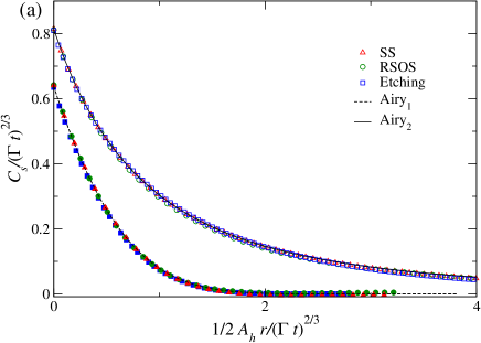
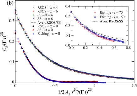
Figure 7: (Color online) (a) Rescaled spatial covariances for all investigated models in $d=1+1$ with $\omega=0$ (full) and $\omega=20$ (open symbols), for times $t=4000$ and 10000, respectively. (b) Rescaled spatial covariances in $d=2+1$ dimensions, for times $t=600$ ($\omega=0$), $t=250$ ($\omega=4$) and $t=150$ ($\omega=6$). Results for the Etching model on enlarging substrates are shown in the inset at two different times. Exponents $\alpha=0.395$ and $\beta=0.237$ were used for the rescaling.

In $d=2+1$, the spatial covariance for flat interfaces was numerically calculated only very recently healy2014 and it was shown to be universal, as is the case for $d=1+1$. However, there were no reports on the spatial covariance for curved interfaces up to the present work. Here, we determined the spatial covariance for the investigated models for both $\omega=0$ and $\omega>0$. The rescaled curves are presented in Fig. 7(b), where two universal curves for fixed-size and enlarging substrates are observed. These can be regarded as the (2+1)-dimensional analogue of the Airy₁ and Airy₂ covariances, respectively. For the Etching model on enlarging substrates, the rescaled curves do not converge yet within the examined time window, but are still approaching the asymptotic curve obtained for the RSOS and SS models (see inset of Fig. 7).

VI Temporal covariance

Similarly to the spatial case, we can define the temporal covariance

$$C_{t}(t,t_{0})=\left\langle\tilde{h}(x,t_{0})\tilde{h}(x,t)\right\rangle,$$ (9)

which is expected to scale as $C_{t}(t,t_{0})\simeq(\Gamma^{2}t_{0}t)^{\beta}\Phi(t/t_{0})$ Kallabis99 ; Singha-JSM2005 ; TakeuchiJSP . Similarly to the results for the spatial correlation, it is reasonable to expect that the scaling function $\Phi(x)$ is universal within each subclass and dimensionality. However, unlike the spatial correlation, no exact results have been obtained for the temporal correlation, even for $d=1+1$. Therefore, it is very important to check their universality by empirical approaches, such as simulations and experiments.

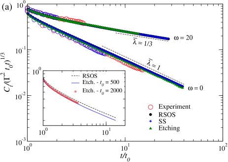
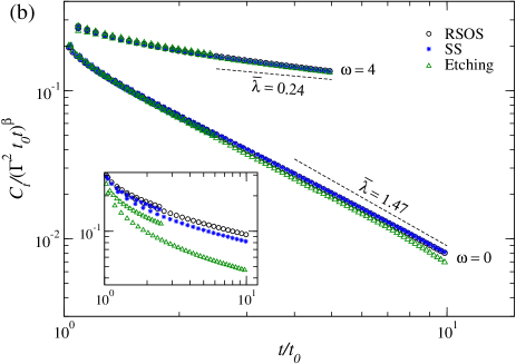
Figure 8: (Color online) (a) Rescaled temporal covariance for all investigated models (full symbols) in $d=1+1$ and the liquid-crystal experiment (open symbols) with flat and curved interfaces. In both cases, different initial times $t_{0}$ in the range $[100,2000]$ (models) and $[4s,25s]$ (experiment) were used. For Etching model and curved experimental surfaces, the curves are extrapolations. The raw data for Etching model are shown in the inset. (b) Rescaled temporal covariances for all models in $d=2+1$ dimensions and different initial times. For $\omega=4$, all curves in the main panel are extrapolations, while the non-extrapolated ones are shown in the inset.

Figure 8(a) shows the rescaled temporal covariance for all investigated models in $d=1+1$ on fixed-size and enlarging substrates, along with the experimental data for flat and curved interfaces, respectively, generated in the electroconvection of nematic liquid crystals TakeuchiPRL ; *TakeuchiSP; TakeuchiJSP (already reported in TakeuchiJSP ). For fixed-size substrates, a good collapse of data for all models and initial times $t_{0}$ is observed. Moreover, a good agreement between the numerical and experimental covariances is also found. For enlarging substrates, the temporal covariances for the RSOS and SS models already reach an asymptotic function, clearly different from that for the fixed-size case, while finite-time effect seems to be more severe for the Etching model, similarly to the spatial covariance as reported in the inset of Fig. 7(b). Similar effect was also observed for the curved interfaces in the liquid-crystal experiment (see the inset of Fig. 11(b) in Ref. TakeuchiJSP ).

To substantiate that the deviation from the asymptotic form is indeed a finite-time effect, we attempt an extrapolation of the finite-time data as follows. Assuming that $\eta$ is stochastic (as shown by past studies Oliveira12 ; Alves13 ; TakeuchiJSP ; Ferrari.Frings-JSP2011 ) and neglecting $\zeta$ fluctuations (as discussed above), we expect from the KPZ ansatz [Eq. (4)] that the leading correction in $\Phi$ is in the order of $t^{-\beta}$. Using this expression and data at two different $t_{0}$ with fixed $t/t_{0}$, we can extrapolate to obtain the asymptotic temporal covariance $\Phi$. The data for the Etching model in the main panel of Fig. 8(a) are obtained in this way from the raw data in the inset, and an excellent agreement with the raw data for the RSOS and SS models is achieved. For the experimental data of the curved interfaces, the same quality of the collapse and agreement is obtained, by assuming that the leading finite-time correction to $\Phi$ is $\mathcal{O}(t_{0}^{-2\beta})$. This may be related to the vanishing finite-time correction for the one-point second-order cumulant $\langle{\chi^{2}}\rangle_{c}$ for the curved case TakeuchiJSP , but such relationship needs to be clarified by further analytical and empirical studies.

In $d=2+1$, for fixed-size substrates, we again find a good collapse of rescaled (non-extrapolated) temporal covariances for all models and initial times, as shown in Fig. 8(b). However, for enlarging systems the finite-time effects are larger and, even for the RSOS and SS models we do not attain a data collapse, as shown in the inset of Fig. 8(b). In these models, extrapolations for the correction $\mathcal{O}(t_{0}^{-\beta})$ fail to collapse the data, whereas a correction $\mathcal{O}(t_{0}^{-2\beta})$ provides a nice collapse for both models and for different times used for the extrapolation (Fig. 8(b)). For the Etching model, a good collapse of data is not achieved with corrections $\mathcal{O}(t_{0}^{-\beta})$ or $\mathcal{O}(t_{0}^{-2\beta})$. Instead, an apparent collapse is achieved with an intermediate exponent $\mathcal{O}(t_{0}^{-0.32})$, possibly arising from a mixture of both terms above, within the time window we investigated.

The strengths of the two correction terms, $\mathcal{O}(t_{0}^{-\beta})$ and $\mathcal{O}(t_{0}^{-2\beta})$, may be related to the finite-time correction to the second-order cumulant $\langle{\chi^{2}}\rangle_{c}$. Indeed, the Etching model, whose correction to the second-order cumulant is known to be large FabioSS , also exhibits the large finite-time corrections to the temporal covariance, as presented above. Although these two corrections are formally different as they concern equal-time and two-time properties, respectively, better understanding of such relationship will certainly serve for a more unambiguous determination of the universal functional forms for the temporal covariance.

In any case, our results in Fig. 8 show that the temporal covariance is clearly different between the fixed-size and enlarging systems, and that they agree, in $d=1+1$ dimensions, with the results for the flat and curved interfaces in the liquid-crystal experiment, respectively. The rescaled covariance $\Phi(t/t_{0})$ converges to a universal function in each case and each dimensionality, as substantiated by the three models investigated here. Importantly, Kallabis and Krug Kallabis99 had conjectured that for long times $\Phi(x)\sim x^{-\bar{\lambda}}$ with $\bar{\lambda}=\beta+d_{s}/z$ for the flat interfaces, while $\bar{\lambda}=\beta$ was later proposed for the curved interfaces Singha-JSM2005 . Besides confirming these scaling relations in $d=1+1$, our results suggest that they also seem to be valid for $d=2+1$ (dashed lines in Fig. 8(b)), though clear power laws are not yet reached within the time studied.

VII Crossover from fixed-size to enlarging substrates

Our enlarging-substrate systems are also convenient to study crossover between the fixed-size/flat and enlarging/curved subclasses, or, for $1+1$ dimensions, between the GOE and GUE TW distributions. Such inter-subclass crossover has also attracted great interest Corwin-RMTA2012 , both theoretically and experimentally. Analytical studies have mostly dealt with crossover in space for $1+1$ dimensions Corwin-RMTA2012 : for example, Borodin et al. Borodin.etal-CPAM2008 and Le Doussal ledoussal considered an initial condition composed of a flat substrate for $x<0$ and a wedge (curved) one for $x>0$, and formulated crossover from the GOE to GUE TW distributions, or from the Airy₁ to Airy₂ processes, which takes place as one moves from $x\to-\infty$ to $x\to\infty$. In contrast, crossover in time remains out of the reach of analytical studies, as it requires understanding of the temporal covariance, but it has been recently addressed numerically and experimentally, for the crossover from the flat to stationary subclasses TakeuchiCross ; HealyCross ; healy13 . Here, we investigate temporal crossover from the fixed-size/flat to the enlarging/curved subclasses (from GOE to GUE TW for $d=1+1$), by starting with an initial substrate such that $L_{0}\gg\omega$. As the mean substrate size grows as $\langle{L}\rangle=L_{0}+\omega t$, the characteristic crossover time is given by $t^{*}\sim L_{0}/\omega$. We therefore expect that, for $t\ll t^{*}$ (or equivalently $\omega\rightarrow 0$ or $L_{0}\rightarrow\infty$), the system essentially behaves as a fixed-size system, while for $t\gg t^{*}$ the statistical properties of the enlarging/curved systems should take over.

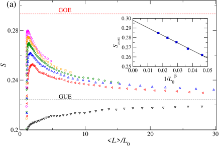
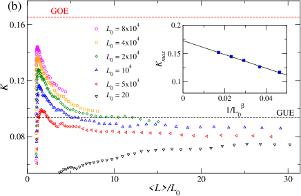
Figure 9: (Color online) Evolution of (a) the absolute value of the skewness and (b) the kurtosis for the one-dimensional RSOS model with $\omega=20$ and different initial system sizes. Insets show the maximal values against $L_{0}^{-\beta}$, with linear extrapolations to the asymptotic values.

This scenario is indeed consistent with our results shown in Figs. 9(a) and 9(b), where the skewness $S$ and kurtosis $K$ of the one-dimensional RSOS model are plotted as functions of $\langle{L}\rangle/L_{0}\simeq t/t^{*}$. The cumulant ratios reach maxima near $t=t^{*}$, at some values close to those for the GOE TW distribution, and then approach the GUE TW values. As expected, the larger $L_{0}$ becomes, the closer the maximal values of the cumulant ratios are to the GOE TW values. Interestingly, these maxima $S_{\rm max}(L_{0})$ and $K_{\rm max}(L_{0})$ are found to vary linearly with $L_{0}^{-\beta}$ (insets). This allows us to extrapolate the asymptotic values $S_{\rm max}(\infty)=0.297(4)$ and $K_{\rm max}(\infty)=0.17(1)$, which agree with the GOE TW distribution ($S=0.2935,K=0.1652$). Similar results were also obtained for all models in $2+1$ dimensions (data not shown).

VIII Conclusions

In this article, we studied typical models of the KPZ class, on flat substrates enlarging at a constant rate $\omega$. While the growth exponent $\beta$ is the same for fixed-size ($\omega=0$) and enlarging ($\omega>0$) substrates, the height distribution does change: for the fixed-size case, it is given by the universal distribution for the flat interfaces (GOE TW in $d=1+1$), while for the enlarging case the distribution for the curved interfaces arises (GUE TW in $d=1+1$). We also reached the same conclusion for the spatial and temporal covariances. In particular, we found the Airy₁ and Airy₂ covariance for the spatial correlation of the fixed-size and enlarging systems in $d=1+1$, respectively, as well as agreement with the Kallabis-Krug conjecture on the temporal covariance Kallabis99 ; Singha-JSM2005 ; TakeuchiJSP . Moreover, we also studied $(2+1)$-dimensional systems and found clear agreement in the height distribution, with the functional forms previously obtained numerically for the curved and flat interfaces.

All these results indicate that the interfaces growing on enlarging substrates share the same statistical properties as the curved interfaces, despite the fact that the global curvature in these enlarging systems is kept exactly null. This suggests that the substrate enlargement is possibly more relevant for the realization of the “curved interface” subclass than the global curvature itself. Indeed, to our knowledge, all interfaces deemed “curved” in previous work (e.g., Kriecherbauer.Krug-JPA2010 ; Corwin-RMTA2012 ; Johansson-CMP2000 ; PraSpo1 ; Tracy.Widom-CMP2009 ; TakeuchiSP ; TakeuchiJSP ; SasaSpo1 ; Oliveira13 ) evolve within a zone of activity that grows linearly in time. The activity zone corresponds to the growing circumference for the usual circular interfaces, but this concept is also valid for the ASEP with the step initial condition Johansson-CMP2000 ; Tracy.Widom-CMP2009 , in which particles can move only within a linearly growing area around the origin. We hope that the relevance of such substrate enlargement to the “curved interface” subclass will be further investigated on a mathematical or theoretical basis; for this, the so-called characteristic lines Ferrari-JSM2008 ; Corwin.etal-AIHPBPS2012 may be a useful concept, which describe the directions of the fluctuation propagation in space-time.

Beyond those asymptotic universal quantities, finite-time behavior was also characterized. We found a logarithmic correction in the height evolution [Eq. (4)] when the substrate is enlarging. We consider that this correction is a consequence of column duplications adopted in our time evolution rule for enlarging substrates. Furthermore, crossover from the fixed-size (flat) to the enlarging substrate (curved) subclasses (GOE to GUE TW distributions in $d=1+1$), which takes place in the course of time evolution, has also been characterized.

As a final remark, we stress that our simulation method based on the substrate enlargement provides a powerful tool to study statistical properties of the curved interface subclass, since this produces isotropic interfaces on a lattice. This is not the case of the usual growth models on lattice, such as the Eden model, which is known to produce an anisotropic interface even from a single point seed Stauffer86 ; Paiva07 ; Alves13 reflecting the lattice structure of the model. Having access to isotropic interfaces instead is essential to study statistical properties of interest numerically, because then we can use all spatial points to improve statistics and to define the spatial correlation functions unambiguously. Indeed, in this article, this allowed us to determine the two-point spatial correlation function for the enlarging/curved systems in $2+1$ dimensions, for the first time, numerically. Our method of enlarging substrates therefore provides a useful platform to study statistical properties of the KPZ class in higher dimensions, and of other universality classes for fluctuating surface growth problems.

- (1) A.-L. Barabasi and H. E. Stanley, Fractal Concepts in Surface Growth (Cambridge University Press, Cambridge, England, 1995)
- (2) P. Meakin, Fractals, Scaling and Growth far from Equilibrium (Cambridge University Press, Cambridge, England, 1998)
- (3) J. W. Evans, P. A. Thiel, and M. Bartelt, Surf. Sci. Rep. 61, 1 (2006)
- (4) A. Pimpinelli and J. Villain, Physics of Crystal Growth (Cambridge University Press, Cambridge, England, 1998)
- (5) T. Vicsek, M. Cserzö, and V. K. Horváth, Physica A 167, 315 (1990)
- (6) A. Brú, J. M. Pastor, I. Fernaud, I. Brú, S. Melle, and C. Berenguer, Phys. Rev. Lett. 81, 4008 (1998)
- (7) J. Galeano, J. Buceta, K. Juarez, B. P. no, J. de la Torre, and J. M. Iriondo, Europhys. Lett. 63, 83 (2003)
- (8) M. A. C. Huergo, M. A. Pasquale, P. H. González, A. E. Bolzán, and A. J. Arvia, Phys. Rev. E 85, 011918 (Jan 2012)
- (9) K. A. Takeuchi and M. Sano, Phys. Rev. Lett. 104, 230601 (2010)
- (10) K. A. Takeuchi, M. Sano, T. Sasamoto, and H. Spohn, Sci. Rep. 1, 34 (2011)
- (11) K. Takeuchi and M. Sano, J. Stat. Phys. 147, 853 (2012)
- (12) P. J. Yunker, M. A. Lohr, T. Still, A. Borodin, D. J. Durian, and A. G. Yodh, Phys. Rev. Lett. 110, 035501 (2013)
- (13) J. Krug, Phys. Rev. Lett. 102, 139601 (2009)
- (14) A. A. Masoudi, S. Hosseinabadi, J. Davoudi, M. Khorrami, and M. Kohandel, J. Stast. Mech.: Theor. Exp. 2012, L02001 (2012)
- (15) A. A. Masoudi, M. Khorrami, M. Stastna, and M. Kohandel, Europhys. Lett. 100, 16004 (2012)
- (16) S. C. Ferreira and S. G. Alves, J. Stat. Mech.: Theor. Exp. 2006, P11007 (2006)
- (17) M. Prähofer and H. Spohn, Phys. Rev. Lett. 84, 4882 (2000)
- (18) T. Kriecherbauer and J. Krug, J. Phys. A 43, 403001 (2010)
- (19) I. Corwin, Random Matrices Theory Appl. 1, 1130001 (2012)
- (20) S. G. Alves, T. J. Oliveira, and S. C. Ferreira, J. Stat. Mech.: Theor. Exp. 2013, P05007 (2013)
- (21) C. Tracy and H. Widom, Commun. Math. Phys. 159, 151 (1994)
- (22) M. Kardar, G. Parisi, and Y.-C. Zhang, Phys. Rev. Lett. 56, 889 (1986)
- (23) S. G. Alves, T. J. Oliveira, and S. C. Ferreira, Europhys. Lett. 96, 48003 (2011)
- (24) K. A. Takeuchi, J. Stat. Mech. 2012, P05007 (2012)
- (25) T. J. Oliveira, S. C. Ferreira, and S. G. Alves, Phys. Rev. E 85, 010601 (2012)
- (26) T. Sasamoto and H. Spohn, Phys. Rev. Lett. 104, 230602 (2010)
- (27) G. Amir, I. Corwin, and J. Quastel, Commun. Pure Appl. Math. 64, 466 (2011)
- (28) P. Calabrese and P. Le Doussal, Phys. Rev. Lett. 106, 250603 (2011)
- (29) T. Imamura and T. Sasamoto, Phys. Rev. Lett. 108, 190603 (2012)
- (30) T. Halpin-Healy, Phys. Rev. Lett. 109, 170602 (2012)
- (31) T. Halpin-Healy, Phys. Rev. E 88, 042118 (2013)
- (32) T. J. Oliveira, S. G. Alves, and S. C. Ferreira, Phys. Rev. E 87, 040102 (2013)
- (33) R. A. L. Almeida, S. O. Ferreira, T. J. Oliveira, and F. D. A. Aarão Reis, Phys. Rev. B 89, 045309 (2014)
- (34) T. Halpin-Healy and G. Palasantzas, Europhys. Lett. 105, 50001 (2014)
- (35) S. G. Alves, T. J. Oliveira, and S. C. Ferreira, Phys. Rev. E 90, 020103(R) (2014)
- (36) J. M. Pastor and J. Galeano, Cent. Eur. J. Phys 5, 539 (2007)
- (37) C. Escudero, J. Stat. Mech. 2009, P07020 (2009)
- (38) J. M. Kim and J. M. Kosterlitz, Phys. Rev. Lett. 62, 2289 (1989)
- (39) B. A. Mello, A. S. Chaves, and F. A. Oliveira, Phys. Rev. E 63, 041113 (2001)
- (40) P. L. Ferrari and R. Frings, J. Stat. Phys. 144, 1123 (2011), ISSN 0022-4715
- (41) J. Krug, P. Meakin, and T. Halpin-Healy, Phys. Rev. A 45, 638 (1992)
- (42) J. Kelling and G. Ódor, Phys. Rev. E 84, 061150 (2011)
- (43) J. Krug and P. Meakin, J. Phys. A: Math. Gen. 23, L987 (1990)
- (44) E. Marinari, A. Pagnani, and G. Parisi, J. Phys. A: Math. Gen. 33, 8181 (2000)
- (45) Although the generalized Gumbel distributions with and serve as good fits to the distribution for the flat and curved KPZ subclasses, respectively, in dimensions Oliveira13 , no theoretical argument suggests that they are the true asymptotic distributions. Therefore, the values of their skewness and kurtosis are not exactly those for the KPZ class. For the KPZ class values, one should refer to numerical estimates, reported in healy12 ; healy13 ; Oliveira13
- (46) M. Prähofer and H. Spohn, J. Stat. Phys. 108, 1071 (2002)
- (47) T. Sasamoto, J. Phys. A: Math. Theor. 38, L549 (2005)
- (48) A. Borodin, P. Ferrari, and T. Sasamoto, Commun. Math. Phys. 283, 417 (2008)
- (49) H. Kallabis and J. Krug, Europhys. Lett. 45, 20 (1999)
- (50) S. B. Singha, J. Stat. Mech. 2005, P08006 (2005)
- (51) F. D. A. Aarão Reis, Phys. Rev. E 69, 021610 (2004)
- (52) A. Borodin, P. L. Ferrari, and T. Sasamoto, Commun. Pure Appl. Math. 61, 1603 (2008), ISSN 1097-0312
- (53) P. Le Doussal, J. Stat. Mech. 2014, P04018 (2014)
- (54) K. A. Takeuchi, Phys. Rev. Lett. 110, 210604 (2013)
- (55) T. Halpin-Healy and Y. Lin, Phys. Rev. E 89, 010103 (2014)
- (56) K. Johansson, Commun. Math. Phys. 209, 437 (Feb. 2000)
- (57) C. A. Tracy and H. Widom, Commun. Math. Phys. 290, 129 (2009), ISSN 0010-3616
- (58) P. L. Ferrari, J. Stat. Mech. 2008, P07022 (2008)
- (59) I. Corwin, P. L. Ferrari, and S. Péché, Ann. Inst. H. Poincaré B Probab. Statist. 48, 134 (2012)
- (60) J. G. Zabolitzky and D. Stauffer, Phys. Rev. A 34, 1523 (1986)
- (61) L. R. Paiva and S. C. Ferreira, J. Phys. A: Math. Theor. 40, F43 (2007)