Abstract

This is a survey of results on long time behavior and attractors for nonlinear Hamiltonian partial differential equations, considering the global attraction to stationary states, stationary orbits, and solitons, the adiabatic effective dynamics of the solitons, and the asymptotic stability of the solitary manifolds. The corresponding numerical results and relations to quantum postulates are considered.

This theory differs significantly from the theory of attractors of dissipative systems where the attraction to stationary states is due to an energy dissipation caused by a friction. For the Hamilton equations the friction and energy dissipation are absent, and the attraction is caused by radiation which brings the energy irrevocably to infinity.

1 Introduction

Our aim in this paper is to survey the results on long time behavior and attractors for nonlinear Hamilton partial differential equations that appeared since 1990.

Theory of attractors for nonlinear PDEs originated from the seminal paper of Landau [3] published in 1944, where he suggested the first mathematical interpretation of turbulence as the growth of the dimension of attractors of the Navier–Stokes equations when the Reynolds number increases.

The starting point for the corresponding mathematical theory was provided in 1951 by Hopf who established for the first time the existence of global solutions to the 3D Navier–Stokes equations [20]. He introduced the ‘method of compactness’ which is a nonlinear version of the Faedo-Galerkin approximations. This method relies on a priori estimates and Sobolev embedding theorems. It has strongly influenced the development of the theory of nonlinear PDEs, see [22].

The modern development of the theory of attractors for general dissipative systems, i.e. systems with friction (the Navier–Stokes equations, nonlinear parabolic equations, reaction-diffusion equations, wave equations with friction, etc.), as originated in the 1975–1985’s in the works of Foias, Hale, Henry, Temam, and others [4, 5, 6], was developed further in the works of Vishik, Babin, Chepyzhov, and others [7, 8]. A typical result of this theory in the absence of external excitation is the global convergence to a steady state: for any finite energy solution, there is a convergence

$$\psi(x,t)\to S(x),\qquad t\to+\infty$$ (1.1)

in a region $\Omega\subset\mathbb{R}^{n}$ where $S(x)$ is a steady-state solution with appropriate boundary conditions, and this convergence holds as a rule in the $L^{2}(\Omega)$-metric. In particular, the relaxation to an equilibrium regime in chemical reactions is followed by the energy dissipation.

The development of a similar theory for the Hamiltonian PDEs seemed unmotivated and impossible in view of energy conservation and time reversal for these equations. However, as it turned out, such a theory is possible and its shape was suggested by a novel mathematical interpretation of the fundamental postulates of quantum theory:
I. Transitions between quantum stationary orbits (Bohr 1913, [9]).
II. The wave-particle duality (de Broglie 1924).
Namely, postulate I can be interpreted as a global attraction of all quantum trajectories to an attractor formed by stationary orbits, and II, as similar global attraction to solitons [10].

The investigations of the 1990–2014’s showed that such long time asymptotics of solutions are in fact typical for a number of nonlinear Hamiltonian PDEs. These results are presented in this article. This theory differs significantly from the theory of attractors of dissipative systems where the attraction to stationary states is due to an energy dissipation caused by a friction. For the Hamilton equations the friction and energy dissipation are absent, and the attraction is caused by radiation which brings the energy irrevocably to infinity.

The modern development of the theory of nonlinear Hamilton equations dates back to Jörgens [21], who has established the existence of global solutions for nonlinear wave equations of the form

$$\ddot{\psi}(x,t)=\Delta\psi(x,t)+F(\psi(x,t)),\qquad x\in\mathbb{R}^{n},$$ (1.2)

developing the Hopf method of compactness. The subsequent studies were well reflected by J.-L. Lions in [22].

First results on the long time asymptotics of solutions were obtained by Segal [23, 24] and Morawetz and Strauss [25, 26, 27]. In these papers the local energy decay is proved for solutions to equations (1.2) with defocusing type nonlinearities $F(\psi)=-m^{2}\psi-\kappa|\psi|^{p}\psi$, where $m^{2}\geq 0$, $\kappa>0$, and $p>1$. Namely, for sufficiently smooth and small initial states, one has

$$\int_{|x|<R}[|\dot{\psi}(x,t)|^{2}+|\nabla\psi(x,t)|^{2}+|\psi(x,t)|^{2}]dx\to 0,\qquad t\to\pm\infty$$ (1.3)

for any finite $R>0$. Moreover, the corresponding nonlinear wave and the scattering operators are constructed. In the works of Strauss [28, 29], the completeness of scattering is established for small solutions to more general equations.

The existence of soliton solutions $\psi(x-vt)e^{i\omega t}$ for a broad class of nonlinear wave equations (1.2) was extensively studied in the 1960–1980’s. The most general results were obtained by Strauss, Berestycki and P.-L. Lions [30, 31, 32]. Moreover, Esteban, Georgiev and Séré have constructed the solitons for the nonlinear relativistically-invariant Maxwell–Dirac equations (A.6). The orbital stability of the solitons has been studied by Grillakis, Shatah, Strauss and others [36, 37].

For convenience, the characteristic properties of all finite energy solutions to an equation will be referred to as global, in order to distinguish them from the corresponding local properties for solutions with initial data sufficiently close to the attractor.

All the above-mentioned results [23]–[29] on the local energy decay (1.3) mean that the corresponding local attractor of small initial states consists of the zero point only. First results on the global attractors for nonlinear Hamiltonian PDEs were obtained by the author in the 1991–1995’s for 1D models [39, 40, 41], and were later extended to nD equations. The main difficulty here is due to the absence of energy dissipation for the Hamilton equations. For example, the attraction to a (proper) attractor is impossible for any finite-dimensional Hamilton system because of the energy conservation. The problem is attacked by analyzing the energy radiation to infinity, which plays the role of dissipation. The progress relies on a novel application of subtle methods of harmonic analysis: the Wiener Tauberian theorem, the Titchmarsh convolution theorem, theory of quasi-measures, the Paley-Wiener estimates, the eigenfunction expansions for nonselfadjoint Hamilton operators based on M.G. Krein theory of $J$-selfadjoint operators, and others.

The results obtained so far indicate a certain dependence of long-teme asymptotics of solutions on the symmetry group of the equation: for example, it may be the trivial group $G=\{e\}$, or the unitary group $G=U(1)$, or the group of translations $G=\mathbb{R}^{n}$. Namely, the corresponding results suggest that for ‘generic’ autonomous equations with a Lie symmetry group $G$, any finite energy solution admits the asymptotics

$$\psi(x,t)\sim e^{g_{\pm}t}\psi_{\pm}(x),\qquad t\to\pm\infty.$$ (1.4)

Here, $e^{g_{\pm}t}$ is a representation of the one-parameter subgroup of the symmetry group $G$ which corresponds to the generators $g_{\pm}$ from the corresponding Lie algebra, while $\psi_{\pm}(x)$ are some ‘scattering states’ depending on the considered trajectory $\psi(x,t)$, with each pair $(g_{\pm},\psi_{\pm})$ being a solution to the corresponding nonlinear eigenfunction problem.

For the trivial symmetry group $G=\{e\}$, the conjecture (1.4) means the global attraction to the corresponding steady states

$$\psi(x,t)\to S_{\pm}(x),\qquad t\to\pm\infty$$ (1.5)

(see Fig. 1). Here $S_{\pm}(x)$ are some stationary states depending on the considered trajectory $\psi(x,t)$, and the convergence holds in local seminorms of type $L^{2}(|x|<R)$ for any $R>0$. The convergence (1.5) in global norms (i.e., corresponding to $R=\infty$) cannot hold due to the energy conservation.

In particular, the asymptotics (1.5) can be easily demonstrated for the d’Alembert equation, see (2.1)– (2.4). In this example the convergence (1.5) in global norms obviously fails due to presence of travelling waves $f(x\pm t)$.

Similarly, for the unitary symmetry group $G=U(1)$, the asymptotics (1.4) means the global attraction to ‘stationary orbits’

$$\psi(x,t)\sim\psi_{\pm}(x)e^{-i\omega_{\pm}t},\qquad t\to\pm\infty$$ (1.6)

in the same local seminorms (see Fig. 2). These asymptotics were inspired by Bohr’s postulate on transitions between quantum stationary states (see Appendix for details).

Our results confirm such asymptotics for generic $U(1)$-invariant nonlinear equations of type (3.1) and (3.13)–(3.15). More precisely, we have proved the global attraction to the manifold of the stationary orbits, though the attraction to the concrete stationary orbits, with fixed $\omega_{\pm}$, is still open problem.

Let us emphasize that we conjecture the asymptotics (1.6) for generic $U(1)$-invariant equations. This means that the long time behavior may be quite different for $U(1)$-invariant equations of ‘positive codimension’. In particular, for linear Schrödinger equation

$$i\dot{\psi}(x,t)=-\Delta\psi(x,t)+V(x)\psi(x,t),\qquad x\in{\mathbb{R}}^{n}$$ (1.7)

the asymptotics (1.6) generally fail. Namely, any finite energy solution admits the spectral representation

$$\psi(x,t)=\sum C_{k}\psi_{k}(x)e^{-i\omega_{k}t}+\int_{0}^{\infty}C(\omega)\psi(\omega,x)e^{-i\omega t}d\omega,$$ (1.8)

where $\psi_{k}$ and $\psi(\omega,\cdot)$ are the corresponding eigenfunctions of the discrete and continuous spectrum, respectively. The last integral is a dispersion wave which decays to zero in local seminorms $L^{2}(|x|<R)$ for any $R>0$ (under appropriate conditions on the potential $V(x)$). Respectively, the attractor is the linear span of the eigenfunctions $\psi_{k}$. However, the long-time asymptotics does not reduce to a single term like (1.6), so the linear case is degenerate in this sense. Let us note that our results for equations (3.1) and (3.13)–(3.15) are established for strictly nonlinear case: see the condition (3.11) below, which eliminates linear equations.

Finally, for the symmetry group of translations $G=\mathbb{R}^{n}$, the asymptotics (1.4) means the global attraction to solitons (traveling wave solutions)

$$\psi(x,t)\sim\psi_{\pm}(x-v_{\pm}t),\qquad t\to\pm\infty,$$ (1.9)

for generic translation-invariant equation. In this case we conjecture that the the convergence holds in the local seminorms in the comoving frame, i.e., in $L^{2}(|x-v_{\pm}t|<R)$ for any $R>0$. In particular, $\psi(x,t)=f(x-t)+g(x+t)$ for any solution to the d’Alembert equation (2.1).

For more sophisticated symmetry groups $G=U(N)$, the asymptotics (1.4) means the attraction to $N$-frequency trajectories, which can be quasi-periodic. The symmetry groups $SU(2)$, $SU(3)$ and others were suggested in 1961 by Gell-Mann and Ne’eman for the strong interaction of baryons [15, 16]. The suggestion relies on the discovered parallelism between empirical data for the baryons, and the ‘Dynkin scheme’ of Lie algebra $su(3)$ with $8$ generators (the famous ‘eightfold way’). This theory resulted in the scheme of quarks and in the development of the quantum chromodynamics [17, 18], and in the prediction of a new baryon with prescribed values of its mass and decay products. This particle, the $\Omega^{-}$-hyperon, was promptly discovered experimentally [19].

This empirical correspondence between the Lie algebra generators and elementary particles presumably gives an evidence in favor of the general conjecture (1.4) for equations with the Lie symmetry groups.

Let us note that our conjecture (1.4) specifies the concept of ”localized solution/coherent structures” from ”Grande Conjecture” and ”Petite Conjecture” of Soffer [57, p.460] in the context of $G$-invariant equations. The Grande Conjecture is proved in [48] for 1D wave equation coupled to a nonlinear oscillator (2.5)  see Theorem 2.3. Moreover, a suitable version of the Grande Conjecture is also proved in [120]–[123] for 3D wave, Klein-Gordon and Maxwell equations coupled to a relativistic particle with sufficiently small charge (4.10); see Remark 4.4. Finally, for any matrix symmetry group $G$, (1.4) implies the Petite Conjecture since the localized solutions $e^{g_{\pm}t}\psi_{\pm}(x)$ are quasiperiodic then.

Now let us dwell upon the available results on the asymptotics (1.5)–(1.9).
I. Global attraction to stationary states (1.5) was first established by the author in [39]–[43] for the one-dimensional wave equation coupled to nonlinear oscillators (equations (2.5), (2.26)) and for equations with general space-localized nonlinearities (equation (2.27)).

These results were extended by the author in collaboration with Spohn and Kunze in [44, 45] to the three-dimensional wave equation coupled to a particle (2.32)–(2.33) under the Wiener condition (2.40) on the charge density of the particle, and to the similar Maxwell-Lorentz equations (2.52) (see the survey [47]).

In [48]–[50], the asymptotic completeness of scattering for nonlinear wave equation (2.5) was proved in collaboration with Merzon.

These results rely on a detailed study of energy radiation to infinity. In [39]–[41] and [48]–[50] we justify this radiation by the ‘reduced equation’ (2.18), containing radiation friction and incoming waves, and in [44, 45], by a novel integral representation for the radiated energy as the convolution (2.50) and the application of the Wiener Tauberian theorem.
II. Local attraction to stationary orbits (1.6) (i.e., for initial states close to the set of stationary orbits) was first established by Soffer and Weinstein, Tsai and Yau, and others for nonlinear Schrödinger, wave and Klein–Gordon equations with external potentials under various types of spectral assumptions on the linearized dynamics [51]–[60]. However, no examples of nonlinear equations with the desired spectral properties were constructed. Concrete examples have been constructed by the author together with Buslaev, Kopylova and Stuart in [61, 62] for one-dimensional Schrödinger equations coupled to nonlinear oscillators.

The main difficulty of the problem is that the soliton dynamics is unstable along the solitary manifold, since the distance between solitons with arbitrarily close velocities increases indefinitely in time. However, the dynamics can be stable in the transversal symplectic-orthogonal directions to this manifold.
Global attraction to stationary orbits (1.6) was obtained for the first time by the author in [100] for the one-dimensional Klein–Gordon equation coupled to a $U(1)$-invariant oscillator (equation (3.1)). The proofs rely on a novel analysis of the energy radiation with the application of quasi-measures and the Titchmarsh convolution theorem (Section 3). These results and methods were further developed by the author in collaboration with A. A. Komech [101, 102], and were extended in [103, 104] to a finite number of $U(1)$-invariant oscillators (equation (3.13)), and in [105, 106] to the $n$-dimensional Klein–Gordon and Dirac equations coupled to $U(1)$-invariant oscillators via a nonlocal interaction (equations (3.14) and (3.15)).

Recently, the global attraction to stationary orbits was established for discrete in space and time nonlinear Hamilton equations [107]. The proofs required a refined version of the Titchmarsh convolution theorem for distributions on the circle [108].

The main ideas of the proofs [100]–[107] rely on the radiation mechanism caused by dispersion radiation and nonlinear inflation of spectrum (Section 3.8).
III. Attraction to solitons was first discovered in 1965 by Zabusky and Kruskal in numerical simulations of the Korteweg–de Vries equation (KdV). Subsequently, global asymptotics of the type

$$\psi(x,t)\sim\sum\psi^{k}_{\pm}(x-v^{k}_{\pm}t)+w_{\pm}(x,t),\qquad t\to\pm\infty,$$ (1.10)

were proved for finite energy solutions to integrable Hamilton translation-invariant equations (KdV and others) by Ablowitz, Segur, Eckhaus, van Harten, and others (see [117]). Here, each soliton $\psi^{k}_{\pm}(x-v^{k}_{\pm}t)$ is a trajectory of the translation group $G=\mathbb{R}$, while $w_{\pm}(x,t)$ are some dispersion waves, and the asymptotics hold in a global norm like $L^{2}(\mathbb{R})$.

First results on the local attraction to solitons for non-integrable equations were established by Buslaev and Perelman for one-dimensional nonlinear translation-invariant Schrödinger equations in [63, 64]: the strategy relies on symplectic projection onto the solitary manifold in the Hilbert phase space (see Section 6.2). The key role of the symplectic structure is explained by the conservation of the symplectic form by the Hamilton dynamics. This strategy was completely justified in [65], thereby extending quite far the Lyapunov stability theory. The extension of this strategy to the multidimensional translation-invariant Schrödinger equation was done by Cuccagna [68]

Further, for generalized KdV equation and the regularized long-wave equation, the local attraction to the solitons was established by Weinstein, Miller and Pego [66, 67]. Martel and Merle have extended these results to the subcritical gKdV equations [69], and Lindblad and Tao have done this in the context of 1D nonlinear wave equations [70].

The general strategy [63]–[65] was developed in [71]–[75] for the proof of local attraction to solitons for the system of a classical particle coupled to the Klein–Gordon, Schrödinger, Dirac, wave and Maxwell fields (see the survey [76]).

For relativistically-invariant equations the first results on the local attraction to the solitons were obtained by Kopylova and the author in the context of the nonlinear Ginzburg–Landau equations [77]–[80], and by Boussaid and Cuccagna, for the nonlinear Dirac equations [83].

In a series of papers, Egli, Fröhlich, Gang, Sigal, and Soffer have established the convergence to a soliton with subsonic speed for a tracer particle with initial supersonic speed in the Schrödinger field. The convergence is considered as a model of the Cherenkov radiation, see [84] and the references therein.

The asymptotic stability of $N$-soliton solutions was studied by Martel, Merle and Tsai [85], Perelman [86], and Rodnianski, Schlag and Soffer [87, 88].

One of the essential components of many works on local attraction to stationary orbits and solitons is the dispersion decay for the corresponding linearized Hamilton equations. The theory of this decay was developed by Agmon, Jensen and Kato for the Schrödinger equations [92, 93], and was extended by the author and Kopylova to the wave and Klein–Gordon equations [94]–[96] (see also [97]–[99] for the discrete Schrödinger and Klein–Gordon equations).
Global attraction to solitons (1.9) for non-integrable equations was established for the first time by the author together with Spohn [118] for a scalar wave field coupled to a relativistic particle (the system (4.1)) under the Wiener condition (2.40) on the particle charge density. In [119], this result was extended by the author in collaboration with Imaykin and Mauser to a similar Maxwell-Lorentz system with zero external fields (2.52). The global attraction to solitons was proved also for a relativistic particle with sufficiently small charge in 3D wave, Klein–Gordon and Maxwell fields [120]–[123].

These results give the first rigorous justification of the radiation damping in classical electrodynamics suggested by Abraham and Lorentz [127, 128], see the survey [47].

For relativistically-invariant one-dimensional nonlinear wave equations (1.2) global soliton asymptotics (1.10) were confirmed by numerical simulations by Vinnichenko (see [124] and also Section 7). However, the proof in the relativistically-invariant case remains an open problem.
Adiabatic effective dynamics of solitons means the evolution of states which are close to a soliton with parameters depending on time (velocity, position, etc.)

$$\psi(x,t)\sim\psi_{v(t)}(x-q(t)).$$ (1.11)

These asymptotics are typical for approximately translation-invariant systems with initial states sufficiently close to the solitary manifold. Moreover, in some cases it turns out possible to find an ‘effective dynamics’ describing the evolution of soliton parameters.

Such adiabatic effective soliton dynamics was justified for the first time by the author together with Kunze and Spohn [132] for a relativistic particle coupled to a scalar wave field and a slowly varying external potential (the system (2.32)–(2.33)). In [133], this result was extended by Kunze and Spohn to a relativistic particle coupled to the Maxwell field and to small external fields (the system (2.52)). Further, Fröhlich together with Tsai and Yau obtained similar results for nonlinear Hartree equations [134], and with Gustafson, Jonsson and Sigal, for nonlinear Schrödinger equations [135]. Stuart, Demulini and Long have proved similar results for nonlinear Einstein–Dirac, Chern–Simons–Schrödinger and Klein–Gordon–Maxwell systems [136]–[138]. Recently, Bach, Chen, Faupin, Fröhlich and Sigal proved the adiabatic effective dynamics for one electron in second-quantized Maxwell field in the presence of a slowly varying external potential [139].

Note that the attraction to stationary states (1.5) resembles asymptotics of type (1.1) for dissipative systems. However, there are a number of significant differences:
I. In the dissipative systems, attraction (1.1) is due to the energy dissipation. This attraction holds
$\bullet$ only as $t\to+\infty$;
$\bullet$ in bounded and unbounded domains;
$\bullet$ in ‘global’ norms.
Furthermore, the attraction (1.1) holds for all solutions of finite-dimensional dissipative systems.
II. In the Hamilton systems, attraction (1.5) is due to the energy radiation. This attraction holds
$\bullet$ as $t\to\pm\infty$;
$\bullet$ only in unbounded domains;
$\bullet$ only in local seminorms.
However, the attraction (1.5) cannot hold for all solutions of any finite-dimensional Hamilton system with nonconstant Hamilton functional.

In conclusion it is worth mentioning that the analogue of asymptotics (1.5)–(1.9) are not yet shown to hold for the fundamental equations of quantum physics (systems of the Schrödinger, Maxwell, Dirac, Yang–Mills equations and their second-quantized versions [11]). The perturbation theory is of no avail here, since the convergence (1.5)–(1.9) cannot be uniform on an infinite time interval. These problems remain open, and their analysis agrees with the Hilbert’s sixth problem on the ‘axiomatization of theoretical physics’, as well as with the spirit of Heisenberg’s program for nonlinear theory of elementary particles [12, 13].

However, the main motivation for such investigations is to clarify dynamic description of fundamental quantum phenomena which play the key role throughout modern physics and technology: the thermal and electrical conductivity of solids, the laser and synchrotron radiation, the photoelectric effect, the thermionic emission, the Hall effect, etc. The basic physical principles of these phenomena are already established, but their dynamic description as inherent properties of fundamental equations still remains missing [14].

In Sections 2–4 we review the results on global attraction to a finite-dimensional attractor consisting of stationary states, stationary orbits and solitons. In Section 5, we state the results on the adiabatic effective dynamics of solitons, and in Section 6, the results on the asymptotic stability of solitary waves. Section 7 is concerned with numerical simulation of soliton asymptotics for relativistically-invariant nonlinear wave equations. In Appendix A we discuss the relation of global attractors to quantum postulates.

Acknowledgments. I wish to express my deep gratitude to H. Spohn and B. Vainberg for long-time collaboration on attractors of Hamiltonian PDEs, as well as to A. Shnirelman for many useful long-term discussions. I am also grateful to V. Imaykin, A. A. Komech, E. Kopylova, M. Kunze, A. Merzon and D. Stuart for collaboration lasting many years. My special thanks go to E. Kopylova for checking the manuscript and for numerous suggestions.

2 Global attraction to stationary states

Here we describe the results on asymptotics (1.5) with a nonsingleton attractor, which were obtained in the 1991–1999’s for the Hamilton nonlinear PDEs. First results of this type were obtained for one-dimensional wave equations coupled to nonlinear oscillators [39]–[43], and were later extended to the three-dimensional wave equation and Maxwell’s equations coupled to relativistic particle [44, 45].

The global attraction (1.5) can be easily demonstrated on the trivial (but instructive) example of the d’Alembert equation:

$$\ddot{\psi}(x,t)=\psi^{\prime\prime}(x,t),\quad\psi(x,0)=\psi_{0}(x),\quad\dot{\psi}(x,0)=\pi_{0}(x),\qquad x\in\mathbb{R}.$$ (2.1)

Let us assume that $\psi_{0}^{\prime}(x)\in L^{2}({\mathbb{R}})$ and $\pi_{0}(x)\in L^{2}({\mathbb{R}})$, and moreover,

$$\psi_{0}(x)\xrightarrow[x\to\pm\infty]{}C_{\pm},\qquad\int_{-\infty}^{\infty}|\pi_{0}(x)|dx<\infty.$$ (2.2)

Then the d’Alembert formula gives

$$\psi(x,t)=\frac{\psi_{0}(x+t)+\psi_{0}(x-t)}{2}+\frac{1}{2}\int_{x-t}^{x+t}\pi_{0}(y)dy\xrightarrow[t\to\pm\infty]{}S_{\pm}(x)=\frac{C_{+}+C_{-}}{2}\pm\frac{1}{2}\int_{-\infty}^{\infty}\pi_{0}(y)dy$$ (2.3)

where the convergence holds uniformly on each finite interval $|x|<R$. Moreover,

$$\dot{\psi}(x,t)=\frac{\psi_{0}^{\prime}(x+t)-\psi_{0}^{\prime}(x-t)}{2}+\frac{\pi_{0}(x+t)+\pi_{0}(x-t)}{2}\xrightarrow[t\to\pm\infty]{}0,$$ (2.4)

where the convergence holds in $L^{2}(-R,R)$ for each $R>0$. Thus, the attractor is the set of $(\psi(x),\pi(x))=(C,0)$ where $C$ is any constant. Let us note that the limits (2.3) generally are different for positive and negative times.

2.1 Lamb system: a string coupled to nonlinear oscillators

In [39, 40], asymptotics (1.5) was obtained for the wave equation coupled to nonlinear oscillator

$$\ddot{\psi}(x,t)=\psi^{\prime\prime}(x,t)+\delta(x)F(\psi(0,t)),\qquad x\in\mathbb{R}.$$ (2.5)

All the derivatives here and below are understood in the sense of distributions. Solutions can be scalars-valued or vector-valued, $\psi\in\mathbb{R}^{N}$. Physically, this is a string in $\mathbb{R}^{N+1}$, coupled to an oscillator at $x=0$ acting on the string with force $F(\psi(0,t))$ orthogonal to the string. For linear function $F(\psi)=-k\psi$, such a system was first considered by H. Lamb [38].

Definition 2.1.

${\cal E}$ denotes the Hilbert phase space of functions $(\psi(x),\pi(x))$ with finite norm

$$\|(\psi,\pi)\|_{{\cal E}}=\|\psi^{\prime}\|+|\psi(0)|+\|\pi\|,$$ (2.6)

where $\|\cdot\|$ stands for the norm in $L^{2}:=L^{2}(\mathbb{R})$.

We assume that the nonlinear force $F(\psi)$ is a potential field; i.e., for a real function $U(\psi)$

$$F(\psi)=-\nabla U(\psi),\qquad\psi\in\mathbb{R}^{N};\qquad U(\psi)\in C^{2}(\mathbb{R}^{N}).$$ (2.7)

Then equation (2.5) is equivalent to the Hamilton system

$$\dot{\psi}(t)=D_{\pi}{\cal H}(\psi(t),\pi(t)),\qquad\dot{\pi}(t)=-D_{\psi}{\cal H}(\psi(t),\pi(t)),$$ (2.8)

(where $\psi(t):=\psi(\cdot,t)$ and $\pi(t):=\pi(\cdot,t)$) with the conserved Hamilton functional

$${\cal H}(\psi,\pi)=\frac{1}{2}\int[|\pi(x)|^{2}+|\psi^{\prime}(x)|^{2}]\,dx+U(\psi(0)),\qquad(\psi,\pi)\in{\cal E}.$$ (2.9)

This functional is defined and is Gâteaux-differentiable on the Hilbert phase space ${\cal E}$. We will assume that

$$U(\psi)\xrightarrow[|\psi|\to\infty]{}\infty.$$ (2.10)

In this case it is easy to prove that the finite energy solution $Y(t)=(\psi(t),\pi(t))\in C(\mathbb{R},{\cal E})$ exists and is unique for any initial state $Y(0)\in{\cal E}$. Moreover, the solution is bounded:

$$\sup_{x,t\in\mathbb{R}}|\psi(x,t)|<\infty.$$ (2.11)

We denote $Z:=\{z\in\mathbb{R}^{N}:$ $F(z)=0\}$. Obviously, every stationary solution of equation (2.5) is a constant function $\psi_{z}(x)=z\in\mathbb{R}^{N}$, where $z\in Z$. Therefore, the manifold ${\cal S}$ of all stationary states is a subset of ${\cal E}$,

$${\cal S}:=\{S_{z}=(\psi_{z},0):z\in Z\}.$$ (2.12)

If the set $Z$ is discrete in $\mathbb{R}^{N}$, then ${\cal S}$ is also discrete in ${\cal E}$. For example, in the case $N=1$ we can consider the Ginzburg–Landau potential $U=(\psi^{2}-1)^{2}/4$, and respectively, $F(\psi)=-\psi^{3}+\psi$. Here the set $Z=\{0,\pm 1\}$ is discrete, and we have three stationary states $\psi(x)\equiv 0,\pm 1$.

For $R>0$ we introduce the following seminorm on the Hilbert phase space

$$\|(\psi,\pi)\|_{{\cal E}_{R}}=\|\psi^{\prime}\|_{R}+|\psi(0)|+\|\pi\|_{R},\qquad(\psi,\pi)\in{\cal E},$$ (2.13)

where $\|\cdot\|_{R}$ stands for the norm in $L^{2}_{R}:=L^{2}([-R,R])$. We also introduce the following metric on the space ${\cal E}$:

$${\rm dist}[Y_{1},Y_{2}]=\sum_{1}^{\infty}2^{-R}\displaystyle\frac{\|Y_{1}-Y_{2}\|_{{\cal E}_{R}}}{1+\|Y_{1}-Y_{2}\|_{{\cal E}_{R}}},\quad Y_{1},Y_{2}\in{\cal E}.$$ (2.14)

The main result of [39, 40] is the following theorem, which is illustrated with Fig. 1.

Theorem 2.2.

i) Assume that conditions (2.7) and (2.10) hold. Then

$$Y(t)\xrightarrow[t\to\pm\infty]{}{\cal S},$$ (2.15)

in the metric (2.14) for any finite energy solution $Y(t)=(\psi(t),\pi(t))$. This means that

$${\rm dist}[Y(t),{\cal S}]:=\inf_{S\in{\cal S}}{\rm dist}[Y(t),S]\xrightarrow[t\to\pm\infty]{}0.$$ (2.16)

ii) Assume, in addition, that $Z$ is a discrete subset of $\mathbb{R}^{N}$. Then

$$Y(t)\xrightarrow[t\to\pm\infty]{}S_{\pm}\in{\cal S},$$ (2.17)

where the convergence holds in the metric (2.14).

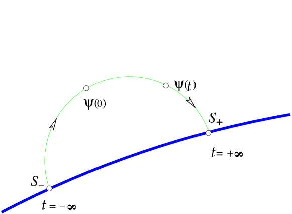
Figure 1: Convergence to stationary states

Sketch of the proof. It suffices to consider only the case $t\to\infty$. The solution admits the d’Alembert representations for $x>0$ and $x<0$, which imply the ‘reduced equation’ for $y(t):=\psi(0,t)$:

$$2\dot{y}(t)=F(y(t))+2\dot{w}_{\rm in}(t),\qquad t>0.$$ (2.18)

Here $w_{\rm in}(t)$ is the sum of incoming waves, for which $\displaystyle\int_{0}^{\infty}|\dot{w}_{\rm in}(t)|^{2}dt<\infty$. This equation provides the ‘integral of dissipation’

$$2\int_{0}^{t}|\dot{y}(s)|^{2}ds+U(y(t))=U(y(0))+2\int_{0}^{t}\dot{w}_{\rm in}(t)\cdot\dot{y}(s)\,ds,\qquad t>0,$$ (2.19)

which implies that $\displaystyle\int_{0}^{\infty}|\dot{y}(t)|^{2}dt<\infty$ according to (2.10). Hence, (2.11) implies that

$$y(t)\to Z,\qquad\dot{y}(t)\to 0,\qquad t\to\infty.$$ (2.20)

This convergence implies (2.15), since $\psi(x,t)\sim y(t-|x|)$ for large $t$ and bounded $|x|$.   

Note that the attractions (2.15) and (2.17) in the global norm of ${\cal E}$ is impossible due to outgoing d’Alembert’s waves $y(t-|x|)$, representing a solution for large $t$, which carry energy to infinity. In particular, the energy of the limiting stationary state may be smaller that the conserved energy of the solution, since the energy of the outgoing waves is irretrievably lost at infinity. Indeed, the energy is the Hamilton functional (2.9), where the integral vanishes for the limit state, and only the energy of the oscillator $U(\psi(0))$ persists. Therefore, the energy of the limit is usually smaller than the energy of the solution. This limit jump is similar to the well-known property of the weak convergence in the Hilbert space.

The discreteness of the set $Z$ is essential: asymptotics (2.17) can break down if $F(z)=0$ on $[z_{-},z_{+}]$, where $z_{-}<z_{+}$. For example, (2.17) breaks down for the solution $\psi(x,t)=\sin[\log(|x-t|+2)]$ in the case $z_{\pm}=\pm 1$.

Further, asymptotics (2.17) in the local seminorms can be extended to the asymptotics in the global norms (2.6), taking into account the outgoing d’Alembert’s waves. Namely, in [48] we have proved the following result. Let us denote by ${\cal E}_{*}$ the space of $(\phi_{0},\pi_{0})\in{\cal E}$ for which there exist the finite limits and the integral (2.2), and by ${\cal E}_{*}^{\pm}$ the subspace of ${\cal E}_{*}$ defined by the identity

$$C_{+}+C_{-}\pm\int_{-\infty}^{\infty}\pi_{0}(y)dy=0$$ (2.21)

in the notations (2.2).

Theorem 2.3.

Let conditions of Theorem 2.2 i) and ii) hold. Then for any initial state $(\phi_{0},\pi_{0})\in{\cal E}_{*}$

$$(\psi(\cdot,t),\dot{\psi}(\cdot,t))=S_{\pm}+W(t)\Phi_{\pm}+r_{\pm}(t),$$ (2.22)

where $S_{\pm}\in{\cal S}$, by $W(t)$ we denote the dynamical group of the free wave equation (2.1), $\Phi_{\pm}\in{\cal E}_{*}^{\pm}$ are some ‘scattering states’ of finite energy, and the remainder $r_{\pm}(t)$ converges to zero in the global energy norm:

$$\|r_{\pm}(t)\|_{{\cal E}}\xrightarrow[t\to\pm\infty]{}0.$$ (2.23)

The term $W(t)\Phi_{\pm}$ represents the outgoing d’Alembert’s waves, and the condition (2.21) provides that the $W(t)\Phi_{\pm}\to 0$ as $t\to\pm\infty$, according to (2.3) and (2.4). Thus, Theorem 2.3 proves the ”Grand Conjecture” [57, p.460] for equation (2.5).

Finally, the asymptotic completeness of this nonlinear scattering was established in [49, 50]. Let us fix a stationary state $S_{+}=(z_{+},0)\in{\cal S}$, and denote by ${\cal E}_{*}(S_{+})$ the set of initial states $(\psi_{0},\pi_{0})\in{\cal E}_{*}$ providing the asymptotics (2.22) with limit state $S_{+}$ as $t\to\infty$. Let $F^{\prime}(z_{+})$ denote the corresponding Jacobian matrix and $\sigma(F^{\prime}(z_{+}))$ denote its spectrum.

Theorem 2.4.

Let conditions of Theorem 2.3 hold. Then the mapping $(\psi_{0},\pi_{0})\mapsto\Phi_{+}$ is the epimorphism ${\cal E}_{*}(S_{+})\to{\cal E}_{*}^{+}$ if ${\rm Re{\hskip 1.42262pt}{\hskip 1.42262pt}}\lambda\neq 0$ for $\lambda\in\sigma(F^{\prime}(z_{+}))$.

Similar theorem holds obviously for the map $(\psi_{0},\pi_{0})\mapsto\Phi_{-}$.

2.2 Generalizations

I. In [39, 40, 48], Theorems 2.2 and 2.3 were established also for more general equation than (2.5):

$$(1+m\delta(x))\ddot{\psi}(x,t)=\psi^{\prime\prime}(x,t)+\delta(x)F(\psi(0,t)),\qquad x\in\mathbb{R},$$ (2.24)

where $m>0$ is the mass of the particle attached to the string at the point $x=0$. In this case the Hamiltonian (2.9) includes the additional term $mv^{2}/2$, where $v=\dot{\psi}(0,t)$. Moreover, the reduced equation (2.18) now becomes the Newton equation with the friction:

$$m\ddot{y}(t)=F(y(t))-2\dot{y}(t)+2\dot{w}_{\rm in}(t),\qquad t>0.$$ (2.25)

II. In [41], we have proved the convergence (2.15) and (2.17) to a global attractor for the string with $N$ oscillators:

$$\ddot{\psi}(x,t)=\psi^{\prime\prime}(x,t)+\sum_{1}^{N}\delta(x-x_{k})F_{k}(\psi(x_{k},t)).$$ (2.26)

The equation is reduced to a system of $N$ equations with delay, but its study requires novel arguments, since the oscillators are connected at different moments of time.
III. In [42], the result was extended to equations of the type

$$\ddot{\psi}(x,t)=\psi^{\prime\prime}(x,t)+\chi(x)F(\psi(x,t)),$$ (2.27)

where $\chi\in C_{0}^{\infty}(\mathbb{R})$, $\chi(x)\geq 0$, and $\chi(x)\not\equiv 0$ while $F$ has structure (2.7) with potential $U$ satisfying (2.10). This guarantees the existence of global solutions of finite energy and conservation of the Hamilton functional

$${\cal H}(\psi,\pi)=\frac{1}{2}\int[|\pi(x)|^{2}+|\psi^{\prime}(x)|^{2}+\chi(x)U(\psi(x))]\,dx.$$ (2.28)

Sketch of the proof. Again it suffices to consider only the case $t\to\infty$. For the proof of (2.15) and (2.17) in this case we develop our approach [41] based on the finiteness of energy radiated from an interval $[-a,a]\supset{\rm supp{\hskip 1.42262pt}}\chi$, which implies the finiteness of ‘integral of dissipation’ [42, (6.3)]:

$$\int[|\dot{\psi}(-a,t)|^{2}+|\psi^{\prime}(-a,t)|^{2}+|\dot{\psi}(a,t)|^{2}+|\psi^{\prime}(a,t)|^{2}]dt<\infty.$$ (2.29)

This means, roughly speaking, that

$$\psi(\pm a,t)\sim C_{\pm},\qquad\psi^{\prime}(\pm a,t)\sim 0,\qquad t\to\infty.$$ (2.30)

It remains to justify the correctness of the boundary value problem for nonlinear differential equation (2.27) in the band $-a\leq x\leq a$, $t>0$, with the Cauchy boundary conditions (2.30) on the sides $x=\pm a$. This correctness should imply the convergence of type

$$\psi(x,t)\sim S(x),\qquad t\to\infty.$$ (2.31)

The proof employs the symmetry of the wave equation with respect to permutations of variables $x$ and $t$ with simultaneous change of sign of the potential $U$. In this boundary-value problem the variable $x$ plays the role of time, and condition (2.10) makes the potential unbounded from below! Hence, this dynamics with $x$ as ‘time variable’ is not globally correct on the interval $|x|\leq a$: for example, in the ordinary equation $\psi^{\prime\prime}(x)-U^{\prime}(\psi)=0$ with $U=\psi^{4}$, a solution can run away at a point $x\in(-a,a)$. However, in our setting the local correctness is sufficient in view of the a priori estimates, which follow from the conservation of energy (2.28) due to the conditions (2.10) and $\chi(x)\geq 0$, $\chi(x)\not\equiv 0$.   
A detailed presentation of the results [39]–[42] is available in the survey [43].

2.3 Wave-particle system

In [44] we have proved the first result on the global attraction (1.5) for the 3-dimensional real scalar wave field coupled to a relativistic particle. The 3D scalar field satisfies the wave equation

$$\ddot{\psi}(x,t)=\Delta\psi(x,t)-\rho(x-q(t)),\qquad x\in\mathbb{R}^{3},$$ (2.32)

where $\rho\in C^{\infty}_{0}(\mathbb{R}^{3})$ is a fixed function, representing the charge density of the particle, and $q(t)\in\mathbb{R}^{3}$ is the particle position. The particle motion obeys the Hamilton equations with the relativistic kinetic energy $\sqrt{1+p^{2}}$:

$$\dot{q}(t)=\frac{p(t)}{\sqrt{1+p^{2}(t)}},\qquad\dot{p}(t)=-\nabla V(q(t))-\int\nabla\psi(x,t)\rho(x-q(t))\,dx.$$ (2.33)

Here, $-\nabla V(q)$ is the external force produced by some real potential $V(q)$, and the integral is the self-force. This means that the wave function $\psi$, generated by the particle, plays the role of a potential acting on the particle, along with the external potential $V(q)$.

Definition 2.5.

${\cal E}:=H^{1}(\mathbb{R}^{3})\oplus L^{2}(\mathbb{R}^{3})\oplus\mathbb{R}^{3}\oplus\mathbb{R}^{3}$ is the Hilbert phase space of tetrads $(\psi,\pi,q,p)$ with finite norm

$$\|(\psi,\pi,q,p)\|_{{\cal E}}=\|\nabla\psi\|+\|\psi\|+\|\pi\|+|q|+|p|,$$ (2.34)

where $\|\cdot\|$ is the norm in $L^{2}:=L^{2}(\mathbb{R}^{3})$.

System (2.32)–(2.33) is equivalent to the Hamilton system

$$\left\{\begin{array}[]{rclrcl}\dot{\psi}(t)&=&D_{\pi}{\cal H}(\psi(t),\pi(t),q(t),p(t)),&\qquad\dot{\pi}(t)&=&-D_{\psi}{\cal H}(\psi(t),\pi(t),q(t),p(t))\\ \\ \dot{q}(t)&=&D_{p}{\cal H}(\psi(t),\pi(t),q(t),p(t)),&\qquad\dot{p}(t)&=&-D_{q}{\cal H}(\psi(t),\pi(t),q(t),p(t))\end{array}\right|$$ (2.35)

with the conserved Hamilton functional

$${\cal H}(\psi,\pi,q,p)\!=\!\displaystyle\frac{1}{2}\!\int[|\pi(x)|^{2}\!+\!|\nabla\psi(x)|^{2}]\,dx\!+\!\int\psi(x)\rho(x\!-\!q)\,dx\!+\!\sqrt{1\!+\!p^{2}}\!+\!V(q),\quad(\psi,\pi,q,p)\in{\cal E}.$$ (2.36)

This functional is defined and is Gâteaux-differentiable on the Hilbert phase space ${\cal E}$.

We assume that the potential $V(q)\in C^{2}(\mathbb{R}^{3})$ is confining:

$$V(q)\xrightarrow[|q|\to\infty]{}\infty.$$ (2.37)

In this case it is easy to prove that the finite energy solution $Y(t)=(\psi(t),\pi(t),q(t),p(t))\in C(\mathbb{R},{\cal E})$ exists and is unique for any initial state $Y(0)\in{\cal E}$.

In the case of a point particle $\rho(x)=\delta(x)$ the system (2.32)–(2.33) is undetermined. Indeed, in this setting any solution to the wave equation (2.32) is singular at $x=q(t)$, and respectively, the integral on the right of (2.33) does not exist.

We denote $Z=\{z\in\mathbb{R}^{3}:$ $\nabla V(z)=0\}$. It is easily checked that the stationary states of the system (2.32)–(2.33) are of the form

$$S_{z}=(\psi_{z},0,z,0),$$ (2.38)

where $z\in Z$, while $\Delta\psi_{z}(x)=\rho(x-z)$; i.e.,

$$\psi_{z}(x):=-\displaystyle\frac{1}{4\pi}\int\frac{\rho(y-z)\,dy}{|x-y|}$$

is the Coulomb potential. Respectively, the set of all stationary states of this system is given by

$${\cal S}:=\{S_{z}:z\in Z\}.$$ (2.39)

If the set $Z\subset\mathbb{R}^{N}$ is discrete, then ${\cal S}$ is also discrete in ${\cal E}$. Finally, we assume that the ‘form factor’ $\rho$ satisfies the Wiener condition

$$\hat{\rho}(k):=\int e^{ikx}\rho(x)\,dx\neq 0,\qquad k\in\mathbb{R}^{3}.$$ (2.40)

It means the strong coupling of the scalar field $\psi(x)$ with the particle.

Let us denote $B_{R}=\{x\in\mathbb{R}^{3}:|x|<R\}$ for $R>0$ and let $\|\cdot\|_{R}$ stand for the norm in $L^{2}(B_{R})$. We define the local energy seminorms

$$\|(\psi,\pi,q,p)\|_{{\cal E}_{R}}=\|\nabla\psi\|_{R}+\|\psi\|_{R}+\|\pi\|+|q|+|p|$$ (2.41)

on the Hilbert phase space ${\cal E}$. The main result of [44] is the following.

Theorem 2.6.

i) Let conditions (2.37), (2.40) hold, and let $Y(t)=(\psi(t),\pi(t),q(t),p(t))$ be a finite energy solution to the system (2.32)–(2.33). Then

$$Y(t)\xrightarrow[t\to\pm\infty]{}{\cal S},$$ (2.42)

where the convergence holds in the metric (2.14) with seminorm (2.41).
ii) Let moreover, the set $Z$ be discrete in $\mathbb{R}^{N}$. Then

$$Y(t)\xrightarrow[t\to\pm\infty]{}S_{\pm}\in{\cal S},$$ (2.43)

where the convergence holds in the same metric.

Sketch of the proof. The key point in the proof is the relaxation of acceleration

$$\ddot{q}(t)\xrightarrow[t\to\pm\infty]{}0,$$ (2.44)

which follows from the Wiener condition (2.40). Then the asymptotics (2.42) and (2.43) immediately follow from this relaxation and from (2.37) by the Liénard-Wiechert representations for the potentials.

Let us explain how to deduce (2.44) as $t\to\infty$ in the case of spherically symmetric form factor $\rho(x)=\rho_{1}(|x|)$. The energy conservation and condition (2.37) imply the a priori estimate $|p(t)|\leq{\rm const}$, and hence

$$|\dot{q}(t)|\leq\overline{v}<1$$ (2.45)

by the first equation of (2.33). The radiated energy during the time $0<t<\infty$ is finite by condition (2.37):

$$E_{\rm rad}=\lim_{R\to\infty}\int_{0}^{\infty}\Big{[}\int_{|x|=R}S(x,t)\cdot\frac{x}{|x|}d^{2}x\Big{]}dt<\infty,$$ (2.46)

where $S(x,t)=-\pi(x,t)\nabla\psi(x,t)$ is the density of energy flux. Let us denote

$$R_{\omega}(t):=\int\rho(y-q(t+\omega\cdot y))\frac{\omega\cdot\ddot{q}(t+\omega\cdot y)}{[1-\omega\cdot\dot{q}(t+\omega\cdot y)]^{2}}dy,\qquad\omega\in\mathbb{R}^{3},\,|\omega|=1.$$ (2.47)

It turns out that the finiteness of energy radiation (2.46) also implies the finiteness of the integral

$$I_{\rm rad}=\int_{0}^{\infty}\Big{[}\int_{|\omega|=1}|R_{\omega}(t)|^{2}{\hskip 1.42262pt}d^{2}\omega\Big{]}dt<\infty,$$ (2.48)

which represents the contribution of the Liénard–Wiechert retarded potentials. Furthermore, the function $R(\omega,t)$ is globally Lipschitz in view of (2.45). Hence,

$$R_{\omega}(t)\xrightarrow[t\to\infty]{}0,\quad|\omega|=1.$$ (2.49)

To deduce (2.44), it is necessary to rewrite (2.47) as a convolution. We denote $r(s):=\omega\cdot q(s)$ and observe that the map $s\mapsto\theta:=s-r(s)$ is a diffeomorphism from $\mathbb{R}$ to $\mathbb{R}$, inasmuch as $|\dot{r}(s)|\leq\overline{v}<1$ by (2.45). Then the desired convolution representation reads

$$R_{\omega}(t)=[\rho_{a}*g_{\omega}](t):=\int\rho_{a}(t-\theta)g_{\omega}(\theta){\hskip 1.42262pt}d\theta,\qquad\rho_{a}(q_{1}):=\int dq_{2}dq_{3}\rho(q_{1},q_{2},q_{3}),$$ (2.50)

where

$$g_{\omega}(\theta):=[1-\dot{r}(s(\theta))]^{-3}\ddot{r}(s(\theta)),\qquad\theta\in\mathbb{R}.$$ (2.51)

It remains to note that $[\rho_{a}*g_{\omega}](t)\to 0$ by (2.49), while the Fourier transform $\tilde{\rho}_{a}(k)\neq 0$ for $k\in\mathbb{R}$ by (2.40). Now (2.44) follows from the Wiener Tauberian theorem.   

In [44] we have also proved the asymptotic stability of stationary states $S_{z}$ with positive Hessian $d^{2}V(z)\nobreak>0$.

Remark 2.7.

i) The proof of relaxation (2.44) does not depend on the condition (2.37). In particular,  (2.44) holds for $V=0$.
ii) The Wiener condition (2.40) is sufficient for the relaxation (2.44) for solutions to the system  (2.32)–(2.33). However, it is not necessary for some specific classes of potentials and solutions in the case of small $\|\rho\|$, see Section 4.3.

2.4 Maxwell-Lorentz equations: radiation damping

In [45] the attractions (2.42), (2.43) were extended to the Maxwell equations in $\mathbb{R}^{3}$ coupled to a relativistic particle:

$$\!\!\left\{\!\!\begin{array}[]{l}\dot{E}(x,t)\!=\!{\rm rot~{}}B(x,t)-\dot{q}\rho(x\!-\!q),\ \dot{B}(x,t)\!=\!-{\rm rot~{}}E(x,t),\ {\rm div~{}}E(x,t)\!=\!\rho(x\!-\!q),\ {\rm div~{}}B(x,t)\!=\!0\\ \\ \dot{q}(t)\!=\!\displaystyle\frac{p(t)}{\sqrt{1\!+\!p^{2}}(t)},\qquad\,\,\dot{p}(t)\!=\!\displaystyle\int[E(x,t)\!+\!E^{\rm ext}(x)\!+\!\dot{q}(t)\times(B(x,t)\!+\!B^{\rm ext}(x))]\rho(x\!-\!q(t))\,dx\end{array}\!\!\right|$$ (2.52)

where $\rho(x-q)$ is the charge density of a particle, $\dot{q}\rho(x-q)$ is the corresponding current density, and $E^{\rm ext}(x)=-\nabla\phi^{\rm ext}(x)$, $B^{\rm ext}(x)=-{\rm rot~{}}A^{\rm ext}(x)$ are external Maxwell fields. Similarly to (2.37), we assume that

$$V(q):=\int\phi^{\rm ext}(x)\rho(x-q)\,dx\xrightarrow[|q|\to\infty]{}\infty.$$ (2.53)

This system describes the classical electrodynamics of an ‘extended electron’ introduced by Abraham [127, 128]. In the case of a point electron, when $\rho(x)=\delta(x)$, such a system is undetermined. Indeed, in this setting any solutions $E(x,t)$ and $B(x,t)$ to the Maxwell equations (the first line of (2.52)) are singular at $x=q(t)$, and respectively, the integral on the right of the last equation in (2.52) does not exist.

The system (2.52) is time reversible in the following sense: if $E(x,t)$, $B(x,t)$, $q(t)$, $p(t)$ is its solution, then $E(x,-t)$, $-B(x,-t)$, $q(-t)$, $-p(-t)$ is also the solution to (2.52) with external fields $E^{\rm ext}(x)$, $-B^{\rm ext}(x)$. This system can be represented in the Hamilton form if the fields are expressed via the potentials $E(x,t)=-\nabla\phi(x,t)-\dot{A}(x,t)$, $B(x,t)=-{\rm rot~{}}A(x,t)$. The corresponding Hamilton functional is as follows

$${\cal H}=\frac{1}{2}[\langle E,E\rangle+\langle B,B\rangle]+V(q)+\sqrt{1+p^{2}}=\frac{1}{2}\int[E^{2}(x)+B^{2}(x)]\,dx+V(q)+\sqrt{1+p^{2}}.$$ (2.54)

This Hamiltonian is conserved, since

$$\dot{\cal H}(t) = \langle E(x,t),\dot{E}(x,t)\rangle+\langle B(x,t),\dot{B}(x,t)\rangle+\nabla V(q)\cdot\dot{q}(t)+\dot{q}(t)\cdot\dot{p}(t)$$

$$= \langle E(x,t),{\rm rot~{}}B(x,t)-\dot{q}(t)\rho(x-q(t))\rangle-\langle B(x,t),{\rm rot~{}}E(x,t)\rangle-\langle E^{\rm ext}(x),\rho(x-q(t))\rangle\cdot\dot{q}(t)$$

$$+\dot{q}(t)\cdot\langle E(x,t)+E^{\rm ext}(x)+\dot{q}(t)\times(B(x,t)+B^{\rm ext}(x)),\rho(x-q(t))\rangle$$

$$= \langle E(x,t),{\rm rot~{}}B(x,t)\rangle-\langle B(x,t),{\rm rot~{}}E(x,t)\rangle=-\lim_{R\to\infty}\int_{|x|<R}{\rm div~{}}[E(x,t)\times B(x,t)]dx$$

$$= -\lim_{R\to\infty}\int_{|x|=R}[E(x,t)\times B(x,t)]\cdot\frac{x}{|x|}\,dS(x)=0.$$ (2.55)

This energy conservation gives a priori estimates of solutions, which play an important role in the proof of the attractions of type (2.42), (2.43) in [45]. The key role in these proofs again plays the relaxation of the acceleration (2.44) which follows by a suitable development of our methods [44]: an expression of type (2.48) for the radiated energy via the Liénard-Wiechert retarded potentials, the convolution representation of type (2.50), and the application of the Wiener Tauberian theorem.

In Classical Electrodynamics the relaxation (2.44) is known as the radiation damping. It is traditionally justified by the Larmor and Liénard formulas [46, (14.22)] and [46, (14.24)] for the power of radiation of a point particle. These formulas are deduced from the Liénard-Wiechert expressions for the retarded potentials neglecting the initial field and the ”velocity field”. Moreover, the traditional approach neglects the back field-reaction though it should be the key reason for the relaxation. The main problem is that this back field-reaction is infinite for the point particles. The rigorous meaning to these calculations has been suggested first in [44, 45] for the Abraham model of the ‘extended electron’ under the Wiener condition (2.40). The survey can be found in [47].

Remark 2.8.

All the above results on the attraction of type (1.5) relate to ‘generic’ systems with the trivial symmetry group, which are characterized by the discreteness of attractors, the Wiener condition, etc.

3 Global attraction to stationary orbits

The global attraction to stationary orbits (1.6) was first proved in [100, 101, 102] for the Klein–Gordon equation coupled to the nonlinear oscillator

$$\ddot{\psi}(x,t)=\psi^{\prime\prime}(x,t)-m^{2}\psi(x,t)+\delta(x)F(\psi(0,t)),\qquad x\in\mathbb{R}.$$ (3.1)

We consider complex solutions, identifying $\psi\in{\mathbb{C}}$ with $(\psi_{1},\psi_{2})\in\mathbb{R}^{2}$, where $\psi_{1}={\rm Re{\hskip 1.42262pt}{\hskip 1.42262pt}}\psi$, $\psi_{2}={\rm Im{\hskip 1.42262pt}{\hskip 1.42262pt}}\psi$. We assume that $F\in C^{1}(\mathbb{R}^{2},\mathbb{R}^{2})$ and

$$F(\psi)=-\nabla_{\overline{\psi}}U(\psi),\qquad\psi\in{\mathbb{C}},$$ (3.2)

where $U$ is a real function, and $\nabla_{\overline{\psi}}:=\partial_{1}+i\partial_{2}$. In this case equation (3.1) is a Hamilton system of form (2.35) with the Hilbert phase space ${\cal E}:=H^{1}(\mathbb{R})\oplus L^{2}(\mathbb{R})$ and the conserved Hamilton functional

$${\cal H}(\psi,\pi)=\frac{1}{2}\int\Big{[}|\pi(x)|^{2}+|\psi^{\prime}(x)|^{2}+m^{2}|\psi(x)|^{2}\Big{]}\,dx+U(\psi(0)),\qquad(\psi,\pi)\in{\cal E}.$$ (3.3)

We assume that

$$\inf_{\psi\in{\mathbb{C}}}U(\psi)>-\infty.$$ (3.4)

In this case a finite energy solution $Y(t)=(\psi(t),\pi(t))\in C(\mathbb{R},{\cal E})$ exists and is unique for any initial state $Y(0)\in{\cal E}$. The a priori estimate

$$\sup_{t\in\mathbb{R}}[\|\pi(t)\|_{L^{2}(\mathbb{R})}+\|\psi(t)\|_{H^{1}(\mathbb{R})}]<\infty$$ (3.5)

holds due to the conservation of Hamilton functional (3.3). Note that condition (2.10) now is not necessary, since the conservation of functional (3.3) with $m>0$ provides boundedness of the solution.

Further, we assume the $U(1)$-invariance of the potential:

$$U(\psi)=u(|\psi|),\qquad\psi\in{\mathbb{C}}.$$ (3.6)

Then the differentiation (3.2) gives

$$F(\psi)=a(|\psi|)\psi,\qquad\psi\in{\mathbb{C}},$$ (3.7)

and hence,

$$F(e^{i\theta}\psi)=e^{i\theta}F(\psi),\qquad\theta\in\mathbb{R}.$$ (3.8)

By ‘stationary orbits’ (or solitons) we shall understand any solutions of the form $\psi_{\omega}(x,t)=\phi_{\omega}(x)e^{-i\omega t}$ with $\phi_{\omega}\in H^{1}({\mathbb{R}})$ and $\omega\in{\mathbb{R}}$. Each stationary orbit provides the corresponding solution to the nonlinear eigenfunction problem

$$-\omega^{2}\phi_{\omega}(x)=\phi^{\prime\prime}_{\omega}(x)-m^{2}\phi_{\omega}(x)+\delta(x)F(\phi_{\omega}(0)),\qquad x\in\mathbb{R}.$$ (3.9)

The solutions $\phi_{\omega}\in H^{1}({\mathbb{R}})$ have the form $\phi_{\omega}(x)=Ce^{-\kappa|x|}$, where $\kappa:=\sqrt{m^{2}-\omega^{2}}>0$ and $C$ satisfies the equation

$$2\kappa C=F(C).$$

Hence, the solutions exist for $\omega\in\Omega$, where $\Omega$ is a subset of the spectral gap $[-m,m]$. Let us define the corresponding solitary manifold

$${\cal S}=\{(e^{i\theta}\phi_{\omega},-i\omega e^{i\theta}\phi_{\omega})\in{\cal E}:\omega\in\Omega,~{}\theta\in[0,2\pi]\}.$$ (3.10)

Finally, we assume that equation (3.1) is strictly nonlinear:

$$U(\psi)=u(|\psi|^{2})=\Sigma_{0}^{N}u_{j}|\psi|^{2j},\quad u_{N}>0,\quad N\geq 2.$$ (3.11)

For example, the known Ginzburg–Landau potential $U(\psi)=|\psi|^{4}/4-|\psi|^{2}/2$ satisfies all conditions (3.4), (3.6) and (3.11).

Theorem 3.1.

Let conditions (3.2), (3.4), (3.6) and (3.11) hold. Then any finite energy solution $Y(t)=(\psi(t),\pi(t))$ to equation (3.1) converges to the solitary manifold in the long time limits (see Fig. 2):

$$Y(t)\xrightarrow[t\to\pm\infty]{}{\cal S},$$ (3.12)

where the convergence holds in the sense of (2.16).

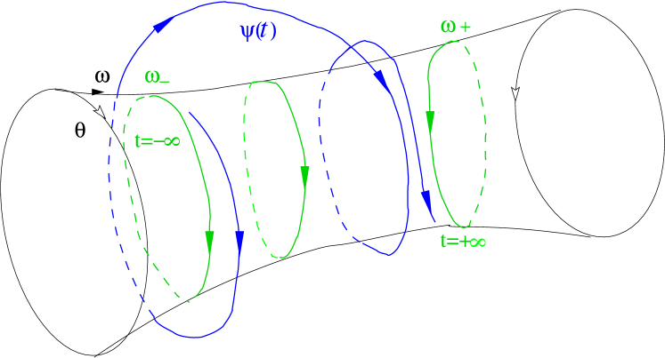
Figure 2: Convergence to stationary orbits

Generalizations: Attraction (3.12) is extended in [103] to the 1D Klein–Gordon equation with $N$ nonlinear oscillators

$$\ddot{\psi}(x,t)=\psi^{\prime\prime}(x,t)-m^{2}\psi+\sum\limits_{k=1}^{N}\delta(x-x_{k})F_{k}(\psi(x_{k},t)),~{}x\in\mathbb{R},$$ (3.13)

and in [105, 106], to the nD Klein–Gordon and Dirac equations with a ‘nonlocal interaction’

$$\ddot{\psi}(x,t) = \Delta\psi(x,t)-m^{2}\psi+\rho(x)F(\langle\psi(\cdot,t),\rho\rangle),\qquad x\in\mathbb{R}^{n},$$ (3.14)

$$i\dot{\psi}(x,t) = \big{(}-i\alpha\cdot\nabla+\beta m\big{)}\psi+\rho(x)F(\langle\psi(\cdot,t),\rho\rangle),\qquad x\in\mathbb{R}^{n}$$ (3.15)

under the Wiener condition (2.40), where $\alpha=(\alpha_{1},\dotsc,\alpha_{n})$ and $\beta=\alpha_{0}$ are the Dirac matrices.
Furthermore, attraction (3.12) is extended in [107] to discrete in space and time nonlinear Hamilton equations, which are discrete approximations of equations like (3.14). The proof relies on the new refined version of the Titchmarsh theorem for distributions on the circle, as obtained in [108].

Open questions:
I. Attraction (1.6) to the orbits with fixed frequencies $\omega_{\pm}$.
II. Attraction to stationary orbits (3.12) for nonlinear Schrödinger equations. In particular, for the 1D Schrödinger equation coupled to a nonlinear oscillator

$$i\dot{\psi}(x,t)=-\psi^{\prime\prime}(x,t)+\delta(x)F(\psi(0,t)),\qquad x\in\mathbb{R}$$ (3.16)

(see Remark 3.12).
III. Attraction to solitons (1.9) for the relativistically-invariant nonlinear Klein–Gordon equations. In particular, for the 1D equations

$$\ddot{\psi}(x,\!t)=\psi^{\prime\prime}(x,t)-m^{2}\psi(x,t)+F(\psi(x,t)).$$

Below we give a schematic proof of Theorem 3.1 in a more simple case of the zero initial data:

$$\psi(x,0)=0,\qquad\dot{\psi}(x,0)=0.$$ (3.17)

The general case of nonzero initial data is reduced to (3.17) by a trivial subtraction [100, 102]. The proof relies on a new strategy, which was first introduced in [100] and refined in [102]. The main steps of the strategy are the following:
(1) The Fourier transform in time for finite energy solutions to the nonlinear equation (3.1).
(2) Absolute continuity of the Fourier transform on the continuous spectrum of the free Klein-Gordon equation.
(3) The reduction of spectrum of omega-limit trajectories to a subset of the corresponding spectral gap.
(4) The reduction of this subset to a single point.
The steps (2) and (4) are central in the proof. The property (2) is a nonlinear analog of the Kato Theorem on the absence of embedded eigenvalues in the continuous spectrum; it implies (3). Step (4) is justified by the Titchmarsh convolution theorem. It means that the limiting behavior of any finite energy solution is single-frequency, which essentially coincides with asymptotics (1.6). An important technical role plays the application of the theory of quasi-measures and their multipliers [102, Appendix B].

The strategy (1)–(4) was also employed in [105]–[107].

3.1 Spectral representation and quasi-measures

It suffices to prove attraction (3.12) only for positive times:

$$Y(t)\xrightarrow[t\to+\infty]{}{\cal S},$$ (3.18)

We extend $\psi(x,t)$ and $f(t):=F(\psi(0,t))$ by zero for $t<0$ and denote

$$\psi_{+}(x,t):=\left\{\begin{array}[]{ll}\psi(x,t),&t>0,\\ 0,&t<0,\end{array}\right.\qquad f_{+}(t):=\left\{\begin{array}[]{ll}f(t),&t>0,\\ 0,&t<0.\end{array}\right.$$ (3.19)

By (3.1) and (3.17) these functions satisfy the following equation

$$\ddot{\psi}_{+}(x,t)=\psi_{+}^{\prime\prime}(x,t)-m^{2}\psi_{+}(x,t)+\delta(x)f_{+}(t),\qquad(x,t)\in\mathbb{R}^{2}$$ (3.20)

in the sense of distributions. We denote by $\tilde{g}(\omega)$ the Fourier transform of the tempered distribution $g(t)$ given by

$$\tilde{g}(\omega)=\int_{\mathbb{R}}e^{i\omega t}g(t)\,dt,\qquad\omega\in\mathbb{R}$$ (3.21)

for test functions $g\in C_{0}^{\infty}(\mathbb{R})$. It is important that $\psi_{+}(x,t)$ and ${}_{+}f(t)$ are bounded functions of $t\in\mathbb{R}$ with values in the Sobolev space $H^{1}(\mathbb{R})$ and ${\mathbb{C}}$, respectively, due to the a priori estimate (3.5). Now the Paley–Wiener theorem [42, p. 161] implies that their Fourier transforms admit an extension from the real axis to an analytic functions of $\omega\in{\mathbb{C}}^{+}:=\{\omega\in{\mathbb{C}}:~{}{\rm Im{\hskip 1.42262pt}{\hskip 1.42262pt}}\omega>0\}$ with values in $H^{1}(\mathbb{R})$ and ${\mathbb{C}}$, respectively:

$$\tilde{\psi}_{+}(x,\omega)=\int_{0}^{\infty}e^{i\omega t}\psi(x,t)\,dt,\qquad\tilde{f}_{+}(\omega)=\int_{0}^{\infty}e^{i\omega t}f(t)\,dt,\qquad\omega\in{\mathbb{C}}^{+}.$$ (3.22)

These functions grow not faster than $|{\rm Im{\hskip 1.42262pt}{\hskip 1.42262pt}}\omega|^{-1}$ as ${\rm Im{\hskip 1.42262pt}{\hskip 1.42262pt}}\omega\to 0+$ in view of (3.5). Hence, their boundary values at $\omega\in\mathbb{R}$ are the distributions of a low singularity: they are second-order derivatives of continuous functions as in the case $\tilde{f}_{+}(\omega)=i/(\omega-\omega_{0})$ with $\omega_{0}\in{\mathbb{R}}$, which corresponds to $f_{+}(t)=\theta(t)e^{-i\omega_{0}t}$.

Recall that the Fourier transform of functions from $L^{\infty}(\mathbb{R})$ are called quasi-measures [110]. Further we will use a special weak ‘Ascoli–Arzela’ convergence in the space $L^{\infty}(\mathbb{R})$:

Definition 3.2.

For $g,g_{n}\in L^{\infty}(\mathbb{R})$ the convergence $g_{n}\stackrel{{\scriptstyle\cal AA}}{{\mathop{\longrightarrow}}}g$ means that

$$\lim_{n\to\infty}\|g_{n}(t)-g(t)\|_{L^{\infty}(-T,T)}=0\ \ \ \forall T>0\quad\mbox{and}\quad\sup_{n}\|g_{n}\|_{L^{\infty}(\mathbb{R})}<\infty.$$ (3.23)

Definition 3.3.

i) A tempered distribution $\mu(\omega)$ is called a quasi-measure if $\mu=\tilde{g}$, where $g\in L^{\infty}(\mathbb{R})$.

ii) ${\cal Q}{\cal M}$ denotes the linear space of quasi-measures endowed with the following convergence: for a sequence $\mu_{n}=\tilde{g}_{n}\in{\cal Q}{\cal M}$ with $g_{n}\in L^{\infty}(\mathbb{R})$

$$\mu_{n}\stackrel{{\scriptstyle\cal QM}}{{\mathop{\longrightarrow}}}\mu\quad\mbox{if and only if}\quad g_{n}\stackrel{{\scriptstyle\cal AA}}{{\mathop{\longrightarrow}}}g.$$ (3.24)

The following technical lemma will play an important role in our analysis. Denote $L^{1}:=L^{1}(\mathbb{R})$.

Lemma 3.4.

i) The function $M(\omega)$ is a multiplier in ${\cal Q}{\cal M}$ if $M=\tilde{G}$, where $G\in L^{1}$.

ii) Let $\mu_{n}\stackrel{{\scriptstyle\cal QM}}{{\mathop{\longrightarrow}}}\mu$, and $G_{n}\stackrel{{\scriptstyle L^{1}}}{{\mathop{\longrightarrow}}}G$. Then, for $M_{n}:=\tilde{G}_{n}$ and $M=\tilde{G}$,

$$M_{n}\mu_{n}\stackrel{{\scriptstyle\cal QM}}{{\mathop{\longrightarrow}}}M\mu.$$ (3.25)

For the proof it suffices to verify that $G_{n}*g_{n}\stackrel{{\scriptstyle\cal AA}}{{\mathop{\longrightarrow}}}G*g$ if $g_{n}\stackrel{{\scriptstyle\cal AA}}{{\mathop{\longrightarrow}}}g$.
Further, by (3.17) equation (3.20) in the Fourier transform reads as the stationary Helmholtz equation

$$-\omega^{2}\tilde{\psi}_{+}(x,\omega)=\tilde{\psi}_{+}^{\prime\prime}(x,\omega)-m^{2}\tilde{\psi}_{+}(x,\omega)+\delta(x)\tilde{f}_{+}(\omega),\qquad x\in\mathbb{R}.$$ (3.26)

Its solution is given by

$$\tilde{\psi}_{+}(x,\omega)=-\tilde{f}_{+}(\omega)\frac{e^{ik(\omega)|x|}}{2ik(\omega)},\qquad{\rm Im{\hskip 1.42262pt}{\hskip 1.42262pt}}\omega>0.$$ (3.27)

Here $k(\omega):=\sqrt{\omega^{2}-m^{2}}$, where the branch of the root is chosen to be analytic for ${\rm Im{\hskip 1.42262pt}{\hskip 1.42262pt}}\omega>0$ and having positive imaginary part. For this branch, the right-hand side of equation (3.27) belongs to $H^{1}(\mathbb{R})$ in accordance with the properties of $\tilde{\psi}_{+}(x,\omega)$, while for the other branch the right-hand side grows exponentially as $|x|\to\infty$. Such argument for the choice of the solution is known as the ‘limiting absorption principle’ in the theory of diffraction [94]. We will write (3.27) as

$$\tilde{\psi}_{+}(x,\omega)=\tilde{\alpha}(\omega)e^{ik(\omega)|x|},\qquad{\rm Im{\hskip 1.42262pt}{\hskip 1.42262pt}}\omega>0,$$ (3.28)

where $\alpha(t):=\psi_{+}(0,t)$. A nontrivial observation is that equality (3.28) of analytic functions implies the similar identity for their restrictions to the real axis:

$$\tilde{\psi}_{+}(x,\omega+i0)=\tilde{\alpha}(\omega+i0)e^{ik(\omega+i0)|x|},\qquad\omega\in\mathbb{R},$$ (3.29)

where $\tilde{\psi}_{+}(\cdot,\omega+i0)$ and $\tilde{\alpha}(\omega+i0)$ are the corresponding quasi-measures with values in $H^{1}(\mathbb{R})$ and ${\mathbb{C}}$, respectively. The problem is that the factor $M_{x}(\omega):=e^{ik(\omega+i0)|x|}$ is not smooth in $\omega$ at the points $\omega=\pm m$, and so identity (3.29) requires a justification.

Lemma 3.5.

([102, Proposition 3.1]) For each $x\in\mathbb{R}$,

$$\tilde{\alpha}(\omega+i\varepsilon)\stackrel{{\scriptstyle\cal QM}}{{\mathop{\longrightarrow}}}\tilde{\alpha}(\omega+i0)\quad\mbox{\rm and}\quad G_{x}(\omega+i\varepsilon)\stackrel{{\scriptstyle L^{1}}}{{\mathop{\longrightarrow}}}G_{x}(\omega+i0)\qquad\mbox{\rm as}\quad\varepsilon\to 0+,$$ (3.30)

where $\tilde{G}_{x}(\omega+i\varepsilon)=M_{x}(\omega+i\varepsilon)$ and $\tilde{G}_{x}(\omega+i0)=M_{x}(\omega+i0)$.

Now (3.29) follows from Lemma 3.4.

Finally, the inversion of the Fourier transform can be written as

$$\psi_{+}(x,t)=\frac{1}{2\pi}\int_{\mathbb{R}}e^{-i\omega t}\tilde{\psi}_{+}(x,\omega+i0)\,d\omega=\frac{1}{2\pi}\int_{\mathbb{R}}e^{-i\omega t}\tilde{\alpha}(\omega+i0)e^{ik(\omega+i0)|x|}d\omega,\qquad t>0,\quad x\in\mathbb{R}.$$ (3.31)

3.2 A nonlinear analogue of the Kato theorem

It turns out that properties of the quasi-measure $\tilde{\alpha}(\omega+i0)$ for $|\omega|<m$ and for $|\omega|>m$ differ greatly. This is due to the fact that the set $\{i\omega:|\omega|\geq m\}$ coincides, up to the factor $i$, with the continuous spectrum of the generator

$$A=\left(\begin{array}[]{cc}0&1\\ \frac{d^{2}}{dx^{2}}-m^{2}&0\end{array}\right)$$ (3.32)

of the linear part of (3.1). The following proposition plays the key role in our proofs. It is a non-linear analogue of the Kato theorem on the absence of embedded eigenvalues in the continuous spectrum. Let us denote $\Sigma:=\{\omega\in\mathbb{R}:|\omega|>m\}$, and we will write below $\tilde{\alpha}(\omega)$ and $k(\omega)$ instead of $\tilde{\alpha}(\omega+i0)$ and $k(\omega+i0)$ for $\omega\in{\mathbb{R}}$.

Proposition 3.6.

([102, Proposition 3.2]) Let conditions (3.2), (3.4) and (3.6) hold and let $\psi(t)$ be a finite energy solution of equation (3.1). Then the distribution $\tilde{\alpha}(\omega):=\tilde{\alpha}(\omega+i0)$ is absolutely continuous on $\Sigma$, and $\tilde{\alpha}\in L^{1}(\Sigma)$. Moreover,

$$\int_{\Sigma}|\tilde{\alpha}(\omega)|^{2}{\hskip 1.42262pt}|\omega{\hskip 1.42262pt}k(\omega)|{\hskip 1.42262pt}d\omega<\infty.$$ (3.33)

The proof [102] relies on the integral representation (3.31), the a priori estimate (3.5), and uses some ideas of the Paley–Wiener theory. The main idea is that the functions $e^{ik(\omega+i0)|x|}$ in (3.31) do not belong to $H^{1}({\mathbb{R}})$ for $\omega\in\Sigma$.

3.3 Dispersive and bound components

Proposition 3.6 suggests the splitting of the solution (3.31) into the ‘dispersion’ and ‘bound’ components

$$\psi_{+}(x,t) = \frac{1}{2\pi}\int_{\Sigma}(1-\zeta(\omega))e^{-i\omega t}\tilde{\alpha}(\omega)e^{ik(\omega)|x|}d\omega+\frac{1}{2\pi}\langle\tilde{\alpha}(\omega),\zeta(\omega)e^{-i\omega t}e^{ik(\omega)|x|}\rangle$$ (3.34)

$$= \psi_{d}(x,t)+\psi_{b}(x,t),\qquad t>0,\qquad x\in\mathbb{R},$$

where

$$\zeta(\omega)\in C_{0}^{\infty}(\mathbb{R}),\qquad\zeta(\omega)=1\quad\mbox{\rm for}\quad\omega\in[-m-1,m+1],$$ (3.35)

and $\langle\,\cdot{,}\,\cdot\rangle$ is the duality between quasi-measures and the corresponding test functions (in particular, Fourier transforms of functions from $L^{1}(\mathbb{R})$). Note that $\psi_{d}(x,t)$ is a dispersion wave, because

$$\psi_{d}(x,t):=\frac{1}{2\pi}\int_{\Sigma}(1-\zeta(\omega))e^{-i\omega t}\tilde{\alpha}(\omega)e^{ik(\omega)|x|}d\omega\xrightarrow[t\to\infty]{}0$$ (3.36)

by (3.33) and the Lebesgue–Riemann theorem. The meaning of this convergence is specified in the following simple lemma.

Lemma 3.7.

([102, Lemma 3.3]) $\psi_{d}(x,t)$ is a bounded continuous function of $t\in\mathbb{R}$ with values in $H^{1}(\mathbb{R})$, and

$$(\psi_{d}(\cdot,t),\dot{\psi}_{d}(\cdot,t))\to 0$$ (3.37)

in the seminorms (2.13).

Hence, it remains to prove the attraction (3.18) for $Y_{b}(t):=(\psi_{b}(\cdot,t),\dot{\psi}_{b}(\cdot,t))$ instead of $Y(t)$:

$$Y_{b}(t)\xrightarrow[t\to+\infty]{}{\cal S}.$$ (3.38)

3.4 Compactness and omega-limit trajectories

To prove (3.38) we note, first, that the bound component $\psi_{b}(x,t)$ is a smooth function, and

$$\partial_{x}^{j}\partial_{t}^{l}\psi_{b}(x,t)=\frac{1}{2\pi}\langle\tilde{\alpha}(\omega),\zeta(\omega)(ik(\omega)\operatorname{sgn}{\hskip 1.42262pt}x)^{j}(-i\omega)^{l}e^{-i\omega t}e^{ik(\omega)|x|}\rangle,\qquad t>0,\quad x\in\mathbb{R},$$ (3.39)

which implies the boundedness of each derivative:

Lemma 3.8.

([102, Proposition 4.1]) For any $j,l=0,1,2,\dotsc$ and $R>0$

$$\sup_{0<|x|\leq R}\,\,\sup_{t\in\mathbb{R}}|\partial_{x}^{j}\partial_{t}^{l}\psi_{b}(x,t)|<\infty.$$ (3.40)

Proof. It suffices to verify that $\zeta(\omega)k^{j}(\omega)\omega^{l}e^{-i\omega t}e^{ik(\omega)|x|}=\tilde{g}_{x}(\omega)$, where $g_{x}(\cdot)$ belongs to a bounded subset of $L^{1}(\mathbb{R})$ for $0<|x|\leq R$. Then (3.40) follows from (3.39) by the Parseval identity, inasmuch as $\alpha(t):=\psi(0,t)$ is a bounded function.   

Hence, by the Ascoli–Arzela theorem, for any sequence $s_{j}\to\infty$ there exists a subsequence $s_{j^{\prime}}\to\infty$, for which

$$\partial_{x}^{j}\partial_{t}^{l}\psi_{b}(x,s_{j^{\prime}}+t)\to\partial_{x}^{j}\partial_{t}^{l}\beta(x,t),\qquad(x,t)\in\mathbb{R}^{2},$$ (3.41)

the convergence being uniform on compact sets. We will call any such function $\beta(x,t)$ an omega-limit trajectory of the solution $\psi(x,t)$. It follows from bounds (3.40) that

$$\sup_{(x,t)\in\mathbb{R}^{2}}|\partial_{x}^{j}\partial_{t}^{l}\beta(x,t)|<\infty.$$ (3.42)

Lemma 3.9.

Attraction (3.38) is equivalent to the fact that any omega-limit trajectory is a stationary orbit:

$$\beta(x,t)=\phi_{\omega_{+}}(x)e^{-i\omega_{+}t},\qquad\omega_{+}\in\mathbb{R}.$$ (3.43)

This lemma follows from the uniform convergence (3.41) on each compact set and the definition of the metric (2.14).

3.5 Spectral representation of omega-limit trajectories

Let us note that $\psi_{b}(x,t)$ is a bounded function of $t\in\mathbb{R}$ with values in $H^{1}(\mathbb{R})$ due to the similar boundedness of $\psi_{+}(x,t)$ and $\psi_{d}(x,t)$. Therefore, $\psi_{b}(x,\cdot)$ is a bounded function of $t\in\mathbb{R}^{2}$ for each $x\in\mathbb{R}$, and convergence (3.41) with $j=l=0$ implies the convergence of the corresponding Fourier transforms in time in the sense of tempered distributions. Moreover, this convergence holds in the sense of Ascoli–Arzela quasi-measures (3.24)

$$\tilde{\psi}_{b}(x,\omega)e^{-i\omega s_{j^{\prime}}}\stackrel{{\scriptstyle\cal QM}}{{\mathop{\longrightarrow}}}\tilde{\beta}(x,\omega),\qquad\forall x\in\mathbb{R}.$$ (3.44)

Hence, representation (3.39) implies that

$$\zeta(\omega)\tilde{\alpha}(\omega)e^{ik(\omega)|x|}e^{-i\omega s_{j^{\prime}}}\stackrel{{\scriptstyle\cal QM}}{{\mathop{\longrightarrow}}}\tilde{\beta}(x,\omega),\qquad\forall x\in\mathbb{R}.$$ (3.45)

Further, $e^{-ik(\omega)|x|}$ is a multiplier in the space of Ascoli–Arzela quasi-measures according [102, Lemma B.3]). Now (3.45) gives that

$$\zeta(\omega)\tilde{\alpha}(\omega)e^{-i\omega s_{j^{\prime}}}\stackrel{{\scriptstyle\cal QM}}{{\mathop{\longrightarrow}}}\tilde{\gamma}(\omega):=\tilde{\beta}(x,\omega)e^{-ik(\omega)|x|},\qquad\forall x\in\mathbb{R}.$$ (3.46)

Hence, (3.39) with $j=l=0$ and $t+s_{j^{\prime}}$ instead of $t$, gives in the limit $j^{\prime}\to\infty$ the integral representation

$$\beta(x,t)=\frac{1}{2\pi}\langle\tilde{\gamma}(\omega)e^{ik(\omega)|x|},e^{-i\omega t}\rangle,\qquad(x,t)\in\mathbb{R}^{2},$$ (3.47)

since $e^{ik(\omega)|x|}$ is a multiplier. Note that

$$\beta(0,t)=\gamma(t).$$ (3.48)

Moreover,

$${\rm supp{\hskip 1.42262pt}}\tilde{\gamma}\subset[-m,m]$$ (3.49)

by (3.46) and Proposition 3.6 due to the Riemann–Lebesgue theorem.

3.6 Equation for omega-limit trajectories and spectral inclusion

Note that $\psi_{+}(x,t)$ is a solution of (3.1) only for $t>0$ because of (3.19) and (3.20). However, the following simple but important lemma holds.

Lemma 3.10.

Any omega-limit trajectory satisfies the same equation (3.1):

$$\ddot{\beta}(x,t)=\beta^{\prime\prime}(x,t)-m^{2}\beta(x,t)+\delta(x)F(\beta(0,t)),\qquad(x,t)\in\mathbb{R}^{2}.$$ (3.50)

The lemma follows by substitution $\psi_{+}(x,s_{j^{\prime}}+t)=\psi_{d}(x,s_{j^{\prime}}+t)+\psi_{b}(x,s_{j^{\prime}}+t)$ into equation (3.20) and subsequent limit $s_{j^{\prime}}\to\infty$ taking into account (3.37) and (3.41).

The following proposition implies (3.38) by Lemma 3.9.

Proposition 3.11.

Under the hypotheses of Theorem 3.1 any omega-limit trajectory is a stationary orbit of the form (3.43).

First, (3.50) in the Fourier transform becomes the stationary equation

$$-\omega^{2}\tilde{\beta}(x,\omega)=\tilde{\beta}^{\prime\prime}(x,\omega)-m^{2}\tilde{\beta}(x,\omega)+\delta(x)\tilde{f}(\omega),\qquad(x,\omega)\in\mathbb{R}^{2},$$ (3.51)

where $f(t):=F(\beta(0,t))=F(\gamma(t))$ by (3.48). Further, (3.7) gives that

$$f(t)=a(|\gamma(t)|)\gamma(t)=A(t)\gamma(t),\qquad A(t)=a(|\gamma(t)|),\qquad t\in\mathbb{R}.$$ (3.52)

Hence, in the Fourier transform we obtain the convolution $\tilde{f}=\tilde{A}*\tilde{\gamma}$, which exists by (3.49). Respectively, (3.51) reads

$$-\omega^{2}\tilde{\beta}(x,\omega)=\tilde{\beta}^{\prime\prime}(x,\omega)-m^{2}\tilde{\beta}(x,\omega)+\delta(x)[\tilde{A}*\tilde{\gamma}](\omega),\qquad(x,\omega)\in\mathbb{R}^{2}.$$ (3.53)

This identity implies the key spectral inclusion

$${\rm supp{\hskip 1.42262pt}}\tilde{A}*\tilde{\gamma}\subset{\rm supp{\hskip 1.42262pt}}\tilde{\gamma},$$ (3.54)

since ${\rm supp{\hskip 1.42262pt}}\tilde{\beta}(x,\cdot)\subset{\rm supp{\hskip 1.42262pt}}\tilde{\gamma}$ and ${\rm supp{\hskip 1.42262pt}}\tilde{\beta}^{\prime\prime}(x,\cdot)\subset{\rm supp{\hskip 1.42262pt}}\tilde{\gamma}$ by (3.47). Using this inclusion, we will deduce below Proposition 3.11 applying the fundamental Titchmarsh convolution theorem of harmonic analysis.

3.7 The Titchmarsh convolution theorem

In 1926, Titchmarsh proved a theorem on the distribution of zeros of entire functions [111], [112, p.119], which implies, in particular, the following corollary [113, Theorem 4.3.3]:

Theorem. Let $f(\omega)$ and $g(\omega)$ be distributions of $\omega\in\mathbb{R}$ with bounded supports. Then

$$[{\rm supp{\hskip 1.42262pt}}{\hskip 1.42262pt}f\!*\!g]=[{\rm supp{\hskip 1.42262pt}}f]+[{\rm supp{\hskip 1.42262pt}}g],$$ (3.55)

where $[X]$ denotes the convex hull of a subset $X\subset\mathbb{R}$.

Let us note that ${\rm supp{\hskip 1.42262pt}}\tilde{\gamma}$ is bounded by (3.49). Therefore, ${\rm supp{\hskip 1.42262pt}}\tilde{A}$ is also bounded, since $A(t):=a(|\gamma(t)|)$ is a polynomial of $|\gamma(t)|^{2}$ by (3.11). Now the spectral inclusion (3.54) implies by the Titchmarsh theorem that

$$[{\rm supp{\hskip 1.42262pt}}\tilde{A}]+[{\rm supp{\hskip 1.42262pt}}\tilde{\gamma}]\subset[{\rm supp{\hskip 1.42262pt}}\tilde{\gamma}],$$ (3.56)

which gives $[{\rm supp{\hskip 1.42262pt}}\tilde{A}]=\{0\}$. Furthermore $A(t):=a(|\gamma(t)|)$ is a bounded function by (3.42), because $\gamma(t)=\beta(0,t)$. Hence, $\tilde{A}(\omega)=C\delta(\omega)$. Thus,

$$a(|\gamma(t)|)=C_{1},\qquad t\in\mathbb{R}.$$ (3.57)

Now the strict nonlinearity condition (3.11) also gives that

$$|\gamma(t)|=C_{2},\qquad t\in\mathbb{R}.$$ (3.58)

It is easy to deduce from this identity that ${\rm supp{\hskip 1.42262pt}}\tilde{\gamma}=\{\omega_{+}\}$ by the same Titchmarsh theorem. Hence, $\tilde{\gamma}(\omega)=C_{3}{\hskip 1.42262pt}\delta(\omega-\omega_{+})$, which implies (3.43) by (3.47).

Remark 3.12.

In the case of the Schrödinger equation (3.16) the Titchmarsh theorem does not work. The point is that the continuous spectrum of the operator $-d^{2}/dx^{2}$ is the half-line $[0,\infty)$, so that the unbounded half-line $(-\infty,0)$ now plays the role of the ‘spectral gap’. Respectively, in this case inclusion (3.60) goes to ${\rm supp{\hskip 1.42262pt}}\tilde{\beta}(x,\cdot)\subset(-\infty,0)$, while the Titchmarsh theorem is applicable only to distributions with bounded supports.

3.8 Dispersion radiation and nonlinear energy transfer

Let us give an informal comment on the proof of Theorem 3.1 behind the formal arguments. The key part of the proof is concerned with the study of omega-limit trajectories of a solution

$$\beta(x,t)=\lim_{s_{j^{\prime}}\to\infty}\psi(x,s_{j^{\prime}}+t).$$ (3.59)

First, Proposition 3.6 implies the inclusion (3.49), which gives

$${\rm supp{\hskip 1.42262pt}}\tilde{\beta}(x,\cdot)\subset[-m,m],\qquad x\in\mathbb{R}$$ (3.60)

according to (3.47). Next the Titchmarsh theorem allows us to conclude that

$${\rm supp{\hskip 1.42262pt}}\tilde{\beta}(x,\cdot)\subset\{\omega_{+}\}.$$ (3.61)

These two inclusions are suggested by the following informal ideas:
A. Dispersion radiation in the continuous spectrum.
B. Nonlinear inflation of the spectrum and energy transfer.

A. Dispersion radiation. Inclusion (3.60) is suggested by the dispersion mechanism, which is illustrated by energy radiation in a wave field under harmonic excitation with frequency lying in the continuous spectrum. Namely, let us consider the three-dimensional linear Klein–Gordon equation with the harmonic source

$$\ddot{\psi}(x,t)=\Delta\psi(x,t)-m^{2}\psi(x,t)+b(x)e^{i\omega_{0}t},\qquad x\in\mathbb{R}^{3},$$

where $b\in L^{2}(\mathbb{R}^{3})$. For this equation the limiting amplitude principle holds [94, 114, 115]:

$$\psi(x,t)\sim a(x)e^{i\omega_{0}t},\qquad t\to\infty,$$ (3.62)

where $a(x)$ is a solution to the stationary Helmholtz equation

$$-\omega_{0}^{2}a(x)=\Delta a(x)-m^{2}a(x)+b(x),\qquad x\in\mathbb{R}^{3}.$$

It turns out that the properties of the limiting amplitude $a(x)$ differ greatly for the cases $|\omega_{0}|<m$ and $|\omega_{0}|\geq m$. Namely,

$$a(x)\in H^{2}(\mathbb{R}^{3})\quad\mbox{for}\quad|\omega_{0}|<m,\quad\mbox{but}\quad a(x)\not\in L^{2}(\mathbb{R}^{3})\quad\mbox{for}\quad|\omega_{0}|\geq m.$$ (3.63)

This is obvious from the explicit formula in the Fourier transform

$$\hat{a}(k)=-\frac{\hat{b}(k)}{k^{2}+m^{2}-(\omega+i0)^{2}},\qquad k\in\mathbb{R}^{3}.$$ (3.64)

By (3.62) and (3.63), the energy of the solution $\psi(x,t)$ tends to infinity for large times if $|\omega_{0}|\geq m$. This means that the energy is transferred from the harmonic source to the wave field! In contrast, for $|\omega_{0}|<m$ the energy of the solution remains bounded, so that there is no radiation.

Exactly this radiation in the case $|\omega_{0}|\geq m$ prohibits the presence of harmonics with such frequencies in omega-limit trajectories, because the finite energy solution cannot radiate indefinitely. These arguments make natural the inclusion (3.60), although its rigorous proof, as given above, is quite different.

Recall that the set $\Sigma:=\{\omega\in\mathbb{R}$, $|\omega|\geq m\}$ coincides with the continuous spectrum of the generator of the Klein–Gordon equation up to a factor $i$. Note that the radiation in the continuous spectrum is well known in the theory of waveguides for a long time. Namely, the waveguides only pass signals with frequency greater than the threshold frequency, which is the edge point of continuous spectrum [116].
B. Nonlinear inflation of spectrum and energy transfer. For convenience, we will call the spectrum of a distribution the support of its Fourier transform. Inclusion (3.61) is due to an inflation of the spectrum by nonlinear functions. For example, let us consider the potential $U(|\psi|^{2})\!=\!|\psi|^{4}\!$ and respectively, $F(\psi)=-\nabla_{\psi}U(|\psi|^{2})=-4|\psi|^{2}\psi$. Consider the sum of two harmonics $\psi(t)=e^{i\omega_{1}t}+e^{i\omega_{2}t}$ whose spectrum is shown in Fig. 3, and substitute the sum into this nonlinearity. Then we obtain

$$F(\psi(t))\sim\psi(t)\overline{\psi(t)}\psi(t)=e^{i\omega_{2}t}e^{-i\omega_{1}t}e^{i\omega_{2}t}+\dotsc=e^{i(\omega_{2}+\Delta)t}+\dotsc\qquad\Delta:=\omega_{2}-\omega_{1}.$$

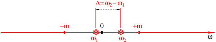
Figure 3: Two-point spectrum

The spectrum of this expression contains the harmonics with new frequencies $\omega_{1}-\Delta$ and $\omega_{2}+\Delta$. As a result, all the frequencies $\omega_{1}-\Delta$, $\omega_{1}-2\Delta,\dotsc$ and $\omega_{2}+\Delta$, $\omega_{2}+2\Delta$, $\dotsc$ will also appear in the dynamics (see Fig. 4)).

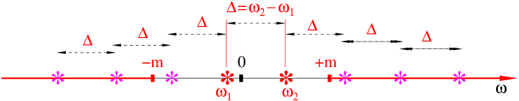
Figure 4: Nonlinear inflation of spectrum

Therefore, the frequency lying in the continuous spectrum $|\omega_{0}|\geq m$ will necessarily appear, causing the radiation of energy. This radiation will continue until the spectrum of the solution contains at least two different frequencies. Exactly this fact prohibits the presence of two different frequencies in omega-limit trajectories, because the finite energy solution cannot radiate indefinitely.

Let us emphasize that the spectrum inflation by polynomials is established by the Titchmarsh convolution theorem, since the Fourier transform of a product of functions equals the convolution of their Fourier transforms.

Remark 3.13.

Physically the arguments above suggest the following nonlinear radiation mechanism:
i) The nonlinearity inflates the spectrum which means the energy transfer from lower to higher modes;
ii) Then the dispersion radiation of the higher modes transports their energy to infinity.
We have justified this radiation mechanism for the first time for the nonlinear $U(1)$-invariant equations (3.1) and (3.13)–(3.15). Our numerical experiments confirm the same radiation mechanism for nonlinear relativistically-invariant wave equations, see Remark 7.1.

4 Global attraction to solitons

Here we describe the results of global attraction to solitons (1.9) for translation-invariant equations.

4.1 Translation-invariant wave-particle system

In [118], we considered the system (2.32)–(2.33) with zero potential $V=0$:

$$\left\{\begin{array}[]{rlrl}\dot{\psi}(x,t)\!\!&\!\!=\pi(x,t),&\dot{\pi}(x,t)\!\!&\!\!=\Delta\psi(x,t)-\rho(x-q(t)),\qquad x\in\mathbb{R}^{3}\\ \\ \dot{q}(t)\!\!&\!\!=\displaystyle\frac{p(t)}{\sqrt{1+p^{2}(t)}},&\dot{p}(t)\!\!&\!\!=-\displaystyle\int\nabla\psi(x,t)\rho(x-q(t))\,dx.\end{array}\right|$$ (4.1)

The corresponding Hamiltonian reads

$${\cal H}_{0}(\psi,\pi,q,p)=\displaystyle\frac{1}{2}\int[|\pi(x)|^{2}+|\nabla\psi(x)|^{2}]\,dx+\int\psi(x)\rho(x-q)\,dx+\sqrt{1+p^{2}},$$ (4.2)

which coincides with (2.36) for $V=0$. It is conserved along trajectories of the system (4.1). Furthermore, this system is translation-invariant, and the corresponding total momentum

$$P=p-\int\pi(x)\nabla\psi(x)\,dx.$$ (4.3)

is also conserved. The system (4.1) admits traveling wave solutions (solitons)

$$\left\{\begin{array}[]{rlrl}\psi_{v,a}(x,t)\!\!&\!\!=\psi_{v}(x-vt-a),&\pi_{v,a}(x,t)\!\!&\!\!=\pi_{v}(x-vt-a)\\ \\ q_{v,a}(t),\!\!&\!\!=vt+a&p_{v}\!\!&\!\!:=v/\sqrt{1-v^{2}}\end{array}\right|$$ (4.4)

where $v,a\in\mathbb{R}^{3}$ with $|v|<1$. The set of these solitons form a $6$-dimensional solitary submanifold in ${\cal E}$:

$${\cal S}=\{S_{v,a}=(\psi_{v}(x-a),\pi_{v}(x-a),a,p_{v}):\quad v,a\in\mathbb{R}^{3},\quad|v|<1\}$$ (4.5)

The main result of [118] is the following theorem.

Theorem 4.1.

Let the Wiener condition (2.40) hold. Then, for any finite energy solutions to the system (4.1),

$$\dot{q}(t)\xrightarrow[t\to\pm\infty]{}v_{\pm}.$$ (4.6)

Moreover, for the field components the soliton asymptotics hold,

$$(\psi(x,t),\pi(x,t))=(\psi_{v_{\pm}}(x-q(t)),\pi_{v_{\pm}}(x-q(t)))+(r_{\pm}(x,t),s_{\pm}(x,t))$$ (4.7)

where the remainders locally decay in the moving frame of the particle: for every $R>0$

$$\|\nabla r_{\pm}(q(t)+x,t)\|_{R}+\|r_{\pm}(q(t)+x,t)\|_{R}+\|s_{\pm}(q(t)+x,t)\|_{R}\xrightarrow[t\to\pm\infty]{}0.$$ (4.8)

The proof [118] relies on a) the relaxation of acceleration (2.44) which holds for $V=0$ (see Remark 2.7 i)), and b) on the canonical change of variables to the comoving frame. The key role plays the fact that the soliton $S_{v,a}$ minimizes the Hamiltonian (4.2) under fixed total momentum (4.3), implying the orbital stability of solitons [36, 37]. Furthermore, the strong Huygens principle for the 3D wave equation is used.

Remark 4.2.

The Wiener condition (2.40) is sufficient for the relaxation (2.44) of solutions to translation-invariant system  (4.1). However it is not necessary: for example, (2.44) obviously holds for $\rho(x)\equiv 0$. Moreover, (2.44) holds also in the case of small $\|\rho\|$, see Section 4.3.

4.2 Translation-invariant Maxwell-Lorentz equations

In [119], asymptotics of type (4.6)–(4.8) were extended to the translation-invariant Maxwell–Lorentz system (2.52) with zero external fields. In this case, the Hamiltonian (2.54) reads as

$${\cal H}_{0}=\frac{1}{2}\int[E^{2}(x)+B^{2}(x)]\,dx+\sqrt{1+p^{2}}.$$ (4.9)

The extension of the arguments [118] to this case required an essential analysis of the corresponding Hamiltonian structure which is necessary for the canonical transformation. Now the key role in application of the strong Huygens principle play novel estimates for the decay of oscillations of the Hamiltonian (4.9) and of total momentum along solutions to a perturbed Maxwell-Lorentz system, see [119, (4.24) and (4.25)].

4.3 Weak coupling

Asymptotics of type (4.6)–(4.8) in a stronger form were proved for the system (2.32)–(2.33) under the weak coupling condition

$$\|\rho\|_{L^{2}(\mathbb{R}^{3})}\ll 1.$$ (4.10)

Namely, in [120] we have considered initial fields with a decay $|x|^{-5/2-\sigma}$ with a parameter $\sigma>0$ (condition (2.2) of [120]), assuming that

$$\nabla V(q)=0,\qquad\qquad|q|>{\rm const}.$$ (4.11)

Under these assumptions we prove the strong relaxation

$$|\ddot{q}(t)|\leq C(1+|t|)^{-1-\sigma},\qquad t\in{\mathbb{R}}$$ (4.12)

for ”outgoing” solutions which satisfy the condition

$$|q(t)|\xrightarrow[t\to\pm\infty]{}\infty.$$ (4.13)

In particular, all solutions are outgoing in the case $V(q)\equiv 0$. Asymptotics (4.6)–(4.8) under these assumptions are refined similarly to (2.22):

$$\dot{q}(t)\to v_{\pm},~{}~{}(\psi(x,t),\pi(x,t))\!=\!(\psi_{v_{\pm}}(x\!-\!q(t)),\pi_{v_{\pm}}(x\!-\!q(t)))+W(t)\Phi_{\pm}+(r_{\pm}(x,t),s_{\pm}(x,t)),~{}~{}t\to\pm\infty.$$ (4.14)

Here the ‘dispersion waves’ $~{}W(t)\Phi_{\pm}$ are solutions to the free wave equation, and the remainder now converges to zero in the global energy norm:

$$\|\nabla r_{\pm}(q(t)+x,t)\|+\|r_{\pm}(q(t)+x,t)\|+\|s_{\pm}(q(t)+x,t)\|\xrightarrow[t\to\pm\infty]{}0.$$ (4.15)

Remark 4.3.

This progress with respect to the local decay (4.8) is due to the fact that we identify the dispersion wave $W(t)\Phi_{\pm}$ under the smallness condition (4.10). This identification is possible by the decay rate (4.12) which is more strong than (2.44).

The solitons propagate with velocities less than $1$, and therefore they separate at large time from the dispersion waves $W(t)\Phi_{\pm}$, which propagate with unit velocity (Fig. 5).

The proofs rely on the integral Duhamel representation and rapid dispersion decay for the free wave equation. A similar result was obtained in [121] for a system of type (2.32)–(2.33) with the Klein–Gordon equation, and in [122], for the system (2.52) under the same condition (4.13) assuming that $E^{\rm ext}(x)=B^{\rm ext}(x)=0$ for $|x|>{\rm const}$. In [123], this result was extended to a system of type (2.52) with a rotating charge in the Maxwell field.

Remark 4.4.

The results [120]–[123] imply the ”Grand Conjecture” [57, p.460] in the moving frame for the corresponding systems with $V(q)\equiv 0$ and $E^{\rm ext}(x)\equiv B^{\rm ext}(x)\equiv 0$ under the smallness condition (4.10).

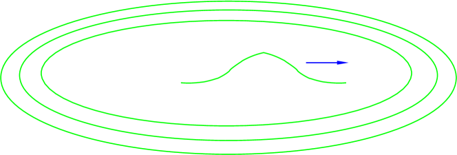
Figure 5: Soliton and dispersion waves

4.4 Solitons of relativistically-invariant equations

The existence of soliton solutions $\psi(x-vt)$ was extensively studied in the 1960–1980’s for a wide class of relativistically-invariant $U(1)$-invariant nonlinear wave equations

$$\ddot{\psi}(x,t)=\Delta\psi(x,t)+F(\psi(x,t)),\qquad x\in\mathbb{R}^{n}.$$ (4.16)

Here $F(\psi)=-\nabla_{\overline{\psi}}U(\psi)$, where $U(\psi)=u(|\psi|)$ with $u\in C^{2}(\mathbb{R})$. In this case, equation (4.16) is equivalent to the Hamilton system of type (2.8) with a conserved in time Hamilton functional

$${\cal H}(\psi,\pi)=\int[\frac{1}{2}|\pi(x)|^{2}+\frac{1}{2}|\nabla\psi(x)|^{2}+U(\psi(x))]\,dx.$$ (4.17)

This equation is translation-invariant, so the total momentum

$$P:=-\int\pi(x)\nabla\psi(x)\,dx$$ (4.18)

is also conserved. Furthermore, this equation is also $U(1)$-invariant; i.e., $F(e^{-i\theta}\psi)\equiv e^{i\theta}F(\psi)$ for $\theta\in[0,2\pi]$. Respectively, it can admit soliton solutions of the form $e^{-i\omega t}\phi_{\omega}(x)$. Substitution into (4.16) gives the nonlinear eigenfunction problem

$$-\omega^{2}\phi_{\omega}(x)=\Delta\phi_{\omega}(x)+F(\phi_{\omega}(x)),\qquad x\in\mathbb{R}.$$ (4.19)

Under suitable conditions on the potential $U$, solutions $\phi_{\omega}\in H^{1}(\mathbb{R}^{n})$ exist and decay exponentially as $|x|\to\infty$ for $\omega\in{\cal O}$, where ${\cal O}$ is an open subset of $\mathbb{R}$.

The most general results on the existence of the solitons were obtained by Strauss, Berestycki and P.-L. Lions [30, 31, 32]. The approach [32] relies on variational and topological methods of the Ljusternik–Schnirelman theory [33, 34]. The development of this approach in [35] provided the existence of solitons for nonlinear relativistically-invariant Maxwell–Dirac equations (A.6).

The orbital stability of solitons has been studied by Grillakis, Shatah, Strauss, and others [36, 37]. However, the global attraction to solitons (1.10) is still open problem.

The equation (4.16) is also Lorentz-invariant. Hence, the solitons with any velocities $|v|<1$ are obtained from the ‘standing soliton’ $e^{-i\omega t}\phi_{\omega}(x)$ via the Lorentz transformation

$$\psi_{v,\omega}(x,t):=e^{-i\omega\gamma_{v}(t-vx)}\phi_{\omega}(\gamma_{v}(x-vt)),\qquad\gamma_{v}:=\sqrt{1-v^{2}}.$$ (4.20)

The total energy (4.17) and the total momentum (4.18) of the soliton coincide with the corresponding formulas for a relativistic particle (see [125, (4.1)]):

$$E_{v,\omega}=\displaystyle\frac{m_{0}(\omega)}{\sqrt{1-v^{2}}},\qquad P_{v,\omega}=\displaystyle\frac{m_{0}(\omega)v}{\sqrt{1-v^{2}}},$$ (4.21)

where $m_{0}(\omega)>0$ for $\omega\neq 0$, provided (3.4) holds. Therefore, the relativistic ‘dispersion relation’ holds,

$$E_{v,\omega}^{2}=m_{0}^{2}(\omega)+P_{v,\omega}^{2},$$ (4.22)

which implies the Einstein’s famous formula $E=m_{0}c^{2}$ if $v=0$ (recall that we set $c=1$).

In the one-dimensional case $n=1$, equation (4.19) reads

$$-\omega^{2}\phi_{\omega}(x)=\phi_{\omega}^{\prime\prime}(x)+F(\phi_{\omega}(x)),\qquad x\in\mathbb{R}.$$ (4.23)

This ordinary differential equation is easily solved in quadratures using the ‘energy integral’

$$\frac{1}{2}|\phi_{\omega}^{\prime}(x)|^{2}-U(\phi_{\omega}(x))+\frac{1}{2}\omega^{2}|\phi_{\omega}(x)|^{2}={\rm const},\qquad x\in\mathbb{R}.$$ (4.24)

Figure 6: The potential $U$

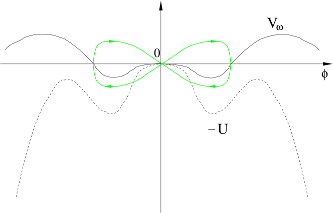
Figure 7: Potentials and soliton on the phase plane

This identity shows that finite energy solutions to the equation (4.24) exist for potentials $U$, similar to shown in Fig. 6. Namely, the potential $V_{\omega}(\phi):=-U(\phi)+\frac{1}{2}\omega^{2}|\phi|^{2}$ with $\omega^{2}<U^{\prime\prime}(0)$ has the shape represented in Fig. 7, guarantying the existence of an exponentially decaying trajectory as $x\to\pm\infty$ (the green contour) which represents the soliton.

5 Adiabatic effective dynamics of solitons

Existence of solitons and soliton-type asymptotics (4.7) are typical features of translation-invariant systems. However, if a deviation of a system from translation invariance is small in some sense, then the system may admit solutions that are permanently close to solitons with parameters depending on time (velocity, etc.). Moreover, in some cases it turns out possible to find an ‘effective dynamics’ describing the evolution of these parameters.

5.1 Wave-particle system with slowly varying external potential

Solitons (4.4) are solutions to the system (4.1) with zero external potential. However, even for the corresponding system (2.32)–(2.33) with a nonzero external potential the soliton-like solutions of the form

$$\psi(x,t)\approx\psi_{v(t)}(x-q(t))$$ (5.1)

may exist if the potential is slowly varying:

$$|\nabla V(q)|\leq\varepsilon\ll 1.$$ (5.2)

Now the total momentum (4.3) is not conserved, but its slow evolution together with evolution of solutions (5.1) can be described in terms of finite-dimensional Hamiltonian dynamics.

Let us denote by $P=P_{v}$ the total momentum of the soliton $S_{v,Q}$ in the notations (4.5), and observe that the mapping ${\cal P}:v\mapsto P_{v}$ is an isomorphism of the ball $|v|<1$ onto $R^{3}$. Therefore, we can regard $Q,P$ as the global coordinates on the solitary manifold ${\cal S}$ and define an effective Hamilton functional

$$H_{\rm eff}(Q,P_{v})\equiv{\cal H}_{0}(S_{v,Q}),\qquad(Q,P_{v})\in{\cal S},$$ (5.3)

where ${\cal H}_{0}$ is the unperturbed Hamiltonian (4.2). It is easy to observe that the functional admits the splitting $H_{\rm eff}(Q,\Pi)=E(\Pi)+V(Q)$, so that the corresponding Hamilton equations read

$$\dot{Q}(t)=\nabla E(\Pi(t)),\qquad\dot{\Pi}(t)=-\nabla V(Q(t)).$$ (5.4)

The main result of [132] is the following theorem.

Theorem 5.1.

Let condition (5.2) hold, and let the initial state $(\psi_{0},\pi_{0},q_{0},p_{0})$ be a soliton $S_{0}\in{\cal S}$ with total momentum $P_{0}$. Then the corresponding solution $(\psi(x,t),\pi(x,t),q(t),p(t))$ to the system (2.32)–(2.33) admits the following ‘adiabatic asymptotics’

$$|q(t)-Q(t)|\leq C_{0},\quad|P(t)-\Pi(t)|\leq C_{1}\varepsilon\quad\mbox{\rm for}\quad|t|\leq C\varepsilon^{-1},$$ (5.5)

$$\sup_{t\in\mathbb{R}}\Big{[}\|\nabla[\psi(q(t)+x,t)-\psi_{v(t)}(x)]\|_{R}+\|\pi(q(t)+x,t)-\pi_{v(t)}(x)]\|_{R}\Big{]}\leq C\varepsilon,$$ (5.6)

where $P(t)$ is the total momentum (4.3), the velocity $v(t)={\cal P}^{-1}(\Pi(t))$, and $(Q(t),\Pi(t))$ is the solution to the effective Hamilton equations (5.4) with initial conditions

$$Q(0)=q(0),\qquad\Pi(0)=P(0).$$ (5.7)

Note that the relevance of effective dynamics (5.4) is due to consistency of the Hamilton structures:
1) The effective Hamiltonian (5.3) is the restriction of the Hamiltonian (4.2) onto the solitary manifold ${\cal S}$.
2) As shown in [132], the canonical form of the Hamilton system (5.4) is also the restriction of the canonical form of the original system (2.32)–(2.33) onto ${\cal S}$:

$$P\,dQ=\Bigl{[}p\,dq+\int\psi(x)\,d\pi(x){\hskip 1.42262pt}dx\Bigr{]}\Big{|}_{\cal S}.$$ (5.8)

Hence, the total momentum $P$ is canonically conjugate to the variable $Q$ on the solitary manifold ${\cal S}$. This fact clarifies definition (5.3) of the effective Hamilton functional as the function of the total momentum $P_{v}$, rather than of the particle momentum $p_{v}$.

One of main results of [132] is the following ‘effective dispersion relation’:

$$E(\Pi)\sim\frac{\Pi^{2}}{2(1+m_{e})}+{\rm const},\qquad|\Pi|\ll 1.$$ (5.9)

It means that the non-relativistic mass of the slow soliton increases due to the interaction with the field by the value

$$m_{e}=-\frac{1}{3}\langle\rho,\Delta^{-1}\rho\rangle.$$ (5.10)

This increment is proportional to the field-energy of the soliton at rest, that agrees with the Einstein principle of the mass-energy equivalence (see below).

Remark 5.2.

The relation (5.9) suggests only a hint that $m_{e}$ is the increment of the effective mass. The genuine justification is given by relevance of the adiabatic effective dynamics (5.4) which is confirmed by the asymptotics (5.5)–(5.6).

5.2 Generalizations and the mass-energy equivalence

In [133], asymptotics (5.5), (5.6) were extended to solitons of the Maxwell–Lorentz equations (2.52) with small external fields, and the increment of the non-relativistic mass of type (5.10) was calculated. It also turns out to be proportional to the own field energy of the static soliton.

Such an equivalence of the own electromagnetic field energy of the particle and of its mass was first suggested in 1902 by Abraham: he obtained by a direct calculation that the electromagnetic self-energy $E_{\rm own}$ of the electron at rest contributes the increment $m_{e}=\displaystyle\frac{4}{3}E_{\rm own}/c^{2}$ into its nonrelativistic mass (see [127, 128], and also [10, pp. 216–217]). It is easy to see that this self-energy is infinite for the point electron with the charge density $\delta(x-q)$, because in this instance the Coulomb electrostatic field $|E(x)|\sim C/|x-q|^{2}$ as $x\to q$, so that the integral in (2.54) diverges. Respectively, the field mass for a point electron is infinite, which contradicts the experiment. This is why Abraham introduced the model of ‘extended electron’ for which the self-energy is finite.

At that time Abraham put forth the idea that the whole mass of an electron is due to its own electromagnetic energy; i.e., $m=m_{e}$: ‘… the matter has disappeared, only the radiation remains…’, as wrote philosophically minded contemporaries [130, pp. 63, 87, 88] (Smile :) )

This idea was refined and developed in 1905 by Einstein, who has discovered the famous universal relation $E=m_{0}c^{2}$ suggested by the relativity theory [129]. The extra factor $\frac{4}{3}$ in the Abraham formula is due to the non-relativistic nature of the system (2.52). According to the modern view, about 80 % of the electron mass has electromagnetic origin [131].

Further, the asymptotics of type (5.5), (5.6) were obtained in [134, 135] for the nonlinear Hartree and Schrödinger equations with slowly varying external potentials, and in [136]–[138], for nonlinear Einstein–Dirac, Chern–Simon–Schrödinger and Klein–Gordon-Maxwell equations with small external fields.

Recently, a similar adiabatic effective dynamics was established in [139] for an electron in the second-quantized Maxwell field in presence of a slowly varying external potential.

Remark 5.3.

The dispersion relation (4.22) for relativistic solitons formally implies the Einstein’s formula $E=m_{0}c^{2}$ if $v=0$ (recall that we set $c=1$). However, its genuine dynamical justification requires the relevance of the corresponding adiabatic effective dynamics for the solitons with the relativistic kinetic energy $E=\sqrt{m_{0}^{2}+P^{2}}$. The first result of this type for relativistically-invariant Klein–Gordon-Maxwell equations is established in [138].

6 Asymptotic stability of solitary waves

The asymptotic stability of solitary manifolds means the local attraction; i.e., for the state sufficiently close to the manifold. The main peculiarity of this attraction is the instability of the dynamics along the manifold. This follows directly from the fact that the solitary waves move with different velocities, and therefore run away over a long time.

Analytically, this instability is related to the presence of the discrete spectrum of the linearized dynamics with ${\rm Re{\hskip 1.42262pt}{\hskip 1.42262pt}}\lambda\geq 0$. Namely, the tangent vectors to the solitary manifolds are the eigenvectors and the associated eigenvectors of the generator of the linearized dynamics at the solitary wave. They correspond to the zero eigenvalue. Respectively, the Lyapunov theory is not applicable in this case.

In a series of papers an ingenious strategy was developed for proving the asymptotic stability of solitary manifolds. In particular, this strategy includes the symplectic projection of the trajectory onto the solitary manifold, the modulation equations for the soliton parameters of the projection, and the decay of the transversal component. This approach is a far-reaching development of the Lyapunov stability theory.

6.1 Linearization and decomposition of the dynamics

The strategy was initiated in the pioneering works of Soffer and Weinstein [51, 52, 53]; see the survey [57]. The results concern the nonlinear $U(1)$-invariant Schrodinger equation with a real potential $V(x)$

$$i\dot{\psi}(x,t)=-\Delta\psi(x,t)+V(x)\psi(x,t)+\lambda|\psi(x,t)|^{p}\psi(x,t),\qquad x\in\mathbb{R}^{n},$$ (6.1)

where $\lambda\in\mathbb{R}$, $p=3$ or $4$, $n=2$ or $n=3$, and $\psi(x,t)\in{\mathbb{C}}$. The corresponding Hamilton functional reads

$$H=\int[\frac{1}{2}|\nabla\psi|^{2}+\frac{1}{2}V(x)|\psi(x)|^{2}+\frac{\lambda}{p}|\psi(x)|^{p}]\,dx.$$ (6.2)

For $\lambda=0$ the equation (6.1) is linear. Let $\phi_{*}(x)$ denote its ground state corresponding to the minimal eigenvalue $\omega_{*}<0$. Then $C\phi_{*}(x)e^{-i\omega_{*}t}$ are periodic solutions for any complex constant $C$. The corresponding phase curves are the circles filling the complex line (which is the real plane). For nonlinear equations (6.1) with small real $\lambda\neq 0$, it turns out that a remarkable bifurcation occurs: a small neighborhood of zero of the complex line is transformed into an analytic-invariant solitary manifold ${\cal S}$ which is still filled by the circles $\psi_{\omega}(x)e^{-i\omega t}$ with frequencies $\omega$ close to $\omega_{*}$.

The main result of [52, 53] (see also [54]) is the long time attraction to one of these trajectories at large times for any solution with sufficiently small initial data

$$\psi(x,t)=\psi_{\pm}(x)e^{-i\omega_{\pm}t}+r_{\pm}(x,t),$$ (6.3)

where the remainder decays in the weighted norms: for $\sigma>2$

$$\|\langle x\rangle^{-\sigma}r_{\pm}(\cdot,t)\|_{L^{2}(\mathbb{R}^{n})}\xrightarrow[t\to\pm\infty]{}0,$$ (6.4)

where $\langle x\rangle:=(1+|x|)^{1/2}$. The proofs rely on linearization of the dynamics, the decomposition

$$\psi(t)=e^{-i\Theta(t)}(\psi_{\omega(t)}+\phi(t)),$$

and the orthogonality condition

$$\langle\psi_{\omega(0)},\phi(t)\rangle=0$$ (6.5)

(see [52, (3.2) and (3.4)]). This orthogonality and the dynamics (6.1) imply the modulation equations for $\omega(t)$ and $\gamma(t)$ where $\gamma(t):=\Theta(t)-\displaystyle\int_{0}^{t}\omega(s)ds$ (see (3.2) and (3.9a), (3.9b) of [52]. The orthogonality (6.5) ensures that $\phi(t)$ lies in the continuous spectral space of the Schrödinger operator $H(\omega_{0}):=-\Delta+V+\lambda|\psi_{\omega_{0}}|^{m-1}$ which results in the time decay [52, (4.2a) and (4.2b)] of the component $\phi(t)$. Finally, this decay implies the convergence $\omega(t)\to\omega_{\pm}$ and the asymptotics (6.3) as $t\to\pm\infty$.

These results and methods were further developed by many authors for nonlinear Schrödinger, wave and Klein–Gordon equations with external potentials under various types of spectral assumptions on the linearized dynamics [54] - [60] for the case of small inital data.

A significant progress in this theory has been achieved by Buslaev, Perelman and Sulem who have established in [63]–[65] the asymptotics of type (6.3) for the first time for translation-invariant 1D Schrödinger equations

$$i\dot{\psi}(x,t)=-\psi^{\prime\prime}(x,t)+F(\psi(x,t)),\qquad x\in\mathbb{R}$$ (6.6)

which are also $U(1)$-invariant. The latter means that the nonlinear function $F(\psi)$ satisfies the identities (3.6)–(3.8). Then the corresponding solitons have the form $\psi(x,t)=\psi_{v,\omega}(x-vt-a)e^{-i(\omega t+\theta)}$. The set of all solitons form 4-dimensional smooth submanifold ${\cal S}$ of the Hilbert phase space ${\cal X}:=L^{2}({\mathbb{R}})$.

The novel approach [63]–[65] relies on the symplectic projection $P$ of solutions onto the solitary manifold. This means that for $S:=P\psi$ we have

$$Z:=\psi-S\quad\mbox{is symplectic-orthogonal to the tangent space}\quad{\cal T}:=T_{S}{\cal S}.$$ (6.7)

The projection is well defined in a small neighborhood of ${\cal S}$: it is important that ${\cal S}$ is the symplectic manifold, i.e. the symplectic form is nondegenerate on the tangent spaces $T_{S}{\cal S}$. Now the solution is decomposed into the symplectic orthogonal components $\psi(t)=S(t)+Z(t)$ where $S(t):=P\psi(t)$, and the dynamics is linearized at the solitary wave $S(t):=P\psi(t)$ for every $t>0$. In particular, the approach [63]–[65] allowed to get rid of the smallness assumption on initial data.

The main results of [63]–[65] are the asymptotics of type (4.14), (6.3) for solutions with initial data close to the solitary manifold ${\cal S}$:

$$\psi(x,t)=\psi_{\pm}(x-v_{\pm}t)e^{-i\omega_{\pm}t}+W(t)\Phi_{\pm}+r_{\pm}(x,t),$$ (6.8)

where $W(t)$ is the dynamical group of the free Schrödinger equation, $\Phi_{\pm}$ are some finite energy states, and $r_{\pm}$ are the remainders which tend to zero in the global norm:

$$\|r_{\pm}(\cdot,t)\|_{L^{2}(\mathbb{R})}\xrightarrow[t\to\pm\infty]{}0.$$ (6.9)

The asymptotics are obtained under the condition [65, (1.0.12)] which means the strong coupling of the discrete and continuous spectral components. This condition is the nonlinear version of the Fermi Golden Rule [89] which was originally introduced by Sigal [90, 91]. In [68], these results were extended to nD translation-invariant Schrödinger equations in dimensions $n\geq 2$.

6.2 Method of symplectic projection in the Hilbert space

The proofs of asymptotics (6.8)–(6.9) in [63]–[65] rely on the linearization of the dynamics (6.6) at the soliton $S(t):=P\psi(t)$ which is the nonlinear symplectic projection of $\psi(t)$ onto the solitary manifold ${\cal S}$. The Hilbert phase space ${\cal X}:=L^{2}({\mathbb{R}})$ admits the splitting ${\cal X}={\cal T}(t)\oplus{\cal Z}(t)$, where ${\cal Z}(t)$ is the symplectic orthogonal space to the tangent space ${\cal T}(t):=T_{S(t)}{\cal S}$. The corresponding equation for the transversal component $Z(t)$ reads

$$\dot{Z}(t)=A(t)Z(t)+N(t),$$ (6.10)

where $A(t)Z(t)$ is the linear part while $N(t)={\cal O}(\|Z(t)\|^{2})$ is the corresponding nonlinear part. The main peculiarity of this equation is that it is nonautonomous, and the generators $A(t)$ are nonselfadjoint (see Appendix [82]). The main issue is that $A(t)$ are Hamiltonian operators. The strategy of [63]–[65] relies on the following ideas.
S1. Modulation equations. The parameters of the soliton $S(t)$ satisfy modulation equations: for example, for its velocity we have $\dot{v}(t)=M(\psi(t))$, where $M(\psi)={\cal O}(\|Z\|^{2})$ for small $\|Z\|$. Hence, the parameters vary extra slowly near the solitary manifold, like adiabatic invariants.
S2. Tangent and transversal components. The transversal component $Z(t)$ in the splitting $\psi(t)=S(t)+Z(t)$ belongs to the transversal space ${\cal Z}(t)$. The tangent space ${\cal T}(t)$ is the root space of $A(t)$ which corresponds to the ”unstable” spectral point $\lambda=0$. The key observation is that i) the symplectic-orthogonal space ${\cal Z}(t)$ does not contain the ”unstable” tangent vectors, and moreover, ii) ${\cal Z}(t)$ is invariant under the generator $A(t)$ since ${\cal T}(t)$ is invariant and $A(t)$ is the Hamiltonian operator.
S3. Continuous and discrete components. The transversal component admits further splitting $Z(t)=z(t)+f(t)$, where $z(t)$ and $f(t)$ belong respectively to the discrete and continuous spectral spaces ${\cal Z}_{d}(t)$ and ${\cal Z}_{c}(t)$ of the generator $A(t)$ in the invariant space ${\cal Z}(t)={\cal Z}_{d}(t)+{\cal Z}_{c}(t)$.
S4. Elimination of continuous component. Equation (6.10) can be projected onto ${\cal Z}_{d}(t)$ and ${\cal Z}_{c}(t)$. Then the continuous transversal component $f(t)$ can be expressed via $z(t)$ and the terms ${\cal O}(\|f(t))\|^{2}$ from the projection onto ${\cal Z}_{c}(t)$. Substituting this expression into the projection onto ${\cal Z}_{d}(t)$, we obtain a nonlinear cubic equation for $z(t)$ which includes also ‘higher order terms’ ${\cal O}([\|f(t))\|+|z(t)|^{2}]^{2})$: see equations (3.2.1)-(3.2.4) and (3.2.9)-(3.2.10) of [65]. (For relativistically-invariant Ginzburg-Landau equation similar reduction has been done in [79, (4.9) and (4.10)].)
S5. Poincaré normal forms and Fermi Golden Rule. Neglecting the higher order terms, the equation for $z(t)$ reduces to the Poincaré normal form which implies the decay for $z(t)$ due to the ‘Fermi Golden Rule’ [65, (1.0.12)].
S6. Method of majorants. A skillful interplay between the obtained decay and the extra slow evolution of the soliton parameters S1 provides the decay for $f(t)$ and $z(t)$ by the method of majorants. This decay immediately results in the asymptotics (6.8)-(6.9).

6.3 Development and applications

In [61, 62], these methods and results were extended i) to the Schrödinger equation interacting with nonlinear $U(1)$-invariant oscillators, ii) in [72, 75], to the system (4.1) and to (2.52) with zero external fields, and iii) in [71, 73, 74], to similar translation-invariant systems of Klein–Gordon, Schrödinger and Dirac equations coupled to a particle. A survey of the results [71, 72, 75] can be found in [76].

For example, in [75] we have considered solutions to the system (4.1) with initial data close to the solitary manifold (4.4) in the weighted norm

$$\|\psi\|_{\sigma}^{2}=\int\langle x\rangle^{2\sigma}|\psi(x)|^{2}dx.$$ (6.11)

Namely, the initial state is close to soliton (4.4) with some parameters $v_{0},a_{0}$:

$$\begin{gathered}\|\nabla\psi(x,0)-\nabla\psi_{v_{0}}(x-a_{0})\|_{\sigma}+\|\psi(x,0)-\psi_{v_{0}}(x-a_{0})\|_{\sigma}+\|\pi(x,0)-\pi_{v_{0}}(x-a_{0})\|_{\sigma}\\ +|q(0)-a_{0}|+|\dot{q}(0)-v_{0}|\leq\varepsilon,\end{gathered}$$ (6.12)

where $\sigma>5$ and $\varepsilon>0$ are sufficiently small. Moreover, we assume the Wiener condition (2.40) for $k\neq 0$, while

$$\partial^{\alpha}\hat{\rho}(0)=0,\quad|\alpha|\leq 5;$$ (6.13)

this is equivalent to

$$\int x^{\alpha}\rho(x)\,dx=0,\quad|\alpha|\leq 5.$$ (6.14)

Under these conditions, the main results of [75] are the following asymptotics:

$$\dot{q}(t)\to v_{\pm},\quad q(t)\sim v_{\pm}t+a_{\pm},\qquad t\to\pm\infty$$ (6.15)

(cf. (4.6)). Moreover, the attraction to solitons (4.7) holds, where the remainders now decay in the weighted norm in the moving frame of the particle (cf. (4.8)):

$$\|\nabla r_{\pm}(q(t)+x,t)\|_{-\sigma}+\|r_{\pm}(q(t)+x,t)\|_{-\sigma}+\|s_{\pm}(q(t)+x,t)\|_{-\sigma}\xrightarrow[t\to\pm\infty]{}0.$$ (6.16)

In [77]–[80] and [83], the methods and results [63]–[65] were extended to relativistically-invariant nonlinear equations. Namely, in [77]–[80] the asymptotics of type (6.8) were obtained for the first time for the relativistically-invariant nonlinear Ginzburg–Landau equations, and in [83], for relativistically-invariant nonlinear Dirac equations. In [81], we have constructed examples of Ginzburg–Landau type potentials providing the spectral properties of the linearized dynamics imposed in [77]–[80]. In [82], we have justified the eigenfunction expansions for nonselfadjoint Hamiltonian operators which were used in [77]–[80]. For the justification we have developed a special version of M.G. Krein theory of $J$-selfadjoint operators.

In [84], the system of type (4.1) with the Schrödinger equation instead of the wave equation is considered as a model of the Cherenkov radiation of a tracer particle (the system (1.9)–(1.10) of [84]). The main result of [84] is the long time convergence to a soliton with a subsonic speed for initial solitons with supersonic speeds. The asymptotic stability of the solitons for similar system has been established in [73].

Asymptotic stability of $N$-soliton solutions to nonlinear translation-invariant Schrödinger equations was studied in [85]–[88] by developing the methods of [63]–[65].

Remark 6.1.

The asymptotics (6.15)–(6.16) mean the proximity of the trajectory to the solitary manifold in the weighted norms under the proximity of the corresponding initial state (6.12) and under the Wiener condition (2.40). The Wiener condition implies also the global attraction to solitons (4.6)–(4.8). This could suggest an impression that the Wiener condition provides the proximity to the solitary manifold (6.12) for large times. However, this impression is erroneous since the decay (4.8) implies the proximity in the local energy seminorms which is weaker than the proximity in the weighted norms (6.12).

7 Numerical simulation of soliton asymptotics

Here we describe the results of our joint work with Arkady Vinnichenko (1945–2009) on numerical simulation of the global attraction to solitons (1.9) and (1.10), and adiabatic effective soliton-type dynamics (5.6) for the relativistically-invariant one-dimensional nonlinear wave equations [124].

7.1 Kinks of relativistically-invariant Ginzburg–Landau equation

We have considered real solutions to the relativistically-invariant 1D Ginzburg–Landau equation, which is the nonlinear Klein–Gordon equation with polynomial nonlinearity

$$\ddot{\psi}(x,t)=\psi^{\prime\prime}(x,t)+F(\psi(x,t)),\qquad\mbox{where}\quad F(\psi):=-\psi^{3}+\psi.$$ (7.1)

Since $F(\psi)=0$ for $\psi=0,\pm 1$, there are three equilibrium positions $S(x)\equiv 0,+1,-1$.

The corresponding potential reads $U(\psi)=\frac{\psi^{4}}{4}-\frac{\psi^{2}}{2}$. This potential has minimum at $\pm 1$ and maximum at 0, so the two equilibria are stable, and one is unstable. Such potentials with two wells are called the Ginzburg–Landau potentials.

Besides constant stationary solutions $S(x)\equiv 0,+1,-1$, there is still a non-constant steady-state ”kink” solution $S(x)=\tanh\frac{x}{\sqrt{2}}$. Its shifts and reflections $\pm S(x-a)$ are also stationary solutions, as well as their Lorentz transformations $\pm S(\gamma(x-a-vt))$ with $\gamma=\frac{1}{\sqrt{1-v^{2}}}$ for $|v|<1$. These are uniformly moving waves (i.e., solitons). When the velocity $v$ is close to $\pm 1$, this kink is very compressed.

Equation (7.1) is equivalent to the Hamiltonian system of form (2.8) with the Hamilton functional

$${\cal H}(\psi,\pi)=\int[\frac{1}{2}|\pi(x)|^{2}+\frac{1}{2}|\psi^{\prime}(x)|^{2}+U(\psi(x))]\,dx$$ (7.2)

defined on the Hilbert phase space ${\cal E}$ of states $(\psi,\pi)$ with the norm (2.6), for which

$$\psi(x)\xrightarrow[|x|\to\infty]{}\pm 1.$$

Our numerical experiments show the decay of finite energy solutions to a finite collection of kinks and a dispersion wave that confirms the asymptotics (1.10). One of the simulations is shown on Fig. 8: the considered finite energy solution to equation (7.1) decays to three kinks. Here, the vertical line is the time axis and the horizontal line is the space axis. The spatial scale redoubles at $t=20$ and $t=60$.

The red color corresponds to values $\psi>1-\varepsilon$, the blue one, to values $\psi<-1+\varepsilon$, and the yellow one, to values $-1+\varepsilon<\psi<1+\varepsilon$. Thus, the yellow stripes represents the kinks, while the blue and red zones outside the yellow stripes are filled with the dispersion waves $W(t)\Phi_{+}$.

At $t=0$ the solution starts from a fairly chaotic behavior when there are no kinks. After 20 seconds, there are three distinct kinks, which further move almost uniformly.

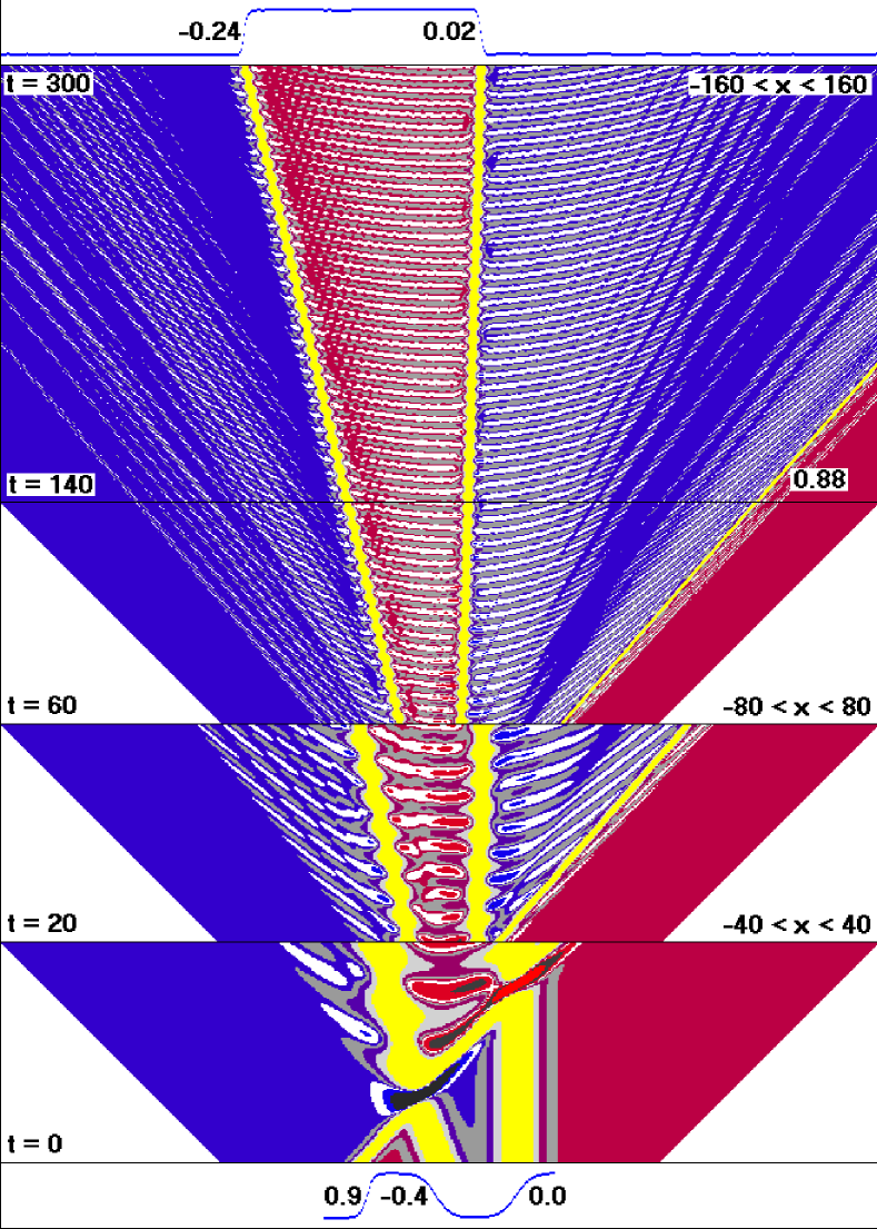
Figure 8: Decay to three kinks

The left kink moves to the left with small velocity $v_{1}\approx 0.24$, the central kink is almost standing with the velocity $v_{2}\approx 0.02$, and the right kink is very fast with velocity $v_{3}\approx 0.88$. The Lorentz contraction $\sqrt{1-v_{k}^{2}}$ is clearly visible on this picture: the central kink is wide, the left one is slightly narrower, and the right one is quite narrow.

Furthermore, the Einstein time delay here is also very pronounced. Namely, all three kinks oscillate due to presence of a nonzero eigenvalue in the linearized equation on the kink: substituting $\psi(x,t)=S(x)+\varepsilon\varphi(x,t)$ into (7.1) we obtain

$$\ddot{\varphi}(x,t)=\varphi^{\prime\prime}(x,t)-2\varphi(x,t)-V(x)\varphi(x,t)$$

in the first order the linearized equation, where the potential

$$V(x)=3S^{2}(x)-3=-\frac{3}{\cosh^{2}\frac{x}{\sqrt{2}}}$$

exponentially decays for large $|x|$. It is a great joy that for this potential the spectrum of the corresponding Schrödinger operator $H:=-\frac{d^{2}}{dx^{2}}+2+V(x)$ is well known [126]. Namely, the operator $H$ is non-negative, and its continuous spectrum coincides with $[2,\infty)$. It turns out that $H$ still has a two-point discrete spectrum: the points $\lambda=0$ and $\lambda=\frac{3}{2}$. These pulsation, which we observe for the central slow kink, have frequency $\omega_{1}\approx\sqrt{\frac{3}{2}}$ and period $T_{1}\approx 2\pi/\sqrt{\frac{3}{2}}\approx 5$ s. On the other hand, for the fast kink the ripples are much slower; i.e., the corresponding period is larger. This time delay agrees with the Lorentz formulas.

These agreements confirm the relevance of our numerical simulations of the solitons. Moreover, an analysis of the dispersion waves gives additional confirmations. Namely, the space outside the kinks in Fig. 8 is filled with dispersion waves, whose values are very close to $\pm 1$, with the accuracy $0.01$. The waves satisfy, with high accuracy, the linear Klein–Gordon equation, which is obtained by linearization of the Ginzburg–Landau equation (7.1) on the stationary solutions $\psi=\pm 1$:

$$\ddot{\varphi}(x,t)=\varphi^{\prime\prime}(x,t)+2\varphi(x,t).$$

The corresponding dispersion relation $\omega^{2}=k^{2}+2$ defines the group velocities of the wave packets,

$$\nabla\omega=\frac{k}{\sqrt{k^{2}+2}}=\pm\frac{\sqrt{\omega^{2}-2}}{\omega}$$ (7.3)

which are clearly seen in Fig. 8 as straight lines whose propagation velocities approach $\pm 1$. This approach is explained by the limit $|\nabla\omega|\to 1$ for high frequencies $\omega=\pm n\omega_{1}\to\infty$ generated by the polynomial nonlinearity in (7.1).

Remark 7.1.

These observations agree completely with the radiation mechanism summarized in Remark 3.13.

The nonlinearity in (7.1) is chosen so as to have well-known spectrum of the linearized equation. In the numerical experiments [124] we have considered more general nonlinearities, and the results were qualitatively the same: for ‘any’ initial data the solution again splits into a sum of solitons. Numerically, this can be clearly visible, but the rigorous justification is still the matter for the future.

7.2 Numerical observation of soliton asymptotics

Besides the kinks our numerical experiments [124] have also resulted in the soliton-type asymptotics (1.10) and adiabatic effective dynamics of type (5.6) for complex solutions to the 1D relativistically-invariant nonlinear wave equations (4.16). Namely, we have considered the polynomial potentials of the form

$$U(\psi)=a|\psi|^{2m}-b|\psi|^{2n},$$ (7.4)

where $a,b>0$ and $m>n=2,3,\dotsc$. Respectively,

$$F(\psi)=2am|\psi|^{2m-2}\psi-2bn|\psi|^{2n-2}\psi.$$ (7.5)

The parameters $a,b,m,n$ were taken as follows:

$$\begin{array}[]{rrrlr}N{}{}{}{}{}&a{}{}{}{}{}&~{}~{}~{}~{}m&~{}~{}~{}~{}~{}~{}b&~{}~{}~{}~{}n\\ 1{}{}{}{}{}&1{}{}{}{}&~{}~{}~{}~{}3&~{}~{}~{}~{}~{}~{}0.61&~{}~{}~{}~{}2\\ 2{}{}{}{}{}&10{}{}{}{}&~{}~{}~{}~{}4&~{}~{}~{}~{}~{}~{}2.1&~{}~{}~{}~{}2\\ 3{}{}{}{}{}&10{}{}{}{}&~{}~{}~{}~{}6&~{}~{}~{}~{}~{}~{}8.75&~{}~{}~{}~{}5\end{array}$$

We have considered various ‘smooth’ initial functions $\psi(x,0),\dot{\psi}(x,0)$ with the support on the interval $[-20,20]$. The second order finite-difference scheme with $\Delta x,\Delta t\sim 0.01,0.001$ was employed. In all cases we have observed the asymptotics of type (1.10) with the numbers of solitons $0,1,3$ for $t>100$.

7.3 Adiabatic effective dynamics of relativistic solitons in external potential

In the numerical experiments [124] was also observed the adiabatic effective dynamics of type (5.6) for soliton-like solutions for the 1D equations (4.16) with a slowly varying external potential (5.2):

$$\ddot{\psi}(x,t)=\psi^{\prime\prime}(x,t)-\psi(x,t)+F(\psi(x,t))-V(x)\psi(x,t),\qquad x\in\mathbb{R}.$$ (7.6)

This equation is equivalent to the Hamilton system (2.8) with the Hamilton functional

$${\cal H}_{V}(\psi,\pi)=\int[\frac{1}{2}|\pi(x)|^{2}+\frac{1}{2}|\psi^{\prime}(x)|^{2}+U(\psi(x))+\frac{1}{2}V(x)|\psi(x)|^{2}]\,dx.$$ (7.7)

In notations (4.20), the soliton-like solutions are of the form (cf. (5.1))

$$\psi(x,t)\approx e^{i\Theta(t)}\phi_{\omega(t)}(\gamma_{v(t)}(x-q(t))).$$ (7.8)

Below we describe our numerical experiments, which qualitatively confirm the adiabatic effective Hamilton type dynamics for the parameters $\Theta,\omega,q$, and $v$, but its rigorous justification is still not established.

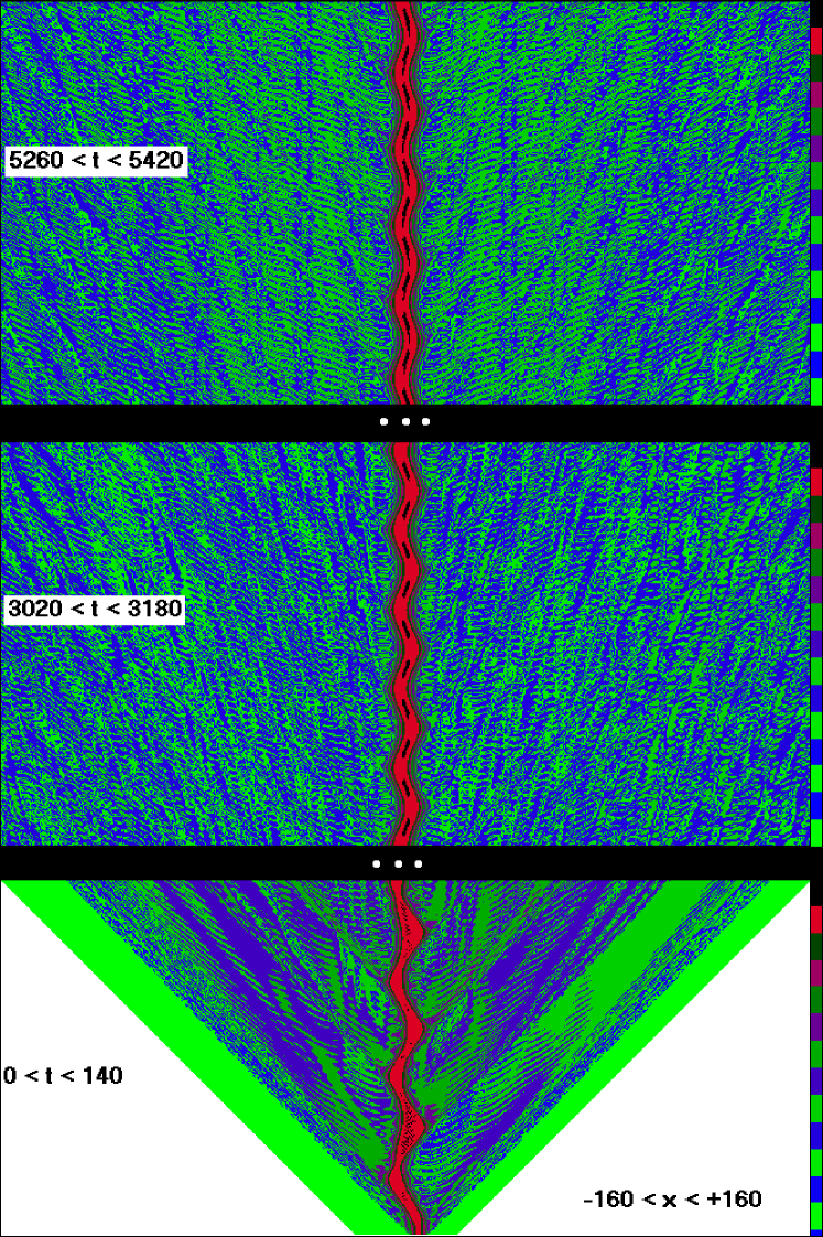
Figure 9: Adiabatic effective dynamics of solitons

Figure 9 represents a solution to equation (7.6) with the potential (7.4), where $a=10$, $m=6$ and $b=8.75$, $n=5$. We choose $V(x)=-0.2\cos(0.31x)$ and the initial conditions

$$\psi(x,0)=\phi_{\omega_{0}}(\gamma_{v_{0}}(x-q_{0})),\qquad\dot{\psi}(x,0)=0,$$ (7.9)

where $v_{0}=0$, $\omega_{0}=0.6$ and $q_{0}=5.0$. Note that the initial state does not belong to the solitary manifold. An effective width (half-amplitude) of the solitons is in the range $[4.4,5.6]$. It is quite small when compared with the spatial period of the potential $2\pi/0.31\sim 20$, which is confirmed by numerical simulations shown on Figure 9. Namely,
$\bullet$ Blue and green colors represent the dispersion wave with values $|\psi(x,t)|<0.01$, while the red color represents the soliton with values $|\psi(x,t)|\in[0.4,0.8]$.
$\bullet$ The soliton trajectory (‘red snake’) corresponds to oscillations of a classical particle in the potential $V(x)$.
$\bullet$ For $0<t<140$ the solution is rather distant from the solitary manifold, and the radiation is intense.
$\bullet$ For $3020<t<3180$ the solution approaches the solitary manifold, and the radiation weakens. The oscillation amplitude of the soliton is almost unchanged for a long time, confirming a Hamilton type dynamics.
$\bullet$ However, for $5260<t<5420$ the amplitude of the soliton oscillation is halved. This suggests that at a large time scale the deviation from the Hamilton effective dynamics becomes essential. Consequently, the effective dynamics gives a good approximation only on the adiabatic time scale $t\sim\varepsilon^{-1}$.
$\bullet$ The deviation from the Hamilton dynamics is due to radiation, which plays the role of dissipation.
$\bullet$ The radiation is realized as the dispersion waves which bring the energy to the infinity. The dispersion waves combine into uniformly moving bunches with discrete set of group velocities, as in Fig. 8. The magnitude of solutions is of order $\sim 1$ on the trajectory of the soliton, while the values of the dispersion waves is less than $0.01$ for $t>200$, so that their energy density does not exceed $0.0001$. The amplitude of the dispersion waves decays for large times.
$\bullet$ In the limit $t\to\pm\infty$ the soliton should converge to a static position corresponding to a local minimum of the potential. However, the numerical observation of this ”ultimate stage” is hopeless since the rate of the convergence decays with the decay of the radiation.

A Attractors and quantum postulates

The foregoing results on attractors of the nonlinear Hamilton equations were suggested by fundamental postulates of quantum theory, primarily Bohr’s postulate on transitions between quantum stationary orbits. Namely, in 1913 Bohr suggested ‘Columbus’s’ solution of the problem of stability of atoms and molecules [9], postulating that

Atoms and molecules are permanently on some stationary orbits $$|E_{m}\rangle E_{m}$$ with energies , and sometimes make transitions between the orbits,

$$|E_{m}\rangle\mapsto|E_{n}\rangle.$$ (A.1)

The simplest dynamic interpretation of this postulate is the attraction to stationary orbits (1.6) for any finite energy quantum trajectory $\psi(t)$. This means that the stationary orbits form a global attractor of the corresponding quantum dynamics.

However, this convergence contradicts the Schrödinger’s linear equation due to the superposition principle. Thus, Bohr’s transitions (A.1) in the linear theory do not exist.

It is natural to suggest that the attraction (1.6) holds for a nonlinear modification of the linear Schrödinger theory. Namely it turns out that the original Schrödinger theory is nonlinear, because it involves interaction with the Maxwell field. The corresponding nonlinear Maxwell–Schrödinger system is contained essentially in the first Schrödinger’s article of 1926:

$$\left\{\begin{aligned} &i\dot{\psi}(x,t)=\displaystyle\frac{1}{2}[-i\nabla+{\bf A}(x,t)+{\bf A}^{\rm ext}(x,t)]^{2}\psi(x,t)+[A_{0}(x,t)+A_{0}^{\rm ext}(x)]\psi(x,t)\\ &\Box A_{\alpha}(x,t)=4\pi J_{\alpha}(x,t),\qquad\alpha=0,1,2,3\end{aligned}\right|\quad x\in\mathbb{R}^{3},$$ (A.2)

where the units are chosen so that $\hbar=e=m=c=1$. Maxwell’s equations are written here in the 4-dimensional form, where $A=(A_{0},{\bf A})=(A_{0},A_{1},A_{2},A_{3})$ denotes the 4-dimensional potential of the Maxwell field with the Lorentz gauge $\dot{A}_{0}+\nabla\cdot{\bf A}=0$, $A^{\rm ext}=(A_{0}^{\rm ext},{\bf A}^{\rm ext})$ is an external 4-potential, and $J=(\rho,j_{1},j_{2},j_{3})$ is the 4-dimensional current. To make these equations a closed system, we must also express the density of charges and currents via the wave function:

$$J_{0}(x,t)=|\psi(x,t)|^{2};\qquad J_{k}(x,t)=[(-i\nabla_{k}+A_{k}(x,t)+A_{k}^{\rm ext}(x,t))\psi(x,t)]\cdot\psi(x,t),\quad k=1,2,3;$$ (A.3)

here ‘$\,\cdot\,$’ denotes the scalar product of two-dimensional real vectors corresponding to complex numbers. In particular, these expressions satisfy the continuity equation $\dot{\rho}+{\rm div~{}}j=0$ for any solution of the Schrödinger equation with arbitrary potentials [10, Section 3.4].

System (A.2) is non-linear in $(\psi,A)$ although the Schrödinger equation is formally linear in $\psi$. Now the question arises: what should be the stationary orbits for the nonlinear hyperbolic system (A.2)? It is natural to suggest that these are the solutions of type

$$(\psi(x)e^{-i\omega t},~{}A(x)).$$ (A.4)

Indeed, such functions give stationary distributions of charges and currents (A.3). Moreover, these functions are the trajectories of one-parameter subgroups of the symmetry group $U(1)$ of the system (A.2). Namely, for any solution $(\psi(x,t),A(x,t))$ and $\theta\in{\mathbb{R}}$ the functions

$$U_{\theta}(\psi(x,t),~{}A(x,t)):=(\psi(x,t)e^{i\theta},~{}A(x,t))$$ (A.5)

are also solutions. The same remarks apply to the Maxwell–Dirac system introduced by Dirac in 1927:

$$\left\{\begin{aligned} &\sum_{\alpha=0}^{3}\gamma^{\alpha}[i\displaystyle\nabla_{\alpha}-A_{\alpha}(x,t)-A_{\alpha}^{\rm ext}(x,t)]\psi(x,t)=m\psi(x,t)\\ &\Box\,A_{\alpha}(x,t)=J_{\alpha}(x,t):=\overline{\psi(x,t)}\gamma^{0}\gamma_{\alpha}\psi(x,t),\quad\alpha=0,\dotsc,3\ \ \end{aligned}\right|\quad x\in\mathbb{R}^{3},$$ (A.6)

where $\nabla_{0}:=\partial_{t}$. Thus, Bohr’s transitions (A.1) for the systems (A.2) and (A.6) with a static external potential $A^{\rm ext}(x,t)=A^{\rm ext}(x)$ can be interpreted as the long-time asymptotics

$$(\psi(x,t),~{}A(x,t))\sim(\psi_{\pm}(x)e^{-i\omega_{\pm}t},~{}A_{\pm}(x,t)),\qquad t\to\pm\infty$$ (A.7)

for every finite energy solution, where the asymptotics hold in a local norm. Obviously, the maps $U_{\theta}$ form the group isomorphic to $U(1)$, and the functions (A.4) are the trajectories of its one-parametric subgroups. Hence, the asymptotics (A.7) correspond to our general conjecture (1.4) with the symmetry group $U(1)$.

Furthermore, in the case of zero external potentials these systems are translation-invariant. Respectively, for their solutions one should expect the soliton asymptotics of type (1.10)

$$(\psi(x,t),A(x,t))\sim\displaystyle\sum\limits_{k}(\psi_{\pm}^{k}(x-v^{k}_{\pm}t)e^{i\Phi_{\pm}^{k}(x,t)},~{}A_{\pm}^{k}(x-v^{k}_{\pm}t))+(\varphi_{\pm}(x,t),~{}A_{\pm}(x,t)),\qquad t\to\pm\infty,$$ (A.8)

where the asymptotics hold in a global norm. Here $\Phi_{\pm}^{k}(x,t)$ are suitable phase functions, and each term-soliton is a solution to the corresponding nonlinear system, while $\varphi_{\pm}(x,t)$ and $A_{\pm}(x,t)$ represent some dispersion waves which are solutions to the free Schrödinger and Maxwell equations respectively. The existence of the solitons for the Maxwell-Dirac system is established in [35].

The asymptotics (A.7) and (A.8) are not proved yet for the Maxwell-Schrödinger and Maxwell-Dirac equations (A.2) and (A.6). One could expect that these asymptotics should follow by suitable modification of the arguments from Section 3. Namely, let the time spectrum of an omega-limit trajectory $\psi(x,t)$ contain at least two different frequencies $\omega_{1}\neq\omega_{2}$: for example, $\psi(x,t)=\psi_{1}(x)e^{-i\omega_{1}t}+\psi_{2}(x)e^{-i\omega_{2}t}$. Then the currents $J_{\alpha}(x,t)$ in the systems (A.2) and (A.6) contains the terms with the harmonics $e^{-i\Delta t}$ and $e^{i\Delta t}$, where $\Delta:=\omega_{1}-\omega_{2}\neq 0$. Thus the nonlinearity inflates the spectrum as in $U(1)$-invariant equations, considered in Section 3.

Further, these time-dependent harmonics on the right hand side of the Maxwell equations induce the radiation of an electromagnetic wave with the frequency $\Delta$ according to the limiting amplitude principle (3.62) since the continuous spectrum of the Maxwell generator is the whole line ${\mathbb{R}}$. Finally, this radiation brings the energy to infinity which is impossible for omega-limit trajectories. This contradiction suggests the validity of the one-frequency asymptotics (A.7). Let us note that the spectrum of the radiation contains the difference $\omega_{1}-\omega_{2}$ in accordance with the second Bohr postulate.

We have justified similar arguments rigorously for $U(1)$-invariant equations (3.1) and (3.13)–(3.15). However, for the systems (A.2) and (A.6) the rigorous justification is still an open problem.

References

- [1]
- [2]
- [3] L. Landau, On the problem of turbulence, C. R. (Doklady) Acad. Sci. URSS (N.S.) 44 (1944), 311–314. Attractors of dissipative PDEs
- [4] C. Foias, O. Manley, R. Rosa, R. Temam, Navier–Stokes Equations and Turbulence, Cambridge University Press, Cambridge, 2001.
- [5] J.K. Hale, Asymptotic Behavior of Dissipative Systems, American Mathematical Society, Providence, RI, 1988.
- [6] D. Henry, Geometric Theory of Semilinear Parabolic Equations, Lecture Notes in Mathematics, 840. Springer, Berlin–New York, 1981.
- [7] A.V. Babin, M.I. Vishik, Attractors of Evolution Equations, North–Holland Publishing Co., Amsterdam, 1992.
- [8] V.V. Chepyzhov, M.I. Vishik, Attractors for Equations of Mathematical Physics, American Mathematical Society, Providence, RI, 2002. Quantum theory
- [9] N. Bohr, Phil. Mag. 26 (1913) 1-25; 476-502; 857-875. http://www.nba.nbi.dk/pdffiles/trilogy.pdf
- [10] A. Komech, Quantum Mechanics: Genesis and Achievements, Springer, Dordrecht, 2013.
- [11] J.J. Sakurai, Advanced Quantum Mechanics, Addison-Wesley, Reading Massachusetts, 1967.
- [12] W. Heisenberg, Der derzeitige Stand der nichtlinearen Spinortheorie der Elementarteilchen, Acta Phys. Austriaca 14 (1961), 328–339.
- [13] W. Heisenberg, Introduction to the Unified Field Theory of Elementary Particles, Interscience, London, 1966.
- [14] F. Bonetto, J.L. Lebowitz, L. Rey-Bellet, Fourier’s law: a challenge to theorists, pp. 128–150 in: Fokas, A. (ed.) et al., Mathematical Physics 2000. International Congress, London, GB, 2000. London: Imperial College Press, 2000.
- [15] M. Gell-Mann,Symmetries of baryons and mesons, Phys. Rev. (2) 125 (1962), 1067–1084.
- [16] Y. Ne’eman, Unified interactions in the unitary gauge theory, Nuclear Phys. 30 (1962), 347–349.
- [17] R.K. Adair, E.C. Fowler, Strange Particles, Interscience Publ., New York, 1963.
- [18] F. Halzen, A. Martin, Quarks & Leptons: An Introductory Course in Modern Particle Physics, John Wiley & Sons, 1984.
- [19] V.E. Barnes & al, Observation of a hyperon with strangeness minus three, Phys. Rev. Letters 12 (1964), no. 8, 204–206. General theory of nonlinear PDEs
- [20] E. Hopf, Über die Anfangswertaufgabe für die hydrodynamischen Grundgleichungen, Math. Nachr. 4 (1951), 213–231.
- [21] K. Jörgens, Das Anfangswertproblem im Grossen für eine Klasse nichtlinearer Wellengleichungen, Math. Z. 77 (1961), 295–308.
- [22] J.-L. Lions, Quelques Méthodes de Résolution des Problèmes aux Limites non Linéaires, Dunod; Gauthier-Villars, Paris, 1969. Local energy decay
- [23] I. Segal, Quantization and dispersion for nonlinear relativistic equations, Proc. Conf. Mathematical Theory of Elementary Particles (Dedham, Mass., 1965), M.I.T. Press, Cambridge, Mass., 1966, pp. 79–108.
- [24] I. Segal, Dispersion for non-linear relativistic equations. II, Ann. Sci. Sc. Norm. Sup. (4) 1 (1968), 459–497.
- [25] C. S. Morawetz, Time decay for the nonlinear Klein–Gordon equation, Proc. Roy. Soc. Ser. A 306 (1968), 291–296.
- [26] W. A. Strauss, Decay and asymptotics for , J. Functional Analysis 2 (1968), 409–457.
- [27] C.S. Morawetz, W.A. Strauss, Decay and scattering of solutions of a nonlinear relativistic wave equation, Comm. Pure Appl. Math. 25 (1972), 1–31.
- [28] W.A. Strauss, Nonlinear scattering theory at low energy, J. Funct. Anal. 41 (1981), no. 1, 110–133.
- [29] W.A. Strauss, Nonlinear scattering theory at low energy: sequel, J. Funct. Anal. 43 (1981), no. 3, 281–293. Existence of stationary orbits and solitons
- [30] W.A. Strauss, Existence of solitary waves in higher dimensions, Comm. Math. Phys. 55 (1977), 149–162.
- [31] H. Berestycki, P.-L. Lions, Nonlinear scalar field equations. I. Existence of a ground state, Arch. Rational Mech. Anal. 82 (1983), no. 4, 313–345.
- [32] H. Berestycki, P.-L. Lions, Nonlinear scalar field equations. II. Existence of infinitely many solutions, Arch. Rational Mech. Anal. 82 (1983), no. 4, 347–375.
- [33] L. Lusternik, L. Shnirelmann, Méthodes Topologiques dans les Problèmes Variationels, Hermann, Paris, 1934.
- [34] L. Lusternik, L. Shnirelmann, Topological methods in variational problems and their applications to differetial geometry of surfaces, Uspekhi Matem. Nauk, 2:1(17) (1947), 166–217 [in Russian].
- [35] M.J. Esteban, V. Georgiev, E. Séré, Stationary solutions of the Maxwell–Dirac and the Klein–Gordon–Dirac equations, Calc. Var. Partial Differential Equations 4 (1996), no. 3, 265–281. Orbital stability of solitary waves
- [36] M. Grillakis, J. Shatah, W. Strauss, Stability theory of solitary waves in the presence of symmetry. I. J. Funct. Anal. 74 (1987), no. 1, 160–197.
- [37] M. Grillakis, J. Shatah, W. Strauss, Stability theory of solitary waves in the presence of symmetry. II. J. Funct. Anal. 94 (1990), no. 2, 308–348. Global attraction to stationary states
- [38] H. Lamb, On a peculiarity of the wave-system due to the free vibrations of a nucleus in an extended medium, Proc. London Math. Soc. 32 (1900), 208–211.
- [39] A. Komech, On the stabilization of interaction of a string with a nonlinear oscillator, Moscow Univ. Math. Bull. 46 (1991), no. 6, 34–39.
- [40] A. Komech, On stabilization of string-nonlinear oscillator interaction, J. Math. Anal. Appl. 196 (1995), 384–409.
- [41] A. Komech, On the stabilization of string-oscillators interaction, Russian Journal of Mathematical Physics 3 (1995), 227–248.
- [42] A. Komech, On transitions to stationary states in one-dimensional nonlinear wave equations, Arch. Rat. Mech. Anal. 149 (1999), no. 3, 213–228.
- [43] A. Komech, Attractors of nonlinear Hamiltonian one-dimensional wave equations, Russian Math. Surveys 55 (2000), no. 1, 43–92. (Translation from Uspekhi Mat. Nauk 55 (2000), no. 1(331), 45–98. [Russian])
- [44] A. Komech, H. Spohn, M. Kunze, Long-time asymptotics for a classical particle interacting with a scalar wave field, Comm. Partial Diff. Equs. 22 (1997), no.1/2, 307–335.
- [45] A.Komech, H.Spohn, Long-time asymptotics for the coupled Maxwell–Lorentz equations, Comm. Partial Diff. Equs. 25 (2000), no.3/4, 558–585.
- [46] J.D. Jackson, Classical Electrodynamics, 3-rd edition, N.-Y., Wiley, 1999.
- [47] H. Spohn, Dynamics of Charged Particles and their Radiation Field, Cambridge University Press, Cambridge, 2004.
- [48] A.I. Komech, A.E. Merzon, Scattering in the nonlinear Lamb system, Physics Letters A 373 (2009), 1005–1010.
- [49] A.I. Komech, A.E. Merzon, On asymptotic completeness of scattering in the nonlinear Lamb system, J. Math. Physics 50 (2009), 023514-1–023514-10.
- [50] A.I. Komech, A.E. Merzon, On asymptotic completeness of scattering in the nonlinear Lamb system II, J. Math. Physics 54(2013), 012702–012710. arXiv:1205.5850 Asymptotic stability of stationary orbits
- [51] M.I. Weinstein, Modulational stability of ground states of nonlinear Schrödinger equations, SIAM Journal on Mathematical Analysis 16, no. 3, 472–491.
- [52] A. Soffer, M.I. Weinstein, Multichannel nonlinear scattering in nonintegrable systems, Commun. Math. Phys 133 (1990), 119–146.
- [53] A. Soffer, M.I. Weinstein, Multichannel nonlinear scattering and stability II. The case of Anisotropic and potential and data, J. Differential Equations 98 (1992), 376–390.
- [54] C.-A. Pillet, C.E. Wayne, Invariant manifolds for a class of dispersive, Hamiltonian, partial differential equations, J. Differential Equations 141 (1997), no. 2, 310–326.
- [55] A. Soffer, M.I. Weinstein, Resonances, radiation damping and instability in Hamiltonian nonlinear wave equations, Invent. Math. 136 (1999), no. 1, 9–74.
- [56] A. Soffer, M.I. Weinstein, Selection of the ground state for nonlinear Schrödinger equations, Reviews in Mathematical Physics 16 (2004) no. 8, 977–1071.
- [57] A. Soffer, Soliton dynamics and scattering, 459–471, in: International Congress of Mathematicians, Vol. III, Eur. Math. Soc., Zürich, 2006.
- [58] T.-P. Tsai, H.-T. Yau, Classification of asymptotic profiles for nonlinear Schrödinger equations with small initial data, Adv. Theor. Math. Phys. 6 (2002), no. 1, 107–139.
- [59] T.-P. Tsai, H.-T. Yau, Asymptotic dynamics of nonlinear Schrödinger equations: resonance-dominated and dispersion-dominated solutions, Comm. Pure Appl. Math. 55 (2002), 153–216.
- [60] T.-P. Tsai, Asymptotic dynamics of nonlinear Schrödinger equations with many bound states, J. Differential Equations 192 (2003), 225–282.
- [61] V. Buslaev, A. Komech, E. Kopylova, D. Stuart, On asymptotic stability of solitary waves Comm. Partial Diff. Eqns 33 (2008), no. 4, 669–705. arXiv:math-ph/0702013
- [62] A. Komech, E. Kopylova, D. Stuart, On asymptotic stability of solitary waves for Schödinger equation coupled to nonlinear oscillator II, Comm. Pure Appl. Anal. 202 (2012), no. 3, 1063–1079. arXiv:0807.1878 Asymptotic stability of solitons
- [63] V.S. Buslaev, G.S. Perelman, Scattering for the nonlinear Schrödinger equation: states close to a soliton, St. Petersburg Math. J.4 (1993), 1111–1142.
- [64] V.S. Buslaev, G.S. Perelman, On the stability of solitary waves for nonlinear Schrödinger equations, Amer. Math. Soc. Trans. (2) 164 (1995), 75–98.
- [65] V.S. Buslaev, C. Sulem, On asymptotic stability of solitary waves for nonlinear Schrödinger equations, Ann. Inst. Henri Poincaré, Anal. Non Linéaire 20 (2003), no.3, 419–475.
- [66] R. Pego, M. I. Weinstein, Asymptotic stability of solitary waves. Comm. Math. Phys. 164 (1994), 305–349.
- [67] J. Miller and M. Weinstein, Asymptotic stability of solitary waves for the regularized long-wave equation. Comm. Pure Appl. Math. 49 (1996), 399–441.
- [68] S. Cuccagna, Stabilization of solutions to nonlinear Schrödinger equations, Comm. Pure Appl. Math. 54 (2001), no. 9, 1110–1145.
- [69] Y. Martel, F. Merle, Asymptotic stability of solitons of the subcritical gKdV equations revisited, Nonlinearity 18 (2005), no. 1, 55–80.
- [70] H. Lindblad, T. Tao, Asymptotic decay for a one-dimensional nonlinear wave equation, Anal. PDE 5 (2012), no. 2, 411–422.
- [71] V. Imaykin, A. Komech, B. Vainberg, On scattering of solitons for the Klein–Gordon equation coupled to a particle, Comm. Math. Phys. 268 (2006), no. 2, 321–367. arXiv:math.AP/0609205
- [72] V. Imaykin, A. Komech, H. Spohn, Scattering asymptotics for a charged particle coupled to the Maxwell field, J. Math. Physics 52 (2011), no. 4, 042701-1–042701-33. arXiv:0807.1972
- [73] A. Komech, E. Kopylova, Scattering of solitons for Schrödinger equation coupled to a particle, Russian J. Math. Phys. 13 (2006), no. 2, 158–187. arXiv:math.AP/0609649
- [74] A. Komech, E. Kopylova, H. Spohn, Scattering of solitons for Dirac equation coupled to a particle, J. Math. Analysis and Appl. 383 (2011), no. 2, 265–290. arXiv:1012.3109
- [75] V. Imaykin, A. Komech, B.Vainberg, Scattering of solitons for coupled wave-particle equations, J. Math. Analysis and Appl. 389 (2012), no. 2, 713–740. arXiv:1006.2618
- [76] V. Imaikin, Soliton asymptotics for systems of ‘field-particle’ type, Russian Math. Surveys 68 (2013), no. 2, 227–281. (Translation from Uspekhi Mat. Nauk 68 (2013), no. 2(410), 33–90. [Russian])
- [77] A. Bensoussan, C. Iliine, A. Komech, Breathers for a relativistic nonlinear wave equation, Arch. Rat. Mech. Anal. 165 (2002), 317-345.
- [78] E. Kopylova, A. Komech, On asymptotic stability of moving kink for relativistic Ginzburg–Landau equation, Comm. Math. Physics 302 (2011), no. 1, 225–252. ArXiv:0910.5538
- [79] E. Kopylova, A. Komech, On asymptotic stability of kink for relativistic Ginzburg–Landau equation, Arch. Rat. Mech. Anal. 202 (2011), no. 2, 213–245. ArXiv:0910.5539
- [80] E. Kopylova, Asymptotic stability of solitons for nonlinear hyperbolic equations, Russian Math. Surveys 68 (2013), no. 2, 283–334. (Translation from Uspekhi Mat. Nauk 68 (2013), no. 2(410), 91–144. [Russian])
- [81] A.I. Komech, E.A. Kopylova, S.A. Kopylov, On nonlinear wave equations with parabolic potentials, J. Spec. Theory 3 (2013), no. 4, 485–503. arXiv:1206.6073
- [82] A. Komech, E. Kopylova, On eigenfunction expansion of solutions to the Hamilton equations, J. Stat. Phys. 154 (2014), no. 1-2, 503–521. arXiv:1308.0485.
- [83] N. Boussaid, S. Cuccagna, On stability of standing waves of nonlinear Dirac equations, Comm. Partial Differential Equations 37 (2012), no. 6, 1001–1056.
- [84] J. Fröhlich, Z. Gang, Emission of Cherenkov radiation as a mechanism for Hamiltonian friction, Advances in Mathematics 264 (2014), 183–235
- [85] Y. Martel, F. Merle, T.-P. Tsai, Stability and asymptotic stability in the energy space of the sum of N solitons for subcritical gKdV equations, Comm. Math. Phys. 231 (2002), no. 2, 347–373.
- [86] G. Perelman, Asymptotic stability of multi-soliton solutions for nonlinear Schrödinger equations, Comm. Partial Differential Equations 29 (2004), no. 7–8, 1051–1095.
- [87] I. Rodnianski, W. Schlag, A. Soffer, Asymptotic stability of N-soliton states of NLS. Arxiv preprint math.AP/0309114 (2003)
- [88] I. Rodnianski, W. Schlag, A. Soffer, Dispersive analysis of charge transfer models, Comm. Pure Appl. Math. 58 (2005), no. 2, 149–216.
- [89] M. Reed, B. Simon, Methods of Modern Mathematical Physics. Analysis of Operators, Vol. IV, Academic Press, New York, 1978.
- [90] I.M. Sigal, Nonlinear wave and Schrödinger equations. I: Instability of periodic and quasiperiodic solutions. Commun. Math. Phys. 153 (1993), no. 2, 297 320.
- [91] M. Merkli, I.M. Sigal, A time-dependent theory of quantum resonances. Commun. Math. Phys. 201 (1999), no. 3, 549 576. Dispersion decay
- [92] S. Agmon, Spectral properties of Schrödinger operator and scattering theory, Ann. Scuola Norm. Sup. Pisa, Ser. IV 2 (1975), 151–218.
- [93] A. Jensen, T. Kato, Spectral properties of Schrödinger operators and time-decay of the wave functions, Duke Math. J. 46 (1979), 583–611.
- [94] E. Kopylova, A. Komech, Dispersion Decay and Scattering Theory, John Wiley & Sons, Hoboken, NJ, 2012.
- [95] E. Kopylova, Dispersion estimates for the Schrödinger and Klein–Gordon equations, Russian Math. Surveys 65 (2010), no. 1, 95–142. (Translation from Uspekhi Mat. Nauk 65 (2010), no. 1(391), 97–144. [Russian])
- [96] A. Komech, E. Kopylova, Weighted decay for magnetic Schrödinger equation, J. Funct. Analysis 264 (2013), no. 3, 735–751.
- [97] A. Komech, E. Kopylova, M. Kunze, Dispersion estimates for 1D discrete Schrödinger and Klein–Gordon equations, Applicable Analysis 85 (2006), no. 12, 1487–1508.
- [98] A. Komech, E. Kopylova, B. Vainberg, On dispersion properties of discrete 2D Schrödinger and Klein–Gordon equations, J. Funct. Anal. 254 (2008), no. 8, 2227–2254.
- [99] E. Kopylova, On dispersion estimates for discrete 3D Schrödinger and Klein–Gordon equation, St. Petersburg Math. J. 21 (2010), 743–760. ArXiv 0812.0468. Global attraction to stationary orbits
- [100] A.I. Komech, On attractor of a singular nonlinear -invariant Klein–Gordon equation, p. 599–611 in: Proc. ISAAC Congress, Berlin, 2003.
- [101] A.I. Komech, A.A. Komech, On global attraction to solitary waves for the Klein–Gordon equation coupled to nonlinear oscillator, C. R., Math., Acad. Sci. Paris 343, Issue 2, 15 July 2006, Pages 111–114.
- [102] A.I. Komech, A.A. Komech, Global attractor for a nonlinear oscillator coupled to the Klein–Gordon field, Arch. Rat. Mech. Anal. 185 (2007), 105–142.
- [103] A.I. Komech, A.A. Komech, On global attraction to solitary waves for the Klein–Gordon field coupled to several nonlinear oscillators, J. Math. Pures App., 93 (2010), 91–111. arXiv:math/0702660
- [104] A.I. Komech, A.A. Komech, Global Attraction to Solitary Waves in Models Based on the Klein–Gordon Equation SIGMA, Symmetry Integrability Geom. Methods Appl. 4, Paper 010, 23 pages, electronic only (2008). http://www.emis.de/journals/SIGMA/2008/arXiv:math-ph/0711.0041
- [105] A.I. Komech, A.A. Komech, Global attraction to solitary waves for Klein–Gordon equation with mean field interaction, Annales de l’IHP-ANL 26 (2009), no. 3, 855–868. arXiv:math-ph/0711.1131
- [106] A.I. Komech, A.A. Komech, Global attraction to solitary waves for nonlinear Dirac equation with mean field interaction, SIAM J. Math. Analysis, 42 (2010), no. 6, 2944–2964. arXiv:0910.0517, http://link.aip.org/link/?SJM/42/2944
- [107] A. Comech, Weak attractor of the Klein–Gordon field in discrete space-time interacting with a nonlinear oscillator, Discrete Contin. Dyn. Syst. 33 (2013), no. 7, 2711–2755.
- [108] A.A. Komech, A.I. Komech, A variant of the Titchmarsh convolution theorem for distributions on the circle, Funct. Anal. Appl. 47 (2013), no. 1, 21–26. (Translation from Funktsional. Anal. i Prilozhen. 47 (2013), no. 1, 26–32. [Russian])
- [109] A.I. Komech, Linear Partial Differential Equations with Constant Coefficients, pp. 125–255 in: Yu.V. Egorov, A.I. Komech, M.A. Shubin, Elements of the Modern Theory of Partial Differential Equations, Springer, Berlin, 1999.
- [110] G. Gaudry, Quasimeasures and operators commuting with convolution, Pacific J. Math. 18 (1966), 461–476.
- [111] E. Titchmarsh, The zeros of certain integral functions, Proc. of the London Math. Soc. 25 (1926), 283–302.
- [112] B.Y. Levin, Lectures on Entire Functions, American Mathematical Society, Providence, RI, 1996, in collaboration with and with a preface by Yu. Lyubarskii, M. Sodin and V. Tkachenko.
- [113] L. Hörmander, The Analysis of Linear Partial Differential Operators. I, Springer Study Edition, Springer, Berlin, 1990.
- [114] O. A. Ladyzhenskaya, On the principle of limit amplitude. [Russian] Uspehi Mat. Nauk (N.S.) 12 (1957), no. 3(75), 161–164.
- [115] C. S. Morawetz, The limiting amplitude principle, Comm. Pure Appl. Math. 15 (1962), 349–361.
- [116] L. Lewin, Advanced Theory of Waveguides, Iliffe and Sons, Ltd., London, 1951. Global attraction to solitons
- [117] W. Eckhaus, A. van Harten, The Inverse Scattering Transformation and the Theory of Solitons, Elsevier, North–Holland, 1981.
- [118] A. Komech, H. Spohn, Soliton-like asymptotics for a classical particle interacting with a scalar wave field, Nonlinear Analysis 33 (1998), no.1, 13–24.
- [119] V. Imaikin, A. Komech, N. Mauser, Soliton-type asymptotics for the coupled Maxwell–Lorentz equations, Ann. Inst. Poincaré, Phys. Theor. 5 (2004), 1117–1135.
- [120] V. Imaikin, A.Komech, H. Spohn, Scattering theory for a particle coupled to a scalar field, Journal of Discrete and Continuous Dynamical Systems 10 (2004), no. 1&2, 387–396.
- [121] V. Imaikin, A.Komech, P. Markowich, Scattering of solitons of the Klein–Gordon equation coupled to a classical particle, Journal of Mathematical Physics 44 (2003), no. 3, 1202–1217.
- [122] V. Imaikin, A. Komech, H. Spohn, Soliton-like asymptotics and scattering for a particle coupled to Maxwell field, Russian Journal of Mathematical Physics 9 (2002), no. 4, 428–436.
- [123] V. Imaikin, A.Komech, H. Spohn, Rotating charge coupled to the Maxwell field: scattering theory and adiabatic limit, Monatshefte fuer Mathematik 142 (2004), no. 1–2, 143–156.
- [124] A. Komech, N. Mauser, A. Vinnichenko, On attraction to solitons in relativistic nonlinear wave equations, Russ. J. Math. Phys. 11 (2004), no. 3, 289–307.
- [125] T. Dudnikova, A. Komech, H. Spohn, Energy-momentum relation for solitary waves of relativistic wave equation, Russian Journal Math. Phys. 9 (2002), no. 2, 153–160.
- [126] G.L. Lamb, Elements of Soliton Theory, Wiley, New-York, 1980 Adiabatic effective dynamics of solilons
- [127] M. Abraham, Dynamik des Elektrons, Physikal. Zeitschr. 4 (1902), 57–63; Gött. Nachr. 20–41 (1902).
- [128] M. Abraham, Theorie der Elektrizität, Bd.2: Elektromagnetische Theorie der Strahlung, Teubner, Leipzig, 1905.
- [129] A. Einstein, Ist die Trägheit eines Körpers von seinem Energieinhalt abhängig?, Annalen der Physik 18 (1905), no. 13, 639–643.
- [130] L. Houllevigue, L’Évolution des Sciences, A.Collin, Paris, 1908.
- [131] R.P. Feynman, R.B. Leighton, M. Sands, The Feynman Lectures on Physics. Vol. 2: Mainly Electromagnetism and Matter. Addison-Wesley Publishing Co., Inc., Reading, Mass.-London, 1964.
- [132] A. Komech, M.Kunze, H.Spohn, Effective Dynamics for a mechanical particle coupled to a wave field, Comm. Math. Phys. 203 (1999), 1–19.
- [133] M. Kunze, H. Spohn, Adiabatic limit for the Maxwell–Lorentz equations, Ann. Henri Poincaré 1 (2000), no. 4, 625–653.
- [134] J. Fröhlich, T.P. Tsai, H.T. Yau, On the point-particle (Newtonian) limit of the non-linear Hartree equation, Comm. Math. Physics 225 (2002), no.2, 223–274.
- [135] J. Fröhlich, S. Gustafson, B.L.G. Jonsson, I.M. Sigal, Solitary wave dynamics in an external potential, Comm. Math. Phys. 250 (2004), no. 3, 613–642.
- [136] D. Stuart, Existence and Newtonian limit of nonlinear bound states in the Einstein–Dirac system. J. Math. Phys. 51 (2010), no. 3, 032501–032513. arXiv:0906.4661
- [137] S. Demoulini, D. Stuart Adiabatic limit and the slow motion of vortices in a Chern–Simons–Schrödinger system. Comm. Math. Phys. 290 (2009), no. 2, 597–632. arXiv:0905.0998
- [138] E. Long, D. Stuart, Effective dynamics for solitons in the nonlinear Klein–Gordon–Maxwell system and the Lorentz force law, Rev. Math. Phys. 21 (2009), no. 4, 459–510. arXiv:0905.0982
- [139] V. Bach, T. Chen, J. Faupin, J. Fröhlich, I.M. Sigal, Effective dynamics of an electron coupled to an external potential in non-relativistic QED, Ann. Henri Poincaré 14 (2013), no. 6, 1573–1597.