Improving Efficiency and Scalability of
Formula-based Debugging

Abstract

Formula-based debugging techniques are becoming increasingly popular, as they provide a principled way to identify potentially faulty statements together with information that can help fix such statements. Although effective, these approaches are computationally expensive, which limits their practical applicability. Moreover, they tend to focus on failing test cases alone, thus ignoring the wealth of information provided by passing tests. To mitigate these issues, we propose two techniques: on-demand formula computation (OFC) and clause weighting (CW). OFC improves the overall efficiency of formula-based debugging by exploring all and only the parts of a program that are relevant to a failure. CW improves the accuracy of formula-based debugging by leveraging statistical fault-localization information that accounts for passing tests. Our empirical results show that both techniques are effective and can improve the state of the art in formula-based debugging.

I Introduction

Because debugging is expensive and time consuming, there has been a great deal of research on automated techniques for supporting various debugging tasks (e.g., [39, 25, 28, 29, 6, 34, 30, 9, 40, 10]). Recently, in particular, there has been a considerable interest in techniques that can perform fault localization in a more principled way (e.g., [26, 36, 20, 14]). These techniques, collectively called formula-based debugging, model faulty programs and failing executions as formulas and perform fault localization by manipulating and solving these formulas. As a result, they can provide developers with the possible location of the fault, together with a mathematical explanation of the failure (e.g., the fact that an expression should have produced a different value or that a different branch should have been taken at a conditional statement).

BugAssist [26] is a technique of particular interest in this arena. Given a faulty program, a failing input, and a corresponding (violated) assertion, BugAssist performs fault localization by constructing an unsatisfiable Boolean formula that encodes (1) the input values, (2) the semantics of (a bounded version of) the faulty program, and (3) the assertion. It then uses a pMAX-SAT solver to find maximal sets of clauses in this formula that can be satisfied together and outputs the complement sets of clauses (CoMSS) as potential causes of the error. Intuitively, each set of clauses in CoMSS indicates a corresponding set of statements that, if suitably modified (e.g., replacing the statements with angelic values [12]), would make the program behave correctly for the considered input.

Although effective, BugAssist is extremely computationally expensive, as it builds a formula for (a bounded unrolling of) all possible paths in a program. This can lead to formulas with millions of terms [26] and scalability issues even for small programs. Moreover, BugAssist, like most formula-based debugging approaches, does not take into account passing test cases, thus missing two important opportunities. First, passing executions can help identify statements, and thus parts of the formulas, that are less likely to be related to the fault, which can help optimizing the search for a solution to such formulas. Second, passing executions can help filtering out locations that may be potential fixes for the failing executions considered but could break previously passing test cases if modified [12].

In this paper, we propose two possible ways of addressing these issues and improving formula-based debugging approaches: on-demand formula computation (OFC) and clause weighting (CW). OFC is a novel on-demand algorithm that can dramatically reduce the number of paths encoded in a formula, and thus the overall complexity of such formula and the cost of computing a pMAX-SAT solution for it. Intuitively, our algorithm (1) builds a formula for the path in the original failing trace, (2) analyzes the formula to identify additional relevant paths to consider, (3) expands the formula by encoding these additional paths, (4) repeats (2) and (3) until no more relevant paths can be identified, at which point it (5) reports the computed solution. CW accounts for the information provided by passing test cases by assign weights to the different clauses in an encoded formula based on the suspiciousness values computed by a statistical fault localization technique. Doing so has the potential to improve the accuracy of the results by helping the solver compute CoMSSs that are more likely to correspond to faulty statements. (The guidance provided to the solver can also unintentionally improve the efficiency of the approach, as we show in Section IV-B1.) To assess the effectiveness of OFC and CW, we selected BugAssist as a baseline and considered four different formula-based debugging techniques: the original BugAssist, BugAssist+CW, OFC, and OFC+CW. We implemented all four techniques in a tool that works on C programs and used the tool to perform an empirical study. In the study, we first applied the four techniques to $52$ versions of two small programs to assess several tradeoffs involved in the use of CW and OFC and compare with related work. Our results are encouraging, as they show that CW and OFC can improve the performance of BugAssist in several respects. First, the use of CW resulted in more accurate results—in terms of position of the actual fault in the ranked list of statements reported to developers—in the majority of the cases considered. Second, CW and OFC were able to reduce the computational cost of BugAssist by 27% and 75% on average, respectively, with maximum speedups of over 70X for OFC. Most importantly, our results show that these improvements, and especially OFC, allow formula-based debugging to handle faults that go beyond the capability of an all-paths analysis such as the one performed by BugAssist. To further demonstrate the practicality of CW and OFC, we also performed a case study on a real-world bug in Redis, a popular open source project. Overall, our results show that CW and OFC are promising steps towards more practically applicable formula-based debugging techniques and motivate further research in this direction.

The main contributions of this paper are:

• The definition of clause weighting and on-demand formula computation, two approaches for improving the accuracy and efficiency of formula-based debugging.

• A prototype implementation of our technique that is available for download, together with our experimental infrastructure and benchmark programs (see http://www.cc.gatech.edu/~orso/software/odin/).

• Initial empirical evidence that CW and OFC are as effective, more efficient, and potentially more practically applicable than existing approaches.

II Background

SSA Form

Given a program $P$, the static single assignment (SSA) form of $P$ is a program semantically equivalent to $P$ in which each variable is assigned exactly once [17]. Because multiple definitions can reach a join point, for each conditional statement $cs$, the SSA form contains one $\phi$ function phi for each definition $d$ in the original program that is control dependent on $cs$ and can reach $cs$’s join point. phi is located at the join point and selects the correct definition to use at that point depending on which branch of $cs$ was executed. We refer to conditional statement $cs$ as phi’s conditional.

Statistical Fault Localization

Spectrum-based statistical fault localization techniques compute the correlation between a program entity and an observed failure based on how the entity was exercised in passing and failing executions (e.g., [25, 29, 5]). They use this correlation as an approximation of the likelihood of a program entity to be faulty. We leverage the Ochiai fault localization approach, which has shown to be quite effective in empirical comparisons [5].

MAX-SAT, pMAX-SAT, and wpMAX-SAT Problems

MAX-SAT is the problem of determining the maximum number of clauses of a given unsatisfiable Boolean formula that can be satisfied by some assignment [11]. An extension of MAX-SAT is pMAX-SAT, in which clauses are marked as either hard (i.e., clauses that cannot be dropped) or soft (i.e., clauses that can be dropped). wpMAX-SAT extends pMAX-SAT by assigning weights to soft clauses, such that clauses with higher weights are less likely to be dropped. A solution to a wpMAX-SAT problem is a maximal satisfiable subset of clauses (MSS) with maximum weight in which all hard clauses are satisfied. The complement of MSS is called CoMSS. MSS is defined as a maximal set of clauses, in the sense that adding any of the other clauses in CoMSS would make the set unsatisfiable. The maximal property of MSS and the minimal property of CoMSS essentially imply that clauses in CoMSS are responsible for making the formula unsatisfiable. There may be several different maximal satisfiable subsets and complementary sets for a given MAX-SAT problem, and each of these sets can contain multiple clauses.

III Improving Formula-based Debugging

As we discussed in the Introduction, the goal of this work is to investigate ways to mitigate some of the limitations of existing formula-based debugging approaches. To this end, we propose two approaches: clause weighting and on-demand formula computation. We discuss them in detail using BugAssist [26] as a representative of state-of-the-art formula-based debugging techniques and our baseline.

III-A Clause Weighting (CW)

CW consists of using the information from passing executions to inform a wpMAX-SAT solver. More precisely, CW leverages the suspiciousness values computed by a statistical fault localization technique and assigns to each program entity $en$, and thus to the corresponding clause in the program formula, a weight inversely proportional to its suspiciousness $susp(en)$: $weight(en)=1/susp(en)$. If the suspiciousness value of an entity is zero, which means that the entity is only executed by passing tests, CW assigns to it the largest possible weight. By assigning different weights to different clauses, CW transforms the original pMAX-SAT problem in BugAssit into a wpMAX-SAT problem. The rationale for CW is that, by the definition of wpMAX-SAT, clauses with higher weights are more likely to be included in an MSS (i.e., less likely to be identified as causes of the faulty behavior), while clauses with lower weights are less likely to be included in an MSS (i.e., more likely to be included in a CoMSS and thus be identified as causes of the faulty behavior).

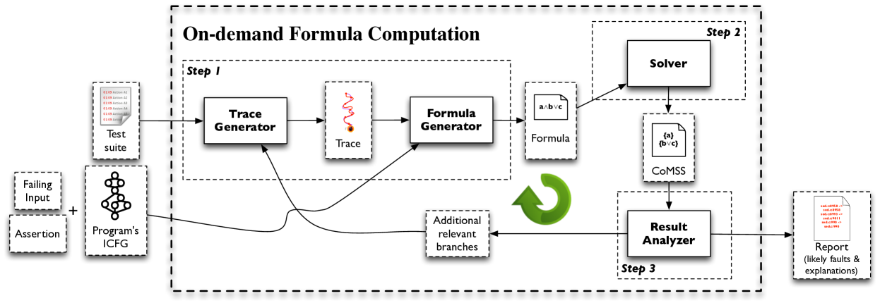
Figure 1: Overview of on-demand formula computation.

Formula-based debugging techniques such as BugAssist consider all possible pMAX-SAT solutions equally and simply report them. Conversely, by leveraging the heuristics in statistical fault localization, CW is more likely to rank the set of clauses corresponding to the fault at the top of the list of solutions, thus reducing developers’ debugging effort. This potential advantage, however, comes at a cost. Solving wpMAX-SAT problems can be computationally more expensive than solving a pMAX-SAT problem, which can outweigh CW’s benefits. To understand this tradeoff, in our empirical evaluation we assess how CW affects the accuracy and efficiency of formula-based debugging (see Section IV-B1).

III-B On-demand Formula Computation (OFC)

OFC is our second, and more substantial, improvement over traditional formula-based debugging techniques. Figure 1 shows an overall view of OFC and its workflow. The inputs to the algorithm are a faulty program, represented as an Inter-procedural Control Flow Graph (ICFG), and a test suite that contains a set of passing tests and one failing test. (We discuss how OFC could leverage the presence of multiple failing inputs in Section III-B6.) As it is common practice for debugging techniques, we assume that a failure can be expressed as the violation of an assertion in the program. Given these inputs, OFC produces as output a set of clauses and their corresponding program entities (i.e., branches and statements). These are entities that, if suitably modified, would make the failing execution pass. The expressions in the reported clauses provide developers with additional information on the failure, and can be considered a “mathematical explanation” of the failure.

As Figure 1 shows, OFC consists of three main steps. The key idea behind OFC is to reason about the failure (and the program) incrementally, by starting with the entities traversed in a single failing trace, computing CoMSS solutions for the partial program exercised by the trace, and then expanding the portion of the program considered in the analysis when such solutions indicate that additional control-flow paths should be taken into consideration to “explain” the failure. Specifically, in its first step (Section III-B1), OFC generates a new trace (the original failing trace, in the first iteration) and suitably updates the trace formula, a formula that encodes the semantics of the traces generated so far. OFC’s second step (Section III-B2) computes the CoMSSs of the (unsatisfiable) formula built in the previous step. Finally, in OFC’s third step, the algorithm checks whether there is any additional relevant branch to consider in the program (Section III-B3). If so, OFC returns to Step 1. Otherwise, it computes all possible CoMSSs of the final formula to report to developers the set of relevant clauses and their corresponding program entities.

Algorithm 1 shows the main algorithm, which takes as inputs the ICFG of the faulty program and the program’s test suite and performs the three steps we just described. We discuss each step in detail in the rest of this section.

III-B1 Trace Generator and Formula Generator

After an initialization phase, OFC iterates Steps 1, 2, and 3. Step 1 performs two tasks: trace generation and formula generation.

Trace Generator

In its first part, Step 1 invokes the Trace Generator (Algorithm 2). In the first iteration of the algorithm, Trace Generator generates the trace corresponding to the failing input. In subsequent iterations, it generates a trace that covers the new program entities identified as relevant by Step 3 (see Section III-B3), so as to augment the scope of the analysis. The inputs to TraceGenerator are the failing input, the map that associates each branch covered so far with the trace in which it was first covered, and the new relevant branch for which a trace must be generated (by flipping it).

If flip_br is null, which only happens in the first iteration of the algorithm, TraceGenerator generates a trace by simply providing the failing input to the program and collecting its execution trace (line 2). Otherwise, for subsequent iterations, TraceGenerator retrieves old_trace (line 2), the trace that first reached branch flip_br and generates a new trace, new_trace (line 2). To generate the trace, the algorithm provides the failing input to the program, forces the program to follow old_trace up to flip_br, and flips flip_br so that the program follows its alternative branch (using execution hijacking [37]). The algorithm also updates map visited_branches by adding to it an entry for every branch newly covered by new_trace, including flip_br’s alternative branch (lines 2–2).

Formula Generator

After generating a trace, OFC invokes FormulaGenerator (Algorithm 3), which constructs a new formula TF, either from scratch (in the first iteration) or by expanding the current formula based on the program entities in new_trace (in subsequent iterations).

The inputs to FormulaGenerator are the ICFG of the faulty program, the current trace formula, the portion of the program currently considered (and encoded in the current trace formula), the trace newly generated by TraceGenerator, and a map from clauses to statements that originated them.

In its main loop, FormulaGenerator processes each statement st in the new trace, new_trace, one at a time. If st is not yet part of SP, the portion of the program currently considered, the algorithm (1) adds st to SP, (2) encodes its semantics in a new Boolean clause clause_st, (3) conjoins clause_st and TF, and (4) updates map clause_origin by mapping clause_st to st.

Similar to other symbolic analyses (e.g.,  [15, 26, 36]), OFC operates on an SSA form of the faulty program (see Section II). The formula generator models three types of statements in the program (and its trace): conditional statements (e.g., line $1$ in Figure 2), definitions that involve a $\phi$ function (e.g., line $phi1$ in Figure 2 (right)) and definitions that do not involve a $\phi$ function. Intuitively, whereas the last type of statements represent traditional data-flow information about uses and definitions, the other two types encode control-flow information about branch conditions and $\phi$ function selection conditions. To perform a correct semantic encoding, when deriving clause_st from st, FormulaGenerator must treats these three types of statements differently.

If st is a conditional statement with predicate predicate_st, the algorithm retrieves such predicate from st (line 3) and encodes st as (guard_st=predicate_st), where guard_st is a Boolean variable that represents st’s condition (line 3).

If st involves a $\phi$ function $phi$, the algorithm generates a clause $(\mathit{guard_{cs}}\wedge(st_{LHS}=st_{RHS,t}))\vee(\neg\mathit{guard_{cs}}\wedge(st_{LHS}=st_{RHS,f}))$, where (1) cs is phi’s conditional and, similar to above, $\mathit{guard_{cs}}$ represents cs’s condition, (2) $st_{LHS}$ is the variable being defined at st, and (3) $st_{RHS,t}$ and $st_{RHS,f}$ are the definitions selected by phi along cs’s true and false branches. Basically, this clause explicitly represents the semantics of phi and encodes both the data- and the control-flow aspects of the execution, which allows OFC to handle faults in both. Algorithm 3 performs this encoding at lines 3–3.

Finally, if st is a traditional assignment statement, the algorithm encodes st as $st_{LHS}=st_{RHS}$, the equivalence relation between the variable on st’s lefthand side and the expression on its righthand side (line 3). Because each assignment in SSA form defines a new variable, $clause_{st}$ can be simply conjoined with the current formula TF (line 3).

After processing a statement $st$ and generating the corresponding clause $clause_{st}$, the algorithm records that $clause_{st}$ was generated from $st$ and suitably updates the trace formula TF (lines 3 and 3). Finally, after processing all statements in new_trace, FormulaGenerator returns TF.

Input :  ICFG: ICFG of the faulty program

TestSuite: test suite for the program

Output :  faulty statements and their corresponding clauses

1 begin

2       FIN $\leftarrow$ GetFailingInput(TestSuite)

3       ASSERT $\leftarrow$ GetFailingAssertion(TestSuite)

4       TF $\leftarrow\{\}$

5       SP $\leftarrow\{\}$

6       clause_origin $\leftarrow\{\}$

7       visited_branches $\leftarrow\{\}$

8       flip_br $\leftarrow$ null

       // Step 1

9       new_trace $\leftarrow$ TraceGenerator(FIN, visited_branches, flip_br)

10       flip_br $\leftarrow$ null

11       TF $\leftarrow$ FormulaGenerator(new_trace, TF, ICFG, SP, clause_origin)

       // Step 2

12       CoMSSs $\leftarrow$ Solver(FIN, ASSERT, TF)

       // Step 3

13       foreach CoMSS in CoMSSs do

14             foreach clause in CoMSS do

15                   st $\leftarrow$ clause_origin(clause)

16                   if st is a conditional statement then

17                         ¡true_br, false_br¿ $\leftarrow$ getBranches($st$)

18                         if visited_branches(true_br)$==$null then

19                               flip_br $\leftarrow$ false_br

20                               go back to Step 1

21                              

22                         end if

23                        if visited_branches(false_br)$==$null then

24                               flip_br $\leftarrow$ true_br

25                               go back to Step 1

26                              

27                         end if

28                        

29                   end if

30                  

31             end foreach

32            

33       end foreach

34      

35      foreach CoMSS in CoMSSs do

36             foreach clause in CoMSS do

37                   report clause and clause_origin(clause)

38                  

39             end foreach

40            

41       end foreach

42      

43 end

44

Algorithm 1 OFC

III-B2 Solver

In its second step, OFC leverages a pMAX-SAT solver to find all possible causes of the failure being considered. To do so, it invokes function Solver and passes to it the failing input, the failing assertion, and the trace formula constructed in Step 1 (line 1 of Algorithm 1). Function Solver will first generate a formula by conjoining the input clauses (i.e., clauses that assert that the input is the failing input FIN), the current trace formula TF, and the failing assertion ASSERT. Because FIN causes the program to fail, that is, to violate ASSERT, the resulting formula is unsatisfiable.

To suitably define the pMAX-SAT problem, Solver encodes (1) the input clauses and the failing assertion as hard clauses, (2) the clauses in TF generated from $\phi$ functions as hard clauses, and (3) the other clauses in TF as soft clauses. The input clauses and the assertion are encoded as hard clauses because the failure could be trivially eliminated by changing the input or the assertion, which would not provide any information on where the problem is in the program. Encoding clauses generated by $\phi$ functions as hard clauses, conversely, ensures that control-flow related information is kept in the results, which is necessary to handle control-flow related faults. At this point, function Solver passes the so defined pMAX-SAT problem to an external solver and retrieves from it all possible CoMSSs for the problem (see Section II).

If CW were also used, OFC would generate a wpMAX-SAT problem instead by assigning a weight to each soft clause based on the suspiciousness of the corresponding program entity (i.e., clause_origin(clause)), as described in Section III-A.

III-B3 Result Analyzer

OFC’s third step takes the set of CoMSSs for the failure being investigated, produced by Step 2, and generates a report with a set of program entities (or an ordered list of entities, if we use CW and a wpMAX-SAT solver) and corresponding clauses. The entities are statements that, if suitably modified, would make the failing execution pass (i.e., the potential causes of the failure being investigated). The expressions in the clauses associated with the statements provide developers with additional information on how the statements contribute to the failure, and as stated above, can thus be seen as a mathematical explanation of the failure.

This part of OFC, corresponding to lines 1–1 of Algorithm 1, iterates through each clause of each CoMSS computed in Step 2. For each clause, it first retrieves the corresponding statement st. If st is a conditional statement, the predicate in the conditional statement is potentially faulty, and taking a different branch may fix the program. To account for this possibility, the algorithm checks whether the conditional has one branch that has not been executed in any previously computed trace and, if so, expands the scope of the analysis by selecting that branch as a new branch to analyze and going back to Step 1 (lines 1–1). Step 1 would then add such branch to the list of relevant branches, generate a new trace, constructs a new formula, and perform an additional iteration of the analysis. Conversely, if both branches have already been covered, or st is not a conditional statement, the algorithm continues and processes the next clause.

Input : FIN: failing input

visited_branches: map from branches to traces that covered them

flip_br: branch for which a new trace must be generated

Output :  new_trace: newly generated trace

1 begin

2       if flip_br$==$null then

3             new_trace $\leftarrow$ Execute(Input, null, null)

4            

5      else

6             old_trace $\leftarrow$ visited_branches(flip_br)

7             new_trace $\leftarrow$ Execute(Input, old_trace, flip_br)

8            

9       end if

10      foreach br in new_trace do

11             if visited_branches(br)==null then

12                   visited_branches(br) $\leftarrow$ new_trace

13             end if

14            

15       end foreach

16       return new_trace

17      

18 end

19

Algorithm 2 TraceGenerator

If no clause in any CoMSS contains a conditional statement for which one of the branches has not been covered, it means that the analysis already considered the portion of the program relevant to the failure, so the algorithm can terminate and produce a report (lines 1–1). To do so, OFC iterates once more through the set of CoMSSs computed during its last iteration. For each clause in each CoMSS, OFC reports it to developers, together with its corresponding statement, as a possible cause (and partial explanation) of the failure.

Input :  ICFG: ICFG of the faulty program

TF: current trace formula

SP: portion of the program currently considered

new_trace: newly generated trace

Output : TF: updated trace formula

SP: updated portion of the program currently considered

1 clause_origin: map from clauses to statements that originated them

2 begin

3       foreach  st $\in$ new_trace do

4             if st $\notin$ SP then

5                   SP $\leftarrow$ SP $+$ st

6                   if st is a conditional statement then

7                         $predicate_{st}\leftarrow$ GetPredicate(st)

8                         $clause_{st}\leftarrow(guard_{st}=predicate_{st})$

9                        

10                  else

11                         if st is a $\phi$ function then

12                               phi $\leftarrow\phi$ function in st

13                               cs $\leftarrow\phi$’s conditional statement

14                               $guard_{cs}$ $\leftarrow$ cs’s condition

15                               $clause_{st}\leftarrow((\textit{$guard_{cs}$}\wedge(st_{LHS}=st_{RHS,t}))\vee(\neg\textit{$guard_{cs}$}\wedge(st_{LHS}=st_{RHS,f})))$

16                              

17                        else

18                               $clause_{st}\leftarrow(st_{LHS}=st_{RHS})$

19                              

20                         end if

21                        

22                   end if

23                  clause_origin($clause_{st}$) = st

24                   TF $\leftarrow$ TF $\wedge clause_{st}$

25                  

26             end if

27            

28            

29       end foreach

30      return TF

31      

32 end

33

Algorithm 3 FormulaGenerator

III-B4 Illustrative Example

We recap how the different parts of OFC work together using a simple program P as an illustrative example. Figure 2 shows P (left) and its SSA form (right), whereas Figure 3(a) shows the P’s Control Flow Graph (CFG). P takes two integer inputs and contains an assertion at line $9$. If we provide P with input {$x=0$, $y=0$}, the assertion is violated, as the execution results in $b=1$ and $a=0$ at line $9$.

This is the starting point of OFC: A faulty program in SSA form (P), a failing test case ({$x_{1}=0$, $y_{1}=0$}), and an assertion violated by the failing test case ($b_{3}\leq a_{3}$). Given these inputs, OFC operates in three iterative steps.

In Step 1 of the first iteration, the Trace Generator feeds the failing input to P, which results in the failing trace {$1$, $2$, $phi1$, $5$, $6$, $phi2$, $9$}. This trace identifies the partial program shown in Figure 3(b), where the entities drawn in boldface are in the partial program, and those drawn with dashed lines are ignored. (For simplicity, in the CFG we do not show nodes corresponding to $\phi$ functions.) Given the generated trace, the Formula Generator computes a trace formula that encodes the semantics of the partial program with respect to the trace:

$$\scriptstyle\displaystyle TF_{1}= \scriptstyle\displaystyle(guard_{1}=(x_{1}\geq 0))\wedge(a_{1}=x_{1})\wedge$$

$$\scriptstyle\displaystyle((guard_{1}\wedge(a_{3}=a_{1}))\vee(\neg guard_{1}\wedge(a_{3}=a_{2})))\wedge$$

$$\scriptstyle\displaystyle(guard_{2}=(y_{1}<5))\wedge(b_{1}=a_{3}+1)\wedge$$

$$\scriptstyle\displaystyle((guard_{2}\wedge(b_{3}=b_{1}))\vee(\neg guard_{2}\wedge(b_{3}=b_{2})))$$

In the trace, the second and fifth clauses correspond to statements that do not involve $\phi$ functions. The first and fourth clauses correspond to the predicates at lines $1$ and $5$ and contain two extra variables, $guard_{1}$ and $guard_{2}$, that represent such predicates. The third and sixth clauses represent the two statements at lines $phi1$ and $phi2$, in which $\phi_{1}$ and $\phi_{2}$ define $a_{3}$ and $b_{3}$. These clauses encode the information on which variable a $\phi$ function may select and under which condition (i.e., the outcome of the guard), as described in Section III-B1.

int  P(int x, int y) {
1.  if (x>=0)
2.    a = x;
3.  else
4.    a = -x;

5.  if (y<5)
6.    b = a+1;
7.  else
8.    b = a+2;

9. assert(b<=a);
}

   int  P(int x1, int y1) {
   1.  if (x1>=0)
   2.    a1 = x1;
   3.  else
   4.    a2 = -x1;
phi1.  a3 = $\phi_{1}$(a1,a2);
   5.  if (y1<5)
   6.    b1=a3+1;
   7.  else
   8.    b2=a3+2;
phi2.  b3 = $\phi_{2}$(b1,b2);
   9.  assert(b3<=a3);
   }

Figure 2: Example code in normal (left) and SSA (right) form.

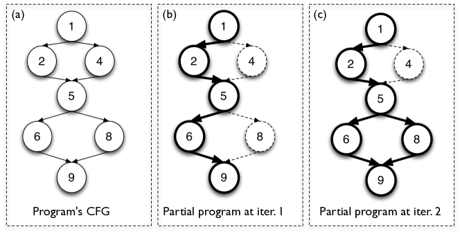
Figure 3: Control flow graph of P (a) and partial P considered during the first (b) and second (c) iteration of OFC.

Step 2 of the algorithm then conjoins input conditions and failing assertion with $TF_{1}$ to obtain the following complete, unsatisfiable formula: $CF_{1}=(x_{1}=0)\wedge(y_{1}=0)\wedge TF_{1}\wedge(b_{3}\leq a_{3})$

The algorithm now marks input clauses, failing assertion, and the two clauses generated from $\phi$ functions as hard clauses, marks all other clauses in $TF_{1}$ as soft clauses, and feeds the result to a pMAX-SAT solver. In this case, the solver would return two CoMSSs: $\{b_{1}=a_{3}+1\}$ and $\{guard_{2}=(y_{1}<5)\}$.

When analyzing the set of clauses in all the CoMSSs, the third step of the algorithm finds that there is one clause associated with a conditional statement $c$ (the one at line $5$, in this case). It thus identifies the branches corresponding to $c$ (i.e., branches $(5,6)$ and $(5,8)$ in the CFG), and checks whether one of the branches was not visited before. This is the case for branch $(5,8)$, so the algorithm selects the unvisited branch as the branch to be expanded and returns to Step 1.

In the second iteration of the algorithm, the Trace Generator re-executes P with the same failing input, but forces the execution to follow branch $(5,8)$ at conditional statement $5$ [37], which results in a new trace: {$1$, $2$, $phi1$, $5$, $8$, $phi2$, $9$}. Given this trace, the algorithm first adds the newly covered program entities to the partial program (see Figure 3(c)) and then computes a new trace formula based on the expanded partial program. Since the execution of statement $8$ instead of statement $6$ is the only difference between this trace and the one generated in the previous iteration, the new trace formula is identical to $TF_{1}$, except for clause $(b_{1}=a_{3}+1)$ (corresponding to statement $6$), which is replaced by clause $(b_{2}=a_{3}+2)$ (corresponding to statement $8$). This trace formula, when conjoint with $TF_{1}$, would thus result in the trace shown below. (In practice, OFC simply conjoins the previous formula and the clause(s) corresponding to the new statement(s), which produces the same result, as explained in Section III-B1.)

$$\scriptstyle\displaystyle TF_{2}= \scriptstyle\displaystyle(guard_{1}=(x_{1}\geq 0))\wedge(a_{1}=x_{1})\wedge$$

$$\scriptstyle\displaystyle((guard_{1}\wedge(a_{3}=a_{1}))\vee(\neg guard_{1}\wedge(a_{3}=a_{2})))\wedge$$

$$\scriptstyle\displaystyle(guard_{2}=(y_{1}<5))\wedge(b_{1}=a_{3}+1)\wedge$$

$$\scriptstyle\displaystyle((guard_{2}\wedge(b_{3}=b_{1}))\vee(\neg guard_{2}\wedge(b_{3}=b_{2})))\wedge(b_{2}=a_{3}+2)$$

Similar to the first iteration, the algorithm then conjoins input conditions ($TF_{2}$) and failing assertion to obtain a new unsatisfiable formula, marks hard and soft clauses, and feeds the formula to the pMAX-SAT solver, which would return two CoMSSs: $\{b_{1}=a_{3}+1\}$ and $\{guard_{2}=(y_{1}<5),b_{2}=a_{3}+2\}$.

Step 3 of the algorithm then checks whether any of these clauses is associated with a conditional statement $cs$ and, if so, whether $cs$ has any outgoing branches not yet visited by a trace. In this case, both of the branches corresponding to the first clause in the second CoMSS have been covered in our analysis. Therefore, the algorithm stops iterating and reports to developers these two CoMSSs, together with their corresponding program entities: $\{$line $6\}$ and $\{$line $5$, line $8\}$.

This would inform developers that suitably changing either (1) the statement at line $6$ or (2) both the conditional statement at line $5$ and the statement at line $8$ could fix the program, so that input ($x_{1}=0$, $y_{1}=0$) would not violate the assertion at line $9$. The clauses associated with the statements would provide additional information that could help understand the fault and find a fix—a (partial) mathematical explanation of how the statements contribute to the failure.

III-B5 Further Considerations

Compared to BugAssist, OFC tends to generate a simpler formula that is as effective as one that encodes the whole program but less expensive to solve. Considering our example, for instance, OFC explored only $2$ of the $4$ paths in the program. Compared to an all-paths analysis, OFC included only relevant program entities in the trace formula: the assertion violation in the example is independent from the outcome of the predicate at statement $1$, and our algorithm successfully identifies the statement as irrelevant and avoids exploring both of its branches. However, although we expect the cost of finding solutions for a formula constructed by OFC to be lower than that of solving the formula generated by an all-paths analysis, OFC can perform a number of iterations when constructing the formula, and thus make multiple calls to the solver. Therefore, whether OFC is more efficient than an all-paths analysis depends on the number and cost of iterations it performs. We study this tradeoff in our empirical evaluation of OFC (see Section IV-B2).

Compared to approaches that consider only the failing trace (e.g., [20, 14]), OFC can conservatively identify all parts of the program that are relevant to the failure. In our example, if the algorithm had stopped after the first iteration, it would have missed the second CoMSS: $\{guard_{2}=(y_{1}<5),b_{2}=a_{3}+2\}$. That is, by reasoning about the original failing trace alone, developers could only infer that the fault may be related to the conditional statement at line $5$. Conversely, by considering also the additional trace, OFC can discover that a fix involving that conditional statement should also consider possible changes to statement $8$. OFC can thus make formula-based debugging more efficient without losing accuracy and effectiveness.

Compared to more traditional debugging techniques, OFC is likely to produce more accurate results. If we applied dynamic slicing to our example, for instance. A dynamic slice computed for the failing assertion at line 9 would include not only statements $5$ and $6$, which is correct, but also statements $1$ and $2$, which are irrelevant for the failure.

III-B6 Additional Details and Optimizations

Handling Multiple Failing Inputs

Although it is defined for a single failing input, OFC can take advantage of the presence of multiple failing tests for the same fault. Because, by definition, the faulty statement(s) should be executed by all failing tests and be responsible for all observed failures, OFC can handle multiple failing inputs as follows: (1) generate a report for each individual failing input, (2) identify the potential faulty entities (and corresponding clauses) that appear in all individual reports, and (3) report to developers only these entities, ranked based on the average of their original ranks in the individual reports.

Loop Unrolling

In the presence of loops, the size of a formula is in general unbounded. As it typical for symbolic analysis approaches (e.g., [15, 31, 26]), in OFC we address this issue by performing loop unrolling [8]. One advantage of OFC over other all-paths analyses is that it can decide how many times to unroll a given loop based on concrete executions, rather than on some arbitrary threshold. Nevertheless, for practicality reason, OFC still needs to define an upper bound for loop unrolling, to limit the overall size of trace formulas.

Dynamic Symbolic Execution

OFC, like dynamic symbolic execution [35, 21], may replace symbolic variables in the trace formula with their corresponding concrete values, so as to allow the solver to handle formulas that go beyond its theories (e.g., non-linear expressions, dynamic memory accesses). Doing so makes the approach more practical, but can introduce unsoundness (in the form of discrepancies between the actual semantics of the program and the semantics encoded in the formula) and reduce the number of possible solutions the solver can compute. This can result in both false positives—program entities that, even if suitably changed, could not eliminate the failure at hand—and false negatives—solutions that do not include the faulty statement(s).

Solution Space Pruning

Because the number of CoMSSs for a given MAX-SAT problem may be too large and affect the ability of OFC to enumerate and analyze all solutions in a reasonable amount of time, OFC allows developers to specify an upper bound for the number of clauses in a CoMSS (i.e., the number of statements reported together as a single fault) and terminates the search for new solutions when the solver starts reporting CoMSSs that exceed this bound. The rationale is that a potential bug generally involves a limited number of statements, whereas a CoMSS that contains a large number of clauses suggests a large semantic change in the program (which may be able to eliminate a failure but is usually not an ideal fix).

IV Empirical Evaluation

To evaluate CW and OFC, we have developed a prototype tool for C programs that implements four different formula-based debugging techniques: BugAssist (BA), BugAssist with clause weighting (BA+CW), on-demand formula computation (OFC), and on-demand formula computation with clause weighting (OFC+CW). We have then empirically investigated the following research questions:

• RQ1: Does BA+CW produce more accurate results than BA? If so, what is CW’s effect on efficiency?

• RQ2: Does OFC improve the efficiency of an all-paths formula-based debugging technique?

• RQ3: Does OFC+CW combine the benefits of OFC and CW? If so, can it scale to programs that an all-paths technique could not handle?

• RQ4: How dependent are our results on the specific solver used?

We now discuss our evaluation setup and our results.

IV-A Evaluation Setup

Implementation

We implemented OFC, as presented in Section III-B, in Java and C. Our tool leverages the LLVM compiler infrastructure (http://llvm.org/) to transform programs into SSA form and add instrumentation that (1) dumps dynamic traces and concrete program states and (2) performs execution hijacking [37] to force the program along specific branches in the Trace Generator. We implemented BA as a version of OFC that builds a formula for all (bounded) paths in the program instead of operating on demand. We implemented Ochiai [5], the statistical fault localization technique that we use for CW, as a Java program that operates directly on the dumped dynamic traces. Finally, to handle wpMAX-SAT and pMAX-SAT problems, we implemented interfaces to invoke the Yices SMT solver [19] and the Z3 theorem prover [4]. We used the Yices solver for the first three research questions, as Z3 does not provide wpMAX-SAT capabilities.

Implementing the OFC algorithm, and in particular the Trace Generator and the Formula Generator components, is extremely challenging both from the conceptual and the engineering standpoint [15]. To avoid spending too much development effort, we decided to build a prototype that implements OFC completely, but has some limitations when handling some constructs of the C language related to heap memory management.

Benchmarks

For our evaluation, we selected three benchmarks. The first two benchmarks consist of multiple (faulty) versions of two programs in the SIR repository [1]: tcas ($41$ versions, ~200 LOC) and tot_info ($11$ versions, ~500 LOC). These programs also come with test cases and a golden (supposedly fault-free) version that can be used as an oracle. We selected these programs for two main reasons. First, tcas is an ideal subject for our evaluation because it allows us to find all possible solutions of the program formulas considered and thus precisely compute the savings that OFC achieves in terms of complexity reduction. (This is in general impossible for larger, more complex programs.) Second, these two programs were also used to evaluate BugAssist [26], which lets us directly compare our results with those of a state-of-the-art all-paths formula-based technique in terms of accuracy and efficiency. The third benchmark we considered is a faulty version of Redis, a widely used in-memory key-value database (~32 KLOC), which also comes with a set of test cases.

Study Protocol

For each faulty program version considered, we proceeded as follows. First, we identified passing and failing test cases for that version. For tcas and tot_info, we did so by defining the assertion for a test using the output generated by the same test when run against the golden implementation. For the bug in Redis, we used the bug description [2] and the corresponding test [3]. We then ran all programs instrumented to collect coverage information for all passing and failing tests at the same time. We used this coverage information to compute the suspiciousness values for the branches and statements in each program version using the Ochiai metric [5]. These are the values that BA+CW and OFC+CW use to assign weights to the clauses in the program formula. Second, for each failing input, we ran all four techniques on the faulty version. Because the all-paths techniques timed out or could not build a formula for the bugs in tot_info and Redis (see Section IV-B3 for details), we could only investigate RQ1 and RQ2 on tcas, whereas we used all three benchmarks for RQ3. (For fairness, we note that Reference [26] reports results for 2 versions of tot_info. However, the authors mention that those results were obtained working on a program slice, and there are no details on how the slice was computed and on which version, so we could not replicate them using either our or their implementation of BA.) For faults with multiple failing test cases, in each technique, we combined the results for the individual inputs, so as to generate a final report for each faulty version and for each technique. For each faulty version and for each technique that successfully ran on it, the technique generated a report for the developers. To do a complete assessment of the performance of the techniques, we also recorded the average CPU time of each technique for each failing input, the number of iterations of the OFC algorithm, whether the generated report contained the fault, and, if so, the rank of the fault in the report.

IV-B Results and Discussion

IV-B1 RQ1—BA+CW Versus BA

To answer this research question, we compared the accuracy and the computational cost of BA+CW and BA to evaluate the impact of leveraging information from statistical fault localization. To do so, we ran both techniques on the $41$ faulty versions of tcas and computed the results as described in Section IV-A. Table I presents these results. The columns in the table show the version ID, the number of lines of code a developer would have to examine before getting to the fault, and the average CPU time consumed by BA and BA+CW to compute their results. For comparison purposes, in the last column we also report the results of a traditional fault-localization technique (Ochiai). For tcas.v3, for instance, it took $292$ seconds (BA) and $183$ seconds (BA+CW) to generate the results, and developers would have to examine $8.5$ lines of code (BA), $1$ line of code (BA+CW), or 3 lines of code (Ochiai). Note that, for BA+CW, the number of lines of code to examine corresponds to the actual rank of the faulty line of code in the report produced by the technique. BA, however, does not rank the potentially faulty lines of code, but simply reports them as an unordered set to developers. Therefore, the number in the table corresponds to the number of lines of code developers would have to investigate if we assume they examine the entities in the set in a random order (i.e., half of the size of the set).

TABLE I: Results for BA and BA+CW when run on tcas.

Version	BA		BA+CW		Ochiai	Version	BA		BA+CW		Ochiai
	rank	time	rank	time	rank		rank	time	rank	time	rank
v1	7.5	26s	2	27s	4	v22	4	7s	5	7s	22
v2	4	15s	4	16s	3	v23	5.5	15s	10	12s	23
v3	8.5	292s	1	183s	3	v24	7.5	30s	8	23s	23
v4	8	11s	3	11s	1	v25	5.5	297s	4	216s	2
v5	7.5	352s	3	323s	18	v26	8	160s	5	123s	21
v6	7.5	569s	5	316s	4	v27	9.5	443s	4	393s	21
v7	8	484s	8	238s	8	v28	5	41s	3	40s	2
v8	7.5	21s	13	18s	48	v29	5	25s	1	27s	20
v9	4.5	18s	10	15s	23	v30	5	11s	6	14s	20
v10	8	125s	3	96s	4	v31	8.5	958s	2	909s	4
v11	5.5	130s	1	91s	21	v32	8.5	171s	1	145s	3
v12	8	22s	11	20s	49	v33	6	79s	1	70s	3
v13	8	24s	7	21s	1	v34	7.5	164s	5	144s	23
v14	7	28s	1	28s	1	v35	5	38s	3	40s	2
v15	6.5	14s	5	14s	21	v36	2.5	19s	1	17s	1
v16	8	331s	12	228s	49	v37	7.5	127s	1	136s	3
v17	8	626s	8	285s	49	v38	6.5	8s	1	8s	2
v18	6	378s	6	245s	49	v39	6	244s	4	272s	2
v19	8	399s	5	167s	49	v40	5.5	219s	3	219s	4
v20	8	504s	8	247s	21	v41	7.5	6s	2	5s	6
v21	7.5	252s	8	194s	21	Average	6.5	187s	4.7	137s	17

As the results in Table I show, both techniques were able to identify the faulty statements for all versions considered. We can also observe that both BA and BA+CW produced overall more accurate results that Ochiai (significance level of 0.05 for both BA and BA+CW for a paired t-test). Although this was not a goal of the study, it provides evidence that formula-based techniques, by reasoning on the semantics of a failing execution, can provide more accurate results than a purely statistical approach. As for the comparison of BA and BA+CW, BA+CW produced better results than BA, with a significance level of 0.05 for a paired t-test. On average, a developer would have to examine $4.7$ statements per fault for BA+CW versus $6.5$ for BA. By leveraging the suspiciousness values computed by statistical fault localization, BA+CW can thus outperform BA in most cases ($33$ out of $41$). For the $8$ cases in which BA+CW did not outperform BA, manual analysis of the results identified one main reason. In some cases, the weights computed by fault localization were too inaccurate and caused the solver to first produce CoMSSs that did not include the actual faulty statements. Despite these negative cases, the overall performance of BA+CW is remarkable and justify the use of statistical fault-localization information. BA+CW ranked the faulty statement first for $9$ out of $41$ versions, among the top $3$ statements in another $8$ cases, and at a position greater than $10$ in only $3$ cases.

The data in Table I also allow us to investigate the second part of RQ1, that is, the effect of CW on efficiency. As we discussed in Section III-A, solving wpMAX-SAT problems may be computationally more expensive than solving a pMAX-SAT problem, so the use of CW may negatively affect the efficiency of formula-based debugging. As the table shows, on average BA+CW performs significantly better than BA (137s versus 187s, significance level of 0.05). Although these results may seem counterintuitive, we discovered that the extra information provided by the weights can in many cases unintentionally help the solver find CoMSSs more efficiently.

In summary, our results provide initial evidence that CW can improve formula-based debugging, both in terms of accuracy and in terms of efficiency.

TABLE II: Performance results for BA and OFC on tcas.

Version	BA	OFC	#Iteration	Time per iteration	Version	BA	OFC	#Iteration	Time per iteration
v1	26s	7s	9	0.8s	v22	7s	6s	13.2	0.4s
v2	15s	38s	12	3.2s	v23	15s	24s	11	2.1s
v3	292s	19s	14	1.4s	v24	30s	7s	10	0.7s
v4	11s	6s	9.2	0.6s	v25	297s	244s	12	20.3s
v5	352s	15s	13.4	1.1s	v26	160s	17s	13	1.3s
v6	569s	17s	13	1.3s	v27	443s	15s	13.4	1.1s
v7	484s	104s	14.8	7.1s	v28	41s	24s	11.2	2.2s
v8	21s	5s	10	0.5s	v29	25s	6s	9.8	0.6s
v9	18s	28s	12	2.4s	v30	11s	24s	11	2.2s
v10	125s	22s	14	1.6s	v31	958s	33s	10.8	3s
v11	130s	11s	8.4	1.3s	v32	171s	14s	13	1.1s
v12	22s	17s	14.2	1.2s	v33	79s	178s	13	13.7s
v13	24s	15s	13.3	1.2s	v34	164s	21s	13	1.6s
v14	28s	20s	13.8	1.4s	v35	38s	22s	14	1.5s
v15	14s	20s	13.2	1.5s	v36	19s	11s	11.2	1s
v16	331s	16s	13	1.2s	v37	127s	251s	14	18s
v17	626s	73s	14.2	5.1s	v38	8s	95s	16	5.9s
v18	378s	96s	13.4	7.2s	v39	244s	213s	12	17.8s
v19	399s	17s	13.2	1.3s	v40	219s	180s	10.4	17.3s
v20	504s	7s	9.4	0.8s	v41	6s	5s	8.2	0.6s
v21	252s	6s	8.8	0.7s	Average	187s	48s	12	4s

IV-B2 RQ2—OFC Versus BA

To investigate RQ2, we compared OFC and BA in terms of efficiency. As we did for RQ1, we ran the two techniques on the $41$ faulty versions of tcas and measured their performance. The results are shown in Table II. The table shows the version ID, the average CPU time spent by BA and OFC, respectively, on each failing input, the number of iterations (i.e., path expansions) of the OFC algorithm, and the average CPU time spent by OFC in each iteration. For example, for a failing input in tcas.v1, it took $26$ seconds (BA) and $7$ seconds (OFC) to generate the results, OFC iterated 9 times, and, for each expansion, it took OFC $0.8$ seconds to find all CoMSS solutions.

The second and fifth columns in the table clearly show that it took considerably less time for the pMAX-SAT solver to find solutions for formulas generated in one iteration of OFC (4 seconds) than for formulas generated by BA (187 seconds). The statistically significant gain of efficiency (significance level of 0.05) is caused, as expected, by the difference in the complexity of the encoded formulas—OFC only encodes the subset of the program relevant to the failure into the formulas passed to the solver, while BA generates a much more complex formula that encodes the semantics of the entire program.

The results in the fourth column of Table II indicate that OFC performed 12 iterations per fault, on average. Therefore, as we discussed in Section III-B5, the benefits of generating a simpler formula were in some cases (e.g., tcas.v2) outweighed by the cost of solving multiple pMAX-SAT problems during on-demand expansion, thus making OFC less efficient than BA. In fact, comparing the results in the second and third columns of the table, we can observe that there were $8$ cases in which OFC performed worse than BA.

Overall, however, OFC was more efficient than BA in $33$ out of $41$ cases and could achieve almost 4X speed-ups on average (48 versus 187 seconds) and over 70X speed-ups in the best case (504 versus 7 seconds). Also in this case, the difference in performance between the two techniques was statistically significant at the 0.05 level.

It is also worth noting that our results on the number of iterations performed by OFC provide some evidence that techniques that operate on a single-trace formula (e.g., [20, 14]) may compute inaccurate results, even when they encode both data- and control-flow information. Because each expansion adds new constraints that must be taken into account in the analysis, limiting the analysis to a single trace is likely to negatively affect the quality of the results.

Finally, as a sanity check, we examined the sets of suspicious entities reported by the two techniques. This examination confirmed that OFC reports the same sets as BA (i.e., the fault-ranking results for OFC were the same as those for BA, shown in Table I). That is, it confirmed that OFC is able to build smaller yet conservative formulas and can thus produce the same result as an approach that encodes the whole program.

In summary, our results for RQ2 provide initial, but clear evidence that OFC can considerably improve the efficiency of formula-based debugging without losing effectiveness with respect to an all-paths technique such as BugAssist.

TABLE III: Average time for processing tcas faults.

BA	BA+CW	OFC	OFC+CW
187s	137s	48s	36s

IV-B3 RQ3—OFC+CW Versus BA, BA+CW, and OFC

To answer the first part of RQ3, we compared the performance of OFC+CW with that of the other three techniques considered, in terms of both accuracy and efficiency, when run on the $41$ tcas versions. For accuracy, we found that the results for OFC+CW, not reported here for brevity, were the same as those listed in the “BA+CW” column of Table I. This is not surprising, as OFC reports the same sets as BA, as we just discussed, and we expect CW to benefit both techniques in the same way. Therefore, the results show that OFC+CW is as accurate as BA+CW and more accurate than BA and OFC.

To compare the efficiency of the four techniques considered, we measured the average CPU time required by the techniques to process one fault in tcas, shown in Table III. As the table shows, for the cases considered, combining OFC and CW can further reduce the cost of formula-based debugging by 25% with respect to OFC and by over 80% with respect to our baseline, BA. Although these are considerable improvements, it is unclear whether they can actually result in more scalable formula-based debugging. This is the focus of the second part of RQ3, which aims to assess the potential increase in scalability that our two improvements can provide.

To answer this part of RQ3, we ran the techniques considered on our other two benchmarks: tot_info and Redis.

tot_info results for RQ3

Unlike tcas, tot_info contains loops, calls to external libraries, and complex floating point computations. (We considered all faults except those directly related to calls to external system libraries, which our current implementation does not handle.) Because of the presence of loops, and as discussed in Section III-B6, we set an upper bound of 5 to the size of clauses in a CoMSS. (We believe 5 is a reasonable value, as it means that the technique would be able to handle all faults that involve up to 5 statements.) As we discussed in Section IV-A, for BA and BA+CW the program formula generated was too large, and the solver was not able to compute the set of CoMSSs within two hours (the time limit we used for the study) for the faults considered. Conversely, OFC and OFC+CW were able to compute a result within the time limit for all faults, which provides initial evidence that our improvements can indeed result in more scalable formula-based techniques. By focusing only on the relevant parts of a failing program and leveraging statistical fault localization, OFC+CW can reduce the complexity of the analysis and successfully diagnose faults that an all-paths technique may not be able to handle. To also assess the accuracy of the produced results, in Table IV we show the results computed by OFC+CW. The columns in the table show the program version and the number of lines of code a developer would have to examine before getting to the fault in that version. As the table shows, OFC+CW was able to rank all $11$ faults within the top $10$ statements in the list reported to the developer, and $4$ of them at the top of the list.

TABLE IV: Ranking results of OFC+CW on tot_info

Version	OFC+CW	Version	OFC+CW	Version	OFC+CW
tot_info.v1	2	tot_info.v14	1	tot_info.v20	3
tot_info.v3	1	tot_info.v15	1	tot_info.v22	6
tot_info.v4	1	tot_info.v16	2	tot_info.v23	8
tot_info.v11	3	tot_info.v18	3

203 #define LUA_CMD_OBJCACHE_SIZE 32
...
206 int j, argc = lua_gettop(lua);
...
214 static robj *cached_objects[LUA_CMD_OBJCACHE_SIZE];
...
218 if (argc == 0) 
...
221  return 1;
222 
...
232  for (j = 0; j < argc; j++) {
233    char *obj_s;
234    size_t obj_len;
236    obj_s = (char*)lua_tolstring(lua,j+1,&obj_len);
237    if (obj_s == NULL) break; /* Not a string. */
    /* Try to use a cached object. */
    /* bug fixes */
240-   if (cached_objects[j] && cached_objects_len[j] >= obj_len) {
240+   if (j < LUA_CMD_OBJCACHE_SIZE && cached_objects[j] &&
241+     cached_objects_len[j] >= obj_len) {
...

Figure 4: Excerpt code of the bug in Redis.

TABLE V: Results for OFC+CW when run on the bug from Redis.

Rank	Source Location	Statement
1	scripting.c:237	if (obj_s == NULL) break;
2	scripting.c:236	obj_s = (char*)lua_tolstring(lua,j+1,&obj_len);
3	scripting.c:232	j++
4	scripting.c:206	int j, argc = lua_gettop(lua);
5	scripting.c:218	if (argc == 0)

Redis results for RQ3

To further assess the scalability of OFC+CW, we run the techniques considered on our third benchmark, a real-world bug [2] in Redis, which is considerably larger and more complex than tcas and tot_info. The bug is a potential buffer overflow in a module of Redis that processes Lua scripts (www.lua.org/) and consists of  1 KLOC). Figure 4 shows an excerpt of the bug. The original version of the code fails to check whether the size of the script from the command line is greater than the size of the memory in which it is stored. If the script is too large, the program generates an out-of-boundary memory access and fails.

We inserted assertions that are triggered when a buffer overflow occurs, and applied OFC+CW to the faulty code. Our tool generated the report shown in Table V, which contains five suspicious statements and program locations. The first entry in our report suggests that a control statement should be changed after line 237 of scripting.c to avoid the out-of-boundary access in the next statement. This is also the location where the developers of Redis fixed the bug [2]. Also in this case, we tried to run the all-paths techniques on the module, but they were not successful. Because BA relies on a static model checker that unrolls loops based on a predetermined (low) bound, whereas the loop in the code needs to be executed a large number of times for the bug to be triggered, BA is unable to build a formula for the failure at hand. Unfortunately, increasing the number of times loops are unrolled is not a viable solution, as it causes the number of encoded paths to explode and results in the solver timing out.

Although this is just one bug in one program, and we cannot claim generality of the results, we find the results very encouraging. They provide evidence that our approach could make formula-based debugging applicable to larger programs and real-world faults.

TABLE VI: Average time for processing tcas faults using BA and OFC and two different solvers.

BA_Yices	BA_Z3	OFC_Yices	OFC_Z3
187s	166s	48s	26s

IV-B4 RQ4—Impact of Solver

RQ4 aims to assess whether our results may depend on the use of a specific solver. (For example, Yices may be optimized for the wpMAX-SAT problem and give an unfair advantage to techniques that use CW.) To answer RQ4, we focused on the results presented in Table III, replaced Yices with another state-of-the-art solver, Z3 [4], and recomputed the results using this new solver. Because Z3 does not currently support wpMAX-SAT, we were only able to use Z3 for the two techniques that do not use CW: BA and OFC. Table VI shows these results, side-by-side with the earlier result we obtained using Yices.

From the results in the table, we can observe different values but a similar trend for the results obtained using the two solvers. In both cases, OFC can significantly improve the efficiency of formula-based debugging (significance level of 0.05). Although this is just one study involving two solvers, and thus we cannot claim general validity of our results, it provides initial evidence that the improvements we measured do not depend on the specific solver used.

IV-C Threats to Validity

In addition to the usual internal and external validity threats, a specific one is that we implemented BugAssist, one of the techniques against which we compare, ourselves. Unfortunately, we were not able to use the command-line implementation of BugAssist from its authors, and the Eclipse plugin was problematic to use in a programmatic way. Moreover, the tool’s source code was not available, which we needed to integrate CW and BugAssist for our evaluation.

Another threat to validity is that we performed our evaluation on two simple programs and a module of a real open source project. Therefore, our results may not generalize. However, our main goal was to investigate whether CW and OFC could improve the state of the art in formula-based debugging, so using the same programs used in related work allowed us to directly compare our techniques with such work.

V Related Work

Our work is closely related to formula-based debugging techniques. In particular, OFC builds on BugAssist [26], which encodes a faulty program as an unsatisfiable Boolean formula, uses a MAX-SAT solver to find maximal sets of satisfiable clauses in this formula, and reports the complement sets of clauses as potential causes of the error. The dual of MAX-SAT, that is the problem of computing minimal unsatisfiable subsets (or unsatisfiable cores), can also be leveraged in a similar way to identify potentially faulty statements, as done by Torlak, Vaziri, and Dolby [36]. This kind of techniques have the advantage of performing debugging in a principled way, but tend to rely on exhaustive exploration of (a bounded version of) the program state, which can dramatically limit their scalability. OFC, by operating on demand, can produce results that are at least as good as those produced by these techniques at a fraction of the cost. Moreover, by working on a single path at a time, OFC can directly benefit from various dynamic optimizations. Finally, CW leverages the additional information provided by passing test cases, which are not considered by most existing techniques in this arena.

Another related approach, called Error Invariants, transforms program entities on a single failing execution into a path formula [20]. This technique leverages Craig interpolants to find the points in the failing trace where the state is modified in a way that affects the final outcome of the execution. The statements in these points are then reported as potential causes of the failure. This technique cannot handle control-flow related faults because, as also recognized by the authors, it does not encode control-flow information in its formula. To address this limitation, in followup work the authors developed a version of their approach that encodes partial control-flow information into the path formula [14]; with this extension, their approach can identify conditional statements that may be the cause of a failure. However, compared to OFC’s approach of suitably encoding SSA’s $\phi$ functions, their approach generates much more complex preconditions, that is, conjunctions of all predicates that a statement is control dependent on. Conversely, our algorithm only needs to encode the predicate that the $\phi$ function is directly dependent on. In addition, the two approaches handle potentially faulty conditional statements very differently. OFC considers additional paths induced by a possible modification of the faulty conditionals, and can therefore identify additional faulty statements along these paths. Their technique simply reports the identified conditionals to developers, who may miss important information and produce a partial, if not incorrect, fix (see Section III-B5).

Our work is also related to statistical fault localization techniques (e.g., [25, 28, 29, 13, 6, 34, 30, 9, 40, 10, 32, 22, 24]). Although efficient, these techniques often produce long lists of program entities with no context information, which can limit their usefulness [33]. In CW, we use the results of statistical fault localization as a starting point to inform formula-based debugging and guide the analysis. As our results show, these can result in considerably more accurate (and more informative) fault-localization results.

Other approaches for identifying potentially faulty statements are static and dynamic slicing [7, 38] and delta debugging [16, 39]. These approaches are orthogonal to ours and to formula-based debugging techniques in general, and can be leveraged to achieve further improvements.

Finally, automated repair techniques (e.g., [18, 27, 23]) are related to our work. However, these techniques are also mostly orthogonal to fault-localization approaches, as they require some form of fault localization as a starting point. (One exception is Angelic Debugging, by Chandra and colleagues [12], which combines fault localization and a limited form of repair.) In this sense, we believe that the information produced by our approach could be used to guide the automated repair generation performed by these techniques, which is something that we plan to investigate in future work.

VI Conclusion and Future Work

We presented clause weighting (CW) and on-demand formula computation (OFC), two ways to improve existing formula-based debugging techniques and mitigate some of their limitations. CW incorporates the (previously ignored) information provided by passing test cases into formula-based debugging techniques to improve their accuracy. OFC is a novel formula-based debugging algorithm that, by operating on demand, can analyze a small fraction of a faulty program and yet compute the same results that would be computed analyzing the whole program, at a much higher cost.

To evaluate CW and OFC, we performed an empirical study. In the study, we assessed the improvements that CW and OFC can achieve over a state-of-the-art formula-based debugging approach. Our results show that CW and OFC can improve the accuracy, efficiency, and scalability of the considered approach. Although our results are still preliminary, we believe that they represent an important first step towards further research in this important and promising area.

Our plans for future work are to perform additional studies, including user studies, to further show the usefulness of our approach. We will also explore the possibility of applying our on-demand algorithm to other types of formula-based techniques, such as those based on single-trace analysis (e.g., [14, 20]), to assess whether we can achieve similar, or even better improvements on such techniques. Finally, we will investigate whether formula-based debugging techniques can help automated program repair. Intuitively, the clauses in the CoMSSs produced by the former should be able to inform and guide the latter in finding or synthesizing suitable repairs.

References

- [1] Software-artifact Infrastructure Repository. http://sir.unl.edu/, Apr. 2012.
- [2] Bug in Redis. https://github.com/antirez/redis/commit/ea0e2524aae1bbd0fa6bd29e1867dc1ca133bfa5, May 2014.
- [3] Test cases for scripting.c in Redis. https://github.com/antirez/redis/blob/7f772355f403a1be9592e60f606d457d117fccc5/tests/unit/scripting.tcl, May 2014.
- [4] Z3. http://z3.codeplex.com/, Apr. 2014.
- [5] R. Abreu, P. Zoeteweij, and A. J. C. v. Gemund. An Evaluation of Similarity Coefficients for Software Fault Localization. In Proc. of the 12th Pacific Rim International Symposium on Dependable Computing, pages 39–46, 2006.
- [6] R. Abreu, P. Zoeteweij, and A. J. C. van Gemund. An Observation-based Model for Fault Localization. In Proc. of the 2008 International Workshop on Dynamic Analysis, pages 64–70, 2008.
- [7] H. Agrawal and J. R. Horgan. Dynamic Program Slicing. In Proc. of the 1990 ACM SIGPLAN Conference on Programming Language Design and Implementation, pages 246–256, 1990.
- [8] A. V. Aho, M. S. Lam, R. Sethi, and J. D. Ullman. Compilers: Principles, Techniques, and Tools (2nd Edition). Addison-Wesley Longman Publishing Co., Inc., Boston, MA, USA, 2006.
- [9] S. Artzi, J. Dolby, F. Tip, and M. Pistoia. Directed Test Generation for Effective Fault Localization. In Proc. of the 19th International Symposium on Software Testing and Analysis, pages 49–60, 2010.
- [10] G. K. Baah, A. Podgurski, and M. J. Harrold. Mitigating the Confounding Effects of Program Dependences for Effective Fault Localization. In Proc. of the 19th ACM SIGSOFT Symposium and the 13th European Conference on Foundations of Software Engineering, pages 146–156, 2011.
- [11] J. Bailey and P. J. Stuckey. Discovery of Minimal Unsatisfiable Subsets of Constraints Using Hitting Set Dualization. In Proc. of the 7th International Conference on Practical Aspects of Declarative Languages, pages 174–186, 2005.
- [12] S. Chandra, E. Torlak, S. Barman, and R. Bodik. Angelic Debugging. In Proc. of the 33rd International Conference on Software Engineering, pages 121–130, 2011.
- [13] M. Y. Chen, E. Kiciman, E. Fratkin, A. Fox, and E. Brewer. Pinpoint: Problem Determination in Large, Dynamic Internet Services. In Proc. of the 2002 International Conference on Dependable Systems and Networks, pages 595–604, 2002.
- [14] J. Christ, E. Ermis, M. Schäf, and T. Wies. Flow-sensitive Fault Localization. In Proc. of the 14th International Conference on Verification, Model Checking, and Abstract Interpretation, 2013.
- [15] E. Clarke, D. Kroening, and F. Lerda. A Tool for Checking ANSI-C Programs. In Proc. of the 10th International Conference on Tools and Algorithms for the Construction and Analysis of Systems, volume 2988, pages 168–176, 2004.
- [16] H. Cleve and A. Zeller. Locating Causes of Program Failures. In Proc. of the 27th International Conference on Software Engineering, pages 342–351, 2005.
- [17] R. Cytron, J. Ferrante, B. K. Rosen, M. N. Wegman, and F. K. Zadeck. Efficiently Computing Static Single Assignment Form and the Control Dependence Graph. ACM Transaction on Programming Languages and Systems, 13(4):451–490, Oct. 1991.
- [18] V. Dallmeier, A. Zeller, and B. Meyer. Generating Fixes from Object Behavior Anomalies. In Proc. of the 24th IEEE International Conference on Automated Software Engineering, pages 550–554. IEEE Computer Society, 2009.
- [19] B. Dutertre and L. de Moura. The YICES SMT Solver. http://yices.csl.sri.com/tool-paper.pdf.
- [20] E. Ermis, M. Schäf, and T. Wies. Error Invariants. In Proc. of the 18th International Symposium on Formal Methods, pages 187–201, 2012.
- [21] P. Godefroid, N. Klarlund, and K. Sen. DART: Directed Automated Random Testing. In Proc. of the 2005 ACM SIGPLAN Conference on Programming Language Design and Implementation, pages 213–223, 2005.
- [22] D. Gopinath, R. Zaeem, and S. Khurshid. Improving the Effectiveness of Spectra-based Fault Localization using Specifications. In Automated Software Engineering (ASE), 2012 Proceedings of the 27th IEEE/ACM International Conference on, pages 40–49, 2012.
- [23] D. Jeffrey, M. Feng, N. Gupta, and R. Gupta. BugFix: A Learning-based Tool to Assist Developers in Fixing Bugs. In Proc. of the 17th International Conference on Program Comprehension, pages 70–79, 2009.
- [24] W. Jin and A. Orso. F3: Fault Localization for Field Failures. In Proc. of the 2013 International Symposium on Software Testing and Analysis, pages 213–223, 2013.
- [25] J. A. Jones, M. J. Harrold, and J. Stasko. Visualization of Test Information to Assist Fault Localization. In Proc. of the 24th International Conference on Software Engineering, pages 467–477, 2002.
- [26] M. Jose and R. Majumdar. Cause Clue Clauses: Error Localization Using Maximum Satisfiability. In Proc. of the 2011 ACM SIGPLAN Conference on Programming Language Design and Implementation, pages 437–446, 2011.
- [27] C. Le Goues, T. Nguyen, S. Forrest, and W. Weimer. GenProg: A Generic Method for Automatic Software Repair. IEEE Transactions on Software Engineering, pages 54 –72, 2012.
- [28] B. Liblit, A. Aiken, A. X. Zheng, and M. I. Jordan. Bug Isolation via Remote Program Sampling. In Proc. of the 2003 ACM SIGPLAN Conference on Programming Language Design and Implementation, pages 141–154, 2003.
- [29] B. Liblit, M. Naik, A. X. Zheng, A. Aiken, and M. I. Jordan. Scalable Statistical Bug Isolation. In Proc. of the 2005 ACM SIGPLAN Conference on Programming Language Design and Implementation, pages 15–26, 2005.
- [30] C. Liu, X. Yan, L. Fei, J. Han, and S. P. Midkiff. SOBER: Statistical Model-based Bug Localization. In Proc. of the 10th European Software Engineering Conference and 13th ACM SIGSOFT Symposium on the Foundations of Software Engineering, pages 286–295, 2005.
- [31] F. Merz, S. Falke, and C. Sinz. LLBMC: Bounded Model Checking of C and C++ Programs Using a Compiler IR. In Proc. of the 4th International Conference on Verified Software: Theories, Tools, Experiments, pages 146–161, 2012.
- [32] L. Naish, H. J. Lee, and K. Ramamohanarao. A Model for Spectra-based Software Diagnosis. ACM Trans. Softw. Eng. Methodol., 20(3):11:1–11:32, Aug. 2011.
- [33] C. Parnin and A. Orso. Are Automated Debugging Techniques Actually Helping Programmers? In Proc. of the 2011 International Symposium on Software Testing and Analysis, pages 199–209, Toronto, Canada, July 2011.
- [34] R. Santelices, J. A. Jones, Y. Yu, and M. J. Harrold. Lightweight Fault-localization Using Multiple Coverage Types. In Proc. of the 31st International Conference on Software Engineering, pages 56–66, 2009.
- [35] K. Sen, D. Marinov, and G. Agha. CUTE: A Concolic Unit Testing Engine for C. In Proc. of the 10th European Software Engineering Conference and 13th ACM SIGSOFT Symposium on the Foundations of Software Engineering, pages 263–272, 2005.
- [36] E. Torlak, M. Vaziri, and J. Dolby. MemSAT: Checking Axiomatic Specifications of Memory Models. In Proc. of the 2010 ACM SIGPLAN Conference on Programming Language Design and Implementation, pages 341–350, 2010.
- [37] P. Tsankov, W. Jin, A. Orso, and S. Sinha. Execution Hijacking: Improving Dynamic Analysis by Flying Off Course. In Proc. of the 4th International Conference on Software Testing, pages 200–209. IEEE, 2011.
- [38] M. Weiser. Program Slicing. In Proc. of the 5th International Conference on Software Engineering, pages 439–449, 1981.
- [39] A. Zeller and R. Hildebrandt. Simplifying and Isolating Failure-Inducing Input. IEEE Transactions on Software Engineering, 28(2):183–200, Feb. 2002.
- [40] Z. Zhang, W. K. Chan, T. H. Tse, B. Jiang, and X. Wang. Capturing Propagation of Infected Program States. In The 7th Joint Meeting of the European Software Engineering Conference and the ACM SIGSOFT Symposium on the Foundations of Software Engineering, pages 43–52, 2009.