Novel Methods for Activity Classification and Occupany Prediction Enabling Fine-grained HVAC Control.

Abstract

Much of the energy consumption in buildings is due to HVAC systems, which has motivated several recent studies on making these systems more energy-efficient. Occupancy and activity are two important aspects, which need to be correctly estimated for optimal HVAC control. However, state-of-the-art methods to estimate occupancy and classify activity require infrastructure and/or wearable sensors which suffers from lower acceptability due to higher cost. Encouragingly, with the advancement of the smartphones, these are becoming more achievable. Most of the existing occupancy estimation techniques have the underlying assumption that the phone is always carried by its user. However, phones are often left at desk while attending meeting or other events, which generates estimation error for the existing phone based occupancy algorithms. Similarly, in the recent days the emerging theory of Sparse Random Classifier (SRC) has been applied for activity classification on smartphone, however, there are rooms to improve the on-phone processing. We propose a novel sensor fusion method which offers almost 100% accuracy for occupancy estimation. We also propose an activity classification algorithm, which offers similar accuracy as of the state-of-the-art SRC algorithms while offering 50% reduction in processing.

1 Introduction

HVAC is a dominant power consumer in commercial buildings. Much efforts have been invested in the past to efficiently control HVAC. Conventionally, most HVAC systems intake temperature and humidity to control cooling [1]. This limitation can often lead to inefficient energy usage. For example, a room might be cooled to a conservative $24^{o}C$ even when it is unoccupied. Similarly, conventional HVAC control strategy does not take into consideration human comfort factors, such as recent physical activity. This can cause discomfort. For example, upon returning to desk after climbing many stairs, worker would like the temperature to be cooler than the conservative set point of $24^{o}C$.

A number of studies have been conducted in the past that attempted to estimate occupancy using sensors spanning motion sensors, RFID and contact sensors. However, introducing additional sensors incur cost of installation and maintenance, especially for large commercial buildings. To alleviate this problem, a number of studies have attempted to use smartphone for occupancy estimation. For example, [2, 3, 4] uses WiFi signal strength to localize the phone. The general control strategy of these methods are, if the phone location is estimated as the office, the HVAC is activated, otherwise the local unit is turned off. However, note that if the phone is left on desk while the person is away, all of these systems will still determine the office space as occupied. This will lead to significant energy wastage. We overcome this challenge in our paper.

A large body of literature can be found which use wearable sensors for activity detection. Given the current advancement in smartphone sensor technology, our objective is to piggyback the activity estimation on the smartphone to save additional expenses of wearable devices. In particular, we propose a Sparse Random Classifier (SRC) [5] based activity classifier, which pave the pathway to featureless classification that is suited to embedded smartphone platform. Notably, a number of attempts [6, 7, 8, 9] have been taken in the past to use SRC for activity classification. However, the key limitations of these approaches is that higher accuracies are obtained when the feature dimension is significantly higher. Higher feature dimension warrants higher processing on embedded platforms, which could potentially interrupt the processing of other applications on the phone. In this paper we seek to address this challenge. We extend the theory of SRC and show that we can achieve similar accuracy as of the existing proposals, however, with half feature dimension.

Our contributions in this paper are as follows:

1. We propose a sensor fusion method that uses sensor feed from phone microphone and phone accelerometer to determine office occupancy when the phone is placed on the office desk. Privacy is a critical issue when using audio data. We preserve privacy by not storing or transiting raw audio data. Features are directly extracted from raw audio data and used for classification.

2. We also propose a extension of the Sparse Random Classifier for physical activity classification on smartphone. Our classifier achieves better accuracy with significantly smaller feature dimension.

3. Experimental results show that our proposed fusion algorithm achieves 100% accuracy in estimating office occupancy. Results also show that our activity classification algorithm offers greater than 95% accuracy with 50% smaller feature dimension compared to the existing methods.

This paper is organized as follows. In the next section (Section 2), after providing some background on SRC, we describe our proposed extension of SRC for activity classification. Then in Section 3, we first describe the Support Vector Regression model for occupancy inference using individual sensing modality. Then we describe our sensor fusion algorithm for occupancy estimation jointly using multi-modal sensing. We then present the experimental results in Section 4 and finally conclude in Section 5.

2 Sparse Random Classifer for Activity Classifcation

2.1 Sparse Random Classifier

The Sparse Random Classifier(SRC) has been developed underpinning the theory of Compressive Sensing (CS) [5]. SRC has been heavily used for classification in the past [10, 11, 12, 13, 14]. The underlying assumption of SRC is that, given sufficient training samples of the $i$th activity class (such as walking or running and os on) $A_{i}=[v_{i,1}+v_{i,2}+...+v_{i,n_{i}}]\in\mathbb{R}^{m\times n_{i}}$, any test object $y\in\mathbb{R}^{m}$ from the same activity class will approximately lie in the linear span of the training samples associated with object $i$. Mathematical representation of this assumption using $\alpha_{i,j}$ as the coefficients can be given by (1).

$$y=A_{i}=[\alpha_{i,1}v_{i,1}+\alpha_{i,2}v_{i,2}+...+\alpha_{i,n_{i}}v_{i,n_{i}}]$$ (1)

However, the membership $i$ of the test sample is unknown primarily, we define a new matrix $A$ for the entire training set was the concentration of the all $n$ training samples of $k$ object classes:

$$A=[A_{1},A_{2},...,A_{k}]=[v_{1,1}+v_{1,2}+...+v_{k,n_{k}}]$$ (2)

Then the linear representation of the training object $y$ can be rewritten in terms of training samples as

$$y=Ax_{0}\in\mathbb{R}^{m}$$ (3)

where $x_{0}=[0,...,0,\alpha_{i,1},...,\alpha_{i,n_{i}},0,...,0]\in\mathbb{R}^{n}]$ is a coefficient vector whose entries are zero except those associated with $i$-class.

The solution $x_{0}$ can be obtained by solving the system of equation $y=Ax$ when $m>n$. However, in reality $m<n$ (we will explain this later in this section), therefore the system is underdetermined. Conventionally, this difficulty is resolved by solving the minimum $\ell_{2}$-norm solution:

$$\hat{x}_{2}=\arg\min||x||_{2}\mbox{ s. t. }Ax=y,$$ (4)

This optimization in (4) can be solved easily by pseudo inverse of A, however, the solution $\hat{x}$ is not informative. This is because we expect the solution to be sparse where only the coefficients related to test object class are non-zero. However, the $\ell_{2}$ norm provides a dense solution with many non-zero entries spanning multiple classes. This motivates us to seek the sparsest solution to $y=Ax$ by solving the following optimization problem:

$$\hat{x}_{0}=\arg\min||x||_{0}\mbox{ s. t. }Ax=y,$$ (5)

Here $||.||_{0}$ denotes the $\ell_{0}$-norm, which counts the number of nonzero entries in a vector. Solution to the above optimization problem provides the optimal solution, however, solving it for an underdetermined system is NP-hard.

Recent development of the theory of compressive sensing and sparse representation has shown that if the solution $x_{0}$ is sparse enough, $\ell_{1}$-minimization provides same solution as that of $\ell_{0}$-minimization:

$$\hat{x}_{1}=\arg\min||x||_{1}\mbox{ s. t. }Ax=y,$$ (6)

In the past a large body of studies have successfully used $\ell_{1}$-minimization to find the sparse solution [15, 16, 17, 18, 19, 20, 21]. This problem can be solved in polynomial time by standard linear programming methods.

2.2 Novel Extension of Sparse Random Classifier for Activity Classification

Recall from the previous section that $m<n$. Here, $n$ is the number of samples in an object instance. For large signals, for example for images, it is the number of pixels in the image vector after vectorization. For instance, if the face images are given at the typical resolution, 640$\times$480 pixels, the dimension $m$ is in the order of $10^{5}$. A higher dimension of the object offers extended processing complexity for regular computers, therefore, embedded platforms are out of question. In order to address this problem projections are taken to transform the images from image space to feature space:

$$Ry=RAx$$ (7)

Here $R\in\mathbb{R}^{d\times n}$ is the so called projection matrix with $d<<n$. In conventional SRC, Gaussian random numbers are used as the elements of $R$. However, we propose a novel construction of projection matrix. We first describe the projection matrix construction method in [Carin:12]. The method assumes that the dictionary $A\in\mathbb{R}^{m\times n}$ and the number of projections $m$ are the inputs. The method first computes the singular value decomposition (SVD) of $A$:

$$D=U\Lambda V^{T}$$ (8)

where ^T denotes matrix transpose, $\Lambda\in\mathbb{R}^{n\times d}$ contains the singular values in its main diagonal, and $U\in\mathbb{R}^{n\times n}$ and $V\in\mathbb{R}^{d\times d}$ are orthonormal matrices. The method in [Carin:12] is to randomly choose $m$ columns from the matrix $U$. Let $\tilde{U}_{m}$ be a $n\times m$ matrix formed by these $m$ randomly chosen columns from $U$. The method is to use $\tilde{U}_{m}^{T}$ as the projection matrix. The rationale of the method is that the columns in $U$ are highly uncorrelated with the dictionary $D$, therefore the sensing matrix $\Psi D=\tilde{U}_{m}^{T}D$ will have low coherence.

In our proposed method, we choose the $m$ columns in $U$ corresponding to the largest $m$ singular values of $D$. We now explain why this is a better choice. To simplify notation, we assume that the SVD in (8) has been permuted so that singular values appear in non-increasing order in the diagonal of $\Lambda$. With this notation, let $U_{m}$ denotes the sub-matrix containing the left-most $m$ columns of $U$; note that these $m$ columns correspond to the largest $m$ singular values of $D$. Our choice of projection matrix is therefore $U_{m}^{T}$.

To understand why $U_{m}$ is a better choice, note that the activity classification problem can be stated as estimating the unknown coefficient vector $s$ from the projection $y$ by solving $y=RAx_{0}$. We assume that the unknown coefficient vector $x_{0}$ comes from some probability distribution such that $\mathbb{E}[x_{0}x_{0}^{T}]=\mathbb{I}$ where $\mathbb{E}$ and $\mathbb{I}$ denote respectively the expectation operator and the identity matrix. It can be shown that the mean signal power $\mathbb{E}[y^{T}y]$ can be written as:

$$\mathbb{E}[y^{T}y]=trace(RU\Lambda^{2}U^{T}R^{T})$$ (9)

If we impose the constraint that each row of the projection matrix $R$ has unit norm, then the $R$ that maximizes $\mathbb{E}[y^{T}y]$ is given by the first $m$ rows of $U^{T}$ (or $U_{m}^{T}$), i.e. the $m$ left singular vectors corresponding to the largest $m$ singular values. This shows that our choice of projection matrix maximises the signal power of $y$. A higher signal power typically translates to lower estimation error.

3 Occupancy Estimation Using Sensor Fusion

When the phone is carried, it can be trivially determined that it is accompanied by its owner. However, in office people often tend to put the phone on desk and work. Further, often they leave the desk while keeping in the phone on it. We consider determining occupancy in these two scenarios. We consider data from the phone accelerometer and the phone microphone to determine occupancy and use a number of assumptions to develop our occupancy estimation algorithm:

1. When people are typing it could create minor acceleration in the phone kept on the table.

2. When the person is not typing, the accelerometer may not be able to pickup the presence, however, sounds of general movement while seated can be picked up by the phone microphone.

3. When people are away from desk, the accelerometer can pickup acceleration from any devices, such as PC or laptop running on the desk.

3.1 Features

3.1.1 Accelerometer

We study three axes of the accelerometer separately. We use a segment size containing one second of data. We investigate mean, 25 and 75 percentile and maximum magnitude of each segment and do not observe any significant difference in classification for those choices. In the results section we use maximum magnitude of each segment as a feature.

3.1.2 Sound

To preserve privacy we refrain using raw audio data for classification. We test the feasibility of signal energy and number of zero crossing as features and find number of zero crossing to be a better choice. Computation of signal energy involves determining a hamming window, which is a resource intensive operation and most importantly it does not provide classification accuracy as good as zero-crossing. We therefore use number of zero crossings as a feature. We investigate on two attributes of audio data to calculate number of zero crossings: 1. sampling frequency and 2. segment size. We test a range of sampling frequencies spanning 8kHz,16kHz,32kHz and 48kHz and find that 48kHz provides the best results. We test window sizes of 5s, 15s, 25s, 35s and 45s and observe that 5s window provides the best results (Results are shown in Section 4).

3.2 Occupancy modeling

Note that prior to applying fusion, we use the classical Support Vector Regression (SVR) for modeling occupancy individually from the audio and accelerometer features discussed in the previous section. The complete description of SVR is outside the scope of this paper. However, in this section we will provide intuition sufficient to understand the working principles of SVR.

3.2.1 Support Vector Regression

Our approach to predicting gait velocity is based on learning the functional relationship between the transition times and gait velocity. To learn this relationship, we used a support vector regression model, which is widely used for prediction [22, 15, 23].

Consider a training set $\{(x_{1},y_{1}),(x_{2},y_{2}),...,(x_{\ell},y_{\ell})\}$, where $x_{i}$s are aggregated accelerometer or acoustic features and $y_{i}$s are the occupancy status. Support vector regression computes the function $f(x)$ that has the largest $\epsilon$ deviation from the actual observed $y_{i}$ for the complete training set.

(a) No relation between $x$ and $y$.

(b) Linear regression.

(c) Linear SVR.

Figure 1: Support vector regression explained.

Let us assume the relationship between the variables is linear of the form $y=\omega x+b$, where $\omega$ (weight vector) and $b$ are parameters to be estimated. Fig. 1(a) shows a few possible linear relationships between the points $x$ and $y$. The solid line in Fig. 1(c) shows the SVR line given by $f(x)=\omega x+b$. The cylindrical area between the dotted lines shows the region without regression error penalty. In the SVR literature this area is considered as the measure of complexity of the regression function used. Points lying outside the cylinder are penalized by an $\epsilon$-insensitive loss function (10) [Vapnik:1995:NSL:211359] given by $|\xi|_{\epsilon}$.

$$|\xi|_{\epsilon}:=\begin{cases}0{\hskip 56.9055pt\mbox{i}f}|\xi|\leq\epsilon\\ |\xi|-\epsilon\mbox{ \hskip 28.45274pt otherwise.}\end{cases}$$ (10)

Now lets us explain the implication of a few different values of $\omega$. In the extreme case when $\omega=0$ (as in Fig. 1(a)), the functional relationship between $x$ and $y$ is least complex or in other words there is no relationship between $x$ and $y$. Therefore the overall error is very high. Next Fig. 1(b) represents the case where the training data fits the solid line quite well. The solid line represents the classical regression analysis, where the loss function is measured as the squared estimation error. Note that although the solid line fits the data well, the cylindrical area between the dotted line is small, which means that the model will not generalize as well in predicting new data. SVR seeks to find a balance between the flatness of the area amongst the dotted lines and the number of training mistakes (see Fig. 1(c)).

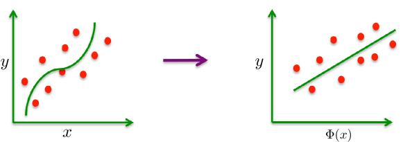
Figure 2: Feature Space Transformation.

Note that in many cases the relationship between the variables is non-linear as shown in the left diagram in Fig. 3. In those cases the SVR method needs to be extended, which is done by transforming $x_{i}$ into a feature space $\Phi(x_{i})$. The feature space linearizes (right diagram in Fig. 3) the relationship between $x_{i}$ and $y_{i}$, therefore, the linear approach can be used to find the regression solution. A mapping function or so called Kernel function is used to transform into feature space. There are four different functions which are frequently used as kernels within support vector regression: linear, RBF (Radial Basis Function), polynomial, and sigmoid. When the feature set is small, the RBF kernel is preferable over others. We use only one feature of transition time, therefore we use the RBF Kernel. However, we empirically verify that the RBF kernel performs better than the linear kernel. There are two parameters, namely $\gamma$ and $C$ (refer to [24] for details) whose values need to be determined for best prediction. Here $C$ is the manually adjustable constant, and $\gamma$ is the kernel parameter which is formally defined as $K(x,y)=e^{-\gamma}||x-y||^{2}$. The overview of our SVR prediction framework is illustrated in Fig. 3.

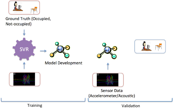
Figure 3: SVR Prediction Framework.

3.3 Sensor Fusion

Since both of the sensor data are simultaneous collected on the phone, we investigate the feasibility of sensor fusion to improve the accuracy of occupancy estimation. Our fusion algorithm is motivated by the Dynamic Weighted Majority (DWM) Voting [25], which is a ensemble learning algorithm. In DWM a series of learning algorithms, namely experts, are used to improve the predictive performance. At the beginning all the experts have equal weights, however, weights are penalized due to wrong prediction. We present a slight modification of the algorithm: we use multiple modalities as experts and use support vector regression for perdition, for each modality. Unlike DWM, we do not remove experts. Our extended Dynamic Weighted Majority Algorithm is presented in Algorithm 1.

At the start of the algorithm both modalities have equal weight of 1. We use a 5-Fold cross validation where in each fold the accelerometer and acoustic features are used separately to predict the occupancy using the SVR model. If the prediction is wrong, weight is reduced by half ($\beta=0.5$) otherwise weight is kept the same. At the end of these 5-Fold cross validation, weights for both modalities are learned and later on used for testing. We learn the weights individually for each subject.

Algorithm 1 Extended Weighted Majority Algorithm

$\{x,y\}_{1}^{n}$: training data, feature vector and class label
$\beta$ : factor for decreasing weights, $0\leq\beta<1$
$c\in N^{*}$: number of classes
$\{e,w\}_{1}^{m}$: set of sensing modalities and their weights
$\sigma\in\mathbb{R}^{c}$: sum of weighted predictions for each class
$\Lambda,\lambda\in{1,...,c}$: global and local predictions

for $i=1,...,n$ do

     $\sigma_{i}\leftarrow 0$

     for $j=1,.....,m$ do

         $\lambda\leftarrow SVR(e_{j},x_{i})$

         if ($\lambda\neq y_{i}$) then

              $w_{j}\leftarrow w_{j}\beta$

         end if

         $\sigma_{\lambda}\leftarrow\sigma_{\lambda}+w_{j}$

     end for

     $\Lambda=\arg\max_{j}\sigma_{j}$

end for

4 Results

4.1 Activity Classification

4.1.1 DataSets

We validate the performance of our proposed $\ell_{1}$ classifier, using publicly available dataset from University of California, Irvine (UCI) [anguita2012human]. In order to create this datasets, experiments were carried out with a group of 30 volunteers within an age bracket of 19-48 years. Each person performed the six activities: standing, walking, laying, walking, walking upstairs and walking downstairs, wearing the a Samsung Galaxy S2 smartphone on the waist. The features selected for this database come from the accelerometer and gyroscope 3-axial raw signals tAcc-XYZ and tGyro-XYZ. These time domain signals (prefix ’t’ to denote time) were captured at a constant rate of 50 Hz. Then they were filtered using a median filter and a 3rd order low pass Butterworth filter with a corner frequency of 20 Hz to remove noise. Similarly, the acceleration signal was then separated into body and gravity acceleration signals (tBodyAcc-XYZ and tGravityAcc-XYZ) using another low pass Butterworth filter with a corner frequency of 0.3 Hz.

Subsequently, the body linear acceleration and angular velocity were derived in time to obtain Jerk signals (tBodyAccJerk-XYZ and tBodyGyroJerk-XYZ). Also the magnitude of these three-dimensional signals were calculated using the Euclidean norm (tBodyAccMag, tGravityAccMag, tBodyAccJerkMag, tBodyGyroMag, tBodyGyroJerkMag).

Finally a Fast Fourier Transform (FFT) was applied to some of these signals producing fBodyAcc-XYZ, fBodyAccJerk-XYZ, fBodyGyro-XYZ, fBodyAccJerkMag, fBodyGyroMag, fBodyGyroJerkMag. (Note the ’f’ to indicate frequency domain signals). In total there were 561 features made available for this dataset. The experiments have been video-recorded to facilitate the data labeling.

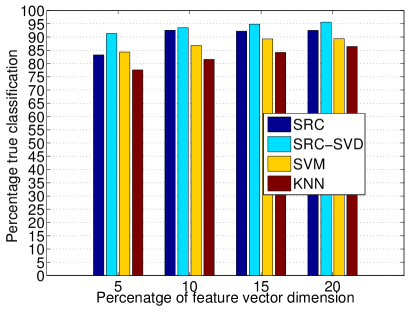
Figure 4: Comparison of $\ell_{1}$-miimization approaches with SVM and kNN. The feature vector consists of 561 attributes.

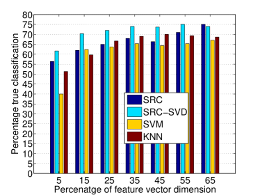
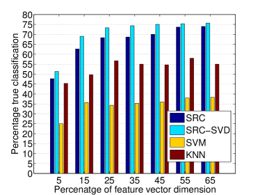
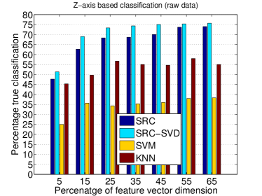
Figure 5: Activity classification using raw data accelerometer data. Feature vector size is 128.

4.2 Activity Classification

The key fundamental aspect of SRC is that it can perform classification with random features or in other words with raw sensor data. Therefore, it is possible to avoid the extensive feature extraction process. However, there is a trade-off between processing and accuracy while choosing between random and sophisticated features, which we present in Fig. 4 and Fig. 5. We call our proposed extension of SRC, SRC-SVD. We benchmark the performance of SRC-SVD upon comparing with three other powerful alternatives: SRC (conventional implementation), Support Vector Machine (SVM) and k-nearest neighbor(kNN).

In Fig 4, the 561 features are used for various classifiers. We apply dimension reduction (using (7)) to the signals. Due to our interest in smaller feature dimension, we present results for 95% to 80% of dimension reduction. We have a number of observations from this figure: 1. in general our proposed SRC-SVD performs the best compared to its alternatives. 2. SRC-SVD performs the best compared to the alternatives when dimension reduction is 95%. 3. Performance of SRC-SVD improves while dimension is increased from 5% to 15%, but plateaus beyond that point. The highest classification accuracy is 95%.

In Fig. 5, we present the classification performance of SRC-SVD to classify using raw accelerometer data. We use all three axes of the accelerometer separately. Similar to Fig. 4, we also compare the performance of SRC-SVD with SRC, SVM and kNN. We observe that 1. SRC-SVD performs the best compared to the other classification methods. 2. X-axis provides the best classification commonly for all classification methods. 3. Classification performance of SRC-SVD increases gradually when dimension increases from 5% to 35% and plateaus beyond that point. The highest classification accuracy achieved is 75%.

4.3 Occupancy Estimaiton

4.3.1 Experimental Settings

Experiments to determine occupancy were conducted with the assistance of three office colleagues. Each of them were given a Nexus 4S smartphone temporarily to collect data about their occupancy. They were allowed to use the phones for personal purpose (day to day usage). The subjects logged the information about their occupancy and location of the phone. We only used the log entries indicating phone on table and in/out of office to validate our occupancy algorithm. There was no information available about how the phone was placed on the table, such as how far from keyboard etc.

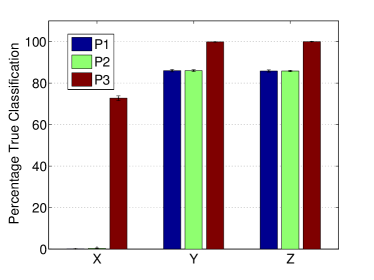
(a) Occupied

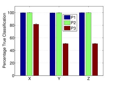
(b) Unoccupied

Figure 6: Occupancy estimation using Accelerometer Data. P1, P2 and P3 are three individual subjects. X, Y and Z corresponds to three axes of the accelerometer. The error bar shows the standard error of the mean. The standard error of the mean now refers to the change in mean with different experiments conducted each time.

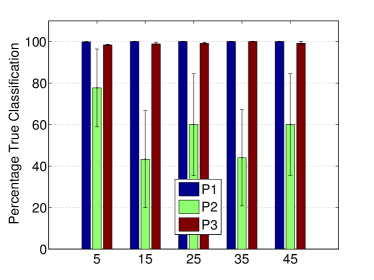
(a) Occupied

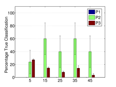
(b) Unoccupied

Figure 7: Occupancy estimation using Microphone Data. P1, P2 and P3 are three individual subjects. X-axis shows the bin size. The error bar shows the standard error of the mean.

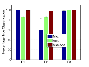
(a) Occupied

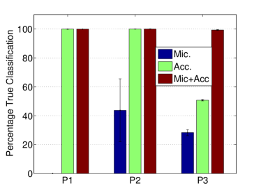
(b) Unoccupied

Figure 8: Comparison amongst single and fused sensing modalities. Z-axis data of the accelerometer and 5s sampling window for microphone have been used. Weighted majority voting has been applied to fuse data from these two modalities. P1, P2 and P3 are three individual subjects. Acc. and Mic. are short form of accelerometer and microphone, respectively.

4.4 Occupancy Estimation Accuracy

The results related to occupancy estimation accuracy are shown in Fig. 6 to Fig. 8. In Fig. 6 we present the accuracy when only accelerometer data is used. When the phone is on the desk, Z-axis is vertical to the desk surface. So, intuitively, most of the acceleration should be experienced along Z-axis. This is also reveled in this figure. For all our subjects, Z-axis provides better accuracy in both occupied and unoccupied cases.

Fig. 7 shows the occupancy estimation performance when using zero crossing as a feature of microphone data. The sound is recorded at 48KHz and we investigate the feasibility of various sampling window, such as 5s, 10s, 15s, and so on as shown in the figure. We observe that 1. microphone is particular suited to determine the occupied case. It performs badly for the unoccupied case and 2. the sampling window of 5s provides the best accuracy.

Given the differential performances of each modality, we investigate the feasibility of joint estimation using both modality. We define a fusion algorithm (Algorithm 1) which is motivated by the Dynamic Weighted Majority Voting. The sensor fusion provides significantly better performance compared to the individual modality in both occupied and unoccupied cases. It can be found from Fig. 8 that for all three subjects and for both occupied and unoccupied cases, the accuracy is almost 100%. We use z-axis data from accelerometer and use a 5s sampling window for the microphone data (sampled at 48KHz) in the sensor fusion algorithm.

5 Conclusions

In this paper we have presented two novel methods for activity classification and occupancy estimation, which are two crucial components for intelligent HVAC control. Physical activities performed recently typically indicate the need for adjusting thermal preferences. Similarly, occupancy is very important in HVAC control. It can save power consumption substantially while maintaing thermal comfort if the HVAC duty cycling can be adapted correctly to the occupancy status.

The novelty of our activity classification algorithm lies in the extension of the Sparse Random Classifier. We introduce a novel construction of projection matrix that offers higher accuracy compared to the conventional implementation of Sparse Random Classifier (SRC). We report that the classification accuracy can be as high as 95% while using 50% smaller feature dimension compared to the existing implementation of SRC.

Our occupancy estimation is novel because, for the first time we propose the fusion of accelerometer and microphone data from smartphone to determine occupancy. We perform experiments with real subjects and experimental results reveal that we achieve almost 100% classification accuracy, which is substantially high. In these experiments accelerometer and microphone data were used when the subject reported that phone was on desk. One of the most important aspects of our experiments is that it was completely uncontrolled. There was no information available on how the phone was placed on the desk, i.e., how far it was placed from the keyboard or hand etc.

In our future studies, we want to validate the proposed sensor fusion algorithm with large number of subjects. In addition, we are also aiming to implement the activity classification algorithm on smartphone and conduct experiments with human subjects to validate its performance.

6 References

References

- [1] A. S. ASHRAE, Standard 90.1-2004, energy standard for buildings except low rise residential buildings, American Society of Heating, Refrigerating and Air-Conditioning Engineers, Inc.
- [2] A. Krioukov, D. Culler, Personal building controls, in: Proceedings of the 11th international conference on Information Processing in Sensor Networks, ACM, 2012, pp. 157–158.
-
[3]
B. Balaji, J. Xu, A. Nwokafor, R. Gupta, Y. Agarwal,
Sentinel: Occupancy based
hvac actuation using existing wifi infrastructure within commercial
buildings, in: Proceedings of the 11th ACM Conference on Embedded Networked
Sensor Systems, SenSys ’13, ACM, New York, NY, USA, 2013, pp. 17:1–17:14.
doi:10.1145/2517351.2517370.
URL http://doi.acm.org/10.1145/2517351.2517370 - [4] K. Christensen, R. Melfi, B. Nordman, B. Rosenblum, R. Viera, Using existing network infrastructure to estimate building occupancy and control plugged–in devices in user workspaces, International Journal of Communication Networks and Distributed Systems 12 (1) (2014) 4–29.
- [5] J. Wright, A. Y. Yang, A. Ganesh, S. S. Sastry, Y. Ma, Robust face recognition via sparse representation, Pattern Analysis and Machine Intelligence, IEEE Transactions on 31 (2) (2009) 210–227.
- [6] M. Zhang, A. A. Sawchuk, Human daily activity recognition with sparse representation using wearable sensors, Biomedical and Health Informatics, IEEE Journal of 17 (3) (2013) 553–560.
- [7] W. Xu, M. Zhang, A. A. Sawchuk, M. Sarrafzadeh, Robust human activity and sensor location corecognition via sparse signal representation, Biomedical Engineering, IEEE Transactions on 59 (11) (2012) 3169–3176.
- [8] C. Liu, Y. Yang, Y. Chen, Human action recognition using sparse representation, in: Intelligent Computing and Intelligent Systems, 2009. ICIS 2009. IEEE International Conference on, Vol. 4, IEEE, 2009, pp. 184–188.
- [9] W. Xu, M. Zhang, A. A. Sawchuk, M. Sarrafzadeh, Co-recognition of human activity and sensor location via compressed sensing in wearable body sensor networks, in: Wearable and Implantable Body Sensor Networks (BSN), 2012 Ninth International Conference on, IEEE, 2012, pp. 124–129.
- [10] S. Sivapalan, R. K. Rana, D. Chen, S. Sridharan, S. Denmon, C. Fookes, Compressive sensing for gait recognition, in: Digital Image Computing Techniques and Applications (DICTA), 2011 International Conference on, IEEE, 2011, pp. 567–571.
- [11] S. W. Chew, R. Rana, P. Lucey, S. Lucey, S. Sridharan, Sparse temporal representations for facial expression recognition, in: Advances in Image and Video Technology, Springer, 2012, pp. 311–322.
- [12] B. Wei, M. Yang, Y. Shen, R. Rana, C. T. Chou, W. Hu, Real-time classification via sparse representation in acoustic sensor networks, in: Proceedings of the 11th ACM Conference on Embedded Networked Sensor Systems, ACM, 2013, p. 21.
- [13] J. Xu, S. Denman, S. Sridharan, C. Fookes, R. Rana, Dynamic texture reconstruction from sparse codes for unusual event detection in crowded scenes, in: Proceedings of the 2011 joint ACM workshop on Modeling and representing events, ACM, 2011, pp. 25–30.
-
[14]
B. Wei, M. Yang, R. K. Rana, C. T. Chou, W. Hu,
Distributed sparse
approximation for frog sound classification, in: Proceedings of the 11th
International Conference on Information Processing in Sensor Networks, IPSN
’12, ACM, New York, NY, USA, 2012, pp. 105–106.
doi:10.1145/2185677.2185699.
URL http://doi.acm.org/10.1145/2185677.2185699 - [15] R. Rana, W. Hu, T. Wark, C. T. Chou, An adaptive algorithm for compressive approximation of trajectory (aacat) for delay tolerant networks, in: Wireless Sensor Networks, Springer, 2011, pp. 33–48.
- [16] R. K. Rana, C. T. Chou, S. S. Kanhere, N. Bulusu, W. Hu, Ear-phone: an end-to-end participatory urban noise mapping system, in: IPSN ’10: Proceedings of the 9th ACM/IEEE International Conference on Information Processing in Sensor Networks, ACM, New York, NY, USA, 2010, pp. 105–116. doi:http://doi.acm.org/10.1145/1791212.1791226.
- [17] R. Rana, C. T. Chou, W. Hu, Energy-aware sparse approximation technique (east) for rechargeable wireless sensor networks., in: Proceedings of the seventh European Conference on Wireless Sensor Network (EWSN 2010), Coimbra, Portugal, 2010, pp. 306–321.
- [18] Y. Shen, W. Hu, R. Rana, C. T. Chou, Nonuniform compressive sensing for heterogeneous wireless sensor networks, IEEE SENSORS JOURNAL 13 (6) (2013) 2120–2128.
- [19] C. Chou, W. Hu, et al., Efficient computation of robust average of compressive sensing data in wireless sensor networks in the presence of sensor faults.
- [20] C. T. Chou, R. Rana, W. Hu, Energy efficient information collection in wireless sensor networks using adative compressive sensing., in: Proceedings of LCN 2009: The 34th IEEE Conference on Local Computer Networks, Zurich, Switzerland, 2009, pp. 443–450.
- [21] Y. Shen, W. Hu, R. Rana, C. T. Chou, Non-uniform compressive sensing in wireless sensor networks: Feasibility and application, in: Intelligent Sensors, Sensor Networks and Information Processing (ISSNIP), 2011 Seventh International Conference on, IEEE, 2011, pp. 271–276.
- [22] R. Rana, B. Kusy, R. Jurdak, J. Wall, W. Hu, Feasibility analysis of using humidex as an indoor thermal comfort predictor, Energy and Buildings.
- [23] R. Rana, D. Austin, P. G. Jacobs, M. Karunanithi, J. Kaye, Passive in-home estimation of gait velocity from motion sensors, arXiv preprint arXiv:1310.4880.
- [24] C.-C. Chang, C.-J. Lin, Libsvm: a library for support vector machines, ACM Transactions on Intelligent Systems and Technology (TIST) 2 (3) (2011) 27.
- [25] J. Z. Kolter, M. Maloof, Dynamic weighted majority: A new ensemble method for tracking concept drift, in: Data Mining, 2003. ICDM 2003. Third IEEE International Conference on, IEEE, 2003, pp. 123–130.