Edge binding of sine-Gordon solitons in spin-orbit coupled Bose-Einstein condensates

Abstract

In recent experiments with ultracold gases a Raman coupling scheme is used to produce both spin-orbit (SO) and Zeeman-type couplings [Y.-J. Lin et al., Nature 471, 83 (2011)]. Their competition drives a phase transition to a magnetized state with broken $Z_{2}$ symmetry. Using a hydrodynamic approach we study a confined binary condensate subject to both SO and Zeeman-type couplings. We find that in the limit of small healing length and in the phase with unbroken symmetry, the boundary magnetization profile has an analytical solution in the form of a sine-Gordon soliton. The soliton is bound to the edge of the system by the nontrivial boundary condition resulting from the combined effect of the SO coupling and the drop in the particle density. The same boundary condition is important in the magnetized phase as well, where we characterize numerically the boundary spin structure. We further discuss how the nontrivial magnetization structure affects the density profile near the boundary, yet another prediction that can be tested in current experiments of spin-orbit coupled condensates.

Introduction — Ultracold atomic gases allow a relatively easy way to study several phenomena that are difficult to probe in solid-state systems Bloch:2008 ; Nori:2014 . Of particular note are those phenomena associated with spin-orbit (SO) coupling, which has been artificially engineered in a Bose-Einstein condensate (BECs) in Ref. Lin:2011, using a Raman laser scheme Goldman:2013 . This opens up the possibility of exploring the physics of bosons with SO coupling that was previously inaccessible.

In addition to the SO coupling, however, present laser schemes introduce also a finite Zeeman-type coupling Lin:2011 ; Wang:2012 ; Cheuk:2012 ; Zhang:2012a ; Goldman:2013 . While the SO coupling strength can be tuned only by changing the angle between the two Raman beams, the Zeeman-type field (ZF) is controlled by the intensity of the laser beams. It follows that the two couplings cannot be separated. Their interplay manifests in a number of interesting effects, such as dipole oscillations Zhang:2012a ; Li:2012a , Zitterbewegung Zhang:2012b ; Qu:2013 ; LeBlanc:2013 , pairing in Fermi gases Fu:2013 , phase transitions Stanescu:2008 ; Wang:2010 ; Ho:2011 ; Li:2012b ; Ozawa:2013a , excitation spectrum Martone:2012 ; Li:2013 , break-down of Galilean invariance Ozawa:2013b and solitary waves Merkl:2010 ; Zulicke:2012 ; Achilleos:2013 , to mention a few. More details can be found in up-to-date reviews soc_reviews .

Interestingly, in the solid state, it was already noticed that strong SO coupling and Zeeman gap (opened by an external magnetic field) are important ingredients for realizing exotic localized boundary states in nanowires Lutchyn:2010 ; Oreg:2010 . However, the same type of analysis has not yet been considered in the context of cold gases (see however Ref. Baym:2012, ).

In this Letter we focus on the boundary structure of BECs subject to both SO coupling and ZF. By means of a hydrodynamic approach Lamacraft:2008 ; Refael:2009 ; Han:2012 we first recover the $Z_{2}$ symmetry breaking transition driven by the competition between SO and ZF Lin:2011 ; Zhang:2013 . Next, we investigate the peculiar magnetization structure at the boundaries of a condensate confined by a box potential as realized in Ref. Hadzibabic:2013, ; Hadzibabic:2014,  foot4 . In the limit where the healing length $\xi$ is small compared to the typical length scale $\ell_{s}$ of the spin degrees of freedom (defined below) the magnetization is controlled by a modified $O(3)$ sigma model with a boundary condition of the Neumann type induced by the sharp density drop at the potential step. Below the critical value of the SO coupling strength the boundary magnetization has the simple analytical form of a sine-Gordon soliton, which is bound to the edge due to the boundary condition above. The numerical solution of the Gross-Pitaevskii equation confirms that this solution is exact in the limit $\xi/\ell_{s}\to 0$. In the broken symmetry phase the boundary structure can be analysed only numerically taking into account the same boundary condition. Finally, we study how the magnetization structure at the edges affects the density profile to the next leading order in $\xi/\ell_{s}$. All of our predictions are easily accessible experimentally in current cold gases schemes with artificial SO coupling Lin:2011 and confined box-shaped potentials Hadzibabic:2013 ; Hadzibabic:2014 .

Model system and hydrodynamic equations — We use the standard single-particle Hamiltonian with SO coupling induced by Raman lasers Lin:2011 ; soc_reviews

$$H_{\text{s.p.}}=-\frac{\hbar^{2}}{2m}\nabla_{\bm{\mathrm{r}}}^{2}-i\hbar\gamma\sigma_{z}\partial_{x}-\frac{\hbar\Omega}{2}\sigma_{x}+V(\bm{\mathrm{r}})\,.$$ (1)

The SO coupling strength $\gamma$ is given by $\gamma=\hbar k_{L}/m$ with $k_{L}$ the modulus of the difference of the Raman lasers wavevectors Lin:2011 ; Goldman:2013 . The Raman coupling $\Omega$ introduces the Zeeman term $\frac{1}{2}\hbar\Omega\sigma_{x}$, $\sigma_{x,z}$ are the Pauli matrices, and $V(\bm{\mathrm{r}})$ is the external potential.

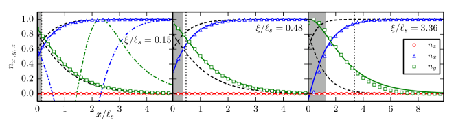
Figure 1: (Color online) The magnetization obtained by imaginary-time evolution of the Gross-Pitaveskii equation (2) is compared to the analytical formulas (10)-(11) for $\xi/\ell_{s}=0.15$ (left panel), $\xi/\ell_{s}=0.48$ (center panel) and $\xi/\ell_{s}=3.36$ (right panel), while $c=0.9$ in all panels. The triangles, squares and circles are respectively the $x,\,y,\,z$ components of the magnetization $\bm{\mathrm{n}}(x)$ obtained numerically, while the solid lines are fits of the function $\phi_{-}(x-\xi^{*},\ell_{s}^{*})$ [Eqs. (10)-(11) and $x_{0}=x_{0,+}$] with fit parameters $\xi^{*}$ and $\ell_{s}^{*}$: $\xi^{*}/\xi=0.92$, $\ell_{s}^{*}/\ell_{s}=1.01$ (left panel); $\xi^{*}/\xi=0.75$, $\ell_{s}^{*}/\ell_{s}=1.08$ (center); $\xi^{*}/\xi=0.37$, $\ell_{s}^{*}/\ell_{s}=2.05$ (right). The black dashed lines are the components $n_{x}$ and $n_{y}$ obtained from Eq. (10)-(11) without fitting ($\xi^{*}=0$ and $\ell_{s}^{*}=\ell_{s}$). The healing length $\xi$ is indicated by a vertical dotted line, while the grey area on the left of the panels has a width equal to $\xi^{*}$. The dashed-dotted lines in the left panel represent the solution corresponding to $x_{0,-}$ in Eq. (11).

Interactions are accounted for at the mean field level by the Gross-Pitaevskii equation (GPE) Goldman:2013 ; soc_reviews

$$i\hbar\partial_{t}\Psi=H_{\text{s.p.}}\Psi+g|\Psi|^{2}\Psi\,,$$ (2)

which is a dynamical equation for the two-component (pseudospin-1/2) complex order parameter $\Psi(\bm{\mathrm{r}})=(\Psi_{\uparrow}(\bm{\mathrm{r}}),\Psi_{\downarrow}(\bm{\mathrm{r}}))$, and $H_{\text{s.p.}}$ is the Hamiltonian (1). The interaction term is isotropic in spin space, a good approximation for experiments Lin:2011 ; Khamehchi:2014 , and is parametrized by the coupling constant $g$.

The condensed gas can be equivalently described by a complete set of gauge invariant quantities such as particle density $\rho(\bm{\mathrm{r}})$, velocity field $\bm{\mathrm{v}}(\bm{\mathrm{r}})$ foot1 and magnetization vector $\bm{\mathrm{n}}(\bm{\mathrm{r}})\,\,(\bm{\mathrm{n}}\cdot\bm{\mathrm{n}}=1)$. This is the so-called hydrodynamic approach which has been introduced in Ref. Lamacraft:2008 ; Refael:2009 for a spinor condensate and in Ref. Han:2012 for the case of an isotropic Dresselhaus SO term. The case of one dimensional SO as in Eq. (1), is a straightforward generalization foot2 , thus only the final result is reported in the following. After parametrizing the magnetization as $\bm{\mathrm{n}}(\bm{\mathrm{r}})=(\sin\theta(\bm{\mathrm{r}})\cos\phi(\bm{\mathrm{r}}),\sin\theta(\bm{\mathrm{r}})\sin\phi(\bm{\mathrm{r}}),\cos\theta(\bm{\mathrm{r}}))$, where $\theta$ and $\phi$ are the polar an azimuthal angles, respectively, the energy functional of the condensate at rest — i.e. with $\bm{\mathrm{v}}=0$, $\partial_{t}\rho=0$ and $\partial_{t}\bm{\mathrm{n}}=0$ — reads

$$E=\int d^{3}x\left[\frac{g\rho^{2}}{2}+V\rho+\frac{(\hbar\nabla\sqrt{\rho})^{2}}{2m}+\rho H_{\sigma}\right]\,,$$ (3)

$$H_{\sigma}=\frac{\hbar^{2}}{4m}\left[\frac{\left(\bm{\mathrm{\nabla}}\theta\right)^{2}}{2}+\frac{\sin^{2}\theta}{2}\left(\bm{\mathrm{\nabla}}\phi+\frac{c}{\ell_{s}}\hat{x}\right)^{2}-\frac{\sin\theta\cos\phi}{\ell_{s}^{2}}\right].$$ (4)

The spin length scale   $\ell_{s}=\sqrt{\hbar/(2m\Omega)}$ and the reduced SO coupling strength $c=\gamma/\gamma_{\text{crit}}$ have been introduced, with $\gamma_{\text{crit}}=\sqrt{\hbar\Omega/2m}$ the SO coupling critical value. $H_{\sigma}$ is the part of the energy functional that depends only on the magnetization and can be identified with the Hamitonian density of a $O(3)$ nonlinear sigma model Rajaraman:1982 modified by SO coupling and ZF. In a homogeneous system the minimum of energy is reached for constant density $\rho(\bm{\mathrm{r}})=\bar{\rho}$ and $\phi=0$, while $\sin\theta=1$ for $\gamma\leq\gamma_{\text{crit}}$ and $\sin\theta=1/c^{2}$ for $\gamma>\gamma_{\text{crit}}$. In the latter case, $n_{z}$ has two possible values, $n_{z}=\pm\sqrt{1-1/c^{4}}$. Therefore the $Z_{2}$ symmetry of the Hamiltonian under the transformation $\sigma_{z}\to-\sigma_{z}$ and $x\to-x$ is broken. This corresponds precisely to the phase transition resulting from the competition of the ZF and the SO coupling Lin:2011 ; soc_reviews . In the following we consider the cases $\gamma\leq\gamma_{\text{crit}}$ and $\gamma>\gamma_{\text{crit}}$ separately.

The $\gamma\leq\gamma_{\text{crit}}$ case — When $\gamma\leq\gamma_{\text{crit}}$ we assume the condition $\sin\theta=1$ ($n_{z}=0$) for a inhomogeneous system as well and consider a translational invariant system in the $y$ and $z$ directions. The two Euler-Lagrange equations obtained by varying the energy functional (3)-(4) are

$$g\rho-\frac{\hbar^{2}\partial_{x}^{2}\sqrt{\rho}}{2m\sqrt{\rho}}+\frac{\hbar^{2}}{4m}\left[\frac{1}{2}\left(\partial_{x}\phi+\frac{c}{\ell_{s}}\right)^{2}-\frac{\cos\phi}{\ell_{s}^{2}}\right]=V\,,$$ (5)

$$\frac{\hbar^{2}}{4m}\left[\partial^{2}_{x}\phi+\frac{\partial_{x}\rho}{\rho}\left(\partial_{x}\phi+\frac{c}{\ell_{s}}\right)\right]=\frac{\hbar\Omega}{2}\sin\phi\,.$$ (6)

For $c=0$ the last two terms on the left-hand side of Eq. (5) form together the sine-Gordon Hamiltonian density. Eq. (6) is precisely the static sine-Gordon equation with an additional term $\propto\partial_{x}\rho/\rho$ on the left hand side.

In the limit of very large interaction strength $g$, the density $\rho$ and the angle $\phi$ in Eqs. (5)-(6) decouple since the density is very stiff and slightly affected by a nonuniform magnetization. This can be shown by considering a hard-wall confining potential of the form $V(x\geq 0)=\mu$, $V(x<0)=+\infty$ at the left boundary. The solutions of Eq. (5), neglecting the $\phi$-dependent part, is

$$\rho_{0}(x)=\bar{\rho}\tanh^{2}\frac{x}{\xi}\qquad\text{for}\quad x\geq 0\,.$$ (7)

The scale of density variation is the healing length $\xi=\sqrt{\hbar^{2}/(m\mu)}$ and $\bar{\rho}=\mu/g$ is the background density far from the boundary. The limit of $\partial_{x}\rho_{0}/\rho_{0}$ for $\xi\to 0$ ($g\to+\infty$) is a discontinuous function foot5

$$\lim_{\xi\to 0}\frac{\partial_{x}\rho_{0}}{\rho_{0}}=\begin{cases}+\infty,&x=0\,,\\ 0,&x>0\,.\end{cases}$$ (8)

Therefore, Eq. (6) reduces to a pure sine-Gordon equation $\partial_{x}^{2}\phi=\sin\phi/\ell^{2}_{s}$ with the non-trivial boundary condition

$$\left.\partial_{x}\phi\right|_{x=0}=-\frac{c}{\ell_{s}}=-\frac{2m\gamma}{\hbar}\,.$$ (9)

The localized solutions of the sine-Gordon equation have the form Rajaraman:1982 ; Manton:2004

$$\phi_{\pm}(x,\ell_{s})=\pm 4\arctan e^{(x+x_{0})/\ell_{s}}\,,$$ (10)

and are called the soliton ($\phi_{+}$) and antisoliton ($\phi_{-}$), respectively. The (anti-)soliton solution is parametrized by the coordinate $-x_{0}$ of the “center of mass”because of the translationally invariance of the sine-Gordon equation. Translational invariance is broken at the boundary and in fact the boundary condition (9) can be satisfied for $\gamma>0$ by the antisoliton solution ($\phi_{-}$) with center of mass coordinate of the form

$$x_{0,\pm}=\ell_{s}\ln\left(2c^{-1}\pm\sqrt{4c^{-2}-1}\right)\,.$$ (11)

The ground state solution for the left boundary is the one corresponding to the plus sign in Eq. (11) since it is continuously connected to the correct ground state in the small SO coupling limit. Moreover, it is easy to verify that this solution has lower energy with respect to the other one. The solution with minus sign in Eq. (11) corresponds to the right boundary. In the following we consider only the left boundary and we take $x_{0}=x_{0,+}$.

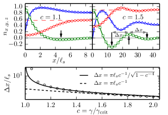
Figure 2: (Color online) Upper panel: Components of the magnetization $n_{x}$ (triangles), $n_{y}$ (squares) and $n_{z}$ (circles) obtained by numerical solution of the GPE in the case $\gamma>\gamma_{\text{crit}}$, while the solid lines are the corresponding solutions that minimize the modified nonlinear sigma model (4) with the boundary conditions $\partial_{x}\theta|_{x=0}=0$ and Eq. (9), shifted to the right by $\xi$ (without fitting). Two values of the SOC have been considered: $c=1.1$ (left upper panel) and $c=1.5$ (right upper panel), while $\xi/\ell_{s}=0.15$ in both panels. The dashed horizontal lines denote the non-zero asymptotic value of $n_{z}(x)$ ($\,n_{z}|_{x\to+\infty}=\sqrt{1-1/c^{4}}\,$), while the arrows correspond to the minima and maxima of $n_{y}(x)$. Lower panel: The circles are the distance $\Delta x$ between the first minimum and the neighbouring maximum of $n_{y}$ as function of $c$ above the critical point, while the solid (dashed) line is the analytic form of the spin-precession length calculated with (without) the ZF. The expression including the ZF is closer to the numerical data.

Eqs. (10)-(11) provide an analytical form for the magnetization profile at the left boundary of the system when $c<1$. We provide below numerical and analytical arguments showing that this solution is in fact exact in the $\xi/\ell_{s}\to 0$ limit. Moreover we show numerically that it captures approximately the magnetization profile in the regime $\xi\lesssim\ell_{s}$. To this end, we consider the solution (10)-(11) as a fitting function $\phi_{-}(x-\xi^{*},\ell_{s}^{*})$ where the fitting parameters $\xi^{*}$ and $\ell_{s}^{*}$ allow for translation and rescaling, respectively. This function is fitted to the numerical solution of the GPE (2) foot3 for three different values of the ratio $\xi/\ell_{s}$, namely $\xi/\ell_{s}=0.15,\,\,0.48,\,\,3.36$, while $c=\gamma/\gamma_{\text{crit}}=0.9$ is fixed, and the results are shown in Fig. 1. For $\xi/\ell_{s}\ll 1$ the agreement with the numerical data is excellent with $\xi^{*}$ and $\ell_{s}^{*}$ very close to $\xi$ and $\ell_{s}$, respectively. The fact that $\xi^{*}\sim\xi$ is expected since in the derivation of Eqs. (10)-(11) we neglected that the density drops to zero on a finite width $\xi$ at the boundary. As shown in Fig. 1 the fitted solution is a very good approximation for $\xi\lesssim\ell_{s}$, while for $\xi>\ell_{s}$ some deviations are noticeable. With increasing ratio $\xi/\ell_{s}$ the fitted value $\xi^{*}$ tends to decrease while $\ell_{s}^{*}$ tends to increase. We have obtained similar results in the whole range $0\leq c\leq 1$. Within numerical precision we conclude that the solution (10)-(11) is exact in the limit $\xi/\ell_{s}\to 0$ $(g\to+\infty)$ limit, and that for finite $g$ the assumption $n_{z}=0$ holds. The same results apply for the right boundary with the only difference that $x_{0,+}\to x_{0,-}$ and consequently $n_{y}\to-n_{y}$.

The $\gamma>\gamma_{\text{crit}}$ case — For $\gamma>\gamma_{\text{crit}}$ we are not able to provide an analytical solution in the limit $\xi/\ell_{s}\to 0$, but we can still minimize numerically the functional in Eq. (4) with the proper boundary condition. One easily finds that the boundary condition $\partial_{x}\theta|_{x=0}=0$ needs to be enforced in addition to Eq. (9). In the upper panel of Fig. 2 we show the boundary structure of a condensate with SO coupling strength $c=1.1$ (left) and $c=1.5$ (right). The solutions of the nonlinear sigma model are shown as lines in Fig. 2 (upper panel). These have been shifted by $\xi$ and provide a significantly better agreement with the full solution of the GPE, as in the case $\gamma\leq\gamma_{\text{crit}}$.

New features for $\gamma>\gamma_{\text{crit}}$ are: i) $n_{z}(x)$ is non-uniform and increases from $n_{z}(x=0)>0$ up to its asymptotic value on a length scale that increases when approaching the critical point; ii) oscillations in all the magnetization components appear. We also found that the distance between the first minimum of $n_{y}$ and the neighbouring maximum is given, to a good approximation, by the spin-precession length Datta:1990 , which is the wavelength corresponding to the minima of the dispersion of $H_{\text{s.p.}}$ (1). The expression for the spin-precession length is provided in the legend of Fig. 2 (lower panel).

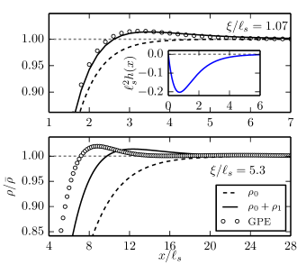
Figure 3: (Color online) Density profiles obtained by means of the GPE (circles) compared to the zero order result $\rho_{0}$ (7) (dashed line) and to the first order one $\rho_{0}+\rho_{1}$ (12) (solid line). Two different values of the ratio $\xi/\ell_{s}$ are considered: $\xi/\ell_{s}=1.07$ (upper panel) and $\xi/\ell_{s}=5.3$ (lower panel). The reduced SO coupling strength is $c=0.9$ as in Fig. 1. The energy density $h(x)$ has been calculated with the function $\phi_{-}(x-\xi^{*},\xi^{*}_{s})$ fitted as in Fig. 1 [fit parameters $\xi^{*}/\xi=0.68$, $\ell_{s}^{*}/\ell_{s}=1.26$ (upper); $\xi^{*}/\xi=0.27$, $\ell_{s}^{*}/\ell_{s}=2.45$ (lower)]. In inset the energy density $h(x)$ in Eq. (13) is shown.

Density profile — In the previous discussion we have assumed the density profile at the boundary to be as in Eq. (7), namely unaffected by the magnetization. We now provide an estimate of the back-action of the non-trivial magnetization structure at the boundary on the density profile, thereby rigorously justifying the result of Eqs. (7)-(11). The first order correction $\rho_{1}(x)$ to Eq. (7) can be expressed as

$$\frac{\rho_{1}(x)}{\bar{\rho}}=-\xi^{2}\tanh\frac{x}{\xi}\int_{0}^{+\infty}dz\,G(x/\xi,z)\tanh(z)\,h(\xi z)\,.$$ (12)

Here we use the dimensionless variable $z=x/\xi$ and $G(z,z^{\prime})$ is the Green’s function of the differential operator $\mathcal{L}=-\frac{d^{2}}{dz^{2}}+2(3\tanh^{2}z-1)$, which is obtained by linearizing Eq. (5) around the equilibrium solution (7). The Green’s function has the form $G(z,z^{\prime})=G(z^{\prime},z)=y_{1}(z)y_{2}(z^{\prime})$ for $z>z^{\prime}$ with $y_{i}(z)$ satisfying $\mathcal{L}\,y_{i}(z)=0$, $y_{1}\sim e^{-2z}$ for $z\to+\infty$, $y_{2}(0)=0$ and $\frac{dy_{2}}{dz}(0)=\frac{1}{y_{1}(0)}$. The energy density $h(x)=\frac{4m}{\hbar^{2}}H_{\sigma}(x)$ (4) enters Eq. (12) and for the sine-Gordon soliton (10) it reads (constant terms are reabsorbed in the chemical potential)

$$h(x)=\frac{4}{\ell_{s}^{2}\cosh\frac{x+x_{0}}{\ell_{s}}}\left(\frac{1}{\cosh\frac{x+x_{0}}{\ell_{s}}}-\frac{1}{\cosh\frac{x_{0}}{\ell_{s}}}\right)\,.$$ (13)

Since the Green’s function can be roughly approximated by the asymptotic form $G(z,z^{\prime})=e^{-2|z-z^{\prime}|}/2$, Eqs. (12)-(13) show that the correction is first order in the expansion parameter $(\xi/\ell_{s})^{2}=2\hbar\Omega/\mu$.

In Fig. 3 the possible approximations to the exact density profiles are compared. The first order correction is already able to capture the characteristic non-monotonic behavior of the density near the boundary. The density bump visible in Fig. 3 matches the energy density of the soliton which is negative and strongly localized (see inset of Fig. 3). Again, we find good agreement up to $\xi\lesssim\ell_{s}$, while the lower panel of Fig. 3 shows that only a rough qualitative agreement can be obtained for weak interactions, even after fitting the soliton shape as in Fig. 1.

The ratio $\xi/\ell_{s}$ is thus rigorously established as the small parameter for the approximation leading to Eqs. (10)-(11). For ⁸⁷Rb ($g/\hbar=52.6\times 10^{-12}\,\mathrm{Hz}\,\mathrm{cm}^{3}$) $\xi$ can vary from $1\,\mu$m to $0.1\,\mu$m in the density range $\bar{\rho}=10^{13}$ to $10^{15}$ cm^-3, while $\ell_{s}$ is of the order of the Raman laser wavelength $2\pi/k_{L}$ ($804\,\mathrm{nm}$ in Ref. Lin:2011 ). Therefore all the values of $\xi/\ell_{s}$ shown in Fig. 1-3 are realistic.

Summary — In summary, we predict that the boundary condition that stems from the abrupt change in density at the edge (on a scale $\xi$) of a confined BEC has the effect of binding a sine-Gordon soliton. The fingerprint of this soliton is a finite component of the magnetization along the axis orthogonal both to the Zeeman term axis and spin-orbit axis, and is a combined effect of both terms. Above the phase transition, the same boundary condition is equally important and produces qualitatively similar magnetization profiles, but with an added oscillation on the scale of the spin-precession length. This predictions, together with the characteristic shape of the particle density near the boundary, are well within reach of present experiments. Our work is also a starting point for investigating the behavior of the system under a time-dependent gauge field Chih-Chun:2013 ; Peotta:2014 .

- (1) See, e.g., I. Bloch, J. Dalibard, and W. Zwerger, Many-body physics with ultracold gases, Rev. Mod. Phys. 80, 885 (2008).
- (2) I. M. Georgescu, S. Ashhab, and F. Nori, Quantum simulation, Rev. Mod. Phys. 86, 153 (2014).
- (3) Y.-J. Lin, K. Jiménez-García, and I. B. Spielman, Spin–orbit-coupled Bose-Einstein condensates, Nature 471, 83 (2011).
- (4) N. Goldman, G. Juzeliunas, P. Ohberg, and I. B. Spielman, Light-induced gauge fields for ultracold atoms, Rep. Prog. Phys. 77, 126401 (2014.
- (5) P. Wang, Z.-Q. Yu, Z. Fu, J. Miao, L. Huang, S. Chai, H. Zhai, and J. Zhang, Spin-orbit coupled degenerate Fermi gases, Phys. Rev. Lett. 109, 095301 (2012).
- (6) L. W. Cheuk, A. T. Sommer, Z. Hadzibabic, T. Yefsah, W. S. Bakr, and M. W. Zwierlein, Spin-injection spectroscopy of a spin-orbit coupled Fermi gas, Phys. Rev. Lett. 109, 095302 (2012).
- (7) J.-Y. Zhang, S.-C. Ji, Z. Chen, L. Zhang, Z.-D. Du, B. Yan, G.-S. Pan, B. Zhao, Y.-J. Deng, H. Zhai, S. Chen, and J.-W. Pan, Collective dipole oscillations of a spin-orbit coupled Bose-Einstein condensate, Phys. Rev. Lett. 109, 115301 (2012).
- (8) Y. Li, G. I. Martone, and S. Stringari, Sum rules, dipole oscillation and spin polarizability of a spin-orbit coupled quantum gas, Europhys. Lett. 99 56008 (2012).
- (9) Y. Zhang, L. Mao, and C. Zhang, Mean-field dynamics of spin-orbit coupled Bose-Einstein condensates, Phys. Rev. Lett. 108, 035302 (2012).
- (10) C. Qu, C. Hamner, M. Gong, and C. Zhang, Peter Engels, Observation of Zitterbewegung in a spin-orbit-coupled Bose-Einstein condensate, Phys. Rev. A88, 021604(R) (2013).
- (11) L. J. LeBlanc, M. C. Beeler, K. Jiménez-García, A. R. Perry, S. Sugawa, R. A. Williams, and I. B. Spielman, Direct observation of Zitterbewegung in a Bose-Einstein condensate, New. J. Phys. 15, 073011 (2013).
- (12) Z. Fu, L. Huang, Z. Meng, P. Wang, X.-J. Liu, H. Pu, H. Hu, and J. Zhang, Radio-frequency spectroscopy of a strongly interacting spin-orbit-coupled Fermi gas, Phys. Rev. A87, 053619 (2013).
- (13) T. D. Stanescu, B. Anderson, and V. Galitski, Spin-orbit-coupled Bose-Einstein condensates, Phys. Rev. A78, 023616 (2008).
- (14) C. Wang, C. Gao, C.-M. Jian, and H. Zhai, Spin-orbit-coupled spinor Bose-Einstein condensates, Phys. Rev. Lett. 105, 160403 (2010).
- (15) T.-L. Ho, and S. Zhang, Bose-Einstein condensates with spin-orbit interaction, Phys. Rev. Lett. 107, 150403 (2011).
- (16) Y. Li, L. P. Pitaevskii, and S. Stringari, Quantum tricriticality and phase transitions in spin-orbit-coupled Bose-Einstein condensates, Phys. Rev. Lett. 108, 225301 (2012).
- (17) T. Ozawa, and G. Baym, Condensation transition of ultracold Bose Gases with Rashba spin-orbit coupling, Phys. Rev. Lett. 110, 085304 (2013).
- (18) G. I. Martone, Y. Li, L. P. Pitaevskii, and S. Stringari, Anisotropic dynamics of a spin-orbit-coupled Bose-Einstein condensate, Phys. Rev. A86 063621 (2012).
- (19) Y. Li, G. I. Martone, L. P. Pitaevskii, and S. Stringari, Superstripes and the excitation spectrum of a spin-orbit-coupled Bose-Einstein condensate, Phys. Rev. Lett. 110, 235302 (2013).
- (20) T. Ozawa, L. P. Pitaevskii, and S. Stringari, Supercurrent and dynamical instability of spin-orbit-coupled ultracold Bose gases, Phys. Rev. A87, 063610 (2013).
- (21) M. Merkl, A. Jacob, F. E. Zimmer, P. Öhberg, and L. Santos, Chiral confinement in quasirelativistic Bose-Einstein condensates, Phys. Rev. Lett. 104, 073603 (2010).
- (22) O. Fialko, J. Brand, and U. Zülicke, Soliton magnetization dynamics in spin-orbit-coupled Bose-Einstein condensates, Phys. Rev. A85, 051605(R) (2012).
- (23) V. Achilleos, D. J. Frantzeskakis, P. G. Kevrekidis, and D. E. Pelinovsky, Matter-wave bright solitons in spin-orbit coupled Bose-Einstein condensates, Phys. Rev. Lett. 110, 264101 (2013).
- (24) H. Zhai, Degenerate quantum gases with spin-orbit coupling, arXiv:1403.8021; V. Galitski, I. B. Spielman, Spin-orbit coupling in quantum gases, Nature 494, 49 (2013). See Ref. Goldman:2013 for a more experiment-oriented point of view.
- (25) R. M. Lutchyn, J. D. Sau, and S. Das Sarma, Majorana fermions and a topological phase transition in semiconductor-superconductor heterostructures, Phys. Rev. Lett. 105, 077001 (2010).
- (26) Y. Oreg, G. Refael, and F. von Oppen, Helical liquids and Majorana bound states in quantum wires, Phys. Rev. Lett. 105, 177002 (2010).
- (27) T. Ozawa and G. Baym, Striped states in weakly trapped ultracold Bose gases with Rashba spin-orbit coupling, Phys. Rev. A85, 063623 (2012).
- (28) A. Lamacraft, Long-wavelength spin dynamics of ferromagnetic condensates, Phys. Rev. A 77, 063622 (2008).
- (29) R. Barnett, D. Podolsky, and G. Refael, Geometrical approach to hydrodynamics and low-energy excitations of spinor condensates, Phys. Rev. B 80, 024420 (2009).
- (30) X.-Q. Xu, and J. H. Han, Emergence of chiral magnetism in spinor Bose-Einstein condensates with Rashba coupling, Phys. Rev. Lett. 108, 185301 (2012).
- (31) Y. Zhang, G. Chen and C. Zhang, Tunable spin-orbit coupling and quantum phase transition in a trapped Bose-Einstein condensate, Sci. Rep. 3, 1 (2013).
- (32) A. L. Gaunt, T. F. Schmidutz, I. Gotlibovych, R. P. Smith, and Z. Hadzibabic, Bose-Einstein condensation of atoms in a uniform potential, Phys. Rev. Lett. 110, 200406 (2013).
- (33) I. Gotlibovych, T. F. Schmidutz, A. L. Gaunt, N. Navon, R. P. Smith, and Z. Hadzibabic, Observing properties of an interacting homogeneous Bose-Einstein condensate: Heisenberg-limited momentum spread, interaction energy, and free-expansion dynamics, Phys. Rev. A89, 061604(R) (2014).
- (34) A flat confining potential is ideal to highlight the physics we are interested in, but the same phenomena are present in the more common case of harmonic confinement. The simple analytical solution presented in the following holds strictly only for a flat potential with sharp confining walls.
- (35) M. A. Khamehchi, Y. Zhang, C. Hamner, T. Busch, and P. Engels, Measurement of collective excitations in a spin-orbit-coupled Bose-Einstein condensate, arXiv:1409.5387.
- (36) For a many-body quantum system the velocity is not an observable by itself, since it is the ratio of two gauge invariant observable such as current and density. However when a mean-field equation is used, such as the Gross-Pitaevskii equation (2), there is no ambiguity.
- (37) However one has to be careful in using the correct definition of the velocity field . The order parameter is factorized as where is a scalar complex field and a spinor such that . The modulus of is the density while . We define the magnetization as and the velocity field as . This definition of differs from the one in Ref. Han:2012 . The velocity field as defined above enters the continuity equation and therefore has to be set to zero when considering a condensate at equilibrium.
- (38) R. Rajaraman, Solitons and Instantons, North-Holland, Amsterdam, (1982).
- (39) In general the logarithmic derivative of the density is expected to be large at the boundary of the system were the Thomas-Fermi approximation is not reliable. One way to see this is to consider a family of spherically symmetric potentials of the form and the corresponding densities for fixed particle number . is the Thomas-Fermi radius in the case of a harmonic potential (). The Thomas-Fermi radius for arbitrary and constant particle number is which depends very weakly on . Then within the Thomas-Fermi approximation which is of order away from the boundary and has an unphysical divergence close to the boundary. In fact, using the results of F. Dalfovo, L. Pitaevskii, and S. Stringari, Phys. Rev. A54, 4213 (1996), it can be shown that at the boundary, where is the typical boundary thickness which vanishes as for large . Since in experiments the Thomas-Fermi radius is usually the largest length scale, this shows that the term in Eq. (6) is more relevant close to the boundary of the system even for general potentials other than the box potential discussed in the text.
- (40) N. Manton, and P. Sutcliffe, Topological Solitons, Cambridge University Press (2004).
- (41) We used the time-splitting spectral method to solve the GPE. See, e.g., Weizhu Baoa, Shi Jinb, and Peter A. Markowich, On time-splitting spectral approximations for the Schrödinger Equation in the semiclassical regime, J. Comp. Phys. 175, 487 (2002). Evolution in imaginary time has been used to find the ground state.
- (42) S. Datta, and B. Das, Electronic analog of the electro-optic modulator, Appl. Phys. Lett. 56, 665 (1990).
- (43) C.-C. Chien, and M. Di Ventra, Controlling transport of ultracold atoms in one-dimensional optical lattices with artificial gauge fields, Phys. Rev. A87, 023609 (2013).
- (44) S. Peotta, C.-C. Chien, and M. Di Ventra, Phase-induced transport in atomic gases: from superfluid to Mott insulator, Phys. Rev. A90, 053615 (2014).