The role of aerodynamic forces
in a mathematical model for suspension bridges

Abstract

In a fish-bone model for suspension bridges previously studied by us in [4] we introduce linear aerodynamic forces. We numerically analyze the role of these forces and we theoretically show that they do not influence the onset of torsional oscillations. This suggests a new explanation for the origin of instability in suspension bridges: it is a combined interaction between structural nonlinearity and aerodynamics and it follows a precise pattern. This gives an answer to a long-standing question about the origin of torsional instability in suspension bridges.

Keywords: suspension bridges, torsional stability, Hill equation.

Mathematics Subject Classification: 37C20, 35B35, 34C15.

^♯ Dipartimento di Scienze Matematiche-Politecnico di Torino-Corso Duca degli Abruzzi 24-10129 Torino, Italy
^† Dipartimento di Matematica - Politecnico di Milano - Piazza Leonardo da Vinci 32 - 20133 Milano, Italy
elvise.berchio@polito.it, filippo.gazzola@polimi.it

1 Introduction

Since the Federal Report [2], it is known that the crucial event causing the collapse of the Tacoma Narrows Bridge was a sudden change from a vertical to a torsional mode of oscillation. Several studies were done on this topic, see [9, 12, 15] but a full explanation of the origin of torsional oscillations is nowadays still missing; see also the updated monograph [16] and references therein. In two recent papers the onset of torsional oscillations was attributed to a structural instability. In [3] a model of suspension bridge composed by several coupled (second order) nonlinear oscillators has been proposed. By using suitable Poincaré maps, it has been proved that when enough energy is present within the structure a resonance may occur, leading to an energy transfer between oscillators, from vertical to torsional. The results in [3] are purely numerical. We found a similar answer in [4] by analyzing a different mathematical model, named fish-bone. In this model, the main span of the bridge, which has a rectangular shape with two long edges and two shorter edges, is seen as a degenerate plate fixed and hinged between the towers. The midline of the roadway is seen as a beam with cross sections that are seen as rods free to rotate around their barycenters located on the beam. The degrees of freedom are the vertical displacement of the beam $y$, which is positive in the downwards direction, and the angle $\theta$ of rotation of the cross sections with respect to the horizontal position. The roadway is assumed to have length $L$ and width $2\ell$ with $2\ell\ll L$. By considering the kinetic energy of a rotating object and the bending energy of a beam, the following system is obtained in [4]:

$$\left\{\begin{array}[]{ll}\!\!My_{tt}\!+\!EIy_{xxxx}\!+\!f(y\!+\!\ell\sin\theta)\!+\!f(y\!-\!\ell\sin\theta)\!=\!0&0<x<L,\ t>0,\\ \!\!\frac{M\ell}{3}\theta_{tt}\!-\!\mu\ell\theta_{xx}\!+\!\cos\theta(f(y\!+\!\ell\sin\theta)\!-\!f(y\!-\!\ell\sin\theta))\!=\!0&0<x<L,\ t>0,\end{array}\right.$$ (1)

where $M$ is the mass of the rod, $\mu>0$ is a constant depending on the shear modulus and the moment of inertia of the pure torsion, $EI>0$ is the flexural rigidity of the beam, $f$ includes the restoring action of the prestressed hangers and the action of gravity. To (1) we associate the boundary-initial conditions

$$y(0,t)\!=\!y_{xx}(0,t)\!=\!y(L,t)\!=\!y_{xx}(L,t)\!=\!\theta(0,t)\!=\!\theta(L,t)\!=\!0\qquad t\geq 0,$$ (2)

$$y(x,0)\!=\!\eta_{0}(x),\,y_{t}(x,0)\!=\!\eta_{1}(x),\,\theta(x,0)\!=\!\theta_{0}(x),\,\theta_{t}(x,0)\!=\!\theta_{1}(x)\quad 0<x<L.$$ (3)

For a linear force $f$ the two equations in (1) decouple: this case was studied in [11]. In the nonlinear case, well-posedness of the problem was shown in [7]. For a suitable nonlinear $f$, in [4] we gave a detailed explanation of how internal resonances occur in (1), yielding instability. The aim of this analysis was purely qualitative and the bridge was seen as an isolated system with no dissipation and no interactions with the surrounding air. In particular, both theoretical and numerical results were given proving that the onset of large torsional oscillations is due to a resonance which generates an energy transfer between different oscillation modes. More precisely, when the bridge is oscillating vertically with sufficiently large amplitude, part of the energy is suddenly transferred to a torsional mode giving rise to wide torsional oscillations. Estimates of the energy threshold for stability were obtained both theoretically and numerically, see Section 2.

Our purpose in [4] was to emphasize the structural behavior of the bridge without inserting any interaction with the surrounding air. This procedure was also followed by Irvine [8, p.176] who comments his own approach by writing:

In this formulation any damping of structural and aerodynamic origin has been ignored… We could include aerodynamic damping which is perhaps the most important of the omitted terms. However, this refinement, although frequently of significance, yields a messy flutter determinant that requires a numerical solution.

This comment says two things. First, that it was a good starting point to study (1) as an isolated system. Second, that, in order to have more accurate responses, the subsequent step should be to insert aerodynamic forces in the model. This refinement of the model (1) was also suggested to us by Paolo Mantegazza, a distinguished aerospace engineer at the Politecnico of Milan, and motivates the present paper. In order to better highlight the role of the aerodynamic forces, we do not insert in the model any other external action. We will show, both numerically and theoretically, that the threshold of instability of the system is independent of aerodynamic forces. This suggests a new pattern for the aerodynamic and structural mechanisms which give rise to oscillations in suspension bridges, see Section 6.

2 One mode approximation of the fish-bone model

We first introduce some simplifications of the model which, however, maintain its original essence and its main structural features. First, up to scaling we may assume that $L=\pi$ and $M=1$. Then, since we are willing to describe how small torsional oscillations may suddenly become larger ones, we use the following approximations: $\cos\theta\cong 1$ and $\sin\theta\cong\theta$; see [4] for a rigorous justification of this choice. Since our purpose is merely to describe the qualitative phenomenon, we may take $EI\left(\frac{\pi}{L}\right)^{4}=3\mu\left(\frac{\pi}{L}\right)^{2}=1$ although these parameters may be fairly different in actual bridges. For the same reason, the choice of the nonlinearity is not of fundamental importance; it is shown in [3] that several different nonlinearities yield the same qualitative behavior for the solutions. Whence, as suggested by Plaut-Davis [13, Section 3.5], we take $f(s)=s+s^{3}$. Finally, we set $z:=\ell\theta$ and the system (1) becomes

$$\left\{\begin{array}[]{ll}y_{tt}+y_{xxxx}+2y(1+y^{2}+3z^{2})=0&0<x<\pi,\ t>0,\\ z_{tt}-z_{xx}+6z(1+3y^{2}+z^{2})=0&0<x<\pi,\ t>0\,.\end{array}\right.$$ (4)

To (4) we associate some initial conditions which determine the conserved energy $E$ of the system, that is,

$$E = \frac{\|y_{t}(t)\|_{2}^{2}}{2}+\frac{\|z_{t}(t)\|_{2}^{2}}{6}+\frac{\|y_{xx}(t)\|_{2}^{2}}{2}+\frac{\|z_{x}(t)\|_{2}^{2}}{6}$$

$$+\int_{0}^{\pi}\Big{(}y(x,t)^{2}+z(x,t)^{2}+3z(x,t)^{2}y(x,t)^{2}+\frac{y(x,t)^{4}}{2}+\frac{z(x,t)^{4}}{2}\Big{)}\,dx\,.$$

Existence and uniqueness of solutions were proved in [7] by performing a suitable Galerkin procedure, see also [4] where more regularity was obtained. The proof is constructive: to (4) we associate the functions

$$y^{m}(x,t)=\sum_{j=1}^{m}y_{j}(t)\sin(jx)\ ,\quad z^{m}(x,t)=\sum_{j=1}^{m}z_{j}(t)\sin(jx)$$ (5)

and the approximated $m$-mode system

$$\left\{\begin{array}[]{ll}\ddot{y}_{j}(t)+j^{4}y_{j}(t)+\frac{4}{\pi}\int_{0}^{\pi}y^{m}(x,t)(1\!+\!y^{m}(x,t)^{2}\!+\!3z^{m}(x,t)^{2})\sin(jx)\,dx=0\\ \ddot{z}_{j}(t)+j^{2}z_{j}(t)+\frac{12}{\pi}\int_{0}^{\pi}z^{m}(x,t)(1\!+\!3y^{m}(x,t)^{2}\!+\!z^{m}(x,t)^{2})\sin(jx)\,dx=0\end{array}\right.$$ (6)

where $j=1,...,m$. Then, suitable a priori estimates allow to prove that

$$y^{m}\rightarrow y\text{ in }C^{0}([0,T];H^{2}\cap H_{0}^{1}(0,\pi))\cap C^{1}([0,T];L^{2}(0,\pi))\quad\text{as }m\rightarrow+\infty\,,$$

$$z^{m}\rightarrow z\text{ in }C^{0}([0,T];H_{0}^{1}(0,\pi))\cap C^{1}([0,T];L^{2}(0,\pi))\quad\text{as }m\rightarrow+\infty$$

for all $T>0$. Hence, the functions in (5) approximate the solutions of (4). The error committed when replacing $y$ with $y^{m}$ and $z$ with $z^{m}$ can be rigorously estimated, see [4, Theorem 2].

In what follows we focus our attention to the simplest case $m=1$. Then, system (6) reads

$$\left\{\begin{array}[]{ll}\ddot{y}_{1}+3y_{1}+\frac{3}{2}y_{1}^{3}+\frac{9}{2}y_{1}z_{1}^{2}=0\\ \ddot{z}_{1}+7z_{1}+\frac{9}{2}z_{1}^{3}+\frac{27}{2}z_{1}y_{1}^{2}=0\ ,\end{array}\right.$$ (7)

with some initial conditions

$$y_{1}(0)=\eta_{0}\,,\ \dot{y}_{1}(0)=\eta_{1}\,,\ z_{1}(0)=\zeta_{0}\,,\ \dot{z}_{1}(0)=\zeta_{1}\ .$$ (8)

If we take $\zeta_{0}=\zeta_{1}=0$, then the unique solution of (7)-(8) is $(y_{1},z_{1})=(\bar{y},0)$ with $\bar{y}=\bar{y}(\eta_{0},\eta_{1})$ being the unique (periodic) solution of

$$\ddot{y}+3y+\frac{3}{2}y^{3}=0\ ,\qquad y(0)=\eta_{0}\,,\ \dot{y}(0)=\eta_{1}\,.$$ (9)

We call $\bar{y}$ the first vertical mode with associated energy

$$E(\eta_{0},\eta_{1})=\frac{\dot{\bar{y}}^{2}}{2}+\frac{3}{2}\bar{y}^{2}+\frac{3}{8}\bar{y}^{4}\equiv\frac{\eta_{1}^{2}}{2}+\frac{3}{2}\eta_{0}^{2}+\frac{3}{8}\eta_{0}^{4}\,.$$ (10)

Since we are interested in the stability of the solution $z_{1}\equiv 0$ corresponding to $\zeta_{0}=\zeta_{1}=0$, we linearize system (7) around $(\bar{y},0)$. The torsional component of the linearized system is the following Hill equation [6]:

$$\ddot{\xi}+a(t)\xi=0\quad\mbox{with}\quad a(t)=7+\frac{27}{2}\overline{y}(t)^{2}\,.$$ (11)

We say that the first vertical mode $\bar{y}$ at energy $E(\eta_{0},\eta_{1})$ is torsionally stable if the trivial solution of (11) is stable. By exploiting a stability criterion by Zhukovskii [17], in [4] we obtained the following theoretical estimates.

Proposition 1.

The first vertical mode $\overline{y}$ at energy $E(\eta_{0},\eta_{1})$ (that is, the solution of (9)) is torsionally stable provided that

$$\|\overline{y}\|_{\infty}\leq\sqrt{\frac{10}{21}}\approx 0.69$$

or, equivalently, provided that

$$E\leq\frac{235}{294}\approx 0.799\,.$$

Proposition 1 gives a sufficient condition for the torsional stability. The numerical results obtained in [4] show that the threshold of instability could be larger. We quote a couple of them in Figure 1. We plot the solution of (7) with initial conditions

$$y_{1}(0)=\|y_{1}\|_{\infty}=10^{4}z_{1}(0)\,,\quad\dot{y}_{1}(0)=\dot{z}_{1}(0)=0$$ (12)

for different values of $\|y_{1}\|_{\infty}$. The green plot is $y_{1}$ and the black plot is $z_{1}$.

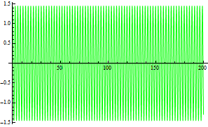
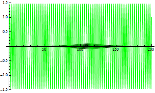
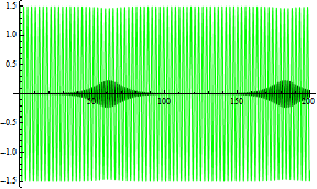
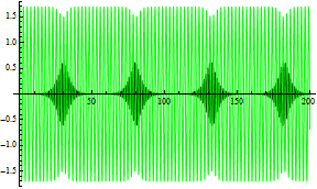
Figure 1: For $t\in[0,200]$ (left to right, top to bottom): the solutions $y_{1}$ (green) and $z_{1}$ (black) of (7)-(12) for $\|y_{1}\|_{\infty}=1.45,\,1.47,\,1.5,\,1.7$.

For $\|y_{1}\|_{\infty}=1.45$ no wide torsion appears, which means that the solution $(y_{1},0)$ is torsionally stable. For $\|y_{1}\|_{\infty}=1.47$ we see a sudden increase of the torsional oscillation around $t\approx 50$. Therefore, the stability threshold for the vertical amplitude of oscillation lies in the interval $[1.45,1.47]$. Finer experiments show that the threshold is $\|y_{1}\|_{\infty}\approx 1.46$, corresponding to a critical energy of about $E\approx 4.9$. For increasing $\|y_{1}\|_{\infty}$ the phenomenon is anticipated in time and amplified in magnitude.

3 How to introduce the aerodynamic forces into the model?

Even in absence of wind, an aerodynamic force is exerted on the bridge by the surrounding air in which the structure is immersed, and is due to the relative motion between the bridge and the air. Pugsley [14, $\S$ 12.7] assumes that the aerodynamic forces depend linearly on the “cross” derivatives and functions. Similarly, Scanlan-Tomko [15] obtain the following equations satisfied by the torsional angle $\theta$:

$$I\,[\ddot{\theta}(t)+2\zeta_{\theta}\omega_{\theta}\dot{\theta}(t)+\omega_{\theta}^{2}\theta(t)]=A\dot{\theta}(t)+B\theta(t)\ ,$$ (13)

where $I$, $\zeta_{\theta}$, $\omega_{\theta}$ are, respectively, associated inertia, damping ratio, and natural frequency. The r.h.s. of (13) represent the aerodynamic force which is postulated to depend linearly on both $\dot{\theta}$ and $\theta$ with $A,B>0$ depending on the structural parameters of the bridge. Let us mention that the arguments used in [15] to reach the l.h.s. of (13) have been the object of severe criticisms (see [10]), due to some rough approximations and questionable arguments. Nevertheless, the r.h.s. of (13) is nowadays recognized as a satisfactory description of aerodynamic forces.

Following these suggestions, we insert the aerodynamic forces in the 1-mode system (7). We first consider the case where only the cross-derivatives are involved. This leads to the following modified system:

$$\left\{\begin{array}[]{ll}\ddot{y}_{1}+3y_{1}+\frac{3}{2}y_{1}^{3}+\frac{9}{2}y_{1}z_{1}^{2}+\delta\dot{z}_{1}=0\\ \ddot{z}_{1}+7z_{1}+\frac{9}{2}z_{1}^{3}+\frac{27}{2}z_{1}y_{1}^{2}+\delta\dot{y}_{1}=0\end{array}\right.$$ (14)

with $\delta>0$. As in (12), we take the initial conditions

$$y_{1}(0)=\sigma=10^{4}z_{1}(0)\,,\quad\dot{y}_{1}(0)=\dot{z}_{1}(0)=0$$ (15)

for different values of $\sigma$ and we wish to highlight the differences, if any, between (7) and (14). For (14) we have no energy conservation; however, let us consider the (variable) energy function

$$E(t)=\frac{\dot{y}_{1}^{2}}{2}+\frac{\dot{z}_{1}^{2}}{6}+\frac{3}{2}y_{1}^{2}+\frac{7}{6}z_{1}^{2}+\frac{9}{4}y_{1}^{2}z_{1}^{2}+\frac{3}{8}(y_{1}^{4}+z_{1}^{4})\,.$$ (16)

Let us now consider the case where also the cross-terms of order 0 are involved. Then, instead of (14) we obtain the system

$$\left\{\begin{array}[]{ll}\ddot{y}_{1}+3y_{1}+\frac{3}{2}y_{1}^{3}+\frac{9}{2}y_{1}z_{1}^{2}+\delta(\dot{z}_{1}+z_{1})=0\\ \ddot{z}_{1}+7z_{1}+\frac{9}{2}z_{1}^{3}+\frac{27}{2}z_{1}y_{1}^{2}+3\delta(\dot{y}_{1}+y_{1})=0\end{array}\right.$$ (17)

where the coefficient 3 in the second equation comes from the variation of the energy

$$E(t)=\frac{\dot{y}_{1}^{2}}{2}+\frac{\dot{z}_{1}^{2}}{6}+\frac{3}{2}y_{1}^{2}+\frac{7}{6}z_{1}^{2}+\frac{9}{4}y_{1}^{2}z_{1}^{2}+\frac{3}{8}(y_{1}^{4}+z_{1}^{4})+\delta y_{1}z_{1}\,.$$ (18)

Also for (17) we do not have energy conservation but the function $E$ in (18) better approximates the internal energy. It may be questionable whether to include the last term $\delta y_{1}z_{1}$ into $E$ since this term depends on the aerodynamic forces. However, the behavior of $E$, which we analyze in the next section, does not depend on the presence of this term.

4 Numerical results

For (14) we first take $\sigma=1.47$ and we modify the aerodynamic parameter $\delta$. To motivate this choice we note that no energy transfer seems to occur for $\sigma$ below this threshold, furthermore $\sigma=1.47$ is also the numerical threshold found when no aereodynamic force is inserted in the model, see Section 2. In Figures 2 and 3 we plot both the behavior of the solutions (first line) and the behavior of the energy $E(t)$ (second line), for increasing values of $\delta$.

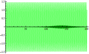
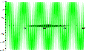
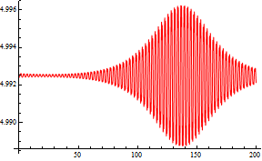
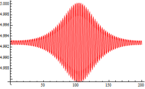
Figure 2: For $t\in[0,200]$: the solutions $y_{1}$ (green) and $z_{1}$ (black) of (14)-(15) for $\sigma=1.47$ and $\delta=0.01,\,0.02$ (left to right, first line). Second line (red): the energy $E=E(t)$ defined in (16).

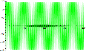
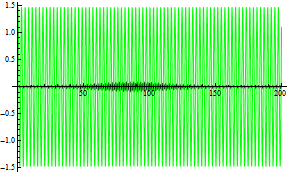
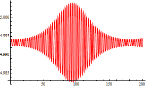
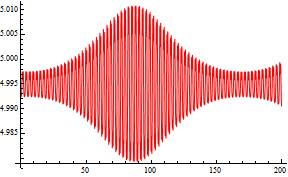
Figure 3: For $t\in[0,200]$: the solutions $y_{1}$ (green) and $z_{1}$ (black) of (14)-(15) for $\sigma=1.47$ and $\delta=0.03,\,0.05$ (left to right, first line). Second line (red): the energy $E=E(t)$ defined in (16).

The first lines in Figures 2 and 3 should be compared with the second picture in Figure 1 (case $\delta=0$). We note that, as the aerodynamic parameter increases, the transfer of energy is anticipated but it is not amplified. Quite surprisingly, on the second line we see that the energy $E(t)$ remains almost constant except in the interval of time where the transfer of energy occurs: for increasing aerodynamic parameters $\delta$ we observe increasing variations in the energy behavior.

Then we maintain fixed $\delta=0.01$ and we increase the initial energy, that is, the initial amplitude of oscillation. In Figures 4 and 5 we plot both the behavior of the solutions (first line) and the behavior of the energy $E(t)$ (second line), for increasing values of $\sigma$.

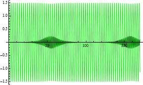
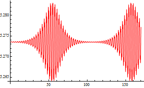
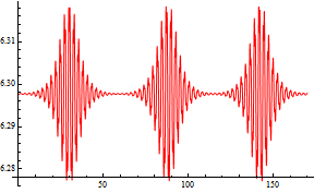
Figure 4: For $t\in[0,170]$: the solutions $y_{1}$ (green) and $z_{1}$ (black) of (14)-(15) for $\delta=0.01$ and $\sigma=1.5,\,1.6$ (left to right, first line). Second line (red): the energy $E=E(t)$ defined in (16).

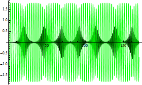
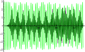
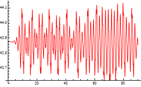
Figure 5: For $t\in[0,170]$: the solutions $y_{1}$ (green) and $z_{1}$ (black) of (14)-(15) for $\delta=0.01$ and $\sigma=1.8,\,3$ (left to right, first line). Second line (red): the energy $E=E(t)$ defined in (16).

It turns out that all the phenomena are anticipated (in time) and amplified (in width) and reach a quite chaotic behavior for $\sigma=3$ where we had to stop the numerical integration at $t=90$.

For (17) we take again as initial conditions (15) but with $\sigma\geq 1.47$ so that we are above the energy threshold of instability, see Section 2. In Figure 6 we plot both the behavior of the solution (first line) and the behavior of the energy $E(t)$ (second line) of (17)-(15).

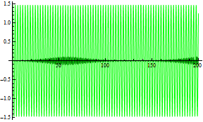
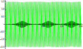
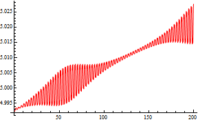
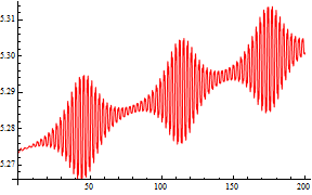
Figure 6: For $t\in[0,200]$: the solutions $y_{1}$ (green) and $z_{1}$ (black) of (17)-(15) for $\delta=0.01$ and $\sigma=1.47,\ 1.5$ (left to right, first line). Second line (red): the energy $E=E(t)$ defined in (18).

It is quite visible that the instability is further anticipated but now also the amplitude is enlarged. Moreover, the energy increases also in absence of torsional instability: this variation is due to the cross-derivatives since all the other terms appear in the energy (18). The very same behavior is obtained for the internal energy, namely the energy (18) without the last term $\delta y_{1}z_{1}$. We also remark that the energy $E$ fails to follow a regular pattern only in presence of instability. We only quote these numerical results because all the other experiments gave completely similar responses.

5 Theoretical results

As pointed out by Irvine [8, p.176], the numerical approach is probably the most appropriate to analyze a model which also involves aerodynamic forces. The reason is that a satisfactory stability theory for systems such as (14) and (17) is not available. Nevertheless, some theoretical conclusions can be drawn also for these systems, in the spirit of the results obtained in [4] (see also Section 2), where the main idea is to study the solutions of the systems near the pure vertical mode $\bar{y}$. Here “pure” means that no interactions with the surrounding are admitted and only the structural behavior of the bridge is considered. Let us explain how some of the results for the isolated system (7) may be extended to (14); one can then proceed similarly for (17).

For system (7), two steps are necessary to define the torsional stability of the unique (periodic) solution $\bar{y}$ of (9) (the pure mode):

(i) we linearize the torsional equation of the system (7) around $(\bar{y},0)$, see (11);

(ii) we say that the pure vertical mode $\bar{y}$ at energy $E(\eta_{0},\eta_{1})$ is torsionally stable if the trivial solution of (11) is stable.

We point out that the system (7) is isolated and that (11) is unforced. In this situation, the above steps (i)-(ii) are equivalent to:

(I) in the torsional equation of the system (7) we drop all the $z_{1}$-terms of order greater than or equal to one and we replace $y_{1}$ with $\bar{y}$;

(II) we say that the pure vertical mode $\bar{y}$ at energy $E(\eta_{0},\eta_{1})$ is torsionally stable if all the solutions of (11) are globally bounded.

If we replace (7) with the system (14), then (i)-(ii) make no sense while (I)-(II) do. A linearization as in (i) would exclude the aerodynamic forces, while acting as in (I) preserves them and gives rise to the forced Hill equation

$$\ddot{\xi}+a(t)\xi=f(t)\quad\mbox{with}\quad a(t)=7+\frac{27}{2}\overline{y}(t)^{2}\text{ and }f(t)=-\delta\dot{\bar{y}}(t)\,,$$ (19)

where $\bar{y}$ is the unique periodic solution of (9). Needless to say, $f$ and $a$ have the same period. The definition (ii) is inapplicable to (19) since $\xi\equiv 0$ is not a solution, while (II) is a verifiable property for (19). This is the definition of stability that we adopt for the vertical mode $\bar{y}$ in presence of aerodynamic forces. With this definition we can prove the following statement.

Proposition 2.

Let $\overline{y}$ be the pure vertical mode at energy $E(\eta_{0},\eta_{1})$, that is, the solution of (9). Then $\bar{y}$ is torsionally stable for (7) if and only if it is torsionally stable for (14).

Proof. Assume that $\bar{y}$ is torsionally stable for (7), then the trivial solution of (11) is stable (condition (i)) or, equivalently, all the solutions of (11) are globally bounded (condition (II)). Let $T$ be the period of $a(t)$, from the classical Floquet theory any (stable) solution of (11) may be written as

$$\xi_{h}(t)=A\xi_{1}(t)+B\xi_{2}(t)=Ae^{i\beta_{1}t}\varphi_{1}(t)+Be^{i\beta_{2}t}\varphi_{2}(t)\,,$$ (20)

where $A,B\in\mathbb{R}$, $\beta_{1}\neq\beta_{2}$ are real numbers such that $e^{i\beta_{j}T}\neq\pm 1$ ($j=1,2$) and $\varphi_{1}$ and $\varphi_{2}$ are $T$-periodic functions. By the variation of constants formula we then find that any solution of (19) takes the form

$$\xi(t)=\xi_{h}(t)-\frac{1}{c^{2}}\Big{[}e^{i\beta_{1}t}\varphi_{1}(t)\int_{0}^{t}e^{i\beta_{2}s}\varphi_{2}(s)f(s)\,ds-e^{i\beta_{2}t}\varphi_{2}(t)\int_{0}^{t}e^{i\beta_{1}s}\varphi_{1}(s)f(s)\,ds\Big{]}$$

where $c^{2}$ is the (constant) Wronskian of $\xi_{1}$ and $\xi_{2}$, namely $c^{2}=\xi_{1}(t)\xi_{2}^{\prime}(t)-\xi_{2}(t)\xi_{1}^{\prime}(t)$. From [4, Formula (53)] we know that $|\dot{\bar{y}}(t)|\leq\sqrt{2E}$ for every $t>0$, hence $|f(t)|\leq\delta\sqrt{2E}$ for every $t>0$. This proves the boundedness of the general solution $\xi$ and, in turn, the torsional stability of $\bar{y}$ for (14).

Assume now that $\bar{y}$ is torsionally stable for (14). Then $\xi$ is bounded for any choice of $\xi_{h}$, that is, any choice of the constants $A$ and $B$ in (20). This shows that also $\xi_{h}$ is bounded and proves the stability of $\bar{y}$ for (7). $\Box$

This statement deserves a couple of straightforward comments.

$\bullet$ In agreement with the numerical results described in Section 4, Proposition 2 shows that the energy threshold for stability does not depend on the strength of the aerodynamic forces; in particular, an isolated system has the same energy threshold.

$\bullet$ By applying Propositions 1 and 2 we infer that the energy threshold for the stability of (14) is at least $\frac{235}{294}$.

6 Conclusions

It is clear that in absence of wind or external sources a bridge remains still. A vertical load, such as a vehicle, bends the bridge and creates a bending energy. Less obvious is the way the wind inserts energy into the bridge: let us outline how this happens. When a fluid hits a bluff body its flow is modified and goes around the body. Behind the body, or a “hidden part” of the body, the flow creates vortices which are, in general, asymmetric. This asymmetry generates a forcing lift which starts the vertical oscillations of the body. Up to some minor details, this explanation is shared by the whole community and it has been studied with great precision in wind tunnel tests, see e.g. [9, 16].

The vortices induced by the wind increase the internal energy of the structure by generating wide vertical oscillations. When the amount of energy reaches a critical threshold our results in [4] show that a structural instability appears: this is the onset of torsional oscillations. The results in the present paper show that, at this stage, the aerodynamic forces excite the internal energy irregularly giving rise to further self-excited oscillations.

The whole energy-oscillation mechanism is here described through a very simplified model which certainly needs to be significantly improved. But, at least qualitatively, we believe that the “true” mechanism in a suspension bridge will follow this pattern:

1) the interaction of the wind with the structure creates vortices;

2) vortices create a lift which starts vertical oscillations of the bridge;

3) when vertical oscillations are sufficiently large, torsional oscillations may appear;

4) the onset of torsional instability is of structural nature;

5) the aerodynamic forces excite the energy only when the structural torsional instability appears;

6) the energy threshold of stability is independent of the strength of aerodynamic forces.

References

- [1]
- [2] O.H. Ammann, T. von Kármán and G.B. Woodruff, The failure of the Tacoma Narrows Bridge, Federal Works Agency, Washington D.C., (1941).
- [3] G. Arioli and F. Gazzola, A new mathematical explanation of what triggered the catastrophic torsional mode of the Tacoma Narrows Bridge collapse, to appear in App. Math. Modelling.
- [4] E. Berchio and F. Gazzola, A qualitative explanation of the origin of torsional instability in suspension bridges, preprint, arXiv0967187.
- [5] K.Y. Billah and R.H. Scanlan, Resonance, Tacoma Narrows Bridge failure, and undergraduate physics textbooks, Amer. J. Physics, 59 (1991), 118-124.
- [6] G.W. Hill, On the part of the motion of the lunar perigee which is a function of the mean motions of the sun and the moon, Acta Math., 8 (1886), 1-36.
- [7] G. Holubová and A. Matas, Initial-boundary value problem for nonlinear string-beam system, J. Math. Anal. Appl., 288 (2003), 784-802.
- [8] H.M. Irvine, Cable Structures, MIT Press Series in Structural Mechanics, Massachusetts, 1981.
- [9] A. Larsen, Aerodynamics of the Tacoma Narrows Bridge - 60 years later, Struct. Eng. Internat., 4 (2000), 243-248.
- [10] P.J. McKenna, Oscillations in suspension bridges, vertical and torsional, Disc. Cont. Dynam. System S, 7 (2014), 785-791.
- [11] K.S. Moore, Large torsional oscillations in a suspension bridge: multiple periodic solutions to a nonlinear wave equation, SIAM J. Math. Anal., 33 (2002), 1411-1429.
- [12] B.G. Pittel and V.A. Yakubovich, A mathematical analysis of the stability of suspension bridges based on the example of the Tacoma Bridge (Russian), Vestnik Leningrad Univ., 24 (1969), 80-91.
- [13] R.H. Plaut and F.M. Davis, Sudden lateral asymmetry and torsional oscillations of section models of suspension bridges, J. Sound and Vibration, 307 (2007), 894-905.
- [14] A. Pugsley, The theory of suspension bridges, Edward Arnold, London, 1968.
- [15] R.H. Scanlan and J.J. Tomko, Airfoil and bridge deck flutter derivatives, J. Eng. Mech., 97 (1971), 1717-1737.
- [16] R. Scott, In the wake of Tacoma. Suspension bridges and the quest for aerodynamic stability, ASCE Press, 2001.
- [17] N.E. Zhukovskii, Finiteness conditions for integrals of the equation (Russian), Mat. Sb., 16 (1892), 582-591.
- [18]