A spring-block analogy for the dynamics of stock indexes
Abstract
A spring-block chain placed on a running conveyor belt is considered for modeling stylized facts observed in the dynamics of stock indexes. Individual stocks are modeled by the blocks, while the stock-stock correlations are introduced via simple elastic forces acting in the springs. The dragging effect of the moving belt corresponds to the expected economic growth. The spring-block system produces collective behavior and avalanche like phenomena, similar to the ones observed in stock markets. An artificial index is defined for the spring-block chain, and its dynamics is compared with the one measured for the Dow Jones Industrial Average. For certain parameter regions the model reproduces qualitatively well the dynamics of the logarithmic index, the logarithmic returns, the distribution of the logarithmic returns, the avalanche-size distribution and the distribution of the investment horizons. A noticeable success of the model is that it is able to account for the gain-loss asymmetry observed in the inverse statistics. Our approach has mainly a pedagogical value, bridging between a complex socio-economic phenomena and a basic (mechanical) model in physics.
keywords:
dynamics of stock indexes , spring-block models , stylized facts1 Introduction
Spring-block (SB) models have been used for a long time to model complex phenomena in physics and engineering. This model family was introduced by Burridge and Knopoff [1] for describing the distribution of earthquakes after their magnitudes. In its original version a one-dimensional chain of blocks connected by springs is placed on a moving plane. The blocks are free to slide on this plane, subject to a velocity dependent friction force. All blocks are connected with additional springs to a second plane, which is in rest, and it is placed above the spring-block chain. This system was meant to describe two tectonic plates that are in relative motion respective to each other, exhibiting a complex stick-slip dynamics. In such an approach the slipping motion of the blocks will lead to energy dissipation and the complex avalanche-like dynamics will yield a scale-free distribution for the energy dissipated in avalanches. The model exhibits a complex dynamics and Self-Organized Criticality (SOC) [2, 3].
This very simple physical system formed by an ensemble of blocks interconnected with springs and placed on a frictional surface resulted in many interesting applications. It was successful in reproducing desiccation patterns and dynamics of crack formation in mud, clay or thin layers of paint [4, 5], self-organized patterns in wetted nano-sphere [6] or nano-tube [7] arrays or even crack structures obtained in glass [8]. It was applied for describing the Portevin Le Chatelier effect [9] and magnetization phenomena in ferromagnets, including the Barkhausen noise [10]. Besides applications in physics, the spring-block model got some interdisciplinary applications as well. Formation of traffic jams in a single-lane highway traffic [11] or detection of region-like structures [12] in a delimited geographic space are a few recent applications in such sense. Continuing this line of studies, here we intend to consider a simple one-dimension spring-block chain for revealing a pedagogically useful and interesting analogy with the dynamics of stock indexes.
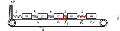
The simplest version of the model will be considered here, the one referred in the literature as ”train model” [13]. As it is sketched in Figure 1, a spring-block chain is placed on a running conveyor-belt, so that the first block is fixed with a spring to an external, static point. As a result of the dragging effect of the conveyor belt, the chain is stretched and a complex-stick slip dynamics emerges. Both the case of one block alone [14, 15, 16, 17, 18, 19] and the case of a chain formed by several blocks [14, 16, 20, 21, 22, 23, 24, 25] were considered in previous theoretical and experimental studies. Coexistence of chaotic dynamics and SOC was observed by many authors [14, 25]. Nonlinearity was introduced in the model via friction forces. Several friction force profiles were considered, starting from velocity-weakening friction forces combined with a constant static friction force [14, 22, 24] to simple state-dependent friction forces [18, 25]. Our aim here is rather different from these previous studies. Instead of mapping the dynamical complexity of such a system, we take a different turn and use the system as a simple analogy for modeling the dynamics of stock indexes.
The dynamics of stock indexes are in the focus of physicists from a quite long time [26]. The existence of many stylized facts in the financial market (see for example [26]) captured the interest of the statistical physics community. Many simple models have been used to reproduce statistical features of price/index fluctuations (for a review see for example [27]). Definitely, the most basic approach among them is the simple random walk (or Brownian dynamics) model applied to the logarithmic index [28]. This model is known as the geometric random walk model [29]. The fact that dynamics of stock prices can be approached by a simple geometric random walk is one of the most interesting empirical fact about financial markets . This simple model was first proposed by the French mathematician Louis Bachelier in the early 1900, and it has been strongly debated since then. The most important support for this model comes from the experimental fact that volatility of stock returns tend to be approximately constant in long term. Although this model cannot account of many important statistical aspects of the index or stock price fluctuations (such as time-varying volatility [30, 31], evidence of some positive autocorrelations [32], or the asymmetry of the investment horizons distribution for positive and negative return levels [33]), it’ s simplicity and intuitive nature makes it pedagogically useful. It can be considered as a first step (zero order model) towards understanding the nature of the stock index dynamics by a general model of mathematics and physics.
Similarly with random walk, the SB system is also a general model of physics, which is appropriate for capturing in an elegant manner universal trends in the dynamics of stock indexes. Although the physical picture behind the two phenomena (motion of a spring-block chain and the dynamics of stock indexes) is rather different, a simple and useful analogy can be drawn between them. This analogy might be useful for pedagogical reasons and for understanding some stylized facts. Our motivation here was not to give a model which performs better than the nowadays used rather complex approaches [34]. Instead of this we focus on the simplicity and visuality of the model, offering a pedagogical picture that is one step ahead of the basic random walk approach. The rest of the paper is about the proposed analogy between the dynamics of stock indexes and the simple spring-block chain system, and also about discussing the modeling power of such an approach.
2 Stylized facts for the dynamics of stock indexes
The performance of stocks and markets, and thus the performance of the economy of a region or state, over a certain time history is traditionally measured by the distribution of the logarithmic return [33], which gives the generated return over a certain time period. For stock market indexes it is defined as the natural logarithm of the price change over a fixed time interval:
| (1) |
where is the logarithmic index ( is the value of the index or the price of a stock). The logarithmic return indicates, how much the logarithmic index or stock prices have increased or decreased in a fixed time interval, thus presents the economical performance of a company. Among others, the advantage of using logarithmic returns is, that it is an additive quantity.
The financial time series considered as example in the followings is the Dow Jones Industrial Average (DJIA) index. We deal with the daily closure prices for about an 80 year long time period (more than 20000 trading days), from 1.10.1928. to 1.02.2011. We have chosen the DJIA index, because this is the oldest continuously functioning index and it can be freely downloaded from the internet. It is an index that shows how 30 large publicly owned companies (like General Electric, IBM, Microsoft, McDonald’s, Coca-Cola, etc.) based in the United States have traded during a standard trading session in the stock market. The value of the DJIA index can be calculated quite simply, though is not the actual average of the prices of its component stocks, but rather the sum of the component prices divided by a divisor, which changes whenever one of the component stocks has a stock split or stock dividend, so as to generate a consistent value for the index [35].
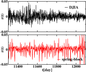
As an example in Fig. 2. the time series of daily returns for DJIA are shown (this means we consider day long time intervals).
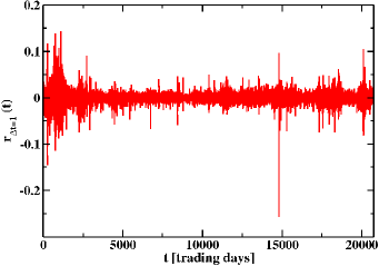
The standard deviation of daily log-returns is called volatility. The volatility is a measure for the variation of price of a financial instrument (e.q. stocks), therefore in the case of higher volatilities there is a higher probability of large price fluctuations, thus for large gains or losses. For the DJIA index, the historical volatility of the daily log-returns is about , i.e. .
The distribution of logarithmic returns measure how much an initial investment, made at time , has gained or lost by the time . Empirical results have demonstrated, that the distribution of returns can be approximated by a Gaussian distribution, although there are meaningful differences, such as the presence of fat tails [26, 28, 33, 36]. The fat tails correspond to a much larger probability for large price changes than what to be expected from a Gaussian statistics, an assumption made in the mainstream theoretical finance [26, 28, 37].
The method of inverse statistics in economics was recently suggested by Simonsen et al. [33], being inspired by earlier works in turbulence [38]. The method was adopted as an alternative measure of the financial market performance. The idea is to turn the problem around and ask the inverse question: what is the typical waiting time to generate a fluctuation of a given size in the price [33]? For this we have to determine for an index or a stock the distribution of time intervals needed to obtain a predefined return level. We search thus for the shortest interval, for which it is true, that:
| (2) |
or
| (3) |
Practically if given a fixed logarithmic return barrier (proposed by the investor) of a stock or an index, as well as a fixed investment date (when the investor buys some assets), the corresponding time span is estimated for which the log-return of the stock or index for the first time reaches the level . This is also called first passage time through the level [33]. In a mathematical formulation (for ) this is equivalent with:
| (4) |
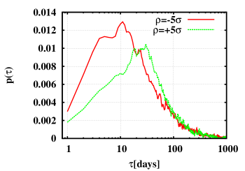
In the literature this time is termed as the investment horizon for the proposed log-return for that stock or index [33]. The investment horizon indicates for an investor the time interval he has to wait, if the investment was made at time , to achieve the proposed (e.q. ) log-return at . The normalized histogram of the accumulated values of the first passage times form the probability distribution function of the investment horizons. The method described above is called the method of inverse statistics. The distribution of investment horizons for the DJIA index is presented in Fig. 3. The maximum of the distribution function determines the most probable waiting time for that log-return, or in other words the most probable investment horizon. This is the optimal investment horizon for that stock or index. The first passage distribution gives also information about the stochasticity of the underlying asset price [39, 38].
Building up the inverse statistics of DJIA index also for negative return levels (i.e. ), it was found [37, 40] that the distribution of investment horizons is similar to the one for positive levels (with a pronounced maximum), though there is one important difference. For negative return levels the maximum of the probability distribution function is shifted to left, generating about a trading days difference in the optimal investment horizons. In Fig. 3 this asymmetry of the inverse statistics is presented for and log-returns. Later it was found, that the asymmetry of inverse statistics is present for every important stock index, thus stock markets present a universal feature, called the gain-loss asymmetry [37]. In contrary with the indexes, stock prices show a smaller degree of asymmetry [41, 42].
Minimal models have been proposed for explaining this apparent paradox. One of these models is termed the fear-factor model [43, 40]. In this model a synchronization-like concept is introduced, the so-called fear factor. The presence of this fear factor at certain times causes the stocks to all move downward, while at other times they move independently from each other. In this way the fear-factor model assumes stronger stock-stock correlations during dropping markets than during market raises [42]. Recently the idea of fear factor model was generalized by allowing longer time periods of stock-stock correlations [41]. Balogh et. al. [42] have demonstrated by conducting a set of statistical investigations on the DJIA index and its constituting stocks, that indeed there is stronger stock-stock correlation during falling markets. This empirical result gives confidence in the fear factor hypothesis.
3 The spring-block analogy
We consider the simple one dimensional SB system sketched in Fig. 1, referred in the literature as “train model” [13]. A spring-block chain, composed of identical blocks, is placed on a platform (conveyor belt) that moves with constant velocity. The first block is connected by a spring to a static external point. As a result, due to the dragging effect of the moving platform, the blocks will undergo a complex stick-slip dynamics [25].
As the conveyor belt is started with velocity, the whole system moves together with the belt until the first block starts to slip. The slipping moment occurs when the sum of elastic forces acting on a block overcomes the maximal value of the static friction force (). The slipping motion is tempered by the dynamical friction forces. The block sticks again to the belt when its relative velocity becomes zero. After that the process may start again (a movie about the dynamics in the spring-block system can be consulted at [48]).
In the analogy taken here, the price of individual stocks can be modeled as the positions of blocks, measured from an external static point. For example, if we would like to use this analogy for the DJIA index that represents the economical state of 30 large American stocks, a chain composed of blocks will be considered in the model. As one can set up a ranking between the stocks as a function of their price in the index, the pre-existing order between the blocks of the chain is not completely irrelevant. Of course, the ranking of stocks by prices can change throughout the time. The corresponding event would be, that blocks come through each other, but this unphysical phenomena is not considered in this simple model.
In the framework of our model the value of the index is defined as the center of mass of the system, measured in the static coordinate system:
| (5) |
The elastic forces acting between blocks via springs correspond to stock-stock correlations. The conveyor belt acts on the system through the friction forces. The pulling imposed by the belt models the desire for grow, a general trend expected from all companies and societies. For small belt velocities the stick-slip dynamics, will lead to ”avalanches” of different sizes. Therefore, the length of the chain, defined by the position of the last block fluctuates as a function of time with largely varying amplitudes, as shown in Fig. 8.a. in Ref. [25]. This self organized behavior leads to abrupt drops in the value of the index, when all the stock prices fall in a correlated manner [42].
In order to account for the random jumps of the index when it is raising continuously and also for the observed fat-tail distribution of the positive logarithmic returns the velocity of the belt is randomly varied (more details in Appendix A).
An important ingredient for making the proposed analogy to work is to choose the sampling time in the dynamics of . The financial time series (the DJIA index in our case) represents the daily closure prices for about an 80 year-long time period. Similarly with many other studies in the literature, intra-day variability of the index was not considered in this study. In the spring-block analogy we need thus to define also a discrete time-step, beside the obvious continuous time of the dynamics. For this, the time-series of the simulation needs to be sampled with a well defined frequency, producing in such manner a discrete time-series that should correspond to a one trading day time-interval. This sampling frequency will influence the volatility measured in the artificial index generated by the spring-block model. Since the volatility of log-returns for the DJIA index is known we can fix the sampling interval in the model by imposing this experimental value (see Appendix A).
The power of the analogy introduced in this model consist in the fact that the dynamics shows many similarities with the observed dynamics of stock indexes. Details for the dynamics, computer simulations and the used parameters for the spring-block chain are given in Appendix A.
4 Model results in comparison with historical stock market data
Considering the simulation parameters specified in Appendix A and the integration method describer in Appendix B, we compare now the statistical results offered by the SB train model and those measured from the DJIA index. The parameter values were chosen for reproducing in an optimal manner all the stylized facts measured for the DJIA. One can of course choose other parameters that will lead to better results for some of the statistical measures, but in such cases larger differences will be obtained for the others. We recall however that our stated aim here was not to give a realistic description for the dynamics of stock indexes, and it is not surprising thus that with such a simple mechanical analogy one cannot reproduce all the observed statistical features for the dynamics of stock indexes.
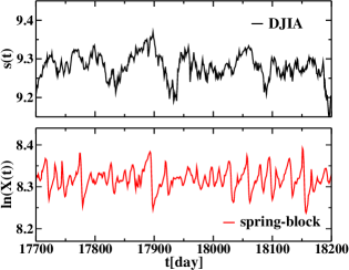
In Figure 4 we show a first visual comparison between the logarithmic index for the DJIA () and the one generated by the SB model (). In spite of the fact that one can observe visually detectable statistical differences, the results are quite promising. Similar results can be concluded if we analyze the logarithmic returns for day (Figure 5).
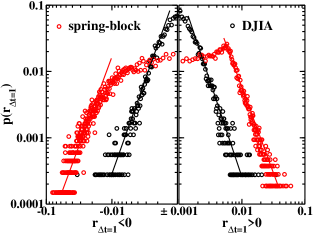
The differences and similarities detected by the visual examination of the logarithmic returns are better illustrated if we plot the distribution function of the logarithmic index (Figure 6). From the log-log plot one will conclude that the power-law tails observed for high return values are successfully reproduced by the SB model with the chosen random driving of the conveyor belt. There are however significant differences in the low returns limit. Seemingly the distribution function for the DJIA is more narrow and less asymmetric than the one obtained in our SB approach.
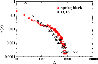
For further statistical comparison one can construct the avalanche-size distribution for both the DJIA and the SB model. An avalanche is defined as a consecutive, monotonic drop in the index, between time moment and . The distribution of the variation in the index for the avalanches ( for the DJIA and for the SB model) generates the avalanche-size distribution. Measured results are compared in Figure 7. As it is expectable in both systems there are many small avalanches and one will find also a few extremely large ones. This situation is characteristic for self-organized criticality, a feature that seemingly both system exhibit. The two distribution functions are rather similar, although the trend for the SB model is more complex than the one obtained for the case of the DJIA.
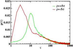
Finally we consider the inverse statistics, i.e. the distribution of the investment horizons for a fixed logarithmic return value. We considered the same and log-return values as in the case of the DJIA index (Figure 3) and the results obtained for the SB model are plotted in Figure 8. The SB model reproduces with success the gain-loss asymmetry observed in real stock index data. Although the position of the maximum for the curves is shifted by a few days, the shape of the curves and asymmetries in the investment horizons are similar. The SB model is capable thus for reveling also this subtle statistical feature characteristic for stock indexes.
5 Conclusions
A simple mechanical analogy has been considered for modeling the dynamical features of stock indexes. A chain of blocks connected by springs subjected to the continuous driving of a running conveyor belt was used as a model system for stock indexes. Contrarily with the large number of recently reported models, here our aim was rather different. Instead of considering an economically relevant and complex description, we tested the applicability of a general and simple model of physics: the spring-block system. The analogy we have made is well motivated and highlights the connections among individual stocks prices and their collective behavior. We have fixed the driving (speed of the conveyor belt) and the free parameters of the model so that most of the stylized facts known for the DJIA stock index are reasonable well reproduced. When judging the success or fail of our approach one has to take into account also the fact, that we did not focused only on a few and selected stylized facts, as most of the models proposed in the recent literature does. Instead, we considered all the used and measurable statistical features of the DJIA stock index, trying to reproduce them as a whole with a fixed parameter set. An important results of the introduced model is that it accounts for the puzzling phenomenon of gain-loss asymmetry which is observed in the inverse statics, and the model describes also well the avalanche-size distribution curves. In spite of the success in reproducing qualitatively the known statistical features of the index dynamics, a finer statistics revealed noticeable differences. We consider this normal, since one cannot expect from a such a simple mechanical analogy a deeper understanding for a complex socio-economic phenomenon.
In conclusion, we believe that the model introduced here has mainly a pedagogical value for the interdisciplinary field of econophysics. It offers an appealing mechanical analogy for physicist to approach collective phenomena in stock markets.
Acknowledgments
This research was supported by the European Union and the State of Hungary, co-financed by the European Social Fund in the framework of TÁMOP 4.2.4.A/2-11-1-2012-0001 ‘National Excellence Program’.
Appendix A. Details of the dynamics for the spring-block system
We consider a chain formed by identical blocks of mass . The blocks are connected by identical springs of linear spring constant and undeformed length . The challenge in computer modeling is the quantification of the friction and spring forces and the numerical integration of the equations of motion. Dimensionless units are used so that , , and . The value for was chosen for the sake of an easier graphical visualization (spring length corresponding to pixels). In order to have these dimensionless values to correspond to a realistic experimental situation, the units are chosen as: kg for mass, N/m for spring constant, and m for length. The units of the other quantities follow from dimensional considerations. The time, velocity and force units are thus, s, m/s, and N, respectively.
The equation of motion for the -th block of the chain is
| (6) |
where and , respectively, and is the relative velocity of the block to the conveyor belt. The elastic force, , and the friction force, , are defined below. The numerical method used for integrating the equations of motions are presented in Appendix B, and the time-step was chosen as time units.
The elastic force in the springs is linear, up to a certain deformation value, . For higher deformations, this dependence is assumed to become exponential, with an exponent bigger (in modulus) for negative deformations (see Fig. 9). Accordingly,
| (7) |
where we have chosen , for and for . With these choices the model is quite realistic for an experimental realization (see for example [25]) since the nonlinearity of spring forces is taken into account and collisions between blocks are avoided. At the same time the choice of parameters and is somewhat ad-hoc and we have not carried out a systematic change of them.

For the velocity dependent friction the simple Coulomb’s law of friction is used. Both the static and kinetic friction forces are independent of velocity modulus. A block remains in the stick state until the resultant external force exceed the value of the static friction force, . For higher external force values the block starts to slide in the presence of the kinetic friction force . We assume that, the ratio of the static and kinetic friction forces is constant. The friction force acting on the block depends both on , where is the signum function and is the block’s speed relative to the conveyor belt, and on the value of the resultant external forces acting on it. In our 1D setup, the friction force orientation is given only by its sign:
| (8) |
where and is the velocity of the block relative to the laboratory frame. In order to use the same friction force value as in our previous experiments [25], in the dimensionless units the static friction force is taken as and we considered .
For reproducing also the empirically measured fat-tail (power law) distribution of the logarithmic returns, the speed of the conveyor belt was varied randomly with a power law distribution, normalized in the velocity interval. The exponent of the power function was chosen to be . In such way the model reproduces the empirically measured power law distributions for positive and also for negative returns [47].
Assuming that the daily volatility of the logarithmic returns for DJIA and the one given by our model should be the same, we determined the sampling time for the dynamics of . In the units of our simulations, we obtained (500 integration steps). With this sampling frequency the volatility of log-returns for the artificial index turns to be , which corresponds to the empirical value up to three decimals.
Appendix B - numerical integration of the equation of motions
We briefly describe here the method used to integrate the equations of motion (6) and to handle the discontinuous stick-slip dynamics of the blocks. When a block is stuck to the conveyor belt, it moves together with it at constant velocity . Therefore, the position of the th block relative to the ground is calculated with the simple
| (9) |
equation. When a block is slipping relative to the belt, the basic Verlet method
| (10) |
is used to update its position. As can be seen, this is a third order method, which can be extended also to the velocity space as:
| (11) |
The instance when the th block sticks to the belt is found when the relative velocity changes its sign, while a block starts to slip when the sum of external forces acting on it exceed the maximal value of static friction forces, i.e. when . A more complicated stochastic numerical method was also developed to handle the stick-slip dynamics, but was found not to significantly alter the presented results [25].
References
- [1] R. Burridge and L. Knopoff, Bull. Seism. Soc. Am, vol. 57, 341–371 (1967).
- [2] P. Bak, C. Tang, and K. Wiesenfeld, Phys. Rev. Lett. 59, 381 (1987).
- [3] J. M. Carlson and J. S. Langer, Phys. Rev. A 40, 6470 (1989).
- [4] J. V. Andersen, Phys. Rev. B 49, 9981 (1994).
- [5] K. T. Leung and Z. Neda, Phys. Rev. Lett. 85, 662 (2000).
- [6] F. Jarai-Szabo, S. Astilean, and Z. Neda, Chem. Phys. Lett. 408, 241 (2005).
- [7] F. Jarai-Szabo, E.-A. Horvat, R. Vajtai, and Z. Neda, Chem. Phys. Lett. 511, 378 (2011).
- [8] E.-A. Horvat, F. Jarai-Szabo, Y. Brechet, and Z. Neda, Cent. Eur. J. Phys. 10, 926 (2012).
- [9] M. A. Lebyodkin, Y. Brechet, Y. Estrin, and L. P. Kubin, Phys. Rev. Lett. 74, 4758 (1995).
- [10] K. Kovacs, Y. Brechet, and Z. Neda, Model. Simul. Mater. Sc. 13, 1341 (2005).
- [11] F. Jarai-Szabo and Z. Neda, Physica A 391, 5727 (2012).
- [12] G. Mate, Z. Neda and J. Benedek, PLOS ONE, vol. 6, e16518 (2011)
- [13] M. de Sousa Vieira, Phys. Rev. A 46, 6288 (1992).
- [14] M. de Sousa Vieira and H. J. Herrmann, Phys. Rev. E 49, 4534 (1994).
- [15] T. Baumberger, C. Caroli, B. Perrin, and O. Ronsin, Phys. Rev. E 51, 4005 (1995).
- [16] G. L. Vasconcelos, Phys. Rev. Lett. 76, 4865 (1996).
- [17] F.-J. Elmer, J. Phys. A - Math. Gen. 30, 6057 (1997).
- [18] H. Sakaguchi, J. Phys. Soc. Jpn. 72, 69 (2003).
- [19] A. Johansen, P. Dimon, C. Ellegaard, J. S. Larsen, and H. H. Rugh, Phys. Rev. E 48, 4779 (1993).
- [20] M. de Sousa Vieira and A. J. Lichtenberg, Phys. Rev. E 53, 1441 (1996).
- [21] C. V. Chianca, J. S. Sa Martins, and P. M. C. de Oliveira, Eur. Phys. J. B 68, 549 (2009).
- [22] M. de Sousa Vieira, Phys. Lett. A 198, 407 (1995).
- [23] J. Szkutnik and K. Kulakowski, Int. J. Mod. Phys. C 13, 41 (2002).
- [24] B. Erickson, B. Birnir, and D. Lavallee, Nonlinear Proc. Geoph. 15, 1 (2008).
- [25] B. Sandor, F. Jarai-Szabo, T. Tel, and Z. Neda, Phys. Rev. E 87, 042920 (2013).
- [26] R. Mantegna and H.E. Stanley, An Introduction to Econophysics, Correlations and Complexity in Finance (Cambridge University Press, Cambridge, 2000)
- [27] S. Sinha, A. Chatterjee, A. Chackraborti,B.K. Chakrabarti, Econophysics (An Introduction), (Willey-WCH Verlag GmbH & Co KGaA, Weinhelm, 2011)
- [28] J. P. Bouchaud and M. Potters, Theory of Financial Risks (Cambridge University Press, Cambridge, UK, 2000)
- [29] B. G. Malkiel, Random Walk Down Wall Street (W.W. Norton & Company Inc., New York, 2007)
- [30] G. W. Schwert, The Journal of Finance, vol. XLIV, 1115 (1989)
- [31] F. Patzelt and K. Pawelzik, Scientific Reports, vol. 3, 2784 (2013)
- [32] T. Iwaisako, H. Daigaku, K. Kenkyujo, Stock index autocorrelation and cross-autocorrelations of size-sorted portfolios in the Japanese market ( Institute of Economic Research, Hitotsubashi University, Japan, 2007. )
- [33] I. Simonsen, M. H. Jensen, and A. Johansen, Eur. Phys. J. B vol. 27, 583 (2002).
- [34] F. Comte and E. Renault, Journal of Econometrics, vol. 73, 101–149, 1996.
- [35] A. Sullivan and S. M. Sherin, Economics: Principles in action (Upper Saddle River, New Jersey, 2003).
- [36] R. N. Mantegna and H. E. Stanley, Nature vol. 367, 46 (1995).
- [37] M. H. Jensen, A. Johansen, and I. Simonsen, Physica A, vol. 324, 338 (2003).
- [38] M. H. Jensen, Phys. Rev. Lett. vol. 83, 76 (1999).
- [39] L. Biferale, M. Cencini, D. Vergni, and A. Vulpiani, Phys. Rev. E vol. 60, R6295 (1999).
- [40] I. Simonsen, P. T. H. Ahlgren, M. H. Jensen, R. Donangelo, and K. Sneppen, Eur. Phys. J. B vol. 57, 153 (2007).
- [41] L. J. Siven, J. and J. L. Hansen, J. Stat. Mech.: Theory Exp. , P02004 (2009).
- [42] E. Balogh, I. Simonsen, B. Z. Nagy, and Z. Neda, Phys. Rev. E vol. 82, 066113 (2010).
- [43] R. Donangelo, M. H. Jensen, I. Simonsen, and K. Sneppen, J. Stat. Mech: Theo. Exp. , L11001 (2006).
- [44] J. Bouchaud, A. Matacz, and M. Potters, Phys. Rev. Lett vol. 87, 228701 (2001).
- [45] P. T. H. Ahlgren, M. H. Jensen, I. Simonsen, R. Donangelo, and K. Sneppen, Physica A 383, 1 (2007).
- [46] J. Lagger, Gain/loss Asymmetry and the Leverage Effect, Master’s thesis, Department of Management, Technology & Economics - ETH Zurich (2012).
- [47] A. Chakraborti, I. M. Toke, M. Patriarca, and F. Abergel, Quantitative Finance 11, 991 (2011).
- [48] The spring-block train model in action. movie on YouTube: https://www.youtube.com/watch?v=ObqeSR3PZd0&feature=youtu.be