Resummed Quantum Gravity Prediction for the Cosmological Constant and Constraints on SUSY GUTS

Abstract

We use our resummed quantum gravity approach to Einstein’s general theory of relativity in the context of the Planck scale cosmology formulation of Bonanno and Reuter to estimate the value of the cosmological constant as $\rho_{\Lambda}=(0.0024eV)^{4}$. We show that the closeness of this estimate to experiment constrains susy GUT models. We also address various consistency checks on the calculation.

Nuclear Physics B Proceedings Supplement nuphbp Nuclear Physics B Proceedings Supplement

BU-HEPP-14-06, Aug., 2014

1 Introduction

Weinberg’s suggestion [1] that the general theory of relativity may be asymptotically safe, with an S-matrix that depends on only a finite number of observable parameters, due to the presence of a non-trivial UV fixed point, with a finite dimensional critical surface in the UV limit, has received significant support from the calculations in Refs. [2, 3, 4, 5, 6, 7]. Using Wilsonian [8] field-space exact renormalization group methods, the latter authors obtain results which support Weinberg’s suggestion for the Einstein-Hilbert theory. Independently, we have shown [9, 10, 11, 12] that the extension of the amplitude-based, exact resummation theory of Ref. [13, 14] to the Einstein-Hilbert theory leads to UV-fixed-point behavior for the dimensionless gravitational and cosmological constants. We have called the attendant resummed (UV-finite) theory resummed quantum gravity. Causal dynamical triangulated lattice methods have been used in Ref. [15] also to show more evidence for Weinberg’s asymptotic safety behavior.

The results in Refs. [2, 3, 4, 5, 6, 7], while quite impressive, involve cut-offs and some dependence on gauge parameters which remain to varying degrees even for products such as that for the UV limits of the dimensionless gravitational and cosmological constants. Thus, we refer to the approach in Refs. [2, 3, 4, 5, 6, 7] as the ’phenomenological’ asymptotic safety approach. The noted dependencies are mild enough that the non-Gaussian UV fixed point found in these latter references is probably a physical result. But, the result cannot be considered final until it is corroborated by a rigorously cut-off independent and gauge invariant calculation, such as we have done in resummed quantum gravity. As the results from Refs. [15] involve lattice constant-type artifact issues, they too need to be corroborated by a rigorous calculation without such issues to be considered final. Resummed quantum gravity again offers an answer. The stage is thus prepared for us to try to make contact with experiment, as we do in what follows.

More specifically, the attendant approach in Refs. [2, 3, 4, 5, 6, 7] to quantum gravity has been applied in Refs. [17, 18] to provide an inflatonless realization of the successful inflationary model [20, 21] of cosmology : the standard Friedmann-Walker-Robertson classical descriptions are joined smoothly onto Planck scale cosmology developed from the attendant UV fixed point solution. A quantum mechanical solution is thus obtained to the horizon, flatness, entropy and scale free spectrum problems. Using the new resummed quantum gravity theory [9, 10, 11], the properties as used in Refs. [17, 18] for the UV fixed point of quantum gravity are reproduced in Ref. [12] with the “first principles” predictions for the fixed point values of the respective dimensionless gravitational and cosmological constants. In what follows, the analysis in Ref. [12] is carried forward [22] to an estimate for the observed cosmological constant $\Lambda$ in the context of the Planck scale cosmology of Refs. [17, 18]. We comment on the reliability of the result, as the estimate will be seen already to be relatively close to the observed value [23, 24]. The closeness to the observed value of our estimate allows us to constrain SUSY GUT models when this closeness is put on a more firm basis [25]. The closeness of our estimate to the experimental value again gives, at the least, some more credibility to the new resummed theory as well as to the methods in Refs. [2, 3, 4, 5, 6, 7, 15].

We present the discussion as follows. Section 2 gives a brief review of the Planck scale cosmology presented phenomenologically in Refs. [17, 18]. Our results in Ref. [12] for the dimensionless gravitational and cosmological constants at the UV fixed point are reviewed in Section 3. In Section 4, we use our results in Section 3 in the context of the Planck scale cosmology scenario in Refs. [17, 18] to estimate the observed value of the cosmological constant $\Lambda$ and we use the attendant estimate to constrain SUSY GUTs. We also address consistency checks on the analysis.

2 Planck Scale Cosmology

We begin withl the Einstein-Hilbert theory

$${\cal L}(x)=\frac{1}{2\kappa^{2}}\sqrt{-g}\left(R-2\Lambda\right).$$ (1)

Here, $R$ is the curvature scalar, $g$ is the determinant of the metric of space-time $g_{\mu\nu}$, $\Lambda$ is the cosmological constant and $\kappa=\sqrt{8\pi G_{N}}$ for Newton’s constant $G_{N}$. Using the phenomenological exact renormalization group for the Wilsonian [8] coarse grained effective average action in field space, the authors in Ref. [17, 18] have argued that the attendant running Newton constant $G_{N}(k)$ and running cosmological constant $\Lambda(k)$ approach UV fixed points as $k$ goes to infinity in the deep Euclidean regime. This means that $k^{2}G_{N}(k)\rightarrow g_{*},\;\Lambda(k)\rightarrow\lambda_{*}k^{2}$ for $k\rightarrow\infty$ in the Euclidean regime.

To make contact with cosmology, one may use a connection between the momentum scale $k$ characterizing the coarseness of the Wilsonian graininess of the average effective action and the cosmological time $t$. The authors in Refs. [17, 18] use a phenomenological realization of this latter connection to show that the standard cosmological equations admit of the following extension:

$$(\frac{\dot{a}}{a})^{2}+\frac{K}{a^{2}} =\frac{1}{3}\Lambda+\frac{8\pi}{3}G_{N}\rho,$$ (2)

$$\dot{\rho}+3(1+\omega)\frac{\dot{a}}{a}\rho =0,\;$$ (3)

$$\dot{\Lambda}+8\pi\rho\dot{G_{N}} =0,\;$$ (4)

$$G_{N}(t)=G_{N}(k(t)), \;\Lambda(t)=\Lambda(k(t)).$$ (5)

Here, we use a standard notation for the density $\rho$ and scale factor $a(t)$ with the Robertson-Walker metric representation given as

$$ds^{2}=dt^{2}-a(t)^{2}\left(\frac{dr^{2}}{1-Kr^{2}}+r^{2}(d\theta^{2}+\sin^{2}\theta d\phi^{2})\right)$$ (7)

where $K=0,1,-1$ correspond respectively to flat, spherical and pseudo-spherical 3-spaces for constant time t. For the equation of state we take $p(t)=\omega\rho(t),$ where $p$ is the pressure. The attendant functional relationship between the respective momentum scale $k$ and the cosmological time $t$ is determined phenomenologically via $k(t)=\frac{\xi}{t}$ for some positive constant $\xi$ determined from constraints on physically observable predictions.

Using the UV fixed points as discussed above for $k^{2}G_{N}(k)\equiv g_{*}$ and $\Lambda(k)/k^{2}\equiv\lambda_{*}$ obtained from their phenomenological, exact renormalization group (asymptotic safety) analysis, the authors in Refs. [17, 18] show that the system given above admits, for $K=0$, a solution in the Planck regime where $0\leq t\leq t_{\text{class}}$, with $t_{\text{class}}$ a “few” times the Planck time $t_{Pl}$, which joins smoothly onto a solution in the classical regime, $t>t_{\text{class}}$, which coincides with standard Friedmann-Robertson-Walker phenomenology but with the horizon, flatness, scale free Harrison-Zeldovich spectrum, and entropy problems all solved purely by Planck scale quantum physics.

While the dependencies of the fixed-point results $g_{*},\lambda_{*}$ on the cut-offs used in the Wilsonian coarse-graining procedure, for example, make the phenomenological nature of the analyses in Refs. [17, 18] manifest, we note that the key properties of $g_{*},\;\lambda_{*}$ used for these analyses are that the two UV limits are both positive and that the product $g_{*}\lambda_{*}$ is only mildly cut-off/threshold function dependent. Here, we review the predictions in Refs. [12] for these UV limits as implied by resummed quantum gravity(RQG) theory as presented in  [9, 10, 11] and show how to use them to predict [22] the current value of $\Lambda$. For completeness, we start the next section with a brief review of the basic principles of RQG theory.

3 $g_{*}$ and $\lambda_{*}$ in Resummed Quantum Gravity

We start with the prediction for $g_{*}$, which we already presented in Refs. [22, 10, 11, 12]. Given that the theory we use is not very familiar, we recapitulate the main steps in the calculation.

As the graviton couples to an elementary particle in the infrared regime which we shall resum independently of the particle’s spin [26], we may use a scalar field to develop the required calculational framework, which we then extend to spinning particles straightforwardly. We follow Feynman in Refs. [27, 28] and start with the Lagrangian density for the basic scalar-graviton system:

$$\begin{split}{\cal L}(x)&=-\frac{1}{2\kappa^{2}}R\sqrt{-g}+\frac{1}{2}\left(g^{\mu\nu}\partial_{\mu}\varphi\partial_{\nu}\varphi-m_{o}^{2}\varphi^{2}\right)\sqrt{-g}\\ &=\quad\frac{1}{2}\left\{h^{\mu\nu,\lambda}\bar{h}_{\mu\nu,\lambda}-2\eta^{\mu\mu^{\prime}}\eta^{\lambda\lambda^{\prime}}\bar{h}_{\mu_{\lambda},\lambda^{\prime}}\eta^{\sigma\sigma^{\prime}}\bar{h}_{\mu^{\prime}\sigma,\sigma^{\prime}}\right\}\\ &+\frac{1}{2}\left\{\varphi_{,\mu}\varphi^{,\mu}-m_{o}^{2}\varphi^{2}\right\}-\kappa{h}^{\mu\nu}\left[\overline{\varphi_{,\mu}\varphi_{,\nu}}+\frac{1}{2}m_{o}^{2}\varphi^{2}\eta_{\mu\nu}\right]\\ &-\kappa^{2}\left[\frac{1}{2}h_{\lambda\rho}\bar{h}^{\rho\lambda}\left(\varphi_{,\mu}\varphi^{,\mu}-m_{o}^{2}\varphi^{2}\right)-2\eta_{\rho\rho^{\prime}}h^{\mu\rho}\bar{h}^{\rho^{\prime}\nu}\varphi_{,\mu}\varphi_{,\nu}\right]+\cdots\\ \end{split}$$ (8)

Here, $\varphi(x)$ can be identified as the physical Higgs field as our representative scalar field for matter, $\varphi(x)_{,\mu}\equiv\partial_{\mu}\varphi(x)$, and $g_{\mu\nu}(x)=\eta_{\mu\nu}+2\kappa h_{\mu\nu}(x)$ where we follow Feynman and expand about Minkowski space so that $\eta_{\mu\nu}=diag\{1,-1,-1,-1\}$. We have introduced Feynman’s notation $\bar{y}_{\mu\nu}\equiv\frac{1}{2}\left(y_{\mu\nu}+y_{\nu\mu}-\eta_{\mu\nu}{y_{\rho}}^{\rho}\right)$ for any tensor $y_{\mu\nu}$. The bare(renormalized) scalar boson mass here is $m_{o}$($m$) and we set presently the small observed [23, 24] value of the cosmological constant to zero so that our quantum graviton, $h_{\mu\nu}$, has zero rest mass. We return to the latter point, however, when we discuss phenomenology. Feynman [27, 28] has essentially worked out the Feynman rules for (8), including the rule for the famous Feynman-Faddeev-Popov [27, 29, 30] ghost contribution required for unitarity with the fixing of the gauge (we use the gauge of Feynman in Ref. [27], $\partial^{\mu}\bar{h}_{\nu\mu}=0$). For this material we refer to Refs. [27, 28]. We turn now directly to the quantum loop corrections in the theory in (8).

Referring to Fig. 1,

Figure 1: Graviton loop contributions to the scalar propagator. $q$ is the 4-momentum of the scalar.

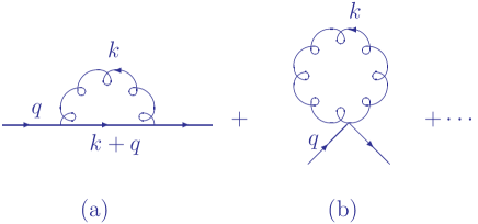
we have shown in Refs. [9, 10, 11] that the large virtual IR effects in the respective loop integrals for the scalar propagator in quantum general relativity can be resummed to the exact result $i\Delta^{\prime}_{F}(k)=\frac{i}{k^{2}-m^{2}-\Sigma_{s}(k)+i\epsilon}=\frac{ie^{B^{\prime\prime}_{g}(k)}}{k^{2}-m^{2}-\Sigma^{\prime}_{s}+i\epsilon}\equiv i\Delta^{\prime}_{F}(k)|_{\text{resummed}}$ for   (here $\Delta=k^{2}-m^{2}$)

$$\begin{split}B^{\prime\prime}_{g}(k)&=-2i\kappa^{2}k^{4}\frac{\int d^{4}\ell}{16\pi^{4}}\frac{1}{\ell^{2}-\lambda^{2}+i\epsilon}\\ &\qquad\frac{1}{(\ell^{2}+2\ell k+\Delta+i\epsilon)^{2}}\\ &=\frac{\kappa^{2}|k^{2}|}{8\pi^{2}}\ln\left(\frac{m^{2}}{m^{2}+|k^{2}|}\right),\end{split}$$ (9)

where the latter form holds for the UV(deep Euclidean) regime, so that $\Delta^{\prime}_{F}(k)|_{\text{resummed}}$ falls faster than any power of $|k^{2}|$ – by Wick rotation, the identification $-|k^{2}|\equiv k^{2}$ in the deep Euclidean regime gives immediate analytic continuation to the result in the last line of (9) when the usual $-i\epsilon,\;\epsilon\downarrow 0,$ is appended to $m^{2}$. An analogous result [9] holds for m=0. Here, $-i\Sigma_{s}(k)$ is the 1PI scalar self-energy function so that $i\Delta^{\prime}_{F}(k)$ is the exact scalar propagator. As $\Sigma^{\prime}_{s}$ starts in ${\cal O}(\kappa^{2})$, we may drop it in calculating one-loop effects. When the respective analogs of $i\Delta^{\prime}_{F}(k)|_{\text{resummed}}$ are used for the elementary particles, one-loop corrections are finite. In fact, the use of our resummed propagators renders all quantum gravity loops UV finite [9, 10, 11]. It is this attendant representation of the quantum theory of general relativity that we have called resummed quantum gravity (RQG).

Indeed, when we use our resummed propagator results, as extended to all the particles in the SM Lagrangian and to the graviton itself, working now with the complete theory ${\cal L}(x)=\frac{1}{2\kappa^{2}}\sqrt{-g}\left(R-2\Lambda\right)+\sqrt{-g}L^{\cal G}_{SM}(x)$ where $L^{\cal G}_{SM}(x)$ is SM Lagrangian written in diffeomorphism invariant form as explained in Refs. [9, 11], we show in the Refs. [9, 10, 11] that the denominator for the propagation of transverse-traceless modes of the graviton becomes ($M_{Pl}$ is the Planck mass) $q^{2}+\Sigma^{T}(q^{2})+i\epsilon\cong q^{2}-q^{4}\frac{c_{2,eff}}{360\pi M_{Pl}^{2}},$ where we have defined $c_{2,eff}=\sum_{\text{SM particles j}}n_{j}I_{2}(\lambda_{c}(j))\cong 2.56\times 10^{4}$ with $I_{2}$ defined [9, 10, 11] by $I_{2}(\lambda_{c})=\int^{\infty}_{0}dxx^{3}(1+x)^{-4-\lambda_{c}x}$ and with $\lambda_{c}(j)=\frac{2m_{j}^{2}}{\pi M_{Pl}^{2}}$ and [9, 10, 11] $n_{j}$ equal to the number of effective degrees of particle $j$. The details of the derivation of the numerical value of $c_{2,eff}$ are given in Refs. [9]. These results allow us to identify (we use $G_{N}$ for $G_{N}(0)$) $G_{N}(k)=G_{N}/(1+\frac{c_{2,eff}k^{2}}{360\pi M_{Pl}^{2}})$ and to compute the UV limit $g_{*}$ as $g_{*}=\lim_{k^{2}\rightarrow\infty}k^{2}G_{N}(k^{2})=\frac{360\pi}{c_{2,eff}}\cong 0.0442.$

For the prediction for $\lambda_{*}$, we use the Euler-Lagrange equations to get Einstein’s equation as

$$G_{\mu\nu}+\Lambda g_{\mu\nu}=-\kappa^{2}T_{\mu\nu}$$ (10)

in a standard notation where $G_{\mu\nu}=R_{\mu\nu}-\frac{1}{2}Rg_{\mu\nu}$, $R_{\mu\nu}$ is the contracted Riemann tensor, and $T_{\mu\nu}$ is the energy-momentum tensor. Working then with the representation $g_{\mu\nu}=\eta_{\mu\nu}+2\kappa h_{\mu\nu}$ for the flat Minkowski metric $\eta_{\mu\nu}=\text{diag}(1,-1,-1,-1)$ we see that to isolate $\Lambda$ in Einstein’s equation (10) we may evaluate its VEV(vacuum expectation value of both sides). On doing this as described in Ref. [22], we see that a scalar makes the contribution to $\Lambda$ given by

$$\begin{split}\Lambda_{s}&=-8\pi G_{N}\frac{\int d^{4}k}{2(2\pi)^{4}}\frac{(2k_{0}^{2})e^{-\lambda_{c}(k^{2}/(2m^{2}))\ln(k^{2}/m^{2}+1)}}{k^{2}+m^{2}}\cr&\cong-8\pi G_{N}[\frac{1}{G_{N}^{2}64\rho^{2}}],\end{split}$$ (11)

where $\rho=\ln\frac{2}{\lambda_{c}}$ and we have used the calculus of Refs. [9, 10, 11]. The standard methods [22] then show that a Dirac fermion contributes $-4$ times $\Lambda_{s}$ to $\Lambda$, so that the deep UV limit of $\Lambda$ then becomes, allowing $G_{N}(k)$ to run, $\Lambda(k)\operatornamewithlimits{\longrightarrow}_{k^{2}\rightarrow\infty}k^{2}\lambda_{*},\;\lambda_{*}=-\frac{c_{2,eff}}{2880}\sum_{j}(-1)^{F_{j}}n_{j}/\rho_{j}^{2}\cong 0.0817$ where $F_{j}$ is the fermion number of $j$, $n_{j}$ is the effective number of degrees of freedom of $j$ and $\rho_{j}=\rho(\lambda_{c}(m_{j}))$. We note that $\lambda_{*}$ would vanish in an exactly supersymmetric theory.

For reference, the UV fixed-point calculated here, $(g_{*},\lambda_{*})\cong(0.0442,0.0817)$, can be compared with the estimates $(g_{*},\lambda_{*})\approx(0.27,0.36)$ in Refs. [17, 18]. In making this comparison, one must keep in mind that the analysis in Refs. [17, 18] did not include the specific SM matter action and that there is definitely cut-off function sensitivity to the results in the latter analyses. What is important is that the qualitative results that $g_{*}$ and $\lambda_{*}$ are both positive and are less than 1 in size are true of our results as well. See Refs. [9] for further discussion of the relationship between our $\{g_{*},\;\lambda_{*}\}$ predictions and those in Refs. [17, 18].

4 Estimate of $\Lambda$ and Constraints on SUSY GUTS

The results here, taken together with those in Refs. [17, 18], allow us to estimate the value of $\Lambda$ today. We take the normal-ordered form of Einstein’s equation

$$:G_{\mu\nu}:+\Lambda:g_{\mu\nu}:=-\kappa^{2}:T_{\mu\nu}:.$$ (12)

The coherent state representation of the thermal density matrix then gives the Einstein equation in the form of thermally averaged quantities with $\Lambda$ given by our result in (11) summed over the degrees of freedom as specified above in lowest order. In Ref. [18], it is argued that the Planck scale cosmology description of inflation gives the transition time between the Planck regime and the classical Friedmann-Robertson-Walker(FRW) regime as $t_{tr}\sim 25t_{Pl}$. (We discuss in Ref. [22]on the uncertainty of this choice of $t_{tr}$.) We thus start with the quantity $\rho_{\Lambda}(t_{tr})\equiv\frac{\Lambda(t_{tr})}{8\pi G_{N}(t_{tr})}=\frac{-M_{Pl}^{4}(k_{tr})}{64}\sum_{j}\frac{(-1)^{F}n_{j}}{\rho_{j}^{2}}$ and employ the arguments in Refs. [32] ($t_{eq}$ is the time of matter-radiation equality) to get the first principles field theoretic estimate

$$\begin{split}\rho_{\Lambda}(t_{0})&\cong\frac{-M_{Pl}^{4}(1+c_{2,eff}k_{tr}^{2}/(360\pi M_{Pl}^{2}))^{2}}{64}\sum_{j}\frac{(-1)^{F}n_{j}}{\rho_{j}^{2}}\cr&\qquad\quad\times\frac{t_{tr}^{2}}{t_{eq}^{2}}\times(\frac{t_{eq}^{2/3}}{t_{0}^{2/3}})^{3}\cr&\cong\frac{-M_{Pl}^{2}(1.0362)^{2}(-9.194\times 10^{-3})}{64}\frac{(25)^{2}}{t_{0}^{2}}\cr&\cong(2.4\times 10^{-3}eV)^{4}.\end{split}$$ (13)

where we take the age of the universe to be $t_{0}\cong 13.7\times 10^{9}$ yrs. In the latter estimate, the first factor in the second line comes from the period from $t_{tr}$ to $t_{eq}$ which is radiation dominated and the second factor comes from the period from $t_{eq}$ to $t_{0}$ which is matter dominated . This estimate should be compared with the experimental result [24] $\rho_{\Lambda}(t_{0})|_{\text{expt}}\cong((2.37\pm 0.05)\times 10^{-3}eV)^{4}$.

To sum up, we believe our estimate of $\rho_{\Lambda}(t_{0})$ represents some amount of progress in the long effort to understand its observed value in quantum field theory. Evidently, the estimate is not a precision prediction, as hitherto unseen degrees of freedom, such as a high scale GUT theory, may exist that have not been included in the calculation.

Indeed, what would happen to our estimate if there were a GUT theory at high scale? As is well-known, the main viable approaches involve susy GUT’s and for definiteness, we will use the susy SO(10) GUT model in Ref. [34] to illustrate how such theory might affect our estimate of $\Lambda$. In this model, the break-down of the GUT gauge symmetry to the low energy gauge symmetry occurs with an intermediate stage with gauge group $SU_{2L}\times SU_{2R}\times U_{1}\times SU(3)^{c}$ where the final break-down to the Standard Model [35, 36] gauge group, $SU_{2L}\times U_{1}\times SU(3)^{c}$, occurs at a scale $M_{R}\gtrsim 2TeV$ while the breakdown of global susy occurs at the (EW) scale $M_{S}$ which satisfies $M_{R}>M_{S}$. The key observation is that only the broken susy multiplets can contribute to $\rho_{\Lambda}(t_{tr})$ . In the model at hand, these are just the multiplets associated with the known SM particles and the extra Higgs multiplet required by susy in the MSSM [37]. In view of recent LHC results [38], we take for illustration the values $M_{R}\cong 4M_{S}\sim 2.0{\text{TeV}}$ and set the following susy partner values: $m_{\tilde{g}}\cong 1.5(10){\text{TeV}},\;m_{\tilde{G}}\cong 1.5{\text{TeV}},\;m_{\tilde{q}}\cong 1.0{\text{TeV}},\;m_{\tilde{\ell}}\cong 0.5{\text{TeV}},\;m_{\tilde{\chi}^{0}_{i}}\cong\begin{cases}&0.4{\text{TeV}},\;i=1\\ &0.5{\text{TeV}},\;i=2,3,4\end{cases},\;m_{\tilde{\chi}^{\pm}_{i}}\cong 0.5{\text{TeV}},\;i=1,2,\;m_{S}=.5{\text{TeV}},\;S=A^{0},\;H^{\pm},\;H_{2},$ where we use a standard notation for the susy partners of the known quarks($q\leftrightarrow\tilde{q}$), leptons($\ell\leftrightarrow\tilde{\ell}$) and gluons($G\leftrightarrow\tilde{G}$), and the EW gauge and Higgs bosons($\gamma,\;Z^{0},\;W^{\pm},\;H,$ $A^{0},\;H^{\pm},\;H_{2}\leftrightarrow\tilde{\chi}$) with the extra Higgs particles denoted as usual [37] by $A^{0}$(pseudo-scalar), $H^{\pm}$(charged) and $H_{2}$(heavy scalar). $\tilde{g}$ is the gravitino, for which we show two examples of its mass for illustration. These particles then generate the extra contribution $\Delta W_{\rho,\text{GUT}}=\sum_{j\in\{\text{MSSM low energy susy partners}\}}\frac{(-1)^{F}n_{j}}{\rho_{j}^{2}}\cong 1.13(1.12)\times 10^{-2}$ to the factor $W_{\rho}\equiv\sum_{j}\frac{(-1)^{F}n_{j}}{\rho_{j}^{2}}$ on the RHS of our equation for $\rho_{\Lambda}(t_{tr})$ for the two respective values of $m_{\tilde{g}}$ called out by the parentheses. The corresponding values of $\rho_{\Lambda}$ are $-(1.67\times 10^{-3}\text{eV})^{4}(-(1.65\times 10^{-3}\text{eV})^{4})$, respectively. The sign of these results would appear to put them in conflict with the positive observed value quoted above by many standard deviations, even when we allow for the considerable uncertainty in the various other factors multiplying $W_{\rho}$ in our formula for $\rho_{\Lambda}(t_{tr})$, all of which are positive. This may be alleviated either by adding new particles to the model, approach (A), or by allowing a soft susy breaking mass term for the gravitino that resides near the GUT scale $M_{GUT}$, which is $\sim 4\times 10^{16}GeV$ here [34], approach (B). In approach (A), we double the number of quarks and leptons, but we invert the mass hierarchy between susy partners, so that the new squarks and sleptons are lighter than the new quarks and leptons. This can work as long as as we increase $M_{R},\;M_{S}$ so that we have the new quarks and leptons at $M_{\text{High}}\sim 3.4(3.3)\times 10^{3}\text{TeV}$ while leaving their partners at $M_{\text{Low}}\sim.5{\text{TeV}}$. For approach (B), the mass of the gravitino soft breaking term should be set to $m_{\tilde{g}}\sim 2.3\times 10^{15}{\text{GeV}}$. More generally, our estimate in (13) can be used as a constraint of general susy GUT models and we hope to explore such in more detail elsewhere.

As we explain in Ref. [22], our uncertainty on the value of $t_{tr}$ at the level of a couple of orders of magnitude translates to an uncertainty at the level of $10^{4}$ on our estimate of $\rho_{\Lambda}$.

The effect of the various spontaneous symmetry vacuum energies on our $\rho_{\Lambda}$ estimate can be addressed as follows. The energy of the broken vacuum for the EW (GUT) case contributes an amount of order $M_{W}^{4}$ ($M_{GUT}^{4}$) to $\rho_{\Lambda}$. When compared to the RHS of our equation for $\rho_{\Lambda}(t_{tr})$, which is $\sim(-(1.0362)^{2}W_{\rho}/64)M_{Pl}^{4}\simeq\frac{10^{-2}}{64}M_{Pl}^{4}$, we see that adding these effects thereto would make relative changes in our results at the level of $\frac{64}{10^{-2}}\frac{M_{W}^{4}}{M_{Pl}^{4}}\cong 1\times 10^{-65}$ and $\frac{64}{10^{-2}}\frac{M_{GUT}^{4}}{M_{Pl}^{4}}\cong 7\times 10^{-7}$, respectively, where we use the value of $M_{GUT}$ above for definiteness. Such small effects are ignored here.

Concerning the impact of our approach to $\Lambda$ on the phenomenology of big bang nucleosynthesis(BBN) [39], we recall that the authors in Ref. [18] have already noted that, when one passes from the Planck era to the FRW era, a gauge transformation (from the attendant diffeomorphism invariance) is necessary to maintain consistency with the solutions of the system (LABEL:coseqn1)(or of its more general form discussed below) at the boundary $t_{tr}$ between the two regimes. Requiring that the Hubble parameter be continuous at $t_{tr}$ the authors in Ref. [18] arrive at the gauge transformation on the time for the FRW era relative to the Planck era $t\rightarrow t^{\prime}=t-t_{as}$ so that continuity of the Hubble parameter at the boundary gives $\frac{\alpha}{t_{tr}}=\frac{1}{2(t_{tr}-t_{as})}$ when $a(t)\propto t^{\alpha}$ in the (sub-)Planck regime. This implies $t_{as}=(1-\frac{1}{2\alpha})t_{tr}.$ In our case , we have from Ref. [18] the generic case $\alpha=25$, so that $t_{as}=0.98t_{tr}.$ Here, we use the diffeomorphism invariance of the theory to choose another coordinate transformation for the FRW era, namely, $t\rightarrow t^{\prime}=\gamma t$ as a part of a dilatation where $\gamma$ now satisfies the boundary condition required for continuity of the Hubble parameter at $t_{tr}$: $\frac{\alpha}{t_{tr}}=\frac{1}{2\gamma t_{tr}}$ so that $\gamma=\frac{1}{2\alpha}.$ The model in Ref. [18] purports that, for $t>t_{tr}$, one has the time $t^{\prime}$ and an effective FRW cosmology with such a small value of $\Lambda$ that it may be treated as zero. Here, we extend this by retaining $\Lambda\neq 0$ so that we may estimate its value. But, with our diffeomorphism transformation between the (sub-)Planck regime and the FRW regime, we can see that, at the time of BBN, the ratio of $\rho_{\Lambda}$ to $\frac{3H^{2}}{8\pi G_{N}}$ is

$$\begin{split}\Omega_{\Lambda}(t_{BBN})&=\frac{M_{Pl}^{2}(1.0362)^{2}9.194\times 10^{-3}(25)^{2}/(64t_{BBN}^{2})}{(3/(8\pi G_{N}))(1/(2\gamma t_{BBN})^{2})}\cr&\cong\frac{\pi 10^{-2}}{24}\cr&=1.31\times 10^{-3}.\end{split}$$ (14)

Thus, at $t_{BBN}$ our $\rho_{\Lambda}$ is small enough that it has a negligible effect on the standard BBN phenomenology.

Turning next to the issue of the covariance of the theory when $\Lambda$ and $G_{N}$ depend on time, we follow in Eqs.(LABEL:coseqn1) the corresponding realization of the improved Friedmann and Einstein equations as given in Eqs.(3.24) in Ref. [17]. The more general realization of (LABEL:coseqn1) is given in Eqs.(2.1) in Ref. [18] – our discussions in this Section effectively followed the latter realization. The two realizations differ in the solution of the Bianchi identity constraint: $D^{\nu}\left(\Lambda g_{\nu\mu}+8\pi G_{N}T_{\nu\mu}\right)=0;$ for, this identity is solved in (LABEL:coseqn1) for a covariantly conserved $T_{\mu\nu}$ as well whereas, in Eqs.(2.1) in Ref. [18], one has the modified conservation requirement $\dot{\rho}+3\frac{\dot{a}}{a}(1+\omega)\rho=-\frac{\dot{\Lambda}+8\pi\rho\dot{G}_{N}}{8\pi G_{N}};$ in (LABEL:coseqn1) the RHS of this latter equation is set to zero. The phenomenology from Ref. [17] is qualitatively unchanged by the simplification in (LABEL:coseqn1) but the attendant details, such as the (sub-)Planck era exponent for the time dependence of $a$, etc., are affected, as is the relation between $\dot{\Lambda}$ and $\dot{G}_{N}$ in (LABEL:coseqn1). We note that (LABEL:coseqn1) contains a special case of the more general realization of the Bianchi identity requirement when both $\Lambda$ and $G_{N}$ depend on time and in this Section we use that more general realization. We also note that only when $\dot{\Lambda}+8\pi\rho\dot{G}_{N}=0$ holds is covariant conservation of matter in the current universe guaranteed and that either the case with or the case without such guaranteed conservation is possible provided the attendant deviation is small. See Refs. [40, 41, 42] for detailed studies of such deviation, including its maximum possible size.

We stress that the model Planck scale cosmology of Bonanno and Reuter which we use needs more work to remove the type of uncertainties which we just elaborated in our estimate of $\Lambda$. We thank Profs. L. Alvarez-Gaume and W. Hollik for the support and kind hospitality of the CERN TH Division and the Werner-Heisenberg-Institut, MPI, Munich, respectively, where a part of this work was done.

References

- [1] S. Weinberg, in General Relativity, an Einstein Centenary Survey, eds. S. W. Hawking and W. Israel, (Cambridge Univ. Press, Cambridge, 1979).
- [2] M. Reuter, Phys. Rev. D57 (1998) 971, and references therein.
- [3] O. Lauscher and M. Reuter, Phys. Rev. D66 (2002) 025026.
- [4] E. Manrique, M. Reuter and F. Saueressig, Ann. Phys. 326 (2011) 44, and references therein.
- [5] A. Bonanno and M. Reuter, Phys. Rev. D62 (2000) 043008.
- [6] D. F. Litim, Phys. Rev. Lett.92(2004) 201301; Phys. Rev. D64 (2001) 105007; P. Fischer and D.F. Litim, Phys. Lett. B638 (2006) 497 and references therein.
- [7] D. Don and R. Percacci, Class. Quant. Grav. 15 (1998) 3449; R. Percacci and D. Perini, Phys. Rev. D67(2003) 081503; ibid.68 (2003) 044018; R. Percacci, ibid.73(2006) 041501; A. Codello, R. Percacci and C. Rahmede, Int.J. Mod. Phys. A23(2008) 143.
- [8] K. G. Wilson, Phys. Rev. B4 (1971) 3174, 3184; K. G. Wilson, J.Kogut, Phys. Rep. 12 (1974) 75; F. Wegner, A. Houghton, Phys. Rev. A8(1973) 401; S. Weinberg, “Critical Phenomena for Field Theorists”, Erice Subnucl. Phys. (1976) 1; J. Polchinski, Nucl. Phys. B231 (1984) 269.
- [9] B.F.L. Ward, Open Nucl.Part.Phys.Jour. 2(2009) 1.
- [10] B.F.L. Ward, Mod. Phys. Lett. A17 (2002) 237.
- [11] B.F.L. Ward, Mod. Phys. Lett. A19 (2004) 143.
- [12] B.F.L. Ward, Mod. Phys. Lett. A23 (2008) 3299.
- [13] D. R. Yennie, S. C. Frautschi, and H. Suura, Ann. Phys. 13 (1961) 379; see also K. T. Mahanthappa, Phys. Rev. 126 (1962) 329, for a related analysis.
- [14] S. Jadach and B.F.L. Ward, Phys. Rev. D38 (1988) 2897;ibid. D39 (1989) 1471; ibid. D40 (1989) 3582; Comp. Phys. Commun. 56 (1990) 351; S.Jadach, B.F.L. Ward and Z. Was, Comput. Phys. Commun. 66 (1991) 276; ibid. 79 (1994) 503; ibid. 124 (2000) 233; ibid.130 (2000) 260; Phys. Rev.D63 (2001) 113009; S.Jadach, W. Placzek and B.F.L. Ward, Phys. Lett. B390 (1997) 298; S. Jadach et al., Phys. Lett. B417 (1998) 326; Comput. Phys. Commun. 119 (1999) 272; ibid.140 (2001) 432, 475; Phys. Rev. D61 (2000) 113010; ibid. D65 (2002) 093010.
- [15] J. Ambjorn et al., Phys. Lett. B690 (2010) 420.
- [16] P. Horava, Phys. Rev. D 79 (2009) 084008.
- [17] A. Bonanno and M. Reuter, Phys. Rev. D65 (2002) 043508.
- [18] A. Bonanno and M. Reuter, Jour. Phys. Conf. Ser. 140 (2008) 012008, and references therein.
- [19] I. L. Shapiro and J. Sola, Phys. Lett. B475 (2000) 236.
- [20] See for example A. H. Guth and D.I. Kaiser, Science 307 (2005) 884; A. H. Guth, Phys. Rev. D23 (1981) 347.
- [21] See for example A. Linde, Lect. Notes. Phys. 738 (2008) 1.
- [22] B.F.L. Ward, Phys. Dark Univ. 2 (2013) 97.
- [23] A.G. Riess et al., Astron. Jour. 116 (1998) 1009; S. Perlmutter et al., Astrophys. J. 517 (1999) 565.
- [24] C. Amsler et al., Phys. Lett. B667 (2008) 1.
- [25] B.F.L. Ward, to appear.
- [26] S. Weinberg, The Quantum Theory of Fields, v.1,(Cambridge University Press, Cambridge, 1995).
- [27] R.P. Feynman, Acta Phys. Pol.24 (1963) 697-722.
- [28] R.P. Feynman, Lectures on Gravitation, eds. F.B. Moringo and W.G. Wagner WG, (Caltech, Pasadena, 1971).
- [29] L.D. Faddeev and V.N. Popov, “Perturbation theory for gauge invariant fields”, preprint ITF-67-036, NAL-THY-57 (translated from Russian by D. Gordon and B.W. Lee). Available from http://lss.fnal.gov/archive/test-preprint/fermilab-pub-72-057-t.shtml.
- [30] Faddeev LD and Popov VN. Feynman diagrams for the Yang-Mills field. Phys Lett B 1967; 25: 29-30.
- [31] Ya. B. Zeldovich, Sov. Phys. Uspekhi 11 (1968) 381.
- [32] V. Branchina and D. Zappala, G. R. Gravit. 42 (2010) 141; arXiv:1005.3657, and references therein.
- [33] J. Sola, J. Phys. A41 (2008) 164066.
- [34] P.S. Bhupal Dev and R.N. Mohapatra, Phys. Rev. D82 (2010) 035014, and references therein.
- [35] S.L. Glashow, Nucl. Phys. 22 (1961) 579; S. Weinberg, Phys. Rev. Lett. 19 (1967) 1264; A. Salam, in Elementary Particle Theory, ed. N. Svartholm (Almqvist and Wiksells, Stockholm, 1968), p. 367; G. ’t Hooft and M. Veltman, Nucl. Phys. B44,189 (1972) and 50, 318 (1972); G. ’t Hooft, ibid. 35, 167 (1971); M. Veltman, ibid. 7, 637 (1968).
- [36] D. J. Gross and F. Wilczek, Phys. Rev. Lett. 30 (1973) 1343; H. David Politzer, ibid.30 (1973) 1346; see also , for example, F. Wilczek, in Proc. 16th International Symposium on Lepton and Photon Interactions, Ithaca, 1993, eds. P. Drell and D.L. Rubin (AIP, NY, 1994) p. 593.
- [37] See for example H.E. Haber and G.L. Kane, Phys. Rep.117 (1985) 75, and references therein.
- [38] See for example S. Lowette, in Proc. Rencontres de Moriond EW 2012, in press.
- [39] See for example G. Stiegman, Ann. Rev. Nucl. Part. Sci.57 (2007) 463, and references therein.
- [40] S. Basilakos, M. Plionis and J. Sola, arXiv:0907.4555.
- [41] J. Grande et al., J. Cos. Astropart. Phys. 1108 (2011) 007.
- [42] H. Fritzsch and J. Sola, arXiv:1202.5097, and references therein.