A Sample of Type II-L Supernovae

Abstract

What are Type II-Linear supernovae (SNe II-L)? This class, which has been ill defined for decades, now receives significant attention — both theoretically, in order to understand what happens to stars in the $\sim 15$–25 M_⊙ range, and observationally, with two independent studies suggesting that they cannot be cleanly separated photometrically from the regular hydrogen-rich SNe II-P characterised by a marked plateau in their light curve. Here, we analyze the multi-band light curves and extensive spectroscopic coverage of a sample of 35 SNe II and find that 11 of them could be SNe II-L. The spectra of these SNe are hydrogen deficient, typically have shallow H$\alpha$ absorption, may show indirect signs of helium via strong O I $\lambda$7774 absorption, and have faster line velocities consistent with a thin hydrogen shell. The light curves can be mostly differentiated from those of the regular, hydrogen-rich SNe II-P by their steeper decline rates and higher luminosity, and we propose as a defining photometric characteristic the decline in the $V$ band: SNe II-L seem to decline by more than 0.5 mag from peak brightness by day 50 after explosion. Using our sample we provide template light curves for SNe II-L and II-P in 4 photometric bands.

1 Introduction

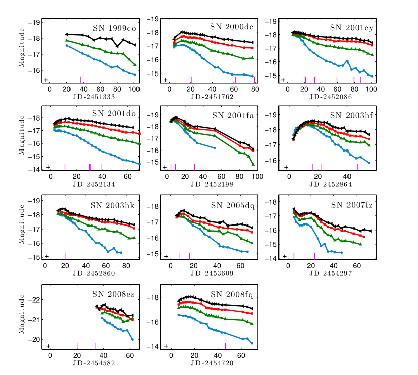
Figure 1: Light curves for the 11 SNe in our sample: $B$ (blue circles), $V$ (green triangles), $R$ (red squares), and $I$ (black side triangles). Magenta ticks mark the epochs at which spectra were obtained. The cross signs mark the last nondetection day.

Core-collapse supernovae (SNe) are divided into an array of subtypes based on their observational properties. This could be seen as a trivial and pedantic exercise; however, when ultimately trying to decipher the fate of massive stars, as well as their interplay with their surroundings, one needs to be able to draw a clear mapping from progenitor to SN. The accepted classification scheme is mostly spectroscopic, based on the presence of hydrogen (Type II) or lack of it (Types Ib and Ic). Some Type II SNe are further assigned a subtype based on the presence of relatively narrow emission lines (IIn) or having intermediate properties — starting off as a Type II, evolving into a Ib (IIb). To further complicate the picture, there is a photometric distinction between SNe II-P that have a long period of roughly constant luminosity (a plateau) and SNe II-L with a linearly (in magnitudes) declining light curve (see Filippenko 1997 for a review).

Clearly, spectroscopic classes and photometric classes are not necessarily mutually exclusive. An object could in principle have a linearly declining light curve, supposedly making it a SN II-L, and yet spectroscopically resemble other classes (IIb or IIn). The spectroscopic signature of SNe II-L (if indeed they form an independent class) is ill defined. [An exception to this is tentative evidence that SN II-L spectra do not show a well-developed H$\alpha$ absorption component in the P-Cygni line profile (Schlegel 1996).] Thus, mostly owing to the time required to acquire, calibrate, and analyze a light curve (as opposed to the nearly instantaneous spectroscopic analysis), the SN II-L class has been largely unassigned for decades.

A major impediment to detailed studies of SNe II-L is that they are rare, though not as rare as might appear from a casual literature search. Out of 1154 unambiguous Type II classifications reported to the IAU between the years 2000 and 2013, 697 are not assigned a subtype, 228 are II-P, 158 are IIn, 68 are IIb, and only 3 are II-L. This is a direct consequence of the lack of a spectroscopic definition of SNe II-L, and it suggests a rate among SNe II of less than a percent. However, having redefined SNe II-L as objects that decline by $\sim 1$ mag over 100 days (Poznanski et al. 2009), Li et al. (2011) find that while SNe II-P comprise about 60% of all core-collapse events, SNe II-L still constitute a few percent (see also Smartt 2009).

The prevalence of SNe II-P is compatible with our current understanding that their progenitors are also the most common massive stars (the least massive ones): red supergiants (RSGs) with masses of 8–15 M_⊙, a link strongly established by progenitor detections (Smartt 2009). In contrast, there is only weak evidence regarding the progenitors of SNe II-L. SN 1979C (e.g., Branch et al. 1981) and SN 1980K (e.g., Uomoto & Kirshner 1986) are the nearest and best-observed “historical” SNe II-L. The position of SN 1980K was imaged 49 days before maximum light (Thompson 1982), but no star was found to be coincident with the position of the SN, ruling out RSGs more massive than 20 M_⊙ though allowing bluer progenitors with $T>$ 10,000 K and a mass in the range of 10–15 M_⊙ (Smartt 2009). An analysis of the stellar population around SN 1979C shows that with the exception of one supergiant, most of the stars appear to be massive main-sequence turnoff stars. Hence, the progenitor of SN 1979C was likely a RSG with mass $\sim 17$–18 M_⊙ (Van Dyk et al. 1999).

The only “modern” (i.e., post Hubble Space Telescope) SN II-L with a progenitor detected is SN 2009kr (Elias-Rosa et al. 2010; Fraser et al. 2010). There is debate regarding the interpretation of the observations. While Elias-Rosa et al. (2010) favor a massive progenitor of 18–24 M_⊙, Fraser et al. (2010) argue that if the progenitor is a single star, then it is a yellow supergiant with a mass of $15^{+5}_{-4}\,{\rm M}_{\odot}$. Based on the mass-velocity relation (which suggests that the progenitor mass is proportional to the day 50 photospheric velocity, $M\propto v$), Poznanski (2013) argue that the higher mass is favored.

The distribution of SN II-P progenitor masses (see the compilation by Smartt 2009 and Table 1 of Poznanski 2013) spans masses approximately between 8 M_⊙ and 18 M_⊙ with an upper limit of 25 M_⊙. The few SN II-L progenitor masses are thus at the higher end of this distribution, perhaps just beyond it.

There is a paucity of progenitor detections with masses greater than $\sim 15$ M_⊙, as well as an observed gap in the the masses of stellar remnants. Neutron star (NS) masses reach about 2M_⊙, while black hole (BH) masses seem to start near 5 M_⊙ (Özel et al. 2010, 2012). A compelling solution to these two mysteries was suggested (see Kochanek 2013, and references therein). If above some mass threshold stars fail to produce a SN, and collapse directly to form a BH, they accumulate more mass in the core, thus explaining the perceived lack of progenitors as well as the gap in remnant masses. Based on the rate determinations of Li et al. (2011), Smith et al. (2011) argue that there is no gap when translating the SN rates to the initial mass function; however, Kochanek (2013) dismisses this argument, claiming that the uncertainty in the fraction of SNe coming from binaries could allow for the needed adjustment. This discussion is significantly hampered by the uncertain definition and poorly studied properties of SNe II-L. Understanding SNe II-L, their progenitors, and where they fit in the progenitor-to-SN mapping is our main purpose here..

As one goes up the mass function, wind-induced mass loss becomes a dominant process, particularly during the RSG phase. In fact, models show that stars more massive than $\sim 20$ M_⊙ can end up with less mass than their less-massive siblings, after having lost most or all of their hydrogen outer shells. The remaining thin hydrogen envelopes are further helium enriched by convective dredge-up from the helium shell to the outer envelope (e.g., Kasen & Woosley 2009). This has a direct effect on the helium mass fraction, since the helium-core mass is an increasing function of the initial mass.

The photometric plateau of SNe II-P is interpreted as being powered by a hydrogen recombination wave propagating inward through the SN envelope, slowly releasing all the energy deposited by the shock (e.g., Popov 1993; Kasen & Woosley 2009). A thinner hydrogen envelope, as one would expect from a more massive progenitor, cannot support a long plateau phase, releasing the trapped energy faster. Furthermore, the abundance of helium in the envelope alters the electron-scattering opacity and the recombination temperature of the ejecta, since the recombination temperature of helium is higher than that of hydrogen ($\sim$ 10,000–12,000 K; Arnett 1996).

In a recent numerical study, Bayless et al. (2014) tested the effects of mass loss on the light curve of a SN with a progenitor of 23 M_⊙ (initial mass). They found that removing hydrogen from the outer shell gradually alters the nature of the light curve from II-P to IIb/Ib, where the decline rate of the light curve correlates with mass loss.

Therefore, SNe from progenitors near $\sim 20$ M_⊙ should be more luminous than SNe II-P, have more rapidly declining light curves, and display evidence of helium, all due to the thin hydrogen shell. As already suggested by Patat et al. (1994) and as we show below, SNe II-L consistently fit this picture.

Recently, as this paper was in its final editing stages, two groups published large samples of SNe II (Anderson et al. 2014; Sanders et al. 2014). Both found that contrary to previous claims (the latest by Arcavi et al. 2012), one cannot photometrically separate SNe II-L from SNe II-P. While our sample is smaller and we cannot make definitive conclusions, we address this issue as well. Gutiérrez et al. (2014) focus on a spectroscopic study of the H$\alpha$ line, using a somewhat larger sample than ours, and find results which are consistent with those we present below.

2 Observations

The sample of SNe was compiled from data collected with the 0.76-m Katzman Automatic Imaging Telescope (KAIT), as a part of the Lick Observatory SN search. A sample of 35 SNe II was constructed, excluding SNe IIb and IIn based on spectroscopic identifications. In a companion paper (Faran 2014, hereafter F14a) we analyze in detail the 23 SNe II-P in the sample and discuss all of the observational and reduction details. SN 2000cb, a SN 1987A analog, is analyzed by Kleiser et al. (2011). The remaining 11 SNe are discussed here, and listed in Table 1. As explained in detail by F14a, the photometry is corrected for Galactic extinction using the maps of Schlegel, Finkbeiner & Davis (1998), but we do not correct for host-galaxy extinction. All photometric and spectroscopic data are available electronically via the Berkeley (Silverman et al. 2012) and WISeREP (Yaron & Gal-Yam 2012) databases. Table 2 includes a sample of the photometric data. The full table is available in the online version. The journal of spectroscopic observations is included in Table 3.

Table 1: SN II-L Sample

SN name	$z_{\rm host}$	$\mu$ (mag)	Explosion MJD	$E(B-V)_{\rm MW}$
1999co	0.0314	35.52b	51332 (5)	0.0490
2000dc	0.0104	33.52	51762 (4)	0.0796
2001cy	0.0149	33.94b	52085 (6)	0.1983
2001do	0.0104	33.16b	52133 (2)	0.1950
2001fa	0.0173	34.58	52198 (3)	0.0770
2003hf	0.0313	35.55b	52863 (2)	0.0220
2003hk	0.0226	35.07	52860 (?)	0.0335
2005dq	0.0219	34.77b	53608 (4)	0.0803
2007fz	0.0144	33.86b	54296 (3)	0.0402
2008es	0.2130	39.38b	54581 (1)	0.0117
2008fq	0.0106	32.86	54720 (5)	0.0637

Table 2: Sample light curves.

SN name	MJD	Age	B($\sigma_{B}$)	V($\sigma_{V}$)	R($\sigma_{R}$)	I($\sigma_{I}$)
2001cy	52091.44	6.4	15.918(0.026)	15.958(0.021)	15.828(0.017)	15.779(0.037)
2001cy	52092.48	7.5	15.988(0.030)	15.809(0.018)	15.817(0.014)	15.738(0.029)
2001cy	52093.44	8.4	15.967(0.042)	15.976(0.036)	15.841(0.044)	15.770(0.034)
…	…	…	…	…	…
2001do	52136.25	3.1	16.127(0.030)	15.924(0.022)	15.719(0.016)	15.618(0.020)
2001do	52137.27	4.1	16.187(0.039)	15.898(0.017)	15.665(0.013)	15.521(0.020)
2001do	52138.24	5.0	16.174(0.031)	15.828(0.017)	15.615(0.016)	15.432(0.016)
…	…	…	…	…	…
2001fa	52202.35	4.5	16.070(0.014)	16.185(0.014)	16.157(0.018)	16.190(0.020)
2001fa	52203.34	5.4	16.012(0.012)	16.122(0.011)	16.070(0.012)	16.039(0.014)
2001fa	52204.36	6.5	16.051(0.013)	16.067(0.010)	15.996(0.016)	15.955(0.011)
…	…	…	…	…	…
2005dq	53613.31	5.2	17.355(0.019)	17.483(0.042)	17.474(0.028)	17.358(0.056)
2005dq	53614.32	6.2	17.358(0.030)	17.400(0.033)	17.399(0.025)	17.355(0.080)
2005dq	53615.28	7.2	17.417(0.023)	17.421(0.039)	17.365(0.022)	17.214(0.059)
…	…	…	…	…	…

In order to distinguish between SNe II-L and II-P, we photometrically define an object as a SN II-L if its $V$-band light curve declines by more than 0.5 mag from peak brightness during the first 50 days after explosion. The division is not very sensitive to this choice (see Section 3.1).

In Figure 1 we show the $BVRI$ light curves of the 11 objects in our sample, marking at the bottom of each plot the epochs at which spectra were taken. Table 1 includes the redshifts, distances, and explosion dates. Most of the objects are at low redshifts with $z<0.03$, except for the very luminous SN 2008es at $z=0.213$ (Miller et al. 2009; Gezari et al. 2009). The explosion day is set as the midpoint between the first detection and the last non detection. In case a constraining nondetection is not available, as for SN 2003hk, a rough estimate for the explosion day is obtained by comparing the epoch of peak brightness to that of SNe with similar light curves. Distance measurements are collected from NED, where we use the mean value of distances based on the Tully-Fisher method, Cepheid variable stars, and SNe Ia.

Table 3: Journal of Spectroscopic Observations

SN Name	MJD	Age (Days)	Instrument	Range (Å)	Exposure (s)
1999co	51368.45	36.5	Kast	4320-7030	1200
2000dc	51782.25	20.4	Kast	3290-10450	900
2000dc	51823.18	61.4	Kast	3300-7790	1800
2000dc	51841.11	79.3	Kast	3300-7800	2400
2001cy	52106.48	21.5	Kast	3300-10400	900
2001cy	52117.42	32.4	Kast	3300-10400	900
2001cy	52144.45	59.4	Kast	3300-10400	900
2001cy	52164.25	79.2	Kast	3300-10400	900
2001cy	52172.32	87.3	Kast	3300-10400	900
2001cy	52207.12	122.1	Kast	3280-10400	1500
2001do	52144.41	11.2	Kast	3300-10400	600
2001do	52163.23	30.0	Kast	3300-10400	600
2001do	52164.19	31.0	Kast	3300-10400	600
2001do	52172.30	39.1	Kast	3300-10400	1000
2001fa	52202.25	4.3	Kast	3300-10400	900
2001fa	52204.00	6.1	ESI	3930-10198	300
2001fa	52205.00	7.1	ESI	3930-10199	200
2001fa	52228.39	30.5	Kast	3280-10400	600
2001fa	52288.00	90.1	Kast	3268-10570	2700
2003hf	52879.20	16.0	Kast	3252-10600	1200
2003hf	52885.29	22.1	Kast	3232-10400	1500
2003hf	52910.00	46.8	LRIS	3164-9250	300
2003hk	52879.42	19.9	Kast	3254-10218	1200
2005dq	53615.34	7.2	Kast	3310-10500	1800
2005dq	53624.38	16.3	Kast	3350-10400	1500
2005dq	53682.00	73.9	DEIMOS	4900-10061	900
2007fz	54301.20	5.1	Kast	3320-10600	1200
2007fz	54319.24	23.1	Kast	3326-10600	1500
2007fz	54326.00	29.9	Kast	3420-10130	1500
2007fz	54333.00	36.9	Kast	3398-10500	1500
2008es	54602.00	20.6	Kast	3296-10800	1500
2008es	54615.00	33.6	Kast	3298-10800	1800
2008es	54654.25	72.9	Kast	3306-10800	2100
2008es	54624.00	42.6	LRIS	3102-9228	600
2008es	54638.00	56.6	R.C.S	3764-9444	900
2008es	54681.00	99.6	LRIS	3100-9190	405
2008fq	54766.20	46.4	LRIS	3138-9156	120
2008fq	54739.00	19.2	Kast	3408-10770	900
2008fq	54746.00	26.2	Kast	3410-10780	1200
2008fq	54761.00	41.2	Kast	3428-6404	2400
2008fq	54777.00	57.2	Kast	3726-10800	1200
2008fq	54790.00	70.2	Kast	3480-10000	1500

3 Photometric Properties

Figure 2 presents the luminosity function in the $I$ band, comparing the peak magnitudes of the SNe II-L to the mean plateau magnitude of SNe II-P in F14a. Even without the superluminous SN 2008es, the SNe II-L are more luminous than SNe II-P by about 1.5 mag at peak, which has been previously shown in Anderson et al. (2014) and Patat et al. (1994), and more uniform, though the sample is smaller and the subtypes overlap. The data used for this plot are presented in Table LABEL:t:data.

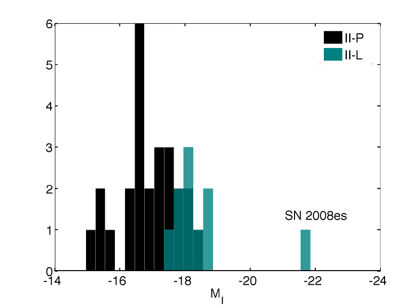
Figure 2: $I$-band absolute magnitude light curves. SNe II-P (black) seem to cover a range of 3 mag (between $-18$ and $-15$ mag) and are $\sim 1.5$ mag dimmer than SNe II-L (green).

In Figure 3 we compare the colour evolution of the SNe II-L to the SNe II-P from F14a. Aside from a small gap of $\sim 0.07$ mag on average (over time), the two subtypes seem to evolve the same way. Since some of the events do not have $R$-band photometry, we only use objects with data in all four bands in order to be consistent when plotting different colours. Therefore, for SNe II-P we are able to average over a maximum of 11 events per day, and 8 for SNe II-L. The plot terminates on day 70, since beyond this day the mean SN II-L colour is determined by only 3 SNe and might be highly affected by individual objects.

The similar evolution of the SN II-P and II-L colours is not trivial to interpret, since the light curves of the two classes have quite different shapes. The redder colour of SNe II-L could be intrinsic or caused by a different typical extinction. The latter possibility is consistent with the high mean equivalent width of Na I D absorption (2.02 Å) we find for 5 SNe II-L, following the methods of F14a. An especially high value of 3.72 Å is obtained for SN 2008fq. The mean for the 13 SNe II-P in F14a, 1.10 Å, is significantly lower. If sodium absorption correlates with dust column density (Turatto, Benetti & Cappellaro 2003; Poznanski et al. 2011; Poznanski, Prochaska & Bloom 2012), this is an indication that SNe II-L reside in dustier areas, closer to their birth sites, as one would expect from more massive stars. Alternatively, the Na I D in SNe II-L could be partly circumstellar, due to more substantial mass loss.

Table 4: Photometric Properties

SN Name	MI,max	Decline ($I$; mag/50 d)	Decline ($V$; mag/50 d)
1999bg	-16.61(0.40)	0.11(0.02)	0.33(0.01)
1999co	-18.24(0.22)	0.38(0.09)	0.77(0.05)
1999d	-	-	-
1999em	-16.75(0.36)	-0.13(0.01)	0.19(0.00)
1999gi	-15.61(0.31)	-0.02(0.01)	0.36(0.02)
2000bs	-17.83(0.22)	-0.02(0.04)	0.30(0.02)
2000dc	-18.02(0.31)	0.62(0.04)	0.94(0.13)
2000dj	-17.26(0.22)	0.06(0.03)	0.38(0.03)
2001bq	-17.35(0.22)	-0.08(0.02)	0.24(0.02)
2001cm	-17.25(0.37)	-0.07(0.02)	0.37(0.03)
2001cy	-18.20(0.22)	0.35(0.01)	0.82(0.01)
2001do	-17.95(0.22)	0.72(0.02)	1.25(0.02)
2001fa	-18.75(0.01)	1.41(0.03)	1.99(0.03)
2001hg	-16.81 0.29	-	-
2001x	-16.64(0.28)	-0.04(0.01)	0.21(0.01)
2002an	-17.83(0.05)	-	-
2002bx	-18.42 0.42	-	-
2002ca	-16.27(0.22)	0.05(0.03)	0.39(0.03)
2002gd	-16.39(0.21)	0.11(0.02)	0.25(0.05)
2002hh	-15.32(0.19)	0.01(0.05)	0.31(0.06)
2003gd	-16.51 0.23	-	-
2003hf	-18.58(0.22)	1.24(0.06)	2.00(0.04)
2003hk	-18.41(0.06)	0.79(0.02)	1.23(0.02)
2003hl	-17.17(0.30)	0.03(0.01)	0.37(0.01)
2003iq	-17.57(0.30)	0.04(0.01)	0.37(0.01)
2003z	-15.20(0.20)	-0.26(0.03)	0.19(0.02)
2004du	-18.07(0.33)	0.09(0.02)	0.48(0.02)
2004et	-17.53(0.19)	-0.05(0.00)	0.36(0.00)
2005ay	-16.52(0.40)	-0.14(0.01)	0.19(0.01)
2005cs	-15.52(0.07)	-	0.26(0.01)
2005dq	-17.72(0.22)	0.85(0.05)	1.32(0.05)
2007fz	-17.50(0.22)	1.40(0.05)	2.55(0.08)
2008es	-21.75(0.22)	1.06(0.17)	1.44(0.11)
2008fq	-18.04(0.36)	0.81(0.73)	2.34(4.80)

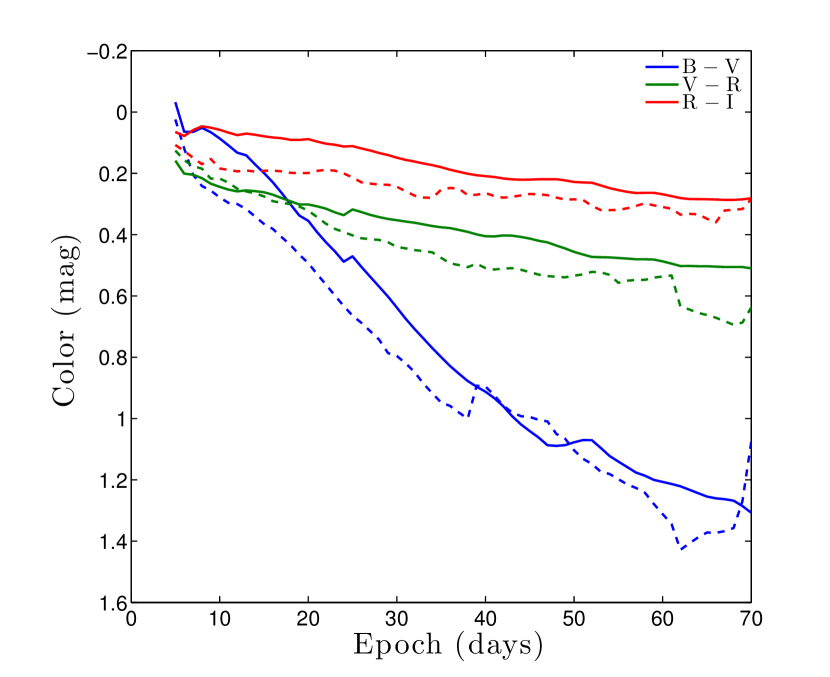
Figure 3: Comparison between the mean colour evolution (averaged over different events) of SNe II-P (solid line) and SNe II-L (dashed line). The two subtypes evolve similarly in all bands, though SNe II-L are redder on average than SNe II-P.

We produce median light curves (in 4 bands, as opposed to the R-band only templates in Li et al. 2011) for the two SN subtypes as follows. Every SN, in every band, was offset in magnitude, so as to minimise scatter before day 50 for a given SN subtype. We then interpolate the light curves linearly in time and calculate the median and median absolute deviation using all available objects. This gives reasonably tight results before day 60 for SNe II-L and day 150 for SNe II-P. The templates are then offset to peak at magnitude zero in $B$ and have at peak the colours we find above. The result can be seen in Figure 4 and is downloadable from http://www.astro.tau.ac.il/~dovip/IIPIIL_templates.txt.

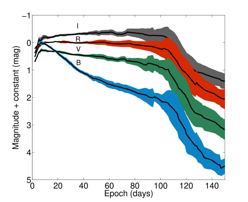
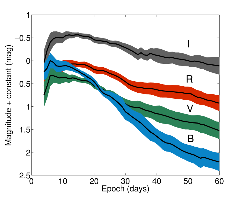
Figure 4: Template SN II-P (top) and SN II-L (bottom) light curves produced using our sample. The curves are offset to have zero $B$-band magnitude at peak and the colours found in Section 3.

3.1 SN II-P – II-L – IIb – A Continuum?

SNe II-P go through a prolonged phase of hydrogen recombination in the envelope, forming a plateau-shaped light curve followed by a sharp decline to the nebular phase. SNe of Type II-L, on the other hand, decline linearly (in magnitudes) after reaching their luminosity peak, $\sim 10$ days after the explosion. The lack of a plateau could suggest that the progenitor has shed a large fraction of its mass before the explosion, so that at the end of its life it has a low-mass hydrogen envelope which cannot sustain a long recombination phase. One could therefore expect a continuum of plateau durations and decline rates, corresponding to different envelope masses.

Based on a sample of 15 SNe II, Arcavi et al. (2012) suggested that there is a clear photometric division of the various SNe II into 3 subclasses rather than a continuum of light-curve shapes. This may indicate that Type II-P, II-L, and IIb events result from distinct progenitor systems (instead of, for example, a one-dimensional mass sequence) such that some thresholds (in binarity or metallicity) guide the stellar evolution into different regimes. More recently, Anderson et al. (2014) and Sanders et al. (2014) published two large samples of SNe II and find that there is no clear gap in the distributions, that there is no obvious photometric threshold that separates the SNe II-P from the SNe II-L.

In order to test that picture, we repeat the process done by Arcavi et al. (2012). Our SN II-L and SN II-P light curves in $V$, $R$, and $I$ are plotted in Figure 5. SNe II-L are shifted to have the same peak magnitude, while SNe II-P are shifted by the average plateau magnitude in the $I$ band during the first 50 days after explosion. This method introduces a bias, since in effect we are assigning the classes before we plot the light curves. However, this would only influence the appearance of the division, as we measure decline self consistently for all SNe. Since it is hard to define a plateau in the $B$ band for SNe II-P, we exclude this band from the analysis.

Our results partly reproduce the findings of Arcavi et al. (2012), who did the same analysis with the $R$-band photometry of 15 SNe II. In all bands the plateau and declining curves do not form a continuum but cluster into two clearly separated subclasses. As discussed by F14a, the SNe II-P show a uniformity of plateau durations of $\sim 100$ days, while SNe II-L span a range of decline rates.

However, in figures 6 and 7 we show the distribution in decline rates in bands $V$ and $I$ respectively, of our SN II-P and SN II-L samples. Clearly, now the classes are not trivial to separate, showing that the methodology of Arcavi et al. (2012) was indeed introducing a bias. Nevertheless, while our small sample is unimodal, it has a long tail which is no very characteristic of a single population (the decline rate values are given in Table LABEL:t:data). We add to this plot the decline rate values calculated by Anderson et al. (2014) for a large sample of SNe. Anderson et al. (2014) defined the parameter ‘$s2$’ to account for the decline rate of the light curve during the recombination period, following the early bump. This definition is similar, though not identical, to the decline rate values of the plateau presented in this plot. The maximum of our distribution falls between the two peaks of Anderson et al. (2014)’s sample. However, The decline rate distribution of the SNe from Anderson et al. (2014) peaks around 0.55 mag$/50$ d, a value we would consider rather II-L-like. Their distribution actually seems bimodal, with a large fraction of SNe with no significant decline, and another with a broad range of decline rates, though this may be sensitive to binning.

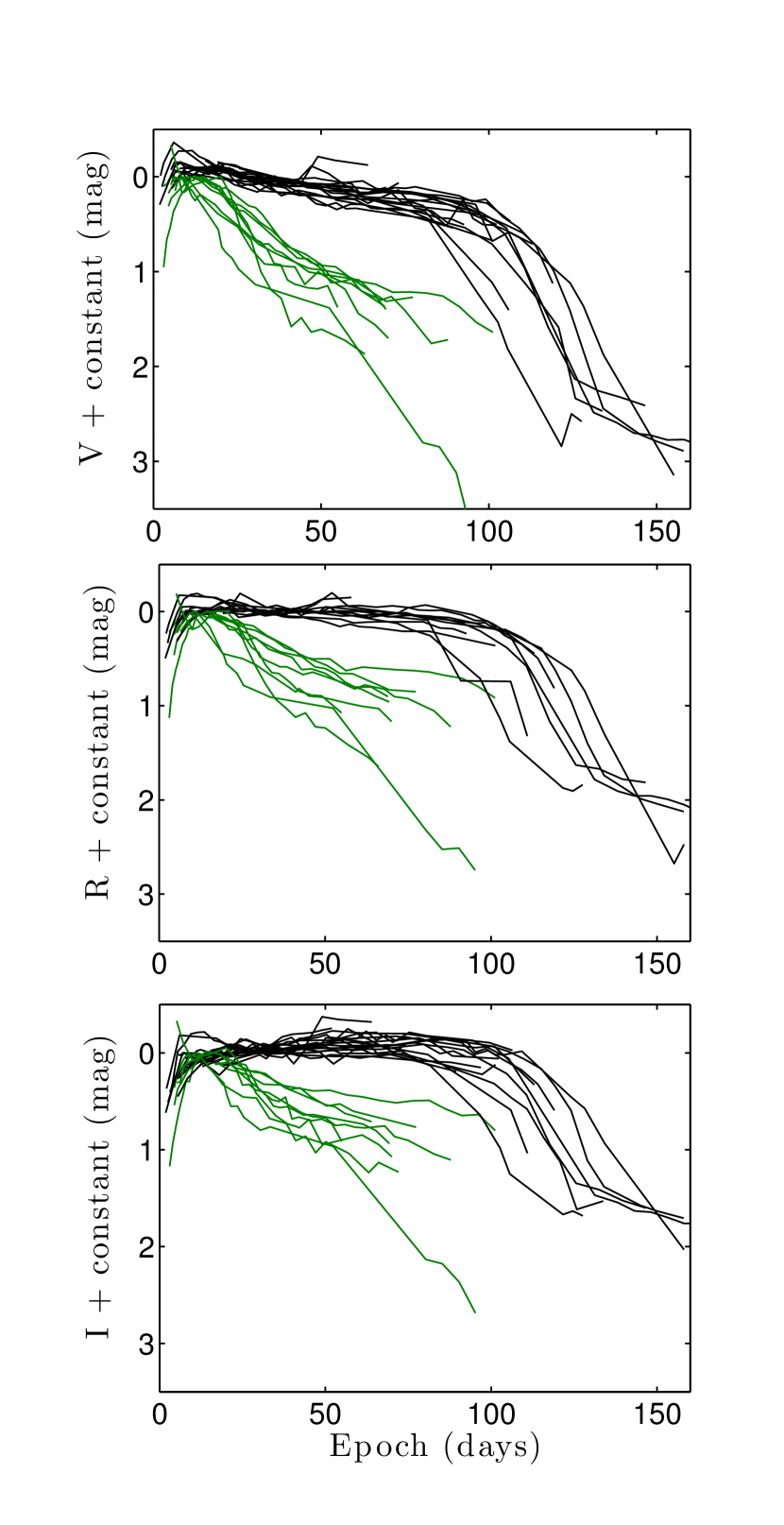
Figure 5: Shifted light curves of all events in the $BVRI$ bands. The curves are visually classified into two subclasses according to the shape of their light curves: SNe II-P (black curves) and linearly declining SNe II-L (green curves). The subclasses seem to be clearly separated by a gap in the $V$, $R$, and $I$ bands.

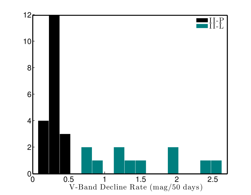
Figure 6: $V$-band decline distribution. We define as SNe II-P (in black) those that decline by less than 0.5 mag from peak brightness in the first 50 days after explosion. Faster decliners are the SNe II-L (shown in green).

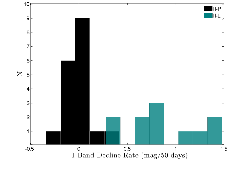
Figure 7: $I$-band decline distribution. Classification is based on the decline in V-band (see figure 6).

To compare the SN II-L subclass to SNe IIb, we compare our light curves with those of the classic Type IIb SN 1993J (data taken from Richmond et al. 1994). Aside from its late rise to peak brightness, this SN IIb seems to resemble some of the SNe II-L (e.g., SNe 2007fz and 2001fa) in its general shape and decline rate. This similarity is apparent in Figure 8, where we set the $R$-band maximum of the SNe II-L to day zero (all events except SN 2001cy and SN 2008es have data at peak brightness). We choose this reference day owing to the variations in rise time. Relative to this reference point, it is clear that SN 1993J is merely a continuation of the SN II-L subclass, for which it serves as a lower bound with the highest decline rate. This behaviour is consistent in the $V$ and $I$ bands as well. This is contrary to the indications found by Arcavi et al. (2012) that the SN IIb light curves are well separated from those of SNe II-L.

One should wonder whether our sample is indeed clearly free of SNe IIb. The light curves of SN 2007fz and SN 2001fa bear a striking resemblance to that of SN 1993J; indeed, SN 2007fz even shows the initial decline and rise to peak magnitude. We examine and mostly reject this hypothesis in Section 4, where we show that all our SNe seem to be more spectroscopically consistent with SNe II-L rather than with SNe IIb.

SNe II-L seem to form a photometric class that might be distinct from SNe II-P, but similar to SNe IIb during their decline. Since the rise time is in effect a tracer of the radius of the star when exploding, while the later parts of the light curve probe the physics of the expanded ejecta, this may indicate that SNe IIb and SNe II-L come from different progenitor channels, but both have been stripped of a significant fraction of their hydrogen via some (perhaps different) mechanism. As we show below, spectroscopy further supports this scenario.

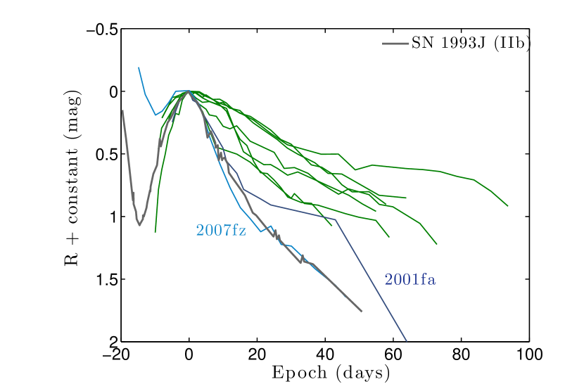
Figure 8: $R$-band photometry of SNe II-L, with the Type IIb SN 1993J for comparison. The light curves are aligned in magnitude and in time by their rise time to peak luminosity. Photometrically, the SN IIb and SN II-L subclasses seem to form a continuum.

4 Spectroscopic Properties

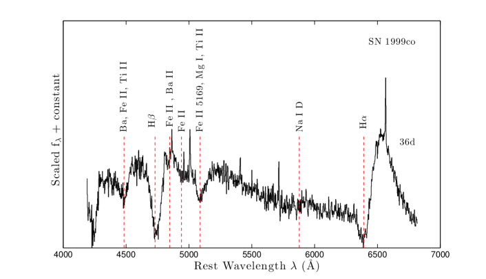
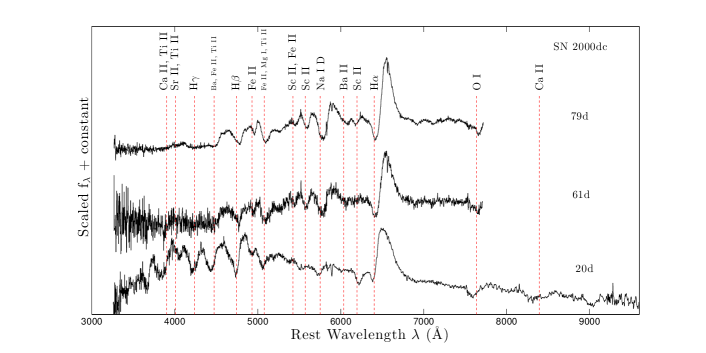
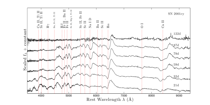
Figure 9: Spectra of SNe 1999co, 2000dc, and 2001cy. Spectral lines appear underdeveloped during early epochs, compared to typical SNe II-P, and show distinct features only starting 20–30 days after explosion. The spectra also seem to lack strong absorption of hydrogen, particularly H$\alpha$. Metal lines are stronger compared to H$\alpha$, evident in the absorption profiles of O I $\lambda$7774 and Na I D/He I $\lambda$5876.

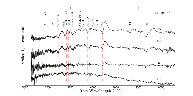
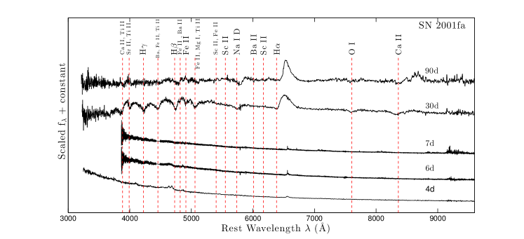
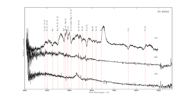
Figure 10: Same as Figure 9 for SNe 2001do, 2001fa, and 2003hf.

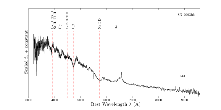
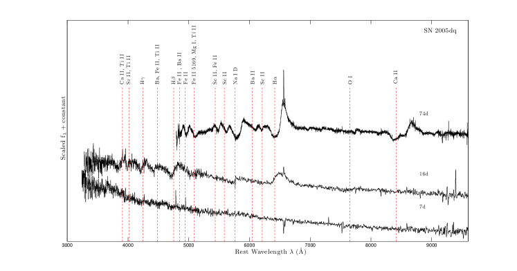
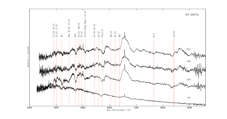
Figure 11: Same as Figure 9 for SNe 2003hk, 2005dq, and 2007fz.

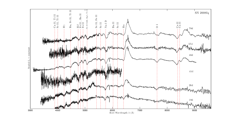
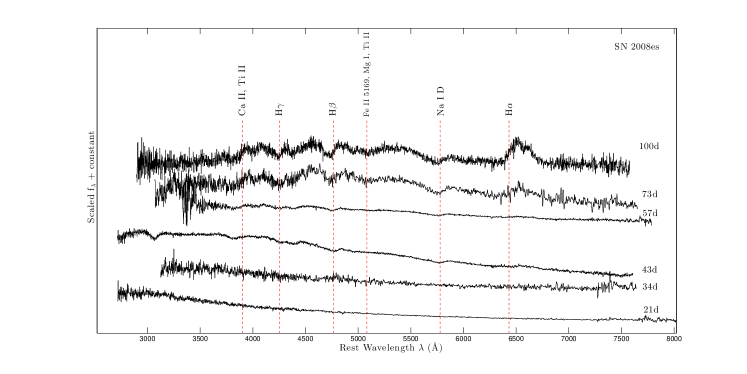
Figure 12: Same as Figure 9 for SNe 2008fq and 2008es.

Figures 9–12 show optical spectra of all SNe II-L in our sample, with spectral lines identified by using the synthetic spectra from Hatano et al. (1999), as described in detail by F14a.

In contrast with standard SN II-P spectra, in SN II-L spectra the hydrogen lines only typically begin to appear at later epochs and are usually weaker than in SNe II-P, as would be expected for hydrogen-poor envelopes.

SN 2001fa, for example, has very few features during its first 9 days. The spectrum on day 30 contains H$\alpha$ in emission, yet with very little absorption, and a much stronger H$\beta$ line. SN 2003hf displays no features at all at day 16, except for a strange emission feature (possibly an artifact?) near 5350 Å, which then almost disappears in the subsequent spectrum on day 22 (see more below). There is no sign whatsoever of hydrogen in the spectra in the first three weeks, and on day 47 we do see strong H$\alpha$ emission but no absorption. Most other objects seem to behave in a similar fashion.

The early-time spectra of SNe 2001fa and 2007fz have narrow H$\alpha$ emission lines, perhaps from circumstellar interaction, but SN 2001fa also shows the C III and N III lines recently identified by Gal-Yam et al. (2014) as being emitted from the outer envelope of the dying star, before it is destroyed by the ejecta. These signs disappear very early in the evolution of the SN, making it hard to determine whether they are present only in the spectra of those two rapidly declining objects or in the rest of the Type II-L subsample as well, for which we do not have such early-time spectra. The emission feature in the first spectrum of SN 2003hf is probably too blue to be He II 5411 Å as in SN 2013cu (Gal-Yam et al. 2014).

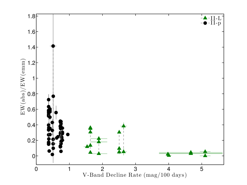
Figure 15: The EW ratios of H$\alpha$ absorption to emission. Dashed lines connect multiple spectra of the same SN. These ratios are typically larger in spectra of SNe II-P, confirming the suggestion of Schlegel (1996) and the recent results of Gutiérrez et al. (2014).

Schlegel (1996) suggested that SNe II-L have typically shallower H$\alpha$ absorption compared to emission, while SNe II-P have deeper P-Cygni absorption profiles. In Figure 15 we confirm this idea, as also recently shown by Gutiérrez et al. (2014). The data used in this figure are presented in Table LABEL:t:Ha.

Table 5: ${\rm H\alpha}$ Properties

SN Name	Age (days)	EWHα (abs)/EWHα (emm)
1999bg	41.0	0.01(0.25)
1999co	36.5	0.02(0.12)
1999em	11.4	0.01(0.17)
1999em	13.4	0.02(0.17)
1999em	14.7	0.01(0.15)
1999em	15.7	0.01(0.15)
1999em	25.4	0.03(0.27)
1999em	28.4	0.03(0.33)
1999em	30.3	0.07(0.72)
1999em	34.3	0.02(0.40)
1999em	38.3	0.03(0.53)
1999em	41.6	0.02(0.51)
1999em	44.1	0.01(0.63)
1999em	48.3	0.02(0.59)
1999em	51.3	0.03(0.55)
1999em	53.1	0.01(0.58)
1999gi	29.8	0.02(0.29)
1999gi	34.8	0.02(0.38)
1999gi	37.8	0.02(0.44)
2000bs	74.3	0.09(0.56)
2000dc	20.4	0.00(0.03)
2000dc	61.4	0.03(0.18)
2000dc	79.3	0.03(0.22)
2000dj	25.0	0.02(0.23)
2000dj	35.1	0.05(0.24)
2000dj	53.0	0.02(0.24)
2000dj	61.0	0.02(0.20)
2001bq	55.4	0.06(0.33)
2001bq	72.4	0.05(0.43)
2001bq	20.2	0.00(0.02)
2001cm	26.3	0.03(0.12)
2001cm	43.3	0.04(0.27)
2001cm	54.2	0.02(0.30)
2001cm	81.1	0.02(0.35)
2001cy	21.5	0.01(0.04)
2001cy	32.4	0.01(0.13)
2001cy	59.4	0.03(0.31)
2001cy	79.2	0.03(0.36)
2001cy	87.3	0.03(0.35)
2001do	11.2	0.03(0.05)
2001do	30.0	0.02(0.05)
2001do	31.0	0.02(0.09)
2001do	39.1	0.02(0.30)
2001fa	30.5	0.01(0.02)
2001x	26.8	0.02(0.27)
2001x	34.3	0.01(0.60)
2001x	35.9	0.01(0.35)
2001x	52.3	0.01(0.57)
2001x	66.7	0.02(0.59)
2001x	82.7	0.04(0.50)
2002ca	19.2	0.04(0.20)
2002ca	31.6	0.05(0.36)
2002ca	48.6	0.05(0.31)
2002ca	89.4	0.02(0.29)
2002gd	24.8	1.50(1.41)
2002gd	50.0	0.01(0.16)
2002gd	31.8	0.02(0.21)
2002hh	44.3	0.03(0.23)
2003hf	46.8	0.01(0.00)
2003hl	12.4	0.01(0.06)
2003hl	73.3	0.02(0.41)
2003hl	68.0	0.02(0.44)
2003iq	20.8	0.01(0.19)
2003iq	46.8	0.01(0.36)
2003iq	15.5	0.01(0.16)
2003z	10.1	0.01(0.06)
2004du	44.5	0.02(0.28)
2004et	19.6	0.01(0.13)
2004et	20.7	0.00(0.12)
2004et	57.6	0.00(0.45)
2004et	57.6	0.02(0.38)
2004et	80.7	0.00(0.44)
2004et	52.0	0.02(0.38)
2005ay	29.3	0.02(0.22)
2005ay	35.1	0.02(0.34)
2005ay	35.1	0.02(0.34)
2005ay	35.1	0.01(0.36)
2005ay	63.2	0.04(0.56)
2005cs	16.0	0.00(0.10)
2005cs	38.0	0.02(0.77)
2005dq	12.3	0.04(0.05)
2005dq	73.9	0.05(0.38)
2007fz	23.1	0.01(0.05)
2007fz	29.9	0.01(0.00)
2008fq	46.4	0.00(0.03)
2008fq	57.2	0.01(0.04)
2008fq	70.2	0.01(0.03)

H$\beta$ absorption is stronger than H$\alpha$ absorption, but much weaker than in SNe II-P. Metal lines that we identified in the spectra of SNe II-P are also present here, and appear a bit stronger (see, e.g., O I $\lambda$7774) and are generally more prominent than H$\alpha$. The strong metal lines are a consequence of the high density at the photosphere expected for a rapid recombination wave. The Na I D line appears wider than its counterpart in SN II-P spectra, suggesting either a larger velocity dispersion, or perhaps more likely, a greater contribution from the He I $\lambda$5876 line.

The superluminous SN 2008es is exceptional in that it shows no features at all through day 34 after explosion. The spectrum on day 73 is more developed, but with no clear H$\alpha$ absorption. Miller et al. (2009) also note the lack of features during early epochs, and the absence of H$\alpha$ absorption is supported by their additional spectra. They suggest that the muted amplitude of the spectral features can be explained through the “top-lighting effect” described by Branch et al. (2000). This effect rescales the amplitude of the lines by illumination from continuum emission that originates from interaction with the circumstellar medium.

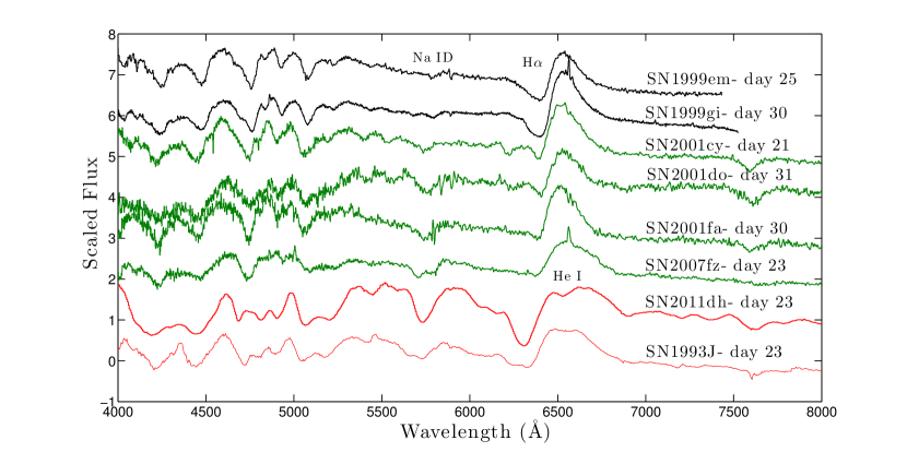
Figure 13: Spectroscopic comparison between SNe II-P, II-L, and IIb around days 20–30. Surprisingly, the Type IIb SN 2011dh has a strong H$\alpha$ absorption that is equivalent to (if not stronger than) that in both SNe II-P. The He I/Na I D line behaves as expected, gradually increasing in strength as we go from SNe II-P to IIb, owing to higher helium abundance in SNe II-L and IIb. An interesting feature is the additional absorption dip seen in the H$\alpha$ P-Cygni emission component of both SNe IIb, which is absent in spectra of SNe II-L and II-P. This feature can probably be associated with He I $\lambda$6678. Also evident is the wider P-Cygni emission in spectra of SNe IIb than in SNe II-P or II-L.

In Section 3.1 we point out the photometric resemblance of SNe 2007fz and 2001fa to typical SNe IIb. This raised the suspicion that they were misclassified SNe IIb. We compare their spectra (days 23 and 30) to spectra of SNe II-P and II-L from our joint sample at similar epochs, and to two SNe IIb (SN 1993J and 2011dh). Clear differences are evident among the three classes in Figure 13. Since SNe II-L have weaker H$\alpha$ absorption compared with SNe II-P, one could expect SNe IIb to have even weaker hydrogen lines. Surprisingly, though, the opposite is true: SN 2011dh has strong H$\alpha$ absorption that is equivalent to (if not stronger than) that in both SNe II-P. The H$\alpha$ line in SN 1993J is weaker than in SN 2011dh, but still at least as strong as those of the SNe II-L. The He I/Na I D line behaves as expected, gradually increasing in strength as we go from SNe II-P to IIb, probably due to higher helium abundance.

The most distinctive difference, however, is probably the additional absorption dip seen in the H$\alpha$ P-Cygni emission component, appearing in both of the SNe IIb but in none of the SNe II-L or II-P. This feature can probably be associated with He I line at 6678 Å. The P-Cygni emission also appears somewhat broader in both SNe IIb (and also slightly in SN 2007fz), pointing to a large velocity dispersion. The spectra of SNe 2007fz and 2001fa (particularly at later phases) show more resemblance to the spectra of the other SNe II-L than to those of SNe IIb.

However, what if SNe 2007fz or 2003hk, for which we only have early-time spectra, later evolved to show no hydrogen, and therefore retroactively became SNe IIb? This might be a purely semantic question, since the diversity of progenitor systems and SN characteristic do not allow one to draw any direct conclusion from such a transition or lack thereof. More objects, with better sampling of the spectroscopic evolution, is required to answer that question and better understand how much the photometric and spectroscopic classes overlap.

4.1 He Abundance Tracers

If indeed SNe II-L come from massive stars with thin hydrogen envelopes, and helium contributes to the different light-curve shapes, we should see clear signs of this in the spectra as well. The strongest helium line — He I line at 5876 Å — is unfortunately blended with Na I D $\lambda$5896. Other helium lines in our spectral range are too weak and usually absent. We must therefore use a proxy for a helium-rich composition.

The two scenarios of hydrogen-rich and helium-rich envelopes are addressed in detail by Hatano et al. (1999), who calculated the local thermodynamic equilibrium (LTE) optical depths of the most probable ions in the Sobolev approximation as a function of temperature. The hydrogen-rich scenario describes a typical SN II-P with a large hydrogen envelope, while the helium-rich composition represents the stripped SNe of Type Ib. A somewhat intermediate composition would be achieved in progenitors which have not lost their entire outer hydrogen envelope, but are still hydrogen deficient. In such a case, the He I and He II lines should become stronger owing to the high abundance of helium. Likewise, metal lines become more prominent as a result of the increasing density near the photosphere. From Hatano et al. (1999) we find that O I is the only ion in our spectral range (apart from helium ions) that becomes more prominent when transitioning from a H-rich to a He-rich atmosphere.

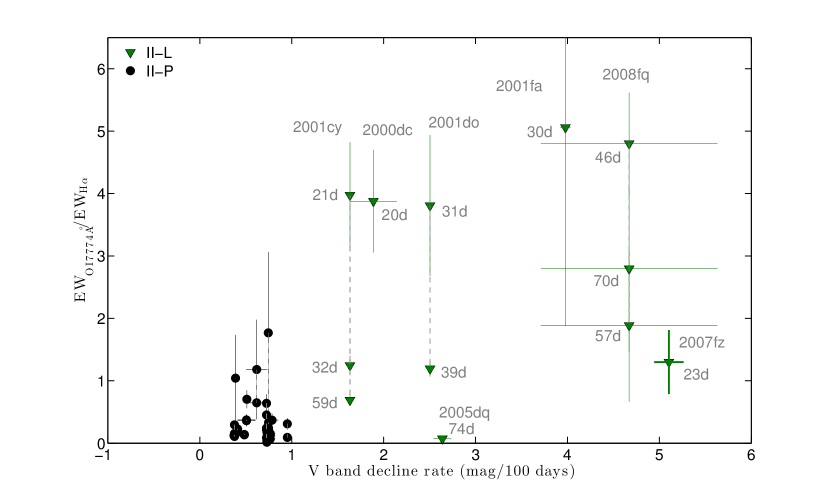
Figure 14: The EW ratios of H$\alpha$ and O I $\lambda$7774 vs. the $V$-band decline rate. We indicate the epoch at which the EWs are measured for the SNe II-L. Dashed lines connect multiple spectra of a same SN. One can see a correlation between decline rate and the relative strength of the O I $\lambda$7774 line.

We measure the equivalent width (EW) of the absorption component of O I $\lambda$7774 for our sample, and scale it by the EW of H$\alpha$ in order to get a handle on the relative abundance. Both H$\alpha$ and O I $\lambda$7774 are isolated lines, between which the continuum is roughly flat and hardly varies. If our above analysis is correct, then SNe II-L (and generally objects with declining light curves) should have stronger O I to H$\alpha$ ratios. In Figure 14 we show this ratio as a function of the $V$-band decline per 100 days. SNe II-L typically have a higher ratio, and it weakens with time owing to the increasing strength of H$\alpha$. The data used for this figure are presented in Table LABEL:t:EW_HO.

Table 6: ${\rm H\alpha}$ vs. O I 7774 Å

SN Name	Age (days)	EW(H$\rm\alpha$)/EW(O I 7774 Å)
1999d	19.7	0.52(0.20)
1999em	41.6	0.12(0.01)
1999gi	34.8	0.04(0.01)
1999gi	37.8	0.02(0.01)
2000dc	20.4	3.88(0.82)
2000dj	25.0	0.07(0.02)
2000dj	35.1	0.13(0.07)
2000dj	53.0	0.15(0.04)
2001bq	55.4	0.14(0.07)
2001bq	72.4	0.13(0.03)
2001cm	81.1	0.10(0.02)
2001cm	109.0	0.17(0.02)
2001cy	21.5	3.97(0.85)
2001cy	32.4	1.25(0.16)
2001cy	59.4	0.69(0.09)
2001do	31.0	3.81(1.13)
2001do	39.1	1.19(0.13)
2001fa	30.5	5.06(3.18)
2001hg	35.1	0.15(0.06)
2001hg	79.1	0.10(0.03)
2001hg	40.5	0.15(0.04)
2001x	26.8	0.23(0.03)
2001x	35.9	0.18(0.02)
2002an	28.1	2.73(1.35)
2002an	31.2	2.18(0.34)
2002an	56.0	1.06(0.20)
2002bx	30.1	0.56(0.14)
2002bx	30.1	0.55(0.13)
2002bx	47.0	0.19(0.06)
2002bx	59.0	0.19(0.04)
2002ca	31.6	0.37(0.11)
2002gd	50.0	0.36(0.09)
2002gd	31.8	0.37(0.09)
2002hh	4.3	1.18(0.80)
2002hh	44.3	0.65(0.13)
2003gd	85.0	0.07(0.01)
2003gd	92.9	0.10(0.02)
2003hl	12.4	1.77(1.30)
2003hl	68.0	0.15(0.02)
2003iq	20.8	0.33(0.07)
2003iq	46.8	0.20(0.02)
2003iq	15.5	0.24(0.07)
2003z	10.1	1.04(0.69)
2004du	44.5	0.31(0.09)
2004du	100.3	0.09(0.02)
2004et	19.6	0.64(0.14)
2004et	20.7	0.45(0.06)
2004et	57.6	0.23(0.01)
2004et	57.6	0.21(0.02)
2004et	80.7	0.08(0.01)
2004et	52.0	0.24(0.02)
2005ay	29.3	0.29(0.05)
2005ay	35.1	0.16(0.03)
2005ay	63.2	0.11(0.01)
2005cs	16.0	0.70(0.14)
2005dq	73.9	0.07(0.03)
2007fz	23.1	1.30(0.51)
2008fq	46.4	4.80(0.82)
2008fq	57.2	1.89(1.22)
2008fq	70.2	2.80(1.33)

5 Velocity Evolution

We measure the H$\alpha$ and H$\beta$ velocities, along with the photospheric velocities from the minimum of the Fe II $\lambda$5169 line. The measurements and their uncertainties are obtained as described by F14a. We find that the photospheric velocities of the SNe II-L are generally higher than those of the SNe II-P throughout their evolution. However, the velocities of the SN II-L hydrogen lines start off lower, but after $\sim 50$ days they surpass the velocities of the SNe II-P, which seem to decline faster over time.

In Figure 16 we show the velocities of the three lines as a function of time, scaled by the velocity on day 50. We also plot the power laws obtained for the sample of 23 SNe II-P by F14a. It is clear that the hydrogen velocities, especially H$\beta$, do not follow the same power law as the SNe II-P at early epochs, and the time dependence of their velocities is quite weak.

This can be explained as follows. As the photosphere recedes inward, it reveals hydrogen-poor layers. Therefore, the absorption comes mostly from external (and faster) layers, and not from the photosphere. As a consequence, unlike in SNe II-P during the plateau phase, the time dependence does not result from inner and slower layers being exposed. A similar process occurs for SNe II-P at later times. The iron line, however, which (at least in SNe II-P) might be a better tracer of the photosphere, does seem to generally follow the power law derived from SNe II-P, albeit with significant scatter.

6 Conclusions

In this work we analyze a sample of 11 SNe II-L, one of the largest such samples ever studied. We define this subclass as being those SNe II having a $V$-band light curve that declines from peak brightness by more than 0.5 mag in the first 50 days. We demonstrate that SNe II-L have a spectroscopic evolution that is mostly distinct from other SN types. This however does not argue against the photometric continuum that Anderson et al. (2014) and Sanders et al. (2014) find between SNe II-P and II-L. Furthermore, it seems that photometrically, SNe II-L are closely related to SNe IIb.

In addition to their more rapid photometric decline and higher peak luminosities (by about 1.5 mag), we identify three spectroscopic characteristics that are common to most SNe II-L, as follows.

• SNe II-L typically have few features and comparatively weak hydrogen absorption lines throughout most of their lifetimes, as well as a larger ratio of H$\alpha$ emission to absorption than SNe II-P (Schlegel 1996; Gutiérrez et al. 2014).

• Strong O I $\lambda$7774 absorption relative to H$\alpha$ at early times, compared with SNe II-P. It seems that if caught within $\sim 3$ weeks past maximum brightness, the ratio is $>1.0$, whereas for SNe II-P it is $<1.0$. Using the O I $\lambda$7774 line as a proxy for a helium-rich envelope, we find that the helium abundance correlates with the photometric decline rate, and that indeed SNe II-L are more helium rich, and hence hydrogen poor.

• More slowly evolving H$\beta$ velocity. In particular, SN II-P velocities decrease from maximum light relative to day 50 by a factor of 3, whereas SN II-L velocities generally drop by $\lesssim 50$%. This is expected if the line is formed in the outer layers of the ejecta rather than in a thick, gradually exposed, hydrogen envelope.

All of these characteristics might suggest that SNe II-L come from progenitors that are poorer in hydrogen than those of SNe II-P. Along with their possible tendency to suffer from more dust extinction, this trend can be possibly explained if SNe II-L come from stars with initial masses higher than $\sim 15$ M_⊙.

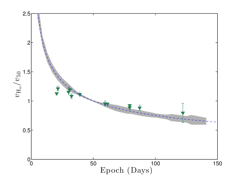
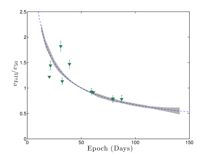
Figure 16: H$\alpha$ (top-left panel), H$\beta$ (top-right), and Fe II $\lambda$5169 (bottom) velocities normalised by $v_{50}$, the velocity on day 50. The dashed line is the power law found by F14a for a sample of 23 SNe II-P, and the shaded area represents the mean distance of the SN II-P velocities from this line. One can see that the hydrogen velocities do not follow the power law. However, the Fe II measurements show a similar evolution with significant scatter.

References

- Anderson et al. (2014) Anderson J. P. et al., 2014, ArXiv:1403.7091
- Arcavi et al. (2012) Arcavi I. et al., 2012, ApJ, 756, L30
- Arnett (1996) Arnett D., 1996, Supernovae and Nucleosynthesis, Ostiker J. P., ed. New Jersey: Princeton University Press
- Bayless et al. (2014) Bayless A. J., Even W., Frey L. H., Fryer C. L., Roming P. W. A., Young P. A., 2014, ArXiv e-prints
- Branch et al. (1981) Branch D., Falk S. W., Uomoto A. K., Wills B. J., McCall M. L., Rybski P., 1981, ApJ, 244, 780
- Branch et al. (2000) Branch D., Jeffery D. J., Blaylock M., Hatano K., 2000, PASP, 112, 217
- Elias-Rosa et al. (2010) Elias-Rosa N. et al., 2010, ApJ, 714, L254
- Faran (2014) Faran T. e. a., 2014, ArXiv
- Filippenko (1997) Filippenko A. V., 1997, ARA&A, 35, 309
- Fraser et al. (2010) Fraser M., Takats K., Pastorello A., Smartt S. J., Mattila S., Botticella M.-T., 2010, ApJ, 714, L280
- Gal-Yam et al. (2014) Gal-Yam A. et al., 2014, Nature, 509, 471
- Gezari et al. (2009) Gezari S. et al., 2009, ApJ, 690, 1313
- Gutiérrez et al. (2014) Gutiérrez C. P. et al., 2014, ArXiv:1403.7089
- Hatano et al. (1999) Hatano K., Branch D., Fisher A., Millard J., Baron E., 1999, ApJS, 121, 233
- Kasen & Woosley (2009) Kasen D., Woosley S. E., 2009, ApJ, 703, 2205
- Kleiser et al. (2011) Kleiser I. K. W. et al., 2011, MNRAS, 415, 372
- Kochanek (2013) Kochanek C. S., 2013, ArXiv e-prints
- Li et al. (2011) Li W. et al., 2011, MNRAS, 412, 1441
- Miller et al. (2009) Miller A. A. et al., 2009, ApJ, 690, 1303
- Özel et al. (2010) Özel F., Psaltis D., Narayan R., McClintock J. E., 2010, ApJ, 725, 1918
- Özel et al. (2012) Özel F., Psaltis D., Narayan R., Santos Villarreal A., 2012, ApJ, 757, 55
- Patat et al. (1994) Patat F., Barbon R., Cappellaro E., Turatto M., 1994, A&A, 282, 731
- Popov (1993) Popov D. V., 1993, ApJ, 414, 712
- Poznanski (2013) Poznanski D., 2013, MNRAS, 436, 3224
- Poznanski et al. (2009) Poznanski D. et al., 2009, ApJ, 694, 1067
- Poznanski et al. (2011) Poznanski D., Ganeshalingam M., Silverman J. M., Filippenko A. V., 2011, MNRAS, 415, L81
- Poznanski, Prochaska & Bloom (2012) Poznanski D., Prochaska J. X., Bloom J. S., 2012, MNRAS, 426, 1465
- Richmond et al. (1994) Richmond M. W., Treffers R. R., Filippenko A. V., Paik Y., Leibundgut B., Schulman E., Cox C. V., 1994, AJ, 107, 1022
- Sanders et al. (2014) Sanders N. E., Soderberg A. M., Gezari S., Betancourt M., Chornock R., Berger E., Foley R. J., Challis P., 2014, ArXiv: 1404.2004
- Schlegel, Finkbeiner & Davis (1998) Schlegel D. J., Finkbeiner D. P., Davis M., 1998, ApJ, 500, 525
- Schlegel (1996) Schlegel E. M., 1996, AJ, 111, 1660
- Silverman et al. (2012) Silverman J. M., Foley R. J., Filippenko A. V., Ganeshalingam M., Barth A. J., Chornock R., 2012, MNRAS, 425, 1789
- Smartt (2009) Smartt S. J., 2009, ARA&A, 47, 63
- Smith et al. (2011) Smith N., Li W., Filippenko A. V., Chornock R., 2011, MNRAS, 412, 1522
- Thompson (1982) Thompson L. A., 1982, ApJ, 257, L63
- Turatto, Benetti & Cappellaro (2003) Turatto M., Benetti S., Cappellaro E., 2003, in From Twilight to Highlight: The Physics of Supernovae, Hillebrandt W., Leibundgut B., eds., p. 200
- Uomoto & Kirshner (1986) Uomoto A., Kirshner R. P., 1986, ApJ, 308, 685
- Van Dyk et al. (1999) Van Dyk S. D. et al., 1999, PASP, 111, 313
- Yaron & Gal-Yam (2012) Yaron O., Gal-Yam A., 2012, PASP, 124, 668