A critical assessment of some inhomogeneous pressure Stephani models

Abstract

We consider spherically symmetric inhomogeneous pressure Stephani universes, the center of symmetrybeing our location. The main feature of these models is that comoving observers do not follow geodesics. In particular, comoving perfect fluids have necessarily a radially dependent pressure. We consider a subclass of these models characterized by some inhomogeneity parameter $\beta$. We show that also the velocity of sound, like the (effective) equation of state parameter, of comoving perfect fluids acquire away from the origin a time and radial dependent change proportional to $\beta$. In order to produce a realistic universe accelerating at late times without dark energy component one must take $\beta<0$. The redshift gets a modified dependence on the scale factor $a(t)$ with a relative modification of $-9\%$ peaking at $z\sim 4$ and vanishing at the big-bang and today on our past lightcone. The equation of state parameter and the speed of sound of dustlike matter (corresponding to a vanishing pressure at the center of symmetry $r=0$) behave in a similar way and away from the center of symmetry they become negative – a property usually encountered for the dark energy component only. In order to mimic the observed late-time accelerated expansion, the matter component must significantly depart from standard dust, presumably ruling this subclass of Stephani models out as a realistic cosmology. The only way to accept these models is to keep all standard matter components of the universe including dark energy and take an inhomogeneity parameter $\beta$ small enough.

I Introduction

One of the ways to solve the dark energy problem DE is to consider non-uniform models of the Universe which could explain the acceleration only due to inhomogeneity UCETolman ; center . There is a suggestion that we live in a spherically symmetric void of density described by the Lemaître-Tolman-Bondi (LTB) concentric dust spheres model LTB . The simplest inhomogeneous cosmological models are spherically symmetric of which category LTB models are complementary to Stephani models stephani ; dabrowski93 ; dabrowski95 . The former have inhomogeneous density $\varrho(t,r)$ (variable density dust shells) while the latter have inhomogeneous pressure $p(t,r)$ (variable pressure shells).

In view of large expansion of investigations related to LTB models as nearly the only example of an inhomogeneous cosmology, we think that it is useful to fully consider a theoretical basis and observational validity of the complementary Stephani universes. The number of papers about these models is tight in comparison to LTB models. In this paper we would like to fill in this gap slightly. One of the benefits of Stephani cosmology is that it possesses a totally spacetime inhomogeneous generalization stephani ; dabrowski93 which is not the case for LTB models and for example for Barnes models barnes73 which belong to the same class of shear-free, irrotational, expanding (or collapsing) perfect fluid models as Stephani models (the so-called Stephani-Barnes family). This property is of course a good step towards developing more models of such a type - i.e. the universes which describe real inhomogeneity of space (for a review see e.g. Ref. krasinski ; BKC ) - not only those, which possess rather unrealistic center of the Universe - something which is against the Copernican principle. This challenge requires the proper comparison of very general inhomogeneous models with data which was first ever done for Stephani models in Ref. dabrowski98 and for LTB models in Ref. LTBtests .

In general, there is a lot of inhomogeneous models which are exact solutions of the Einstein field equations and not just the perturbations of the isotropic and homogeneous Friedmann cosmology. Curiously, observations are practically made from just one point in the Universe (apart from the redshift drift sandage ; loeb ) and extend only onto the unique past light cone of the observer placed on the Earth. Even the cosmic microwave background radiation is observed from one point so that its observations prove isotropy of the Universe, but not necessarily its homogeneity chrisroy . As suggested in Ref.ellis one should start with model-independent observations of the past light cone and then make conclusions related to geometry of the Universe, though it is difficult to really differentiate between an inhomogeneous model of the Universe with the same number of parameters as a homogeneous dark energy model when both fit observations.

In Ref.GSS it has been shown that pressure inhomogeneity can mimic dark energy in the sense that they produce the same redshift-magnitude relation. The assumption was that inhomogeneity has dominated the universe quite recently, so it influenced only slightly the Doppler peaks and did not influence big-bang nucleosynthesis at all. This assumption was in agreement with the “definition 1” of the last scattering surface in Ref.chris according to which the homogeneous and isotropic radiation field on this surface was assumed (in our prospective notation this will be equivalent to the statement that the function $V(t,r)\to 1$ at $t\to 0$). Such a property is due to conformal flatness which does not lead to any affect on photon paths which was also discussed recently in Ref.visser . In the context of inhomogeneous pressure, some generalized Ehlers-Geren-Sachs (EGS) theorems were discussed in Ref.chris99 which said that an exactly isotropic radiation field for every fundamental observer was possible despite there was an acceleration of the observers – only when it vanished, the models became Friedmann. In other words, and according to this generalized theorem, high degree of isotropy of the universe (isotropic radiation field) plus Copernican principle did not force it to be homogeneous.

In fact, in Ref.chris a different set of Stephani models has been studied and discussed in the context of cosmic microwave background data. This set was actually defined by Da̧browski in Ref.dabrowski93 by the formulas (43) and (44) (the scale factor and the curvature function) as well as by the formulas (57a) and (57b) (the mass density and the pressure). A subclass of these models was then dubbed Models I in Ref.dabrowski95 and because of the choice of the quantity $\Delta=0$ they offered less freedom in the choice of parameters. A common feature of these two types of models (both with $\Delta=0$ and $\Delta\neq 0$) was that they had a fixed cosmic-string-like equation of state $p=-(1/3)\varrho$ at the center of symmetry. In fact, the Ref.GSS used a version of Models II of Ref. dabrowski95 – the one which allowed the barotropic equation of state at the center of symmetry (Stephani models in general do not have this property) and which are more restrictive. Quite a large generality of the models I (with $\Delta\neq 0$) studied in Ref.chris eased the claim that they can fit the data despite they were significantly inhomogeneous. In Ref.PRD13 which we will further call Paper 1, the effect of redshift drift for the Stephani models II has been studied. The similarities and differences between standard $\Lambda$CDM, LTB and Stephani models which can be tested by the future astronomical data were clearly presented. In Ref.off-center14 Models I with $\Delta=0$ as well as Models II with barotropic equation of state at the center of symmetry were tested by Union2 supernovae data for an off-center (i.e. non-centrally placed) observer and the maximum location of the center with respect to the observer was evaluated in each model.

In this paper, and especially in its observational part where we use the data, we restrict ourselves to the centrally placed observers and discuss Models II with a barotropic equation of state at the center of symmetry only. In Sec.II we present the properties of inhomogeneous pressure Stephani models. In Sec.III we present in details the particular model we will study, emphasizing analogies and important differences with standard cosmological models. In Sec.IV we derive expressions for standard quantities used in order to constrain our model. Sec.IV.1 is devoted to the comparison of our particular Stephani universe with observational data. Finally in Sec.V we summarize our results and give our conclusion.

II Inhomogeneous pressure cosmology

In Paper 1 PRD13 we presented the basic properties of the inhomogeneous pressure Stephani universes and here we give only their most important characteristics. Mathematically, they are the only spherically symmetric solutions of Einstein equations for a perfect-fluid energy-momentum tensor $T^{ab}=(\varrho c^{2}+p)u^{a}u^{b}+pg^{ab}$ ($\varrho$ is the mass density, $p$ is the pressure, $g^{ab}$ is the metric tensor, $u^{a}$ is the 4-velocity vector, $c$ is the velocity of light) which are conformally flat and can be embedded in a five-dimensional flat pseudoeuclidean space stephani ; dabrowski93 . A general model has no spacetime symmetries at all, but in this paper we consider only spherically symmetric Stephani models of which metric reads as

$$ds^{2}=-\frac{a^{2}}{\dot{a}^{2}}\left[\frac{\left(\frac{V}{a}\right)^{\centerdot}}{\left(\frac{V}{a}\right)}\right]^{2}c^{2}dt^{2}~{}+\frac{a^{2}}{V^{2}}\left(dr^{2}~{}+~{}r^{2}d\Omega^{2}\right),$$ (II.1)

where

$$V(t,r)=1+\frac{1}{4}k(t)r^{2}~{},$$ (II.2)

and $(\ldots)^{\centerdot}~{}\equiv~{}\partial/\partial t$. Here $a(t)$ is a generalized scale factor, $r$ is the radial coordinate, $d\Omega$ is the metric on the sphere, and $k(t)$ is a time-dependent curvature index which allows the Universe to “open up” to become negatively curved or to “close down” to become positively curved.

The mass density and the pressure for a comoving perfect fluid are given by

$$\varrho(t) = \frac{3}{8\pi G}\left[\frac{\dot{a}^{2}(t)}{a^{2}(t)}+\frac{k(t)c^{2}}{a^{2}(t)}\right]~{},$$ (II.3)

$$p(t,r) = \left[-1+\frac{1}{3}\frac{\dot{\varrho}(t)}{\varrho(t)}\frac{\left[\frac{V(t,r)}{a(t)}\right]}{\left[\frac{V(t,r)}{a(t)}\right]^{\centerdot}}\right]\varrho(t)c^{2}$$

$$\equiv w_{e}(t,r)\varrho(t)c^{2},$$

where $G$ is the gravitational constant, and $w_{e}(t,r)$ is an effective spatially dependent barotropic index. Of course, one can have more than one (comoving) perfect fluid as it is the case in a realistic cosmology. We will address in great details in Section III a particular class of these models and show the analogy and fundamental differences with standard Friedmann universes. In fact, the Stephani models admit standard big-bang singularities ($a\to 0$, $\varrho\to\infty$, $p\to\infty$), and finite density (FD) singularities of pressure sussmann ; dabrowski93 which resemble sudden future singularities (SFS) barrow04 ; PRD05 of Friedmann cosmology. In LTB models there exist “shell-crossing” singularities shell , which are of a weak type in the sense of Tipler and Królak tipler+krolak and are similar to Friedmannian generalized sudden future singularities (GSFS) GSFS which do not lead to geodesic incompleteness lazkoz ; AIP10 .

For further discussion it is useful to mention that the components of the 4-velocity and the 4-acceleration vectors are dabrowski95

$$u_{t}=-~{}\frac{c}{V}~{},\hskip 22.76228pt\dot{u}_{r}=-c~{}\frac{V_{,r}}{V}~{},$$ (II.5)

and the acceleration scalar reads as

$$\dot{u}~{}\equiv\left(\dot{u}_{a}\dot{u}^{a}\right)^{\frac{1}{2}}~{}=~{}\frac{V_{,r}}{a}~{}.$$ (II.6)

Tangent to a null geodesic vector components are dabrowski95

$$k^{t}=\frac{V^{2}}{a}~{},\hskip 5.69046ptk^{r}=\pm\frac{V^{2}}{a^{2}}\sqrt{1~{}-~{}\frac{h^{2}}{r^{2}}}~{},\hskip 5.69046ptk^{\theta}=0~{},\hskip 5.69046ptk^{\phi}=h\frac{V^{2}}{a^{2}r^{2}}~{},$$ (II.7)

($h$ = const.) – the plus sign applies to a ray moving away from the center of symmetry, the minus sign applies to a ray moving towards the center. The constant $h$ and the angle $\phi$ between the direction of observation and the direction defined by the observer and the center of symmetry are related by

$$\cos{\phi}=\pm\sqrt{1~{}-~{}\frac{h^{2}}{r^{2}}}~{}~{}.$$ (II.8)

The angle $\phi$ should be taken into account when one considers off-center observers dabrowski95 ; off-center14 .

In Ref.dabrowski93 two classes exact spherically symmetric Stephani models were found:

• Models I which fulfill the condition $(V/a)^{\centerdot\centerdot}=0$

• Models II which fulfill the condition $(k/a)^{\centerdot}=0$.

A subclass of Models I dabrowski93 which is not the one used in Ref. chris as well as in Refs.dabrowski95 ; dabrowski98 ) is given by:

$$a(t)=\frac{1}{\gamma t+\delta},\hskip 28.45274ptk(t)=\frac{\alpha t+\sigma}{\gamma t+\delta}~{}~{},$$ (II.9)

with the units of the constants given by: $[\alpha]$ = Mpc s^-1, $[\sigma]$ = Mpc, $[\gamma]$ = Mpc^-1 s^-1, and $[\delta]$ = Mpc^-1. The metric (II.1) takes the form

$$ds^{2}=\frac{a^{2}}{V^{2}}\left[-\left(\frac{a}{\dot{a}}\right)^{2}\left(\gamma+\frac{\alpha}{4}r^{2}\right)^{2}c^{2}dt^{2}+dr^{2}+r^{2}d\Omega^{2}\right].$$ (II.10)

Using (II.3) and (II) one has for this model

$$\varrho(t) = \frac{3}{8\pi G}\left[\frac{\gamma^{2}}{(\gamma t+\delta)^{2}}+c^{2}(\alpha t+\sigma)(\gamma t+\delta)\right]~{}~{},$$ (II.11)

$$p(t,r) = \frac{3c^{2}}{8\pi G}\left\{\varrho(t)+\frac{1}{3}\frac{(\gamma t+\delta)+\frac{1}{4}(\alpha t+\sigma)r^{2}}{\gamma+\frac{\alpha}{4}r^{2}}\right.$$

$$\times \left.\left[-\frac{2\gamma^{3}}{(\gamma t+\delta)^{3}}+c^{2}\alpha(\gamma t+\delta)+c^{2}\gamma(\alpha t+\sigma)\right]\right\}~{}~{}.$$

The simplest subcase of (II.9) is when $\sigma=\delta=0$, since we obtain a Friedmann universe with

$$a(t)=\frac{1}{\gamma}t^{-1}~{}~{},\hskip 22.76228ptk(t)=\frac{\alpha}{\gamma}=const.=\alpha a(t)t~{}~{},$$ (II.12)

and this is a phantom-dominated model with $w=-5/3$ phantom (which has an interesting null geodesic completness features FJ ). In the limit $t\to 0$ one has a big-rip singularity with $a\to\infty$, $\varrho\to\infty$, and $p\to\infty$, while in the limit $t\to\infty$ one has $a\to 0$, $\varrho\to\infty$, and $p\to\infty$ (though it also depends on the radial coordinate $r$). If $\sigma\neq 0$ and $\delta\neq 0$, then we have the limits: a) $t\to 0$, $a\to 1/\delta$, $k\to\sigma/\delta$, $\varrho\to$ const., and

$$p \to \frac{3c^{2}}{8\pi G}\left\{\frac{\gamma^{2}}{\delta^{2}}+c^{2}\sigma\delta\right.$$

$$+ \left.\frac{1}{3}\left[-\frac{2\gamma^{3}}{\delta^{3}}+c^{2}(\alpha\delta+\gamma\sigma)\right]\frac{\delta+\frac{\sigma}{4}r^{2}}{\gamma+\frac{\alpha}{4}r^{2}}\right\}~{}~{};$$

b) $t\to\infty$, $a\to 0$, $k\to\alpha/\gamma$, $\varrho\to\infty$, $p\to\infty$ and the singularities of pressure appear for $\mid r\mid=2\sqrt{\gamma/\alpha}$. The expansion of the curvature function $k(t)$ for small $t\to 0$ gives

$$k(t)\approx\frac{\sigma}{\delta}-\left(\frac{\alpha}{\delta}+\frac{\sigma\gamma}{\delta^{2}}\right)t+O(t^{2})~{}~{}.$$ (II.14)

On the other hand, for large $t\gg\delta/\gamma$ one has the expansion

$$k(t)\approx\frac{\alpha}{\gamma}+\left(\frac{\sigma}{\gamma}-\frac{\alpha}{\gamma}\right)\frac{1}{t}+O(1/t^{2})~{}~{}.$$ (II.15)

III Models II

We will consider in detail a subclass of Models II and constrain its parameters with observations. For these models, the factor in front of $dt^{2}$ in the metric (II.1) reduces to $-1/V^{2}$, hence the line element reads dabrowski93 ; dabrowski95

$$ds^{2}=-\frac{1}{V^{2}}dt^{2}+\frac{a^{2}}{V^{2}}\left(dr^{2}~{}+~{}r^{2}d\Omega^{2}\right)$$ (III.16)

We see that this model is conformally related to a flat FLRW model. A subclass of model II with

$$k(t)=\beta a(t)$$ (III.17)

($\beta$ = constant with units $[\beta]$ = Mpc^-1) was found in Ref. stelmach01 . We will consider models (III.17) here in more details and constrain them with observations.

Let us recast first the basic equations (II.3)-(II) in a more familiar form putting here and below $c=1$

$$H^{2}(t) = \frac{8\pi G}{3}~{}\varrho(t)-\frac{k(t)}{a^{2}(t)}$$ (III.18)

$$= \frac{8\pi G}{3}~{}\varrho(t)-\frac{\beta}{a(t)}$$

$$\dot{\varrho}(t)~{}V(t,r) = -3H(t)~{}[\varrho(t)+p(t,r)]~{}.$$ (III.19)

These two equations define completely the background evolution of this cosmological universe. Of course, we can put an arbitrary number of comoving perfect fluids, each of them satisfying separately equation (III.19).

In (III.18) and (III.19), we have used (III.17) and we have adopted the standard notation $H\equiv\dot{a}/a$.

It is clear from (II.3) or (III.18) that $\varrho$ depends only on time and has no spatial dependence. On the other hand, it is seen that the appearance of $V(r,t)$ modifies the standard energy conservation equation. This forces the pressure $p$ to depend on the coordinate $r$. We will return to this crucial point below.

Another important point is that it is enough to find the time evolution of $\varrho$ at the center of symmetry $r=0$ where $V(r=0,t)=1$ as this evolution does not depend on $r$. When $V=1$ everywhere, our model reduces to the usual FLRW model. However, for our model (III.17) this is not the case, but we have $V(r=0,t)=1$. In particular, this implies that the evolution of $\varrho(t)$ can be derived in $r=0$ from (III.19) using the standard conservation equation.

Similarly as Ref.stelmach01 let us assume that at the center of symmetry the standard barotropic equation of state (EoS) $p(t)=w\varrho(t)$ holds with a time independent $w=$ const. This assumption gives

$$\frac{8\pi G}{3}\varrho=\frac{A^{2}}{a^{3(1+w)}}$$ (III.20)

where

$$A^{2}=\frac{8\pi G}{3}\varrho_{0}~{}a_{0}^{3(1+w)}~{},$$ (III.21)

so that (III.18) becomes

$$H^{2} = \frac{A^{2}}{a^{3(1+w)}}-\frac{\beta}{a}$$ (III.22)

$$= \frac{8\pi G}{3}\left[\varrho_{0}~{}\left(\frac{a_{0}}{a}\right)^{3(1+w)}+\varrho_{\beta,0}~{}\frac{a_{0}}{a}\right]~{}.$$ (III.23)

Here we consider a model with only one comoving perfect fluid at low redshift. We can have more of them even at low redshift as they are certainly needed at higher redshift in a realistic universe. In equations (III.23) one has in mind that the comoving perfect fluid should correspond in good approximation to dust-like matter in conventional FLRW universes.

We adopt here the conventional notation for quantities defined today. Actually, this universe reduces completely to the standard FLRW universe at the center of spherical symmetry $r=0$ if we identify the last term of (III.18) or (III.22) for a comoving perfect fluid with $w_{\beta}=-2/3$ (analogous to domain walls walls ) and a trivial redefinition of its energy density $\varrho_{\beta}$

$$\frac{8\pi G}{3}\varrho_{\beta}=-\frac{\beta}{a}~{}.$$ (III.24)

In particular, we have

$$\beta=-\frac{8\pi G}{3}\varrho_{\beta,0}~{}a_{0}~{}.$$ (III.25)

The acceleration of the (generalized) scale factor $a(t)$ satisfies the equation

$$\frac{\ddot{a}}{a} = -\frac{4\pi G}{3}\left[(1+3w)\varrho-\varrho_{\beta}\right]$$ (III.26)

$$= -\frac{4\pi G}{3}~{}(1+3w)\varrho-\frac{\beta}{2a}~{},$$ (III.27)

which is trivially generalized when more comoving perfect fluids (e.g. radiation) are taken into account. It is obvious that $\beta$ must be negative if we want (III.24) to make sense. Of course one can also consider universes with positive values of $\beta$. But in that case, this model cannot serve as an alternative to conventional dark energy models though such models were studied nemiroff . Note that in this analogy, in sharp contrast to genuine comoving perfect fluids, the equation of state parameter $w_{\beta}$ is the same everywhere i.e. for all $r$. We stress further that the expression for the redshift $z$ as a function of the generalized scale factor $a(t)$ differs from the conventional one as we will see in Section IV. Hence the constraints on equations of state coming from luminosity-distance $d_{L}(z)$ get more complicated than in standard universes as we will also see explicitly in the next Section.

However, for genuine perfect fluids, the effective equation of state parameter $w_{e}(r,t)$ defined everywhere reads

$$w_{e}(r,t)=\left[w+\frac{\beta}{4}(1+w)a(t)r^{2}\right]$$ (III.28)

with

$$p(r,t)=w_{e}(r,t)~{}\varrho(t)~{}.$$ (III.29)

Hence $w_{e}(r,t)$ is both time and space-dependent and we have in particular $w_{e}(r=0)=w$.

Actually, the radial dependence of $w_{e}(r,t)$ is due to the radial dependence of the fluids pressure, while at the same time the fluids energy density is homogeneous with no spatial dependence at all. The physical reason behind this dependence is the following: a comoving observer does not follow a geodesic. In fact, a geodesic observer will have a four-velocity with a non vanishing radial component, it will move in the radial direction in addition to its movement due to the expansion. In other words, for an observer to be comoving, one needs some extra radial force acting on him. Analogously, for a perfect fluid to be comoving one requires some extra radial force which is provided here by the pressure gradient due to the radial dependence of the fluids pressure. Of course, this has implications which we will address below.

However, let us first return to the equation of state defined at $r=0$. There is no reason why the equation of state parameter $w$ should be constant so that we will relax this assumption and allow for an arbitrarily time evolving equation of state parameter $w(t)$ or $w(a)$. Of course we still have in full generality

$$w(a)=w_{e}(r=0,a)~{}.$$ (III.30)

Due to the fact that the time evolution of $\varrho(t)$ can be found at $r=0$, the standard result holds

$$\varrho(a)=\varrho_{0}~{}\exp\left[-3\int_{a_{0}}^{a}da^{\prime}~{}\frac{1+w(a^{\prime})}{a^{\prime}}\right]\equiv\varrho_{0}~{}f(a)~{}.$$ (III.31)

We have in particular $f(a_{0})=1$. Similarly to the Friedmann models, one can define the critical density as $\varrho_{cr}=(3H^{2})/(8\pi G)$ and the density parameter $\Omega=\varrho/\varrho_{cr}$. We then have from (III.18)

$$\frac{\varrho}{\varrho_{cr}}-\frac{\beta}{aH^{2}}\equiv\Omega+\Omega_{\beta}=1~{},$$ (III.32)

which is valid at all times, and in particular today (at $t=t_{0}$), $\Omega_{0}+\Omega_{\beta,0}=1$, with (putting here explicitly speed of light $c$)

$$\Omega_{\beta} \equiv -\frac{\beta~{}c^{2}}{a~{}H^{2}},$$ (III.33)

$$\beta = a_{0}H_{0}^{2}c^{-2}~{}\left(\Omega_{0}-1\right)<0~{}.$$ (III.34)

In terms of the scale factor $a$ we have

$$H^{2}(a)=H_{0}^{2}~{}\left[\Omega_{0}~{}f(a)+\Omega_{\beta,0}~{}\frac{a_{0}}{a}\right]~{}.$$ (III.35)

As we emphasized already several times, in a realistic cosmology one will have to introduce at least one more perfect fluid, namely radiation. In that case the last equations above are trivially generalized as follows

$$\frac{\varrho}{\varrho_{cr}}+\frac{\varrho_{\rm rad}}{\varrho_{cr}}-\frac{\beta~{}c^{2}}{aH^{2}}\equiv\Omega+\Omega_{\rm rad}+\Omega_{\beta}=1~{},$$ (III.36)

and in particular today $\Omega_{0}+\Omega_{\rm rad,0}+\Omega_{\beta,0}=1$,

$$H^{2}(a)=H_{0}^{2}~{}\left[\Omega_{0}~{}f(a)+\Omega_{\rm rad,0}~{}\left(\frac{a_{0}}{a}\right)^{4}+\Omega_{\beta,0}~{}\frac{a_{0}}{a}\right]~{},$$ (III.37)

and finally

$$\beta=a_{0}H_{0}^{2}c^{-2}~{}\left(\Omega_{0}+\Omega_{\rm rad,0}-1\right)<0~{}.$$ (III.38)

One may wonder why we do not append any suffix to the first term, like we do with the radiation term. This is because the first term will not behave like dust-like matter, not even at $r=0$ while the radiation component does (by choice) at $r=0$ with

$$w_{e,{\rm rad}}(r,t) = \left[w_{\rm rad}+\frac{\beta}{4}(1+w_{\rm rad})ar^{2}\right]$$ (III.39)

$$= \frac{1}{3}~{}\left[1+\beta ar^{2}\right]~{}.$$ (III.40)

and

$$p_{\rm rad}(r,t)=w_{e,{\rm rad}}(r,t)~{}\varrho_{\rm rad}(t)~{}.$$ (III.41)

Like for any comoving perfect fluid, $w_{e,{\rm rad}}(r,t)$ is both time and space-dependent and we have in particular

$$w_{e,{\rm rad}}(r=0)=w_{\rm rad}=\frac{1}{3}~{}.$$ (III.42)

The standard behaviour for radiation holds at $r=0$.

As we have mentioned above, comoving observers do not follow geodesics, the four-velocity of geodesic observers will have a non-vanishing radial component. For this reason, the three-momentum $|\bf{\vec{p}}|$ of a free particle will not evolve like $\propto V/a$. This can have important consequences for the thermal history of our universe, e.g. the distribution function of relics. Clearly all these effects should remain rather small for an acceptable cosmology.

There is another very interesting point. For perfect fluids with a barotropic equation of state of the type $p(r,t)=w_{e}(r,t)~{}\varrho(t)$, it is straightforward to compute the corresponding velocity of sound $c_{S}$. Specializing to our model with $k(t)=\beta~{}a(t)$, the following result is obtained

$$c_{S}^{2}(r,a)=w+\frac{\beta}{4}(1+w)ar^{2}-$$ (III.43)

$$- \frac{a}{3(1+w)}\left[\frac{dw}{da}+\frac{d}{da}\left(\frac{\beta}{4}(1+w)ar^{2}\right)\right]~{},$$

where $w$ is the equation of state parameter at $r=0$. This expression simplifies when $w$ has no time dependence, viz.

$$c_{S}^{2}(r,a)=w+\left(w+\frac{2}{3}\right)\frac{\beta}{4}ar^{2}$$ (III.44)

$$= c_{S}^{2}(r=0)+\left(c_{S}^{2}(r=0)+\frac{2}{3}\right)\frac{\beta}{4}ar^{2}~{}.$$

For a perfect fluid behaving like radiation today at $r=0$, we obtain

$$c_{S,{\rm rad}}^{2}(r,a)=\frac{1}{3}+\frac{\beta}{4}ar^{2}~{},$$ (III.45)

and for a perfect fluid behaving like dustlike matter today at $r=0$, we get

$$c_{S,{\rm m}}^{2}(r,a)=\frac{\beta}{6}ar^{2}~{}.$$ (III.46)

We see firstly that the velocity of sound, even for constant $w$, develops both radial and time dependence. Secondly, for dust ($w(r=0)=0$), if the parameter $\beta$ is negative, not only the pressure but also the velocity of sound squared will become negative for $ar^{2}\neq 0$. Such a situation is encountered already in standard cosmology for a dark energy component with constant negative $w$. But here we face this conceptual problem even for dust. The departure from the standard velocity of sound resulting from (III.46) must be addressed when considering the formation of structure. Of course these problems could be addressed in the same way as for dark energy clustering.

The departure coming from (III.45) and (III.46) could further affect the CMB sound horizon and acoustic oscillations but we will show that this effect is extremely small. Clearly all these effects may be acceptable for $\beta$ sufficiently small.

Finally, it is interesting to note that very generally for any perfect fluid with constant $w$, the same standard velocity of sound is obtained both at $r=0$ and at the time of the Big Bang $a=0$.

It is seen from (III.44) that the departure $\Delta c_{S}^{2}$ from the standard sound velocity for a barotropic perfect fluid with constant $w$ is proportional to (putting explicitly $c$ again)

$$\Delta c_{S}^{2}(r,a) \propto \beta ar^{2}c^{2}$$ (III.47)

$$\propto -\Omega_{\beta,0}\frac{a}{a_{0}}H_{0}^{2}(a_{0}r)^{2}~{}.$$

As expected, the quantity $H_{0}a_{0}r$ has unit of velocity and can be conveniently estimated from

$$H_{0}a_{0}r=100h\frac{a_{0}r}{{\rm Mpc}}{\rm km/s}~{},$$ (III.48)

with $h\equiv H_{0}/(100{\rm km/s/Mpc})$. A rough estimate of (III.47) using (III.48) indicates that (III.47) does not become too large in observational data.

Actually, this quantity can be accurately computed on our past lightcone for given cosmological parameters. Indeed, extending the results of stelmach01 ; GSS ; dabrowski93 when we have a component with a time dependent equation of state parameter $w(r=0)=w(a)$ and taking further into account a radiation component, we have for a lightray reaching us ($r=0$) today

$$r(x)=\frac{c}{H_{0}a_{0}}I(x)$$ (III.49)

where

$$x\equiv a/a_{0}~{},~{}I(x)\equiv\int_{x}^{1}\frac{dx^{\prime}}{\sqrt{\Omega_{0}f(x^{\prime})x^{\prime 4}+\Omega_{\rm rad,0}+\Omega_{\beta,0}x^{\prime 3}}}~{}.$$ (III.50)

The quantity $\frac{1}{4}\beta ar^{2}$ computed on our past lightcone is shown as a function of $x\equiv a/a_{0}$ on figure 1 and we see that it has a minimal value of about $9\%$ at $z\sim 4$. As expected it vanishes both at the Big Bang and today. It is even very small in the primordial era of the universe as well as at late times.

Figure 1: The quantity $\frac{1}{4}\beta ar^{2}$ computed on our past lightcone is shown as a function of $x\equiv a/a_{0}$. Up to a constant of order one it gives the change in the equation of state parameter and in the speed of sound for dust ($w(r=0)=0$) and radiation ($w(r=0)=\frac{1}{3}$). It also gives the relative change in the redshift as a function of $x$. It vanishes both at the Big Bang and today and and it is seen to have an extremum of about $9\%$ at $z\sim 4$. Here it is plotted for the particular set of the cosmological parameters $\Omega_{\beta,0}=0.68$ and $w\equiv w(r=0)=-0.08$. At very small values of $x\lesssim 10^{-3}$, we have $\frac{1}{4}|\beta|ar^{2}\lesssim 10^{-3}$

A few words about the redshift in such universes will be added in details in the next Section. We will show that it is a modified function of $x$ (see (IV.1)), viz.

$$1+z = x^{-1}\left(1+\frac{1}{4}\beta ar^{2}(x)\right)$$ (III.51)

$$= x^{-1}-\frac{\Omega_{\beta,0}}{4}~{}I^{2}(x)~{},$$ (III.52)

hence

$$\frac{1+z(x)-\frac{a_{0}}{a}}{\frac{a_{0}}{a}} = \frac{1}{4}\beta~{}a~{}r^{2}(x)$$ (III.53)

$$= -\frac{\Omega_{\beta,0}}{4}~{}x~{}I^{2}(x)$$ (III.54)

So we have an elegant result that the quantity $\frac{1}{4}\beta~{}a~{}r^{2}$ (times $c^{2}$) gives the order of magnitude of the change on our past lightcone in the velocity of sound, in the equation of state parameter of comoving perfect fluids, in the modification of the metric (through the function $V$) compared to a flat Robertson-Walker metric, and finally the relative change of the redshift $z(x)$ as a function of $x$. We can conclude from the discussion above that the differences in the standard dependence of the redshift on $x$ remains rather small, though not negligible (see figure 1).

It is quite clear from the results of this section that this inhomogeneous universe cannot serve as an alternative to dark energy model. Actually, the crucial problem is that $\beta$ dependent term behaves like a perfect fluid with an equation of state parameter equal to $-\frac{2}{3}$. This last property is quite a general property of Models II as defined in Ref.dabrowski93 which comes from the condition $(k/a)^{\centerdot}=0$. It is worth emphasizing that Models I of this reference used in Ref. chris in general do not have such a property (cf. their Eq. (6) which allows this property only if $\Delta=0$). Instead, they have in general a non-barotropic equation of state which at the center of symmetry reduces to a barotropic one which describes network of cosmic strings with an equation of state parameter equal to $-\frac{1}{3}$ dabrowski93 . In order to comply with the data, the “matter” component will be forced to behave very differently from standard dust already at the background level. It is nevertheless interesting to study how close to a viable universe this universe can be. In that case we must obviously have $\beta<0$ and $\Omega_{\beta,0}\sim 1$. The effects discussed in this section are small enough at very high redshifts so that CMB cosmological constraints can be “translated” in good approximation to our model in a self-consistent approach. Doing this analysis will give us an opportunity to derive the expressions for the redshift, the luminosity, and the angular diameter distance in the Stephani models under study. We emphasize that it is the radial dependence of $g_{00}$, specific to Stephani models, which affects sound velocities, the redshift as well as cosmic distances.

IV Observational constraints

We should first consider the redshift – a crucial theoretical and observational quantity. We proceed as in Friedmann cosmology, and consider an observer located at $r=r_{0}=0$ at coordinate time $t=t_{0}$. The observer receives a light ray emitted by a comoving source at $r=r_{e}$ at coordinate time $t=t_{e}$ and the redshift reads as KS ; dabrowski95

$$1+z=\frac{(u_{a}k^{a})_{e}}{(u_{a}k^{a})_{o}}=\frac{\frac{V(t_{e},r_{e})}{a(t_{e})}}{\frac{V(t_{0},r_{0})}{a(t_{0})}}=\frac{a(t_{0})}{a(t_{e})}V(t_{e},r_{e})\equiv\frac{a_{0}}{a_{e}}V_{e},$$ (IV.1)

where we have used

$$u_{a}k^{a}=-\frac{1+\frac{1}{4}k(t)r^{2}}{a(t)}=-\frac{V}{a}~{}.$$ (IV.2)

obtained from (II.5) and (II.7). At this stage we emphasize the following very important point. When observational data are given in terms of redshift, what is meant by redshift is the ratio between the observed wavelength $\lambda_{0}$ at time $t_{0}$ (at $r=0$) and the wavelength $\lambda_{e}$ at emission time $t_{e}$ for light emitted by a comoving source, i.e. $\lambda_{0}/\lambda_{e}=1+z$.

If we want to use the observational data, we have to make sure that the redshift defined in (IV.1) retains this physical meaning. While in standard cosmology we have $\lambda_{0}/\lambda_{e}=a_{0}/a_{e}$, in our model we have

$$\frac{\lambda_{0}}{\lambda_{e}}=\frac{a_{0}}{a_{e}}V_{e}~{},$$ (IV.3)

which indeed corresponds to the expression for $1+z$ defined in (IV.1). We stress once more that this is true for light emitted by comoving sources. And this brings us to the following interesting question. While the comoving fluid is comoving due to a radial dependent pressure, if matter clusters in the course of expansion it is not clear that clustered objects remain comoving. As we have mentioned in the Section III, a test particle following a geodesic will not be comoving. This is clearly a very hard problem to solve and is beyond the scope of this work. We can only assume that the departure from a comoving movement is small enough that we can use compact objects like SNIa as comoving objects and check that this is self-consistent with the obtained best-fit models.

a) luminosity distance

The luminosity distance versus redshift relation reads stelmach01 ; GSS

$$d_{L}=(1+z)a_{0}r~{}~{},$$ (IV.4)

and the distance modulus is

$$\mu(z)=5\log_{10}d_{L}(z)+25.$$ (IV.5)

Interestingly, the angular diameter distance $d_{A}$ and the luninosity distance $d_{L}$ are related to each other in our Stephani universe (III.16) exactly like in Friedmann universe, viz.

$$d_{A}=\frac{a_{e}}{V_{e}}r_{e}=(1+z)^{-2}d_{L}~{}.$$ (IV.6)

Hence, the relation between both distances does not allow to discriminate between our model and the standard FLRW model.

Using the definition of redshift (IV.1), and using (III.49), one can write the redshift along null geodesics as the function of $x$ GSS as

$$z(x)=\frac{1}{x}-1-\frac{\Omega_{\beta,0}}{4}\left[\int_{x}^{1}\frac{dx^{\prime}}{\sqrt{\Omega_{0}f(x^{\prime})x^{\prime 4}+\Omega_{\rm rad,0}+\Omega_{\beta,0}x^{\prime 3}}}\right]^{2}~{}~{}.$$ (IV.7)

Inverting this function numerically gives $x(z)$. Hence, the luminosity distance (IV.4) reads

$$d_{L}(x)=c~{}\frac{2(1+z(x))}{H_{0}}\sqrt{\frac{1/x-[1+z(x)]}{\Omega_{\beta,0}}}~{}.$$ (IV.8)

Combining equations (IV.7) and (IV.8), one can obtain numerically the function $d_{L}(z)$ to be compared with observational data

$$d_{L}(z)=c~{}\frac{2(1+z)}{H_{0}}\sqrt{\frac{x^{-1}(z)-(1+z)}{\Omega_{\beta,0}}}~{}.$$ (IV.9)

b) redshift drift

The SNIa data have a large degeneracy in the $(w,\Omega_{0})$ plane which can be broken using cluster data. In our case however, due to the non standard behaviour of “matter”, we prefer to use other data. In view of Fig. 1 which shows maximal deviation around redshifts $z\sim 4$, it is interesting to use probes in this redshift range. Such probes do not exist at the present time, though they are expected in the future (see e.g. WMEHR12 ). Here, we choose to use the redshift drift and the corresponding expected data. The idea of redshift drift test is to collect data from the two light cones separated by 10-20 years to look for the change in redshift of a source as a function of time and it was first noticed by Sandage sandage and later explored by Loeb loeb .

Contemporary technique will allow to detect this tiny effect using planned telescopes such as the European Extremely Large Telescope (EELT) balbi ; E-ELT , the Thirty Meter Telescope (TMT), the Giant Magellan Telescope (GMT) or even gravitational wave interferometers DECIGO/BBO (DECi-hertz Interferometer Gravitational Wave Observatory/Big Bang Observer) DECIGO . Theoretically, the effect has already been investigated for the matter-dominated model (CDM) Quercellini12 , for the $\Lambda$CDM model, for the Dvali-Gabadadze-Porrati (DGP) brane model, for LTB models yoo , for backreaction timescape cosmology wiltshire , for the axially symmetric Szekeres models marieN12 , for the Stephani models in Paper 1 PRD13 , and for some specific dark energy models (see e.g. MP11 ).

For our Stephani model II, in which we are at the center of symmetry, the redshift drift is given by (see (A.10) from Appendix A with $r_{0}=0$)

$$\frac{\delta z}{\delta t}=-H_{0}\left(\frac{H}{H_{0}}-(1+z)\right)~{},\\$$ (IV.10)

where (III.37) should be used in order to express $H/H_{0}$.

We emphasize again that, as it was also assumed when deriving the expression for luminosity distances, the emitting sources are assumed to be comoving.

c) baryon acoustic oscillations

Baryon acoustic oscillations (BAO) provide us with a standard ruler AP . Baryon oscillations generated at the time when baryons were tightly coupled to photons and are found after decoupling in the matter power spectrum. This gives a constraint on the universe evolution. At the present time, BAO are measured at relatively small redshift. The constraint can be optimised with the quantity known as volume distance

$$D_{V}(z) = \left[(1+z)^{2}d_{A}^{2}(z)\frac{cz}{H(z)}\right]^{\frac{1}{3}}$$ (IV.11)

$$= \left[a_{0}^{2}r^{2}(z)\frac{cz}{H(z)}\right]^{\frac{1}{3}}~{}.$$ (IV.12)

where we have used (IV.6) and (IV.4) in order to arrive at the last equality. Using (IV.7), this gives

$$D_{V}(z)=\frac{c}{H_{0}}\left[\frac{4}{\Omega_{\beta,0}}~{}z~{}\frac{x^{-1}(z)-(1+z)}{h(x(z))}\right]^{\frac{1}{3}}~{},$$ (IV.13)

where $h(x)\equiv H(x)/H_{0}$. The quantity $D_{V}$ is measured for $z=0.106,0.2,0.35,0.44,0.6,0.73$ by the experiments SDSS DR7 SDSSDR7 , WiggleZ WiggleZ , and 6dF GS 6dFGS . The measurement given by SDSS-3BOSS anderson is $D_{A}(0.57)=1408\pm 45$ Mpc and $H(0.57)=92.9\pm 7.8$ km/s/Mpc.

d) shift parameter

The location of the Cosmic Microwave Background (CMB) acoustic peaks depends on the physics beteen us and the last scattering surface, so it provides a probe of dark energy models. One quantity that can be used here is the so-called shift parameter bond97 ; Nesseris:2006er . It is defined as

$${\cal R} = \sqrt{\Omega_{m,0}}~{}H_{0}~{}c^{-1}~{}(1+z_{d})~{}d_{A}(z_{d})$$ (IV.14)

$$= \sqrt{\Omega_{m,0}}~{}a_{0}~{}H_{0}~{}c^{-1}~{}r_{d}~{},$$ (IV.15)

where $r_{d}\equiv r(x(z_{d}))$ is the coordinate distance at decoupling and we have used (IV.6) and (IV.4) in order to arrive at the second equality. Again, using (IV.7), we obtain

$${\cal R}=2\frac{\Omega_{0}}{\Omega_{\beta,0}}(x^{-1}_{d}-(1+z_{d}))^{\frac{1}{2}}~{}.$$ (IV.16)

¿From 7-year WMAP observations, the shift parameter is approximated as WMAP7

$${\cal R}=1.725\pm 0.018$$ (IV.17)

Though this quantity is very accurately measured, it allows for large degeneracies which is broken here using SNIa and redfshift drift constraints.

IV.1 Numerical results

We used a Bayesian framework to confront our Stephani model with the cosmological observations discussed in the previous sections. For each cosmological probe we took the likelihood function to be Gaussian in the form

$$p({\rm data}|\Theta)\propto\exp(-\frac{1}{2}\chi^{2}),$$ (IV.1)

where $\Theta$ denotes the parameters of the Stephani model and “data” denotes generically the observed data for one of the three cosmological probes. For the SNIa data $\chi^{2}$ takes the form

$$\chi^{2}_{\rm SN}=\sum^{N}_{i,j=1}\left(C^{-1}\right)_{ij}\left(\mu_{\rm obs}(z_{i})-\mu_{\rm pred}(z_{i})\right)$$

$$\times\left(\mu_{\rm obs}(z_{j})-\mu_{\rm pred}(z_{j})\right)~{},$$ (IV.2)

where $C$ is the covariance matrix, while $\mu_{\rm obs}(z_{i})$ and $\mu_{\rm pred}(z_{i})$ are respectively the observed and the predicted distance modulus of the $i^{th}$ Union2.1 SNIa Union2 . For the CMB shift parameter $\chi^{2}$ takes the form

$$\chi^{2}_{\cal R}=\frac{({\cal R}-1.725)^{2}}{0.018^{2}}~{}.$$ (IV.3)

Using the data for BAO at $z=0.2$ and $0.35$ taken from Percival2010 , the $\chi^{2}$ is given by:

$$\chi^{2}_{\rm BAO}=(v_{i}-v^{\rm BAO}_{i})(C^{-1})^{\rm BAO}_{ij}(v_{j}-v^{\rm BAO}_{j})$$ (IV.4)

where

$$v=\left\{\frac{r_{s}(z_{\rm{drag}},\Omega_{m},\Omega_{b};\Theta)}{D_{V}(0.2,\Omega_{m};\Theta)},\frac{r_{s}(z_{\rm{drag}},\Omega_{m},\Omega_{b};\Theta)}{D_{V}(0.35,\Omega_{m};\Theta)}\right\}~{}~{}$$ (IV.5)

$$v^{\rm BAO}=\left(0.1905,0.1097\right)$$ (IV.6)

and

$$C^{-1}=\left(\begin{array}[]{cc}30124&-17227\\ -17227&86977\\ \end{array}\right),$$ (IV.9)

is the inverse of the covariance matrix. In the formula above we have also used the formula for the size of the comoving sound horizon at the baryon dragging epoch $r_{s}$ proposed in eisenstein :

$$r_{s}(z_{\rm{drag}})=153.5\left(\frac{\Omega_{b}h^{2}}{0.02273}\right)^{-0.134}\left(\frac{\Omega_{m}h^{2}}{0.1326}\right)^{-0.255},$$ (IV.10)

with the parameters $\Omega_{b}h^{2}$ and $\Omega_{m}h^{2}$ being the physical baryon and dark matter density of the $\Lambda$CDM model, respectively.

For the redshift drift, we use the simulated data set presented in Quartin (see the blue error bars in Fig.2). This data set is assumed to be centered on the $\Lambda$CDM redshift drift curve with normally distributed errors.

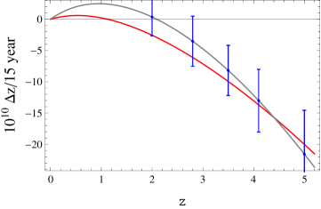
Figure 2: The redshift drift curve for the $\Lambda$CDM model (grey curve) and the Stephani model with $\Omega_{\beta,0}=0.68$ and $w\equiv w_{e}(r=0)=-0.08$ found from the intersection of the confidence intervals for SNIa, redshift drift and BAO (red curve) (see Fig.3). Also shown are the simulated redshift drift data with their error bars from Quartin .

With this simulated data set $\chi^{2}$ takes the form:

$$\chi^{2}_{\rm RD}=\sum^{5}_{i=1}\frac{(\Delta z_{\rm obs}(z_{i})-\Delta z_{\rm theo}(z_{i}))^{2}}{\sigma^{2}_{i}}~{},$$ (IV.11)

where $\Delta z_{\rm obs}(z_{i})$ and $\Delta z_{\rm theo}(z_{i})$ are the “observed” and the predicted value of the drift at redshift $z_{i}$ and $\sigma_{i}$ is the estimated error of the “observed” value of the redshift drift at $z_{i}$, respectively.

In Fig.2 we present confidence intervals (three contours, denoting roughly 68%, 95% and 99% confidence regions) for each observable.

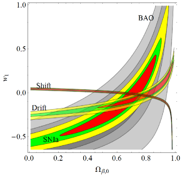
Figure 3: Confidence intervals for the SNIa, redshift drift, BAO and shift parameter. The contours denote roughly 68%, 95% and 99% credible regions. Here a constant equation of state parameter $w\equiv w_{e}(r=0)\equiv w_{1}$ is assumed at the center of symmetry $r=0$. The confidence regions from low redshifts data do not overlap with the confidence region of the shift parameter. An additional problem is that the departure from a standard dust behaviour $w=0$ is significant.

It is evident from Fig. 3 that our Stephani model fits well the data for the SNIa, redshift drift and BAO since the related contours overlap with each other with their 1$\sigma$ CL regions. However the departure of dust from a standard behavior would render this model unviable. In addition, it cannot comply at the same time to the CMB shift constraint. An interesting way of overcoming the latter problem is to replace the constant barotropic index (EoS parameter) $w$ with a function $w(a)$. Because we do not want to change the contours obtained for SNIa, BAO, and the redshift drift, we take $w(a)$ constant on the redshift interval from today up to $z=5$. Further, at some value of the redshift between $z=5$ and the decoupling $z_{dec}$, we assume that the function $w(a)$ suddenly changes its value and then remains constant up to $z_{dec}$.

An example of such function $w(a)$ fulfilling the above requirements is the following (see Fig.4):

$$w(a)=w_{1}+\frac{w_{2}}{2}\left[1+\tanh[\lambda(a_{tr}-a)]\right]~{}.$$ (IV.12)

where $w_{1}$, $w_{2}$, $\lambda$, and $a_{tr}$ are constants.

Figure 4: The time dependent equation of state parameter $w(r=0)=w(a)$ (see eq.(IV.12)) plotted for the particular set of parameters: $\lambda=40$, $a_{tr}=0.08$, $w_{2}=0.4$, $w_{1}=-0.08$ and $\Omega_{\beta,0}=0.68$. Here, the transition occurs for $a\sim 0.08$ which corresponds to the redshift $z\sim 10.49$.

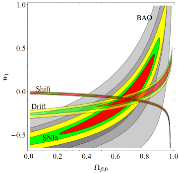
Figure 5: Confidence intervals for the SNIa, redshift drift, BAO and shift parameter for the Stephani model with the scale factor dependent barotropic index $w(r=0)=w(a)$, eq.(IV.12), where the parameters $\lambda=40$, $a_{tr}=0.08$,$w_{2}=0.4$ are fixed. Again the contours denote roughly 68%, 95% and 99% confidence regions.

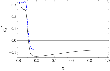
Figure 6: The speeds of sound $c_{S}^{2}(r=0,a)$ (blue dashed curve) and $c_{S}^{2}(r,a)$ (black curve) are shown which corresponds to the barotropic index $w(r=0)=w(a)$, eq.(IV.12) shown on Figure 4. While $c_{S}^{2}(r=0,a)$ differs from $w(a)$ in the region where $w(a)$ changes rapidly, $c_{S}^{2}(r,a)$ includes also the effect of the pressure gradient away from the origin.

As expected, the Stephani model with the barotropic index (IV.12) with $\lambda=40$, $a_{tr}=0.08$ and $w_{1}=-0.08,w_{2}=0.4$ agrees with SNIa and BAO data and the shift parameter, while it recovers essentially the redshift drift in a $\Lambda$CDM model (see Figs.2, 5). Of course, this represents a significant departure from the standard dust behaviour ($w_{1}=0$).

V Results and conclusions

In this paper we have discussed the Stephani models of pressure-gradient spherical shells which are complementary to the varying energy density spherical shells of the Lemaître-Tolman-Bondi models. In our Stephani models there is also a spherical symmetry and in the simplest version considered here we are assumed to be at the center of symmetry $r=0$. A crucial difference between both spherically symmetric inhomogeneous models is the dependence on the radial coordinate $r$ of $g_{00}$ in Stephani models. Comoving observers are no longer following geodesics, and this is basically why a comoving perfect fluid requires a radially dependent pressure in order to counteract the movement in the radial direction. As we have seen, this implies that the real (“effective”) physical pressure depends on both time $t$ or the scale factor $a$ as well as on the radial coordinate $r$. As another general property of these models, we have seen that even if the EoS parameter (barotropic index) $w$ (defined at $r=0$) is constant, the (adiabatic) speed of sound will depend on both $r$ and $a$. In particular, dust ($w=0$) would acquire a negative speed of sound and a negative equation of state parameter $w_{e}$ away from the origin in an accelerating universe. The relative change of the redshift as a function of the (generalized) scale factor $a$ will have a similar behaviour. While we have shown that all these effects remain relatively small, though non negligible at redshifts $z\sim 4$, on our past lightcone in a universe mimicking the cosmic history of our universe, it is nevertheless an interesting physical property.

It is worth emphasizing the difference in the sets of models we have studied and those studied in Ref.chris . Our models presented in Section III and dubbed Models II in Ref.dabrowski95 further specified in Refs.stelmach01 ; GSS are two-component models with one fluid having an arbitrary barotropic equation of state at the center of symmetry and an inhomogeneity playing another fluid with an equation of state of a domain wall type $p=-(2/3)\varrho$. The point is that no explicit form of the scale factor is assumed, but there is a condition $(k/a)^{\centerdot}=0$ which restricts the form of it only slightly. On the other hand, Models I of Ref.dabrowski95 used in Ref.chris in general do not have such a property because for these models $(k/a)^{\centerdot}=-\Delta(\dot{a}/a^{2})$ and this reduces to Models II studied in Ref.dabrowski95 if $\Delta=0$. Besides, these models have the scale factor assumed explicitly at the expense of having a non-barotropic equation of state which only at the center of symmetry reduces to a barotropic one, but with a specific form as for the network of cosmic strings with an equation of state $p=-\frac{1}{3}\varrho$. Because of a general choice of $\Delta$ in Ref.chris , the Models I studied there seem to allow more freedom of the parameters which presumably lead to a larger inhomogeneity secured by generalized EGS theorem chris99 telling us about the admittance of isotropic radiation field to every fundamental observer in the universe.

We have also seen that our best fit model requires the barotropic index $w$ to depend on the generalized scale factor $a$ and to be in the interval $-0.08\lesssim w(a)\lesssim 0.3$, presumably ruling out this model. Indeed, the integrated Sachs-Wolfe effect constraints severely any deviations from the standard dust behavior. We expect that the formation of structure would also be strongly affected.

Another interesting issue concerns compact objects formed through gravitational collapse. While the background perfect fluid is comoving due to its pressure gradient, it is an interesting question whether compact objects that form out of the perfect fluids perturbations will remain essentially comoving and for how long. A detailed study of all these problems including the growth of perturbations can probably not be addressed analytically and is beyond the scope of this work.

Of course, this model can always yield an observationally acceptable universe if all standard components, including some more standard dark energy component are present and additionally if we take a parameter $\beta$ small enough. In that case $\beta$ can be negative as well as positive. This would be the most natural (though minimal) use of such models if observations would point out to some slight inhomogeneity of our universe with a residual spherical symmetry around us. However, as far as we are aware, currently the similar status is given to LTB models - they also require standard dark energy component in the form of $\Lambda-$term and the inhomogeneity should really be small romano .

VI Acknowledgements

A.B., M.P.D., and T.D. were financed by the National Science Center Grant DEC-2012/06/A/ST2/00395.

Appendix A Redshift-drift formula for a general spherically symmetric Stephani model

We remind following Ref. PRD13 that the light emitted by the source at two different times $t_{e}$ and $t_{e}+\delta t_{e}$ will be observed at $t_{o}$ and $t_{o}+\delta t_{o}$ related by

$$\int_{t_{e}}^{t_{o}}\frac{dt}{a(t)}=\int_{t_{e}+\delta t_{e}}^{t_{o}+\delta t_{o}}\frac{dt}{a(t)}~{}.$$ (A.1)

For small $\delta t_{e}$ and $\delta t_{o}$ we have

$$\frac{\delta t_{e}}{a(t_{e})}=\frac{\delta t_{o}}{a(t_{o})}~{}.$$ (A.2)

Bearing in mind (IV.1), the redshift drift has a general definition sandage ; loeb

$$\delta z=\frac{(u_{a}k^{a})(r_{e},t_{e}+\delta t_{e})}{(u_{a}k^{a})(r_{0},t_{0}+\delta t_{0})}-\frac{(u_{a}k^{a})(r_{e},t_{e})}{(u_{a}k^{a})(r_{0},t_{0})}~{},$$ (A.3)

and this can be calculated to first order using the expansions (for higher order expansion see Ref. PLB13 )

$$(u_{a}k^{a})_{o}=(u_{a}k^{a})(r_{0},t_{0})+\frac{\partial\left[(u_{a}k^{a})(r_{0},t_{0})\right]}{\partial t}\delta t_{0},$$ (A.5)

$$(u_{a}k^{a})_{e}=(u_{a}k^{a})(r_{e},t_{e})+\frac{\partial\left[(u_{a}k^{a})(r_{e},t_{e})\right]}{\partial t}\delta t_{e}~{}.$$

¿From (IV.2) we have

$$\frac{\partial}{\partial t}\left(u_{a}k^{a}\right)=-\left(\frac{1}{a}\right)^{\centerdot}-\frac{1}{4}\left(\frac{k}{a}\right)^{\centerdot}r^{2}~{}.$$ (A.6)

Applying (A.5), (A.5), and (A.2) we obtain

$$\frac{\delta z}{\delta t_{0}} = \frac{\left[\left(\frac{1}{a}\right)^{\centerdot}-\frac{1}{4}\left(\frac{k}{a}\right)^{\centerdot}r^{2}\right]_{e}}{\left[1+\frac{1}{4}kr^{2}\right]_{e}}a(t_{e})$$ (A.7)

$$- \frac{\left[\left(\frac{1}{a}\right)^{\centerdot}+\frac{1}{4}\left(\frac{k}{a}\right)^{\centerdot}r^{2}\right]_{o}}{\left[1+\frac{1}{4}kr^{2}\right]_{o}}a(t_{0})(1+z)$$ (A.8)

¿From (A.7) for the Models I given by (II.9) we have

$$\frac{\delta z}{\delta t_{0}}=\frac{a(t_{e})\left(\gamma+\frac{1}{4}\alpha r_{e}^{2}\right)-a(t_{0})(1+z)\left(\gamma+\frac{1}{4}\alpha r_{0}^{2}\right)}{1+\frac{1}{4}\frac{\alpha t_{0}+\sigma}{\gamma t_{0}+\delta}}~{}~{},$$ (A.9)

while for the Models II given by (III.16) we obtain

$$\frac{\delta z}{\delta t_{0}}=-\frac{H_{0}}{1+\frac{1}{4}k(t_{0})r_{0}^{2}}\left[\frac{H_{e}}{H_{0}}-(1+z)\right]~{},$$ (A.10)

where $H_{e}\equiv H(t_{e})=\dot{a}(t_{e})/a(t_{e})$.

References

- (1) V. Sahni, A. A. Starobinsky, Int. J. Mod. Phys. D 9, 373 (2000); T. Padmanabhan, Phys. Rep. 380, 235 (2003); E. J. Copeland, M. Sami and S. Tsujikawa, Int. J. Mod. Phys. D 15, 1753 (2006); V. Sahni, A. A. Starobinsky, Int. J. Mod. Phys. D 15, 2105 (2006); M. Li, X.-D. Li, S. Wang, Y. Wang, Commun. Theor. Phys. 56, 525 (2011); L. Amendola, S. Tsujikawa, Dark Energy: Theory and Observations, Cambridge University Press, 2010.
- (2) J.-P. Uzan, C. Clarkson, and G.F.R. Ellis, Phys. Rev. Lett., 100, 191303 (2008).
- (3) R.R. Caldwell and A. Stebbins Phys. Rev. Lett., 100, 191302 (2008)); C. Clarkson, B. Bassett, and T. H-Ch. Lu, Phys. Rev. Lett., 101, 011301 (2008).
- (4) G. Lemaître, Ann. Soc. Sci. Brux. A53, 51 (1933); R.C. Tolman, Proc. Natl. Acad. Sci. - U.S.A., 20, 169 (1934); H. Bondi, Mon. Not. R. Astr. Soc. 107, 410 (1947).
- (5) H. Stephani, Commun. Math. Phys. 4, 137 (1967); A. Krasiński, Gen. Relativ. Gravit. 15, 673 (1983).
- (6) M.P. Da̧browski, J. Math. Phys. (N.Y.) 34, 1447 (1993).
- (7) M.P. Da̧browski, Astrophys. J. 447, 43 (1995).
- (8) A. Barnes, Gen. Rel. Grav. 4, 105 (1973).
- (9) A. Krasiński, Inhomogeneous Cosmological Models (Cambridge University Press, Cambridge 1997).
- (10) K. Bolejko, A. Krasiński, C. Hellaby, and M.-N. Célérier, Structures in the Universe by Exact Methods - Formation, Evolution, Interactions (Cambridge University Press, Cambridge, England, 2010).
- (11) M.P. Da̧browski and M.A. Hendry, Astrophys. J. 498, 67 (1998).
- (12) M.-N. Célérier, Astron. Astrophys. 362, 840 (2000); K. Tomita, Prog. Theor. Phys. 106, 929 (2001).
- (13) A. Sandage, Astrophys. J. 136, 319 (1962).
- (14) A. Loeb, Astrophys. J. 499, L11 (1998).
- (15) C. Clarkson and R. Maartens, Classical Quantum Gravity 27, 124008 (2010).
- (16) G.F.R. Ellis, S.D. Nel, R. Maartens, W.R. Stoeger, and A.P. Whitman, Phys. Rep. 124, 315 (1985).
- (17) W. Godłowski, J. Stelmach, and M. Szydłowski, Classical Quantum Gravity 21, 3953 (2004).
- (18) R.A. Barrett and C.A. Clarkson, Classical Quantum Gravity 17, 5047 (2000).
- (19) M. Visser, arXiv: 1502.02758.
- (20) C.A. Clarkson and R.A. Barrett, Classical Quantum Gravity 16, 3781 (1999).
- (21) A. Balcerzak and M.P. Da̧browski, Phys. Rev. D87, 063506 (2013).
- (22) A. Balcerzak, M.P. Da̧browski, and T. Denkiewicz, Astrophys. J. 792, 92 (2014).
- (23) R.A. Sussmann, J. Math. Phys. (N.Y.) 28, 1118 (1987); 29, 945 (1988); 29, 1177 (1988).
- (24) J.D. Barrow, Classical Quantum Gravity 21, L79 (2004).
- (25) M.P. Da̧browski, Phys. Rev. D71, 103505 (2005).
- (26) R.A. Vanderveld, E. E. Flanagan, and I. Wasserman, Phys. Rev. D74, 023506 (2006); A. Krasiński, C. Hellaby, K. Bolejko, and M.-N. Célérier, Gen. Relativ. Gravit. 42, 2453 (2010); K. Bolejko, M.-N. Célérier, A. Krasiński, Classical Quantum Gravity 28, 164002 (2011).
- (27) F. Tipler, Phys. Lett. A 64, 8 (1977); A. Królak, Classical Quantum Gravity 3, 267 (1988).
- (28) J.D. Barrow, Class. Quantum Grav. 21, 5619 (2004).
- (29) L. Fernandez-Jambrina and R. Lazkoz, Phys. Rev. D70, 121503(R) (2004).
- (30) M.P. Da̧browski and T. Denkiewicz, AIP Conf. Proc. 1241, 561 (2010).
- (31) R.R. Caldwell, Phys. Lett. B 545, 23 (2002); M.P. Da̧browski, T. Stachowiak and M. Szydłowski, Phys. Rev. D 68, 103519 (2003); R.R. Caldwell, M. Kamionkowski, and N.N. Weinberg, Phys. Rev. Lett. 91, 071301 (2003); P.H. Frampton, Phys. Lett. B 555, 139 (2003).
- (32) L. Fernandez-Jambrina and R. Lazkoz, Phys. Rev. D74, 064030 (2006).
- (33) J. Stelmach and I. Jakacka, Classical Quantum Gravity 18, 2643 (2001).
- (34) M. P. Da̧browski, Ann. Phys. (N.Y.) 248, 199 (1996).
- (35) R.J. Nemiroff, R. Joshi, and B.R. Patla, arXiv: 1402.4522.
- (36) J. Kristian and R.K. Sachs, Astrophys. J. 143, 379 (1966).
- (37) R. Amanullah, et al., Astrophys. J. 716, 712 (2010).
- (38) D. Weinberg, M. Mortonson, D. Eisenstein, C. Hirata, A. Riess, E. Rozo, Phys. Rep.530, 87 (2013).
- (39) A. Balbi and C. Quercellini, Mon. Not. R. Astron. Soc. 382, 1623 (2007).
- (40) J. Liske et al., Monthly Not. R. Astron. Soc. 386, 1192 (2008).
- (41) K. Yagi and N. Seto, Phys. Rev. D83, 044011 (2011).
- (42) C. Quercellini, L. Amendola, A. Balbi, P. Cabella, and M. Quartin, Phys. Rep. 521, 95 (2012).
- (43) C.-M. Yoo, T. Kai, and K.-I. Nakao, Phys. Rev. D83, 043527 (2011).
- (44) D. Wiltshire, Phys. Rev. D80, 123512 (2009).
- (45) P. Mishra, M.-N. Célérier, and T.P. Singh, Phys. Rev. D86, 083520 (2012).
- (46) B. Moraes, D. Polarski, Phys. Rev. D84, 104003 (2011).
- (47) C. Alcock and B. Paczyński, Nature 281, 358 (1979).
- (48) W. Percival et al., Mon. Not. R Astr. Soc. 401, 2148 (2010);
- (49) C. Blake et al., Mon. Not. R Astr. Soc. 415, 2892 (2011); Mon. Not. R Astr. Soc. 418, 1707 (2011).
- (50) F. Beutler et al., Mon. Not. R Astr. Soc. 416, 3017 (2011) .
- (51) L. Anderson et al., arXiv: 1303.4666.
- (52) S. Nesseris and L. Perivolaropoulos, Journ. Cosm. Astrop. Phys. 0701, 018 (2007).
- (53) E. Komatsu et al., Astrophys. J. Suppl. 192, 18 (2011).
- (54) W.J. Percival, B.A. Reid, D.J. Eisenstein, N.A. Bahcall, T. Budavari et al., Mon. Not. Roy. Astron. Soc. 401, 2148 (2010).
- (55) M. Quartin, L. Amendola, Phys. Rev.D81, 043522 (2010).
- (56) J.R. Bond, G. Efstathiou, and M. Tegmark, Mon. Not. Roy. Astron. Soc. 291, L33 (1997).
- (57) D.J. Eisenstein et al., Astroph. J. 633, 560 (2005).
- (58) A. Balcerzak and M.P. Da̧browski, Phys. Lett. B728, 15 (2014).
- (59) A.E. Romano, S. Sanes, M. Sasaki, and A.A. Starobinsky, arXiv: 1311.1476.