Evaluation of Position-related Information in Multipath Components for Indoor Positioning

Abstract

Location awareness is a key factor for a wealth of wireless indoor applications. Its provision requires the careful fusion of diverse information sources. For agents that use radio signals for localization, this information may either come from signal transmissions with respect to fixed anchors, from cooperative transmissions inbetween agents, or from radar-like monostatic transmissions. Using a-priori knowledge of a floor plan of the environment, specular multipath components can be exploited, based on a geometric-stochastic channel model. In this paper, a unified framework is presented for the quantification of this type of position-related information, using the concept of equivalent Fisher information. We derive analytical results for the Cramér-Rao lower bound of multipath-assisted positioning, considering bistatic transmissions between agents and fixed anchors, monostatic transmissions from agents, cooperative measurements inbetween agents, and combinations thereof, including the effect of clock offsets. Awareness of this information enables highly accurate and robust indoor positioning. Computational results show the applicability of the framework for the characterization of the localization capabilities of a given environment, quantifying the influence of different system setups, signal parameters, and the impact of path overlap.

I Introduction

Location awareness is a key component of many future wireless applications. Achieving the needed level of accuracy robustly is still elusive, especially in indoor environments which are characterized by harsh multipath conditions. Promising candidate systems thus either use sensing technologies that provide remedies against multipath or they fuse information from multiple information sources [1, 2]. WLAN-based systems make use of existing infrastructure and exploit the position dependence of the received signal strength [3]. However, the latter shows a relatively large variance w.r.t. the position-related parameters such as the distance, even with an optimized deployment [4].

In Multipath-assisted indoor positioning, multipath components (MPCs) can be associated to the local geometry using a known floor plan. In this way, MPCs can be seen as signals from additional (virtual) anchors (VAs). Ultra-wideband (UWB) signals are used because of their superior time resolution and to facilitate the separation of MPCs. Hence, additional position-related information is exploited that is contained in the radio signals.

This is in contrast to competing approaches, which either detect and avoid non-line-of-sight (NLOS) measurements [5], mitigate errors induced by strong multipath conditions [6], or employ more realistic statistical models for the distribution of the range estimates [7]. Cooperation between agents is another method to increase the amount of available information [8] and thus to reduce the localization outage. Actual exploitation of multipath propagation requires prior knowledge [9]. This can be the floor plan, like in this work and related approaches [10], or a set of known antenna locations to enable beamforming (e.g. in imaging [11]). In an inverse problem, the room geometry can be inferred from the multipath and known measurement locations [12].

Insight on the position-related information that is conveyed in the signals [13] can be gained by an analysis of performance bounds, such as the Cramér-Rao lower bound (CRLB), which is the lower bound of the covariance matrix of an unbiased estimator for a vector parameter. Using the concept of equivalent Fisher information matrices (EFIMs) [14, 15], allows for analytic evaluation of the CRLB by blockwise inversion of the Fisher information matrix (FIM) [16, 17].

A proper channel model is paramount to capture the information contained in MPCs.

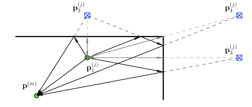
Figure 1: Illustration of multipath geometry using VAs for (i) bistatic transmissions (black) between an anchor at $\mathbf{p}_{\mathrm{1}}^{(j)}$ and an agent at $\mathbf{p}_{\mathrm{}}^{(m)}$ and for (ii) a monostatic measurement (gray) by an agent at $\mathbf{p}_{\mathrm{1}}^{(j)}$.

It is common [18, 19, 20, 21, 22] to differentiate between resolvable MPCs which origin from specular reflections or scatterers and so-called dense or diffuse multipath (DM), which comprises all other “energy producing” components that can not be resolved by the measurement aperture. This part of the channel is often modeled statistically since many unresolvable components add up in one delay bin of the channel impulse response. An established approach to describe these statistics is to use parametric models for the power delay profile (PDP) [18, 19]. The overall models are often referred to as hybrid geometric-stochastic channel models (GSCMs). For the analysis presented in this paper, propagation effects other than the geometrically modeled MPCs constitute interference to useful position-related information. This interference is also called diffuse multipath (DM) [23] and modeled as a colored noise process with non-stationary statistic.

Fig. 1 illustrates the geometric model for multipath-assisted positioning. A signal exchanged between an anchor at position $\mathbf{p}_{\mathrm{1}}^{(j)}$ and an agent at $\mathbf{p}_{\mathrm{}}^{(m)}$ contains specular reflections at the room walls, indicated by the black lines. These reflections can be modeled geometrically using VAs ${\bf p}_{k}^{(j)}$, mirror images of the anchor w.r.t. walls that can be computed from the floor plan [24, 25, 26]. We call this the bistatic setup, where the fixed anchors and the floor plan constitute the available infrastructure. In a cooperative setup, agents localize themselves using bistatic measurements inbetween them. Here, the node at $\mathbf{p}_{\mathrm{1}}^{(j)}$ is an agent that plays the role of an anchor (and thus provides a set of VAs) for the agent at $\mathbf{p}_{\mathrm{}}^{(m)}$. If the agents are equipped accordingly, they can use monostatic measurements, indicated by the gray lines. Here, the node at $\mathbf{p}_{\mathrm{1}}^{(j)}$ acts as anchor for itself with its own set of VAs.

For these measurement setups, we analyze the following scenarios isolated to get insights on different effects of interest: (i) Multipath-Sync with known clock-offset between anchors and agents, (ii) Multipath-NSync with unknown clock-offset between anchors and agents and optionally also between the individual anchors, and (iii) Multipath-Coop with cooperation between the agents, monostatic measurements, and possibly additional fixed anchors. Clock-synchronization for impulse radio UWB has shown to achieve a synchronization accuracy in order of $1\,\text{ns}$, which results still in large localization errors [27]. As a consequence, we estimate the clock-offset jointly, solely based on the received signal and the a-priori known floor plan. Only the differences between the arrival times of MPCs carry position-related information in this case, not the time of arrival as in the synchronized one.

For a tracking application, we have coined the terms multipath-assisted indoor navigation and tracking (MINT) for the bistatic setup [23], and Co-MINT [28] for the cooperative setup. The robustness and accuracy of MINT have been reported in [24, 29, 30] and references therein. Also, a real-time demonstration system has been realized [29].

The key contributions of this paper are:

• We present a mathematical framework for the quantification of position-related information contained in geometrically modeled specular reflections in (ultra) wideband wireless signals under DM.

• This information is quantified for conventional bistatic, monostatic, and cooperative measurement scenarios, optionally including unknown clock offsets, allowing for important insights that can be used in the design of a localization system.

• The results show the relevance of a site-specific, position-related channel model for indoor positioning and the components it comprises of. This position-related FIM is a measure for accuracy and as a further consequence, it can also be seen as indicator for robustness, since it increases with the number of useful MPCs, which also makes algorithms based on multipath-assisted approach more robust.

• We validate, using real measurements, the usefulness of the derived bounds and of the introduced signal-to-interference-plus-noise-ratio (SINR) as a measure for position-related information.

The paper is organized as follows: Section II introduces the geometric-stochastic signal model that is used in Section III to derive the CRLB on the position estimation error. Section IV describes the relationship between signal parameters and node positions in a generic form. These results are used in Section V to derive the CRLB for the different scenarios. Finally, Sections VI and VII wrap up the paper with results, discussions, and conclusions.

Mathematical notations: $\mathbb{E}_{z}\left\{\cdot\right\}$ represents the expectation operator with respect to the random variable $z$. $[{\bf A}]_{n,m}$ is the $(n,m)$-th element of matrix ${\bf A}$; ${\bf A}_{N\times M}$ indicates the size of a matrix. $\|\cdot\|$ is the Euclidean norm, $|\cdot|$ is the absolute value, and $(\ast)$ denotes convolution. ${\bf A}\succeq{\bf B}$ means that ${\bf A}-{\bf B}$ is positive semidefinite. ${\bf I}_{N}$ is the identity matrix of size $N$. $(\cdot{\textbullet})^{\mathrm{H}}$ is the Hermitian conjugate. $\mathrm{tr}\{\cdot\}$ and $\mathrm{diag}\{\cdot\}$ are the trace and the diagonal of a square matrix, respectively.

II Signal Model

In Sections II and III, we simplify the setup—for the ease of readability—to a single (fixed) anchor located at position ${\bf p}_{1}\in\mathbb{R}^{2}$ and one agent at position ${\bf p}\in\mathbb{R}^{2}$. Note that two-dimensional position coordinates are used throughout the paper, for the sake of simplicity. A baseband UWB signal $s(t)$ is exchanged between the anchor and the agent. The corresponding received signal is modeled as [23]

$$r(t) =r_{\det}(t)+r_{\mathrm{diff}}(t)+w(t)$$

$$=\sum_{k=1}^{K}\alpha_{k}s(t-\tau_{k})+(s\ast\nu)(t-\epsilon)+w(t).$$ (1)

The first term $r_{\det}(t)$ describes a sum of $K$ deterministic MPCs with complex amplitudes $\{\alpha_{k}\}$ and delays $\{\tau_{k}\}$. We model these delays by VAs at positions ${\bf p}_{k}\in\mathbb{R}^{2}$, yielding $\tau_{k}=\frac{1}{c}\|{\bf p}-{\bf p}_{k}\|+\epsilon$, with $k=1\ldots K$, where $c$ is the speed of light and $\epsilon$ represents the clock-offset due to clock asynchronism. $K$ is equivalent to the number of visible VAs at the agent position ${\bf p}$ [24]. We assume the energy of $s(t)$ is normalized to one.

The second term $r_{\mathrm{diff}}(t)$ denotes the convolution of the transmitted signal $s(t)$ with the DM $\nu(t)$, which is modeled as a zero-mean Gaussian random process. Note that the statistic of $r_{\mathrm{diff}}(t)$ is non-stationary in the delay domain and it is colored due to the spectrum of $s(t)$. For DM we assume uncorrelated scattering along the delay axis $\tau$, hence the auto-correlation function (ACF) of $\nu(t)$ is given by

$$K_{\nu}(\tau,u)=\mathbb{E}_{\nu}\left\{\nu(\tau)[\nu(u)]^{*}\right\}=S_{\nu}(\tau)\delta(\tau-u),$$ (2)

where $S_{\nu}(\tau)$ is the PDP of DM at the agent position ${\bf p}$. The DM process is assumed to be quasi-stationary in the spatial domain, which means that $S_{\nu}(\tau)$ does not change in the vicinity of position ${\bf p}$ [31]. The PDP $S_{\nu}(\tau)$ is crucial to represent the power ratio between useful deterministic MPCs and DM (along the delay axis $\tau$) and it is represented by an arbitrary function which can be estimated from an ensemble of measurements [19] , rather than a parametric PDP [18]. We will assume that the DM statistic is known a-priori to be able to analyze the influence of DM on the CRLB in closed form, with no parametric restriction on the DM PDP $S_{\nu}(\tau)$. With this, our results will show that information coming from MPCs is quantified by a signal-to-interference-plus-noise-ratio (SINR) for these MPCs, which represents the power ratio between useful deterministic MPC and impairing DM plus noise. Finally, the last term $w(t)$ denotes an additive white Gaussian noise (AWGN) process with double-sided power spectral density (PSD) of $N_{0}/2$.

In the following, we will drop the clock-offset $\epsilon$. We will re-introduce it in Section V-B where the Multipath-NSync setup is studied.

III Cramér-Rao Lower Bound

The goal of multipath-assisted indoor positioning is to estimate the agent’s position ${\bf p}$ from the signal waveform (II), exploiting the knowledge of the VA positions $\{{\bf p}_{k}\}$, in presence of diffuse multipath and AWGN with known statistics. Let $\hat{{\boldsymbol{\theta}}}$ denote the estimate of the position-related parameter vector ${\boldsymbol{\theta}}=[{\bf p}^{\mathrm{T}}\ \Re\boldsymbol{\alpha}^{\mathrm{T}}\ \Im\boldsymbol{\alpha}^{\mathrm{T}}]^{\mathrm{T}}\in\mathbb{R}^{D_{\boldsymbol{\theta}}}$, where $\Re\boldsymbol{\alpha}=[\Re\alpha_{1},\dots,\Re\alpha_{K}]^{\mathrm{T}}$ and $\Im\boldsymbol{\alpha}=[\Im\alpha_{1},\dots,\Im\alpha_{K}]^{\mathrm{T}}$ are the real and imaginary parts of the complex amplitudes $\boldsymbol{\alpha}$, respectively, which are nuisance parameters. According to the information inequality, the error covariance matrix of ${\boldsymbol{\theta}}$ is bounded by [32]

$$\mathbb{E}_{{\bf r}|{\boldsymbol{\theta}}}\left\{\big{(}\hat{{\boldsymbol{\theta}}}-{\boldsymbol{\theta}}\big{)}\big{(}\hat{{\boldsymbol{\theta}}}-{\boldsymbol{\theta}}\big{)}^{\mathrm{H}}\right\}\succeq\boldsymbol{\mathcal{I}}_{\boldsymbol{\theta}}^{-1},$$ (3)

where $\boldsymbol{\mathcal{I}}_{\boldsymbol{\theta}}\in\mathbb{R}^{D_{\boldsymbol{\theta}}\times D_{\boldsymbol{\theta}}}$ is the Fisher information matrix (FIM) and its inverse represents the CRLB of ${\boldsymbol{\theta}}$. We apply the chain rule to derive this CRLB (cf. [14, 17]), i.e., the FIM $\boldsymbol{\mathcal{I}}_{\boldsymbol{\theta}}$ is computed from the FIM of the signal parameter vector ${\boldsymbol{\psi}}=\big{[}\boldsymbol{\tau}^{\mathrm{T}},\Re\boldsymbol{\alpha}^{\mathrm{T}},\Im\boldsymbol{\alpha}^{\mathrm{T}}\big{]}^{\mathrm{T}}\in\mathbb{R}^{D_{\boldsymbol{\psi}}}$, where $\boldsymbol{\tau}=[\tau_{1},\dots,\tau_{K}]^{\mathrm{T}}$ represents the vector of position-related delays. We get

$$\boldsymbol{\mathcal{I}}_{\boldsymbol{\theta}}={\bf J}^{\mathrm{T}}\boldsymbol{\mathcal{I}}_{\boldsymbol{\psi}}{\bf J}$$ (4)

with the Jacobian

$${\bf J} =\frac{\partial{\boldsymbol{\psi}}}{\partial{\boldsymbol{\theta}}}\in\mathbb{R}^{D_{\boldsymbol{\psi}}\times D_{\boldsymbol{\theta}}}.$$ (5)

The FIM $\boldsymbol{\mathcal{I}}_{\boldsymbol{\psi}}\in\mathbb{R}^{D_{\boldsymbol{\psi}}\times D_{\boldsymbol{\psi}}}$ of the signal model parameters can be computed from the likelihood function $f({\bf r}|{\boldsymbol{\psi}})$ of the received signal ${\bf r}$ conditioned on parameter vector ${\boldsymbol{\psi}}$,

$$\boldsymbol{\mathcal{I}}_{\boldsymbol{\psi}} =\mathbb{E}_{{\bf r}|{\boldsymbol{\psi}}}\left\{\left[\frac{\partial}{\partial{\boldsymbol{\psi}}}\ln f({\bf r}|{\boldsymbol{\psi}})\right]\left[\frac{\partial}{\partial{\boldsymbol{\psi}}}\ln f({\bf r}|{\boldsymbol{\psi}})\right]^{\mathrm{T}}\right\}.$$ (6)

III-A Likelihood Function

The likelihood function $f({\bf r}|{\boldsymbol{\psi}})$ is defined for the sampled received signal vector ${\bf r}=[r(0),r({T_{\mathrm{s}}}),\dots,r((N-1){T_{\mathrm{s}}})]^{\mathrm{T}}$ $\in\mathbb{C}^{N}$, containing $N$ samples at rate $1/{T_{\mathrm{s}}}$. Using the assumption that AWGN and DM are both Gaussian, it is given by

$$f({\bf r}|{\boldsymbol{\psi}}) \propto\exp\left\{-({\bf r}-{\bf S}\boldsymbol{\alpha})^{\mathrm{H}}{\bf C}_{\mathrm{n}}^{-1}({\bf r}-{\bf S}\boldsymbol{\alpha})\right\}$$

$$\propto\exp\left\{2\Re\left\{{\bf r}^{\mathrm{H}}{\bf C}_{\mathrm{n}}^{-1}{\bf S}\boldsymbol{\alpha}\right\}-\boldsymbol{\alpha}^{\mathrm{H}}{\bf S}^{\mathrm{H}}{\bf C}_{\mathrm{n}}^{-1}{\bf S}\boldsymbol{\alpha}\right\}$$ (7)

where ${\bf S}=[{\bf s}_{\tau_{1}},\dots,{\bf s}_{\tau_{K}}]\in\mathbb{R}^{N\times K}$ is the signal matrix containing delayed versions ${\bf s}_{\tau_{k}}=[s(-\tau_{k}),s({T_{\mathrm{s}}}-\tau_{k}),\dots,s((N-1){T_{\mathrm{s}}}-\tau_{k})]^{\mathrm{T}}$ of the sampled transmit pulse and ${\bf C}_{\mathrm{n}}=\sigma_{\mathrm{n}}^{2}{\bf I}_{N}+{\bf C}_{\mathrm{c}}\in\mathbb{R}^{N\times N}$ denotes the co-variance matrix of the noise processes. The vector of AWGN samples has variance $\sigma_{\mathrm{n}}^{2}=N_{0}/{T_{\mathrm{s}}}$; the elements of the DM co-variance matrix are given by $[{\bf C}_{\mathrm{c}}]_{n,m}={T_{\mathrm{s}}}\sum_{i=0}^{N-1}S_{\nu}(i{T_{\mathrm{s}}})s(n{T_{\mathrm{s}}}-i{T_{\mathrm{s}}})s(m{T_{\mathrm{s}}}-i{T_{\mathrm{s}}})$ (see Appendix A).

III-B FIM for the Signal Model Parameters

III-B1 General Case

The FIM $\boldsymbol{\mathcal{I}}_{\boldsymbol{\psi}}$ is obtained from (6) with (III-A). Following the notation of [14], it is decomposed according to the subvectors of ${\boldsymbol{\psi}}$ into

$$\boldsymbol{\mathcal{I}}_{\boldsymbol{\psi}}=\left[\begin{array}[]{lll}\boldsymbol{\Lambda}_{\mathrm{A}}&\boldsymbol{\Lambda}_{\mathrm{B}}^{\mathrm{R}}&\boldsymbol{\Lambda}_{\mathrm{B}}^{\mathrm{I}}\\ (\boldsymbol{\Lambda}_{\mathrm{B}}^{\mathrm{R}})^{\mathrm{T}}&\boldsymbol{\Lambda}_{\mathrm{C}}^{\prime}&{\bf 0}\\ (\boldsymbol{\Lambda}_{\mathrm{B}}^{\mathrm{I}})^{\mathrm{T}}&{\bf 0}&\boldsymbol{\Lambda}_{\mathrm{C}}^{\prime}\end{array}\right]=\left[\begin{array}[]{ll}\boldsymbol{\Lambda}_{\mathrm{A}}&\boldsymbol{\Lambda}_{\mathrm{B}}\\ \boldsymbol{\Lambda}_{\mathrm{B}}^{\mathrm{T}}&\boldsymbol{\Lambda}_{\mathrm{C}}\end{array}\right].$$ (8)

Its elements are defined as [32], for example (see also (A.5)),

$$[\boldsymbol{\Lambda}_{\mathrm{B}}^{\mathrm{R}}]_{k,k^{\prime}}=\mathbb{E}_{{\bf r}|{\boldsymbol{\psi}}}\left\{-\frac{\partial^{2}\ln f({\bf r}|{\boldsymbol{\psi}})}{\partial\tau_{k}\partial\Re\alpha_{k^{\prime}}}\right\}$$

which yields with (III-A)

$$[\boldsymbol{\Lambda}_{\mathrm{A}}]_{k,k^{\prime}} =2\Re\left\{\alpha_{k}\alpha^{*}_{k^{\prime}}\left(\frac{\partial{\bf s}_{\tau_{k^{\prime}}}}{\partial\tau_{k^{\prime}}}\right)^{\mathrm{H}}{\bf C}_{\bf n}^{-1}\frac{\partial{\bf s}_{\tau_{k}}}{\partial\tau_{k}}\right\}$$ (9)

$$[\boldsymbol{\Lambda}_{\mathrm{B}}^{\mathrm{R}}]_{k,k^{\prime}} =2\Re\left\{\alpha_{k}\big{(}{\bf s}_{\tau_{k^{\prime}}}\big{)}^{\mathrm{H}}{\bf C}_{\bf n}^{-1}\frac{\partial{\bf s}_{\tau_{k}}}{\partial\tau_{k}}\right\}$$ (10)

$$[\boldsymbol{\Lambda}_{\mathrm{B}}^{\mathrm{I}}]_{k,k^{\prime}} =2\Im\left\{\alpha_{k}\big{(}{\bf s}_{\tau_{k^{\prime}}}\big{)}^{\mathrm{H}}{\bf C}_{\bf n}^{-1}\frac{\partial{\bf s}_{\tau_{k}}}{\partial\tau_{k}}\right\}$$ (11)

$$[\boldsymbol{\Lambda}_{\mathrm{C}}^{\prime}]_{k,k^{\prime}} =2\Re\left\{\big{(}{\bf s}_{\tau_{k}}\big{)}^{\mathrm{H}}{\bf C}_{\bf n}^{-1}{\bf s}_{\tau_{k^{\prime}}}\right\}.$$ (12)

These equations can be used to numerically evaluate the FIM without further assumptions. The CRLB can thus be evaluated, but the inverse of the covariance matrix ${\bf C}_{\mathrm{n}}$, which is needed as a whitening operator [33] to account for the non-stationary DM process, limits the insight it can possibly provide. More insight can be gained under the assumption that the received deterministic MPCs $\{\alpha_{k}s(t-\tau_{k})\}$ are orthogonal, which occurs in practice when MPCs are non-overlapping.

III-B2 Orthogonal MPCs

In this case, the columns of the signal matrix ${\bf S}$ are orthogonal and $\boldsymbol{\Lambda}_{\mathrm{A}}$ becomes diagonal (since ${\bf C}_{\bf n}^{-1}$ is symmetric). Furthermore, $[\boldsymbol{\Lambda}_{\mathrm{B}}]_{k,k^{\prime}}$ is zero (due to the symmetry of the autocorrelation function of $s(t)$) and as a consequence $[\boldsymbol{\Lambda}_{\mathrm{C}}]_{k,k^{\prime}}$ is not needed. The elements of $\boldsymbol{\Lambda}_{\mathrm{A}}$ can then be written as (see Appendix A)

$$[\boldsymbol{\Lambda}_{\mathrm{A}}]_{k,k}=8\pi^{2}\beta^{2}\mathrm{SINR}_{k}\gamma_{k}$$ (13)

where $\beta^{2}=\int_{f}f^{2}|S(f)|^{2}\mathrm{d}f$ is the effective (mean square) bandwidth of the energy-normalized transmit pulse $s(t)\stackrel{{\scriptstyle\mathcal{F}}}{{\longleftrightarrow}}S(f)$,

$$\mathrm{SINR}_{k}:=\frac{\big{|}\alpha_{k}\big{|}^{2}}{N_{0}+{T_{\mathrm{p}}}S_{\nu}(\tau_{k})}$$ (14)

is the signal-to-interference-plus-noise ratio (SINR) of the $k$-th MPC, and $\gamma_{k}$ is the so-called bandwidth extension factor. The product of these three factors quantifies the delay information provided by the $k$-th MPC. It hence provides the following insight for the investigated estimation problem: The interference term ${T_{\mathrm{p}}}S_{\nu}(\tau_{k})$ is determined by the PDP of DM $S_{\nu}(\tau_{k})$ at the delay $\tau_{k}$ of the MPC. It scales with the effective pulse duration ${T_{\mathrm{p}}}$ of the pulse $s(t)$, the reciprocal of its equivalent Nyquist bandwidth $B_{\mathrm{N}}=1/{T_{\mathrm{p}}}$. An increased bandwidth is hence beneficial to suppress DM.

The bandwidth extension quantifies the SINR-gain due to the whitening operation. It is defined as $\gamma_{k}=\beta_{k}^{2}/\beta^{2}$, where $\beta_{k}^{2}$ is the mean square bandwidth of the whitened pulse,

$$\beta_{k}^{2}=\int_{f}f^{2}|\mathrm{S}(f)|^{2}\frac{N_{0}+{T_{\mathrm{p}}}S_{\nu}(\tau_{k})}{N_{0}+|\mathrm{S}(f)|^{2}S_{\nu}(\tau_{k})}\mathrm{d}f.$$ (15)

If the pulse has a block spectrum, we have (due to the energy normalization of $s(t)$) $|S(f)|^{2}={T_{\mathrm{p}}}$ for $|f|\leq B_{\mathrm{N}}/2$, hence $\beta_{k}^{2}=\beta^{2}$ and $\gamma_{k}=1$. I.e., in this case, there is no bandwidth extension due to whitening. The same holds if DM is negligible, i.e. $N_{0}\gg{T_{\mathrm{p}}}S_{\nu}(\tau_{k})$. For the asymptotic case that AWGN is negligible, i.e. $|\mathrm{S}(f)|^{2}S_{\nu}(\tau_{k})\gg N_{0}$, we drop $N_{0}$ in (15) and get a block spectrum that corresponds to the absolute bandwidth of $S(f)$.

In general, $\gamma_{k}$ is a function of the interference-to-noise ratio (INR) ${T_{\mathrm{p}}}S_{\nu}(\tau_{k})/N_{0}$ and can be evaluated numerically. Closed-form results can be given for special cases. E.g. for a root-raised-cosine pulse with roll-off factor $R$, we have $\beta^{2}=B_{\mathrm{N}}^{2}(\frac{1}{12}+\frac{\pi^{2}-8}{4\pi^{2}}R^{2})$ which scales slightly with $R$. In the asymptotic case where DM dominates, we get $\beta_{k}^{2}=\frac{(1+R)^{3}}{12}B_{\mathrm{N}}^{2}$. Hence the bandwidth extension due to the whitening operation can result in an SINR gain of up to about 7 dB at $R=1$. Numerical evaluation shows a $\gamma_{k}$ of 4 dB at $R=0.6$ and INR of 15 dB.

For further analysis, we define the extended SINR

$$\widetilde{\mathrm{SINR}}_{k}=\mathrm{SINR}_{k}\gamma_{k}$$ (16)

which quantifies the delay information provided by MPC $k$ as a function of the signal, interference, and noise levels.

III-C Position Error Bound

The FIM $\boldsymbol{\mathcal{I}}_{\boldsymbol{\psi}}$ of the signal model parameters quantifies the information gained from the measurement ${\bf r}$. The position-related part of this information lies in the MPC delays $\boldsymbol{\tau}$, which are a function of the position $\mathbf{p}_{\mathrm{}}$. To compute the position error bound (PEB), the square-root of the trace of the CRLB on the position error, we need the upper left $2\times 2$ submatrix of the inverse of FIM $\boldsymbol{\mathcal{I}}_{\boldsymbol{\theta}}$,

$$\mathcal{P}\{{\bf p}\}=\sqrt{\mathrm{tr}\left\{\left[\boldsymbol{\mathcal{I}}_{\boldsymbol{\theta}}^{-1}\right]_{2\times 2}\right\}}=\sqrt{\mathrm{tr}\left\{\boldsymbol{\mathcal{I}}_{\bf p}^{-1}\right\}},$$ (17)

which can be obtained with (4) and (5) using the blockwise inversion lemma. This results in the so-called equivalent FIM (EFIM) $\boldsymbol{\mathcal{I}}_{\bf p}$ [14],

$$\boldsymbol{\mathcal{I}}_{\bf p}={\bf H}^{\mathrm{T}}\big{(}\boldsymbol{\Lambda}_{\mathrm{A}}-\boldsymbol{\Lambda}_{\mathrm{B}}\big{(}\boldsymbol{\Lambda}_{\mathrm{C}}\big{)}^{-1}\boldsymbol{\Lambda}_{\mathrm{B}}^{\mathrm{T}}\big{)}{\bf H},$$

which represents the information relevant for the position error bound. Matrix ${\bf H}=\partial\boldsymbol{\tau}/\partial{\bf p}$ is the submatrix of Jacobian (5) that relates to the position-related information, the derivatives of the delay vector $\boldsymbol{\tau}$ w.r.t. postition ${\bf p}$. It describes the variation of the signal parameters w.r.t. the position and can assume different, scenario-dependent forms, depending on the roles of anchors and agents. General expressions for these spatial delay gradients are derived in the next section.

IV Spatial Delay Gradients

The following notations are used to find the elements of matrix ${\bf H}$: ${\bf p}^{(m)}\in\mathbb{R}^{2}$ is the position of the $m$-th agent, where $m\in\mathcal{N}_{m}=\{1,2,\ldots,M\}$. ${\bf p}_{1}^{(j)}\in\mathbb{R}^{2}$ is the position of the $j$-th fixed anchor, $j\in\mathcal{N}_{j}=\{M+1,\ldots,M+J\}$, with VAs at positions ${\bf p}_{k}^{(j)}\in\mathbb{R}^{2}$. In the cooperative scenario, we replace $j$ with an arbitrary index $\xi$ to cover fixed anchors as well as agents which act as anchors. The corresponding VAs are at ${\bf p}_{k}^{(\xi)}\in\mathbb{R}^{2}$. To describe gradients w.r.t. anchor or agent position, we use an index $\eta$, introducing ${\bf p}^{(\eta)}\in\mathbb{R}^{2}$.

The delay of the $k$-th MPC is defined by the distance between the $k$-th VA and the $m$-th agent,

$$\tau_{k}^{(\xi,m)} =\frac{1}{c}\big{\|}{\bf p}^{(m)}-{\bf p}_{k}^{(\xi)}\big{\|}$$ (18)

$$=\frac{1}{c}\sqrt{\big{(}x^{(m)}-x_{k}^{(\xi)}\big{)}^{2}+\big{(}y^{(m)}-y_{k}^{(\xi)}\big{)}^{2}}.$$ (19)

The angle of vector $({\bf p}^{(m)}-{\bf p}_{k}^{(\xi)})$ is written as $\phi_{k}^{(\xi,m)}$. To describe the relation between the signal parameter $\tau_{k}^{(\xi,m)}$ and the geometry, we need to analyze the spatial delay gradient, the derivative of the delay $\tau_{k}^{(\xi,m)}$ w.r.t. position ${\bf p}^{(\eta)}$,

$${\bf h}_{k}^{(\xi,\eta,m)}= {{\frac{\partial\tau_{k}^{(\xi,m)}}{\partial{\bf p}^{(\eta)}}}}={\frac{1}{c}}{{\frac{\partial\big{\|}{\bf p}^{(m)}-{\bf p}_{k}^{(\xi)}\big{\|}}{\partial{\bf p}^{(\eta)}}}}$$

$$\ = {\frac{1}{c}}{{\frac{\partial\big{(}x^{(m)}-x_{k}^{(\xi)}\big{)}}{\partial{\bf p}^{(\eta)}}}}{\frac{x^{(m)}-x_{k}^{(\xi)}}{\big{\|}{\bf p}^{(m)}-{\bf p}_{k}^{(\xi)}\big{\|}}}\$$

$$+{\frac{1}{c}}{{\frac{\partial\big{(}y^{(m)}-y_{k}^{(\xi)}\big{)}}{\partial{\bf p}^{(\eta)}}}}{\frac{y^{(m)}-y_{k}^{(\xi)}}{\big{\|}{\bf p}^{(m)}-{\bf p}_{k}^{(\xi)}\big{\|}}}$$

$$\ = {\frac{1}{c}}\Big{(}\delta_{m,\eta}{\bf I}_{2}-\delta_{\eta,\xi}{{\frac{\partial{\bf p}_{k}^{(\xi)}}{\partial{\bf p}^{(\xi)}}}}\Big{)}^{\mathrm{T}}{\bf e}\Big{(}\phi_{k}^{(\xi,m)}\Big{)}$$ (20)

where ${\bf e}(\phi):=[\cos(\phi),\sin(\phi)]^{\mathrm{T}}$ is a unit vector in direction of the argument angle and $\delta_{m,\eta}$ is the Kronecker delta.Using (B.14) for the Jacobian ${{\bf p}_{k}^{(\xi)}}/{{\bf p}^{(\xi)}}$ of a VA position w.r.t. its respective anchor’s position from Appendix B, we get

$${\bf h}_{k}^{(\xi,\eta,m)}=$$ (21)

$$\qquad{\frac{1}{c}}\Big{[}\delta_{m,\eta}{\bf e}\Big{(}\phi_{k}^{(\xi,m)}\Big{)}\ -\delta_{\eta,\xi}{\bf e}\Big{(}(-1)^{Q_{k}^{(\xi)}}\phi_{k}^{(\xi,m)}+2\bar{\zeta}_{k}^{(\xi)}\Big{)}\Big{]},$$

where the first summand represents the influence of the agent position while the second summand is linked to the anchor position. The parameter $\bar{\zeta}_{k}^{(\xi)}$ (see Appendix B) describes the effective wall angle of the $k$-th MPC w.r.t. to the $\eta$-th anchor (or agent) and $Q_{k}^{(\xi)}$ represents the according VA order. We stack the transposed gradient vectors (21) for the entire set of multipath components in the gradient matrix ${\bf H}^{(\xi,\eta,m)}\in\mathbb{R}^{K^{(\xi,m)}\times 2}$ and the matrices for all the agents’ derivatives into matrix ${\bf H}^{(\xi,m)}\in\mathbb{R}^{K^{(\xi,m)}\times 2M}$.

The following specializations will be used:

IV-1 Bistatic scenario

$k=1,\ldots,K^{(\xi,m)}$

The gradient with respect to the agent

This case describes the derivatives of delay $\tau^{(\xi,m)}$ w.r.t. the agent position, i.e. $\eta=m$, yielding the gradient

$${\bf h}_{k}^{(\xi,m,m)}={{\frac{\partial\tau^{(\xi,m)}}{\partial{\bf p}^{(m)}}}}={\frac{1}{c}}{\bf e}\Big{(}\phi_{k}^{(\xi,m)}\Big{)}$$ (22)

which represents a vector pointing from an agent to the $k$-th VA of the according anchor. We define the gradient matrix ${\bf H}_{\text{Ag}}^{(\xi,m)}={\bf H}^{(\xi,m,m)}\in\mathbb{R}^{K^{(\xi,m)}\times 2}$.

The gradient with respect to the anchor

In this case, the derivatives w.r.t. the anchor position ${\bf p}^{(\xi)}={\bf p}_{1}^{(\xi)}$ are described, i.e. $\eta=\xi$. For the $k$-th MPC, the gradient is expressed as

$${\bf h}_{k}^{(\xi,\xi,m)} ={{\frac{\partial\tau_{k}^{(\xi,m)}}{\partial{\bf p}^{(\xi)}}}}$$ (23)

$$=-{\frac{1}{c}}{\bf e}\Big{(}(-1)^{Q_{k}^{(\xi)}}\phi_{k}^{(\xi,m)}+2\bar{\zeta}_{k}^{(\xi)}\Big{)}={\frac{1}{c}}{\bf e}\Big{(}\phi_{k}^{(m,\xi)}\Big{)}$$

which in this case is a vector pointing from an agent acting as anchor to the $k$-th VA of a cooperating agent. The proof for the final equality can be obtained graphically. The gradient matrix is ${\bf H}_{\text{An}}^{(\xi,m)}={\bf H}_{\text{Ag}}^{(m,\xi)}={\bf H}^{(\xi,\xi,m)}\in\mathbb{R}^{K^{(\xi,m)}\times 2}$.

IV-2 Monostatic scenario

Here we restrict the VA set to $k=2,\ldots,K^{(m,m)}$, the agent is as well the anchor, $\xi=m$, and both move synchronously, $\eta=m$, i.e., the two terms in (21) interact with each other. The gradient

$${\bf h}_{k}^{(m,m,m)}={{\frac{\partial\tau_{k}^{(m,m)}}{\partial{\bf p}^{(m)}}}}$$ (24)

$$={\frac{1}{c}}\left({\bf e}\Big{(}\phi_{k}^{(m,m)}\Big{)}-{\bf e}\Big{(}(-1)^{Q_{k}^{(m)}}\phi_{k}^{(m,m)}+2\bar{\zeta}_{k}^{(m)}\Big{)}\right)$$

$$=\left\{\!\begin{array}[]{ll}{\frac{2}{c}}\sin\!\Big{(}\bar{\zeta}_{k}^{(m)}\Big{)}{\bf e}\Big{(}\phi_{k}^{(m,m)}+\bar{\zeta}_{k}^{(m)}-{\frac{\pi}{2}}\Big{)}&\ \text{If}\ Q_{k}^{(m)}\text{is even}\\ {\frac{2}{c}}\sin\!\Big{(}\bar{\zeta}_{k}^{(m)}-\phi_{k}^{(m,m)}\Big{)}{\bf e}\Big{(}\bar{\zeta}_{k}^{(m)}-{\frac{\pi}{2}}\Big{)}&\ \text{If}\ Q_{k}^{(m)}\text{is odd}\end{array}\right.$$

has been decomposed—as shown in Appendix C—into a magnitude term $0\leq\big{\|}{\bf h}_{k}^{(m,m,m)}\big{\|}\leq{\frac{2}{c}}$ and a resulting direction vector. Both depend on the angle $\phi_{k}^{(m,m)}$, the VA order, and the angles of all contributing walls comprised in $\bar{\zeta}_{k}^{(m)}$. The gradient matrix is ${\bf H}_{\text{Mo}}^{(m)}={\bf H}^{(m,m,m)}\in\mathbb{R}^{(K^{(m,m)}-1)\times 2}$.

The following interpretations apply for the monostatic case: Single reflections ($Q_{k}^{(m)}=1$, $\bar{\zeta}_{k}^{(m)}=\phi_{k}^{(m,m)}\pm{\frac{\pi}{2}}$) and reflections on rectangular corners ($Q_{k}^{(m)}=2$, $\bar{\zeta}_{k}^{(m)}=\pm{\frac{\pi}{2}}$) constitute important types of monostatic VAs. Both have $\partial\tau_{k}^{(m,m)}/\partial{\bf p}^{(m)}={\frac{2}{c}}{\bf e}(\phi_{k}^{(m,m)})$, which is twice as much spatial sensitivity of delays as in the bistatic cases (22) and (23), thus providing higher ranging information. The simplest case of a vanishing gradient (magnitude zero) is a second-order reflection between parallel walls ($Q_{k}^{(m)}=2$, $\bar{\zeta}_{k}^{(m)}=0$).

V CRLB on the Position Error

In this Section, the CRLB on the position error is derived for the three scenarios Multipath-Sync, Multipath-NSync, and a Multipath-Coop scenario.

Using a stack vector ${\boldsymbol{\Psi}}=[{\bf T}^{\mathrm{T}},\Re{{\bf A}}^{\mathrm{T}},\Im{{\bf A}}^{\mathrm{T}}]^{\mathrm{T}}$ of the signal parameters for all relevant nodes, with ${\bf T}$ combining the delays and ${\bf A}$ combining the amplitudes, the Jacobian (5) has the following general structure.

$${\bf J} =\frac{\partial{\boldsymbol{\Psi}}}{\partial{\boldsymbol{\Theta}}}=\left[\begin{array}[]{ccc}{\bf H}&{\bf L}&{\bf 0}\\ {\bf 0}&{\bf 0}&{\bf I}\end{array}\right]$$ (28)

$$=\left[\begin{array}[]{cccc}\partial{\bf T}/\partial{\bf P}&\partial{\bf T}/\partial\boldsymbol{\epsilon}&\partial{\bf T}/\partial\Re{\bf A}&\partial{\bf T}/\partial\Im{\bf A}\\ \partial\Re{\bf A}/\partial{\bf P}&\partial\Re{\bf A}/\partial\boldsymbol{\epsilon}&\partial\Re{\bf A}/\partial\Re{\bf A}&\partial\Re{\bf A}/\partial\Im{\bf A}\\ \partial\Im{\bf A}/\partial{\bf P}&\partial\Im{\bf A}/\partial\boldsymbol{\epsilon}&\partial\Im{\bf A}/\partial\Re{\bf A}&\partial\Im{\bf A}/\partial\Im{\bf A}\end{array}\right]$$ (32)

Vector ${\boldsymbol{\Theta}}=[{\bf P}^{\mathrm{T}},\boldsymbol{\epsilon}^{\mathrm{T}},\Re{{\bf A}}^{\mathrm{T}},\Im{{\bf A}}^{\mathrm{T}}]^{\mathrm{T}}$, spatial delay gradient ${\bf H}=\partial{\bf T}/\partial{\bf P}$, and gradient ${\bf L}=\partial{\bf T}/\partial\boldsymbol{\epsilon}$ are specifically defined for the different cases in the following subsections.

V-A Derivation of the CRLB for Multipath-Sync

Assuming that only one agent is present in Multipath-Sync and Multipath-NSync, we drop the agent index $m$ so that ${\bf P}={\bf p}$, and define $\mathcal{N}_{j}=\{1,2,\ldots,J\}$. We use the geometry for the bistatic scenario, case (a) Section B. The clock-offset $\boldsymbol{\epsilon}$ is considered to be known and zero. Using a suitable signaling scheme, measurements ${\bf r}^{(j)}$ from all $J$ anchors are independent. Hence, the log-likelihood function is defined as

$$\ln f({\bf R}|{\boldsymbol{\Psi}})=\sum_{j\in\mathcal{N}_{j}}\ln f\big{(}{\bf r}^{(j)}|\boldsymbol{\tau}^{(j)},\boldsymbol{\alpha}^{(j)}\big{)},$$ (33)

where ${\bf R}=\big{[}\big{(}{\bf r}^{(1)}\big{)}^{\mathrm{T}},\ldots,\big{(}{\bf r}^{(J)}\big{)}^{\mathrm{T}}\big{]}^{\mathrm{T}}$ combines all measurements and $\boldsymbol{\tau}^{(j)}$ and $\boldsymbol{\alpha}^{(j)}$ are the delay and amplitude vectors respectively, corresponding to measurement ${\bf r}^{(j)}$. The Jacobian ${\bf J}$ has the following structure,

$${\bf J}=\left[\begin{array}[]{ccc}{\bf H}^{(1)}_{K^{(1)}\times 2}&\\ \vdots&\\ {\bf H}^{(J)}_{K^{(J)}\times 2}&\\ &{\bf I}_{D_{\bf I}\times D_{\bf I}}\end{array}\right],$$ (38)

where zero-matrices in the off-diagonal blocks are skipped for clarity and $D_{\bf I}=2\sum_{j=1}^{J}K^{(j)}$. The subblocks ${\bf H}^{(j)}={\bf H}_{\text{Ag}}^{(j,1)}$ account for the geometry as described in Section IV. Due to the independence of the measurements ${\bf r}^{(j)}$, the EFIMs $\boldsymbol{\mathcal{I}}_{\bf p}^{(j)}$ from the $J$ different anchors are additive. Using Equation (4), we can write the EFIM as

$$\boldsymbol{\mathcal{I}}_{\bf p} =$$ (39)

$$\sum_{j\in\mathcal{N}_{j}}\big{(}{\bf H}^{(j)}\big{)}^{\mathrm{T}}\Big{(}\boldsymbol{\Lambda}_{\mathrm{A}}^{(j)}-\boldsymbol{\Lambda}_{\mathrm{B}}^{(j)}\big{(}\boldsymbol{\Lambda}_{\mathrm{C}}^{(j)}\big{)}^{-1}\big{(}\boldsymbol{\Lambda}_{\mathrm{B}}^{(j)}\big{)}^{\mathrm{T}}\Big{)}{\bf H}^{(j)}$$

where $\boldsymbol{\Lambda}_{\mathrm{A}}^{(j)}$, $\boldsymbol{\Lambda}_{\mathrm{B}}^{(j)}$, and $\boldsymbol{\Lambda}_{\mathrm{C}}^{(j)}$ are subblocks of $\boldsymbol{\mathcal{I}}_{\boldsymbol{\psi}}^{(j)}$ defined in (8). Expression (39) simplifies when we assume no path overlap (i.e. orthogonality) between signals from different VAs. In this case, $\boldsymbol{\Lambda}_{\mathrm{B}}={\bf 0}$ and $\boldsymbol{\Lambda}_{\mathrm{A}}$ will be diagonal, as discussed in Section III-B2 and we can then write

$$\boldsymbol{\mathcal{I}}_{\bf p} =\sum_{j\in\mathcal{N}_{j}}\big{(}{\bf H}^{(j)}\big{)}^{\mathrm{T}}\boldsymbol{\Lambda}_{\mathrm{A}}^{(j)}{\bf H}^{(j)}$$

$$\approx\frac{8\pi^{2}\beta^{2}}{c^{2}}\sum_{j\in\mathcal{N}_{j}}\sum_{k=1}^{K^{(j)}}\widetilde{\mathrm{SINR}}_{k}^{(j)}{\bf D}_{\mathrm{r}}(\phi_{k}^{(j)})$$ (40)

where $\widetilde{\mathrm{SINR}}_{k}^{(j)}$ is the extended SINR (eq. 16) for the $j$-th anchor and

$${\bf D}_{\mathrm{r}}(\phi_{k}^{(j)})={\bf e}(\phi_{k}^{(j)}){\bf e}(\phi_{k}^{(j)})^{\mathrm{T}}$$ (41)

is called ranging direction matrix (cf. [14]), a rank-one matrix with an eigenvector in direction of $\phi_{k}^{(j)}$.

Valuable insight is gained from (V-A) and (14). In particular,

• Each VA (i.e. each deterministic MPC) adds some positive term to the EFIM in direction of $\phi_{k}^{(j)}$ and hence reduces the PEB in direction of $\phi_{k}^{(j)}$.

• The $\widetilde{\mathrm{SINR}}_{k}^{(j)}$ determines the magnitude of this contribution as discussed in Section III-B2 (cf. ranging intensity information (RII) in [14]). It is limited by diffuse multipath—an effect that reduces with increased bandwidth—and it can show a significant gain due to the interference whitening if the interference-to-noise ratio is large.

• The effective bandwidth $\beta$ scales the EFIM. Any increase corresponds to a decreased PEB.

Discussion of path overlap (cf. [14]):

• $\tau_{k}-\tau_{k^{\prime}}\ll{T_{\mathrm{p}}}$: In this case the MPCs can not be distinguished and the position-related information is entirely lost.

• $\tau_{k}-\tau_{k^{\prime}}\approx{T_{\mathrm{p}}}$: In this case the MPCs are correlated, but the position-related information can still partly be used. The discrete-time formulation of the CRLB based on (III-A) can quantify this information gain, in contrast to our previous, continuous formulation in [23].

• $\tau_{k}-\tau_{k^{\prime}}\gg{T_{\mathrm{p}}}$: If this holds, the MPCs are considered to be orthogonal and (V-A) can be used if it holds for all $k\neq k^{\prime}$.

V-B Derivation of the CRLB for Multipath-NSync

Next we consider the same setup as before, but assume the clock offsets $\boldsymbol{\epsilon}$ to be unknown parameters. The differences between arrival times still provide position information in this case. When using multiple anchors, we distinguish two different scenarios where either the clocks of all anchors are synchronized among each other, or alternatively no synchronization is present at all. While this does not affect the signal parameter FIM, we need to take it into account when performing the parameter transformation. Apart from the partial derivatives ${\bf L}=\partial{\bf T}/\partial\boldsymbol{\epsilon}$, the terms of the Jacobian are identical for Multipath-Sync and Multipath-NSync, resulting in

$${\bf J}=\left[\begin{array}[]{cccc}{\bf H}_{K^{(1)}\times 2}^{(1)}&{\bf L}^{(1)}_{K^{(1)}\times D_{\boldsymbol{\epsilon}}}&\\ \vdots&\vdots&\\ {\bf H}_{K^{(J)}\times 2}^{(J)}&{\bf L}^{(J)}_{K^{(J)}\times D_{\boldsymbol{\epsilon}}}&\\ &&{\bf I}_{D_{{\bf I}}\times D_{{\bf I}}}\end{array}\right],$$ (46)

where ${\bf L}^{(j)}=\partial\boldsymbol{\tau}^{(j)}/\partial\boldsymbol{\epsilon}$ and $D_{\boldsymbol{\epsilon}}$ is the length of $\boldsymbol{\epsilon}$.

Synchronized anchors: When assuming $\epsilon^{(1)}=\dots=\epsilon^{(J)}=\epsilon$, the vector $\boldsymbol{\epsilon}$ reduces to $\boldsymbol{\epsilon}=\epsilon$. The derivatives of the arrival times with respect to the clock offset are then given by ${\bf L}^{(j)}={\bf l}_{\text{syn}}^{(j)}=[1,\dots,1]^{\mathrm{T}}$. Applying the parameter transformation and computing the block inverse similarly as in (39) leads to additivity of the $3\times 3$ EFIMs $\boldsymbol{\mathcal{I}}_{{\bf p},\epsilon}^{(j)}$ for the extended parameter vector $[{\bf p}^{\mathrm{T}},\epsilon]^{\mathrm{T}}$ (see Appendix D). When neglecting path overlap this expression simplifies to

$$\boldsymbol{\mathcal{I}}_{{\bf p},\epsilon}=\sum_{j\in\mathcal{N}_{j}}\boldsymbol{\mathcal{I}}_{{\bf p},\epsilon}^{(j)}=8\pi^{2}\beta^{2}\sum_{j\in\mathcal{N}_{j}}\sum_{k=1}^{K^{(j)}}\widetilde{\mathrm{SINR}}_{k}^{(j)}{\bf D}_{\mathrm{r},\epsilon}(\phi_{k}^{(j)}),$$ (47)

with

$${\bf D}_{\mathrm{r},\epsilon}(\phi_{k}^{(j)})={\bf v}{\bf v}^{\mathrm{T}},\ {\bf v}=\left[{\frac{1}{c}}\cos(\phi_{k}^{(j)}),\ {\frac{1}{c}}\sin(\phi_{k}^{(j)}),\ 1\right]^{\mathrm{T}}.$$

The inner sum in (47) reveals that the $3\times 3$ EFIMs $\boldsymbol{\mathcal{I}}_{{\bf p},\epsilon}^{(j)}$ are in canonical form. Since ${\bf D}_{r,\epsilon}$ is a positive semidefinite matrix, it highlights that each VA adds information for the estimation of ${\bf p}$ and $\epsilon$, scaled by its extended $\widetilde{\mathrm{SINR}}_{k}$ and $\beta$.

The EFIM $\boldsymbol{\mathcal{I}}_{{\bf p}}$ can be computed from $\boldsymbol{\mathcal{I}}_{{\bf p},\epsilon}$ by again applying the blockwise inversion lemma. When neglecting path overlap, the expression for $\boldsymbol{\mathcal{I}}_{{\bf p}}$ becomes

$$\boldsymbol{\mathcal{I}}_{{\bf p}}=\frac{8\pi^{2}\beta^{2}}{c^{2}}\left[\sum_{j\in\mathcal{N}_{j}}\sum_{k=1}^{K^{(j)}}\widetilde{\mathrm{SINR}}_{k}^{(j)}{\bf D}_{\mathrm{r}}(\phi_{k}^{(j)})-\boldsymbol{\mathcal{C}}\right],$$ (48)

where $\boldsymbol{\mathcal{C}}$ accounts for the (negative) influence of the clock offset estimation with

$$\boldsymbol{\mathcal{C}} =\frac{1}{\sum_{j\in\mathcal{N}_{j}}\sum_{k=1}^{K^{(j)}}\widetilde{\mathrm{SINR}}_{k}^{(j)}}{\bf c}{\bf c}^{\mathrm{T}},$$

$${\bf c} =\sum_{j\in\mathcal{N}_{j}}\sum_{k=1}^{K^{(j)}}\widetilde{\mathrm{SINR}}_{k}^{(j)}{\bf e}(\phi_{k}^{(j)}).$$

Note that Multipath-NSync can theoretically achieve equal performance as Multipath-Sync under the (rather unlikely) condition ${\bf c}={\bf 0}$. Otherwise $\boldsymbol{\mathcal{C}}$ reduces the information, and thereby increases the PEB.

Asynchronous anchors: When having $\epsilon^{(i)}\neq\epsilon^{(j)}$, $\forall i\neq j$, $i,j\in\mathcal{N}_{j}$, we stack all clock offsets in the vector $\boldsymbol{\epsilon}=[\epsilon^{(1)},\dots,\epsilon^{(J)}]^{\mathrm{T}}$. The derivatives of the arrival times with respect to the clock offsets are then given by a gradient matrix ${\bf L}=\partial{\bf T}/\partial\boldsymbol{\epsilon}$ of size $\sum_{j\in\mathcal{N}_{j}}K^{(j)}\times J$ which stacks submatrices ${\bf L}_{\text{asyn}}^{(j)}$ with one nonzero column $[{\bf L}_{\text{asyn}}^{(j)}]_{i,j}=1,\ i=1,\dots,K^{(j)}$. This leads to an additivity of the $2\times 2$ EFIMs as shown in Appendix D, i.e. $\boldsymbol{\mathcal{I}}_{\bf p}=\sum_{j\in\mathcal{N}_{j}}\boldsymbol{\mathcal{I}}_{\bf p}^{(j)}$. When neglecting path overlap, $\boldsymbol{\mathcal{I}}_{\bf p}$ takes the form of (48), but with

$$\boldsymbol{\mathcal{C}}=\sum_{j\in\mathcal{N}_{j}}\frac{1}{\sum_{k=1}^{K^{(j)}}\widetilde{\mathrm{SINR}}_{k}^{(j)}}{\bf c}^{(j)}\big{(}{\bf c}^{(j)}\big{)}^{\mathrm{T}}\ ,$$ (49)

$${\bf c}^{(j)}=\sum_{k=1}^{K^{(j)}}\widetilde{\mathrm{SINR}}_{k}^{(j)}{\bf e}(\phi_{k}^{(j)}).$$

Again, equality with Multipath-Sync is obtained if each ${\bf c}^{(j)}={\bf 0}$, otherwise the PEB is increased.

V-C Derivation of the CRLB for Multipath-Coop

We assume $M$ agents $m\in\mathcal{N}_{m}=\{1,2,\ldots,M\}$ and $J$ fixed anchors $j\in\mathcal{N}_{j}=\{M+1,\ldots,M+J\}$, which cooperate with one another. As outlined in the Introduction, every agent conducts a monostatic measurement, meaning it emits a pulse and receives the multipath signal reflected by the environment, and conventional bistatic measurements with all other agents and the fixed anchors. All measurements are distributed such that every agent is able to exploit information from any of its received and/or transmitted signals. The clock-offsets $\boldsymbol{\epsilon}$ are considered to be zero.

The signal parameter vectors for the $(j,m)$-th received signal ${\bf r}^{(j,m)}$ are defined as $\boldsymbol{\tau}^{(j,m)}=\big{[}\tau_{1}^{(j,m)},\ldots,\tau_{K^{(j,m)}}^{(j,m)}\big{]}^{\mathrm{T}}$ and $\boldsymbol{\alpha}^{(j,m)}=\big{[}\alpha_{1}^{(j,m)},\ldots,\alpha_{K^{(j,m)}}^{(j,m)}\big{]}^{\mathrm{T}}$. For deriving the cooperative EFIM, we stack positions ${\bf p}^{(m)}$ of the $M$ agents into the vector

$${\bf P}=\big{[}\big{(}{\bf p}^{(1)}\big{)}^{\mathrm{T}},\ldots,\big{(}{\bf p}^{(M)}\big{)}^{\mathrm{T}}\big{]}^{\mathrm{T}}\in\mathbb{R}^{2M\times 1}$$ (50)

and all measurements ${\bf r}^{(j,m)}$ in the vector

$${\bf R}=\big{[}\big{(}{\bf r}^{(1,1)}\big{)}^{\mathrm{T}},\ldots,\big{(}{\bf r}^{(1,M)}\big{)}^{\mathrm{T}},\ldots,\big{(}{\bf r}^{(M,M)}\big{)}^{\mathrm{T}},\\ \big{(}{\bf r}^{(M+1,1)}\big{)}^{\mathrm{T}},\ldots,\big{(}{\bf r}^{(M+J,M)}\big{)}^{\mathrm{T}}\big{]}^{\mathrm{T}}\in\mathbb{C}^{D_{\bf R}\times 1},$$ (51)

where $D_{\bf R}=NM(M+J)$. Further, we stack the signal parameters correspondingly in the vectors

$${\bf T}=\big{[}\big{(}\boldsymbol{\tau}^{(1,1)}\big{)}^{\mathrm{T}},\ldots,\big{(}\boldsymbol{\tau}^{(1,M)}\big{)}^{\mathrm{T}},\ldots,\big{(}\boldsymbol{\tau}^{(M+J,M)}\big{)}^{\mathrm{T}}\big{]}^{\mathrm{T}}$$ (52)

and

$${\bf A}=\big{[}\big{(}\boldsymbol{\alpha}^{(1,1)}\big{)}^{\mathrm{T}},\ldots,\big{(}\boldsymbol{\alpha}^{(1,M)}\big{)}^{\mathrm{T}},\ldots,\big{(}\boldsymbol{\alpha}^{(M+J,M)}\big{)}^{\mathrm{T}}\big{]}^{\mathrm{T}}$$ (53)

of length $D_{\bf T}=D_{\bf A}=\sum_{j\in(\mathcal{N}_{m}\cup\mathcal{N}_{j})}\sum_{m\in\mathcal{N}_{m}}K^{(j,m)}$ to construct vector ${\boldsymbol{\Psi}}=[{\bf T}^{\mathrm{T}},\Re{\bf A}^{\mathrm{T}},\Im{\bf A}^{\mathrm{T}}]^{\mathrm{T}}$ . The corresponding joint log-likelihood function, assuming independent measurements ${\bf r}^{(j,m)}$ between the cooperating nodes, is defined as

$$\ln f({\bf R}|{\boldsymbol{\Psi}})=\sum_{j\in(\mathcal{N}_{m}\cup\mathcal{N}_{j})}\sum_{m\in\mathcal{N}_{m}}\ln f\big{(}{\bf r}^{(j,m)}|\boldsymbol{\tau}^{(j,m)},\boldsymbol{\alpha}^{(j,m)}\big{)}.$$ (54)

The EFIM $\boldsymbol{\mathcal{I}}_{\bf P}$ is described by (see Appendix E)

$$\boldsymbol{\mathcal{I}}_{\bf P}=\sum_{j\in(\mathcal{N}_{m}\cup\mathcal{N}_{j})}\sum_{m\in\mathcal{N}_{m}}\big{(}{\bf H}^{(j,m)}\big{)}^{\mathrm{T}}\boldsymbol{\Lambda}^{(j,m)}{\bf H}^{(j,m)}$$ (55)

where

$$\boldsymbol{\Lambda}^{(j,m)}=\boldsymbol{\Lambda}_{\mathrm{A}}^{(j,m)}-\boldsymbol{\Lambda}_{\mathrm{B}}^{(j,m)}\big{(}\boldsymbol{\Lambda}_{\mathrm{C}}^{(j,m)}\big{)}^{-1}\big{(}\boldsymbol{\Lambda}_{\mathrm{B}}^{(j,m)}\big{)}^{\mathrm{T}}$$ (56)

yields the sub-blocks $\boldsymbol{\mathcal{I}}_{\boldsymbol{\psi}}^{(j,m)}$ of the FIM for the likelihood function (54), for independent measurements, and ${\bf H}^{(j,m)}$ are the spatial delay gradients of the Jacobian

$${\bf J}\!=\!\left[\!\begin{array}[]{cccc}{\bf H}_{K^{(1,1)}\times 2M}^{(1,1)}&\\ \vdots&\\ {\bf H}_{K^{(1,M)}\times 2M}^{(1,M)}&\\ \vdots&\\ {\bf H}_{K^{(M+J,M)}\times 2M}^{(M+J,M)}&\\ &{\bf I}_{D_{\bf I}\times D_{\bf I}}\end{array}\!\right],$$ (63)

where $D_{\bf I}=2D_{\bf A}$. As shown in Appendix E, one gets the following final result for the EFIM $\boldsymbol{\mathcal{I}}_{\bf p}$ for all agents

$$\boldsymbol{\mathcal{I}}_{\bf P}=\left[\begin{array}[]{cccr}\boldsymbol{\mathcal{I}}_{\mathrm{Mo}}^{(1)}\!+\!2\boldsymbol{\mathcal{I}}_{\mathrm{Ag}}^{(1)}\!+\!\boldsymbol{\mathcal{I}}_{\mathrm{An}}^{(1)}&2\boldsymbol{\mathcal{I}}_{\mathrm{C}}^{(1,2)}&\ldots&2\boldsymbol{\mathcal{I}}_{\mathrm{C}}^{(1,M)}\\ 2\boldsymbol{\mathcal{I}}_{\mathrm{C}}^{(2,1)}&\lx@intercol\ddots\hfil\lx@intercol&\\ \!\vdots\!&&&\\ 2\boldsymbol{\mathcal{I}}_{\mathrm{C}}^{(M,1)}&\lx@intercol\hfil\boldsymbol{\mathcal{I}}_{\mathrm{Mo}}^{(M)}\!+\!2\boldsymbol{\mathcal{I}}_{\mathrm{Ag}}^{(M)}\!+\!\boldsymbol{\mathcal{I}}_{\mathrm{An}}^{(M)}\lx@intercol\end{array}\right].$$ (68)

The diagonal blocks $\boldsymbol{\mathcal{I}}_{\mathrm{Ag}}^{(\eta)}=\sum_{m\in\mathcal{N}_{m}\backslash\{\eta\}}\big{(}{\bf H}_{\text{Ag}}^{(m,\eta)}\big{)}^{\mathrm{T}}\boldsymbol{\Lambda}^{(m,\eta)}{\bf H}_{\text{Ag}}^{(m,\eta)}$ account for the bistatic measurements between agent $\eta$ and all other agents, $\boldsymbol{\mathcal{I}}_{\mathrm{An}}^{(\eta)}=\sum_{j\in\mathcal{N}_{j}}\big{(}{\bf H}_{\text{Ag}}^{(j,\eta)}\big{)}^{\mathrm{T}}\boldsymbol{\Lambda}^{(j,\eta)}{\bf H}_{\text{Ag}}^{(j,\eta)}$ account for the bistatic measurements between agent $\eta$ and all fixed anchors, and $\boldsymbol{\mathcal{I}}_{\mathrm{Mo}}^{(\eta)}=\big{(}{\bf H}_{\text{Mo}}^{(\eta)}\big{)}^{\mathrm{T}}\boldsymbol{\Lambda}^{(\eta,\eta)}{\bf H}_{\text{Mo}}^{(\eta)}$ account for the monostatic measurement of agent $\eta$. The off-diagonal blocks $\boldsymbol{\mathcal{I}}_{\mathrm{C}}^{(\eta,\eta^{\prime})}=\big{(}{\bf H}_{\text{Ag}}^{(\eta^{\prime},\eta)}\big{)}^{\mathrm{T}}\boldsymbol{\Lambda}^{(\eta^{\prime},\eta)}{\bf H}_{\text{Ag}}^{(\eta,\eta^{\prime})}$ account for the uncertainty about the cooperating agents in their role as anchors (cf. (E.2) and (E-2)). This has a negative effect on the localization performance of the agents. The factors of two in (68), related to the EFIM of measurements inbetween agents, results from the fact that those measurements are performed twice. This simplifies the notations in this section. If such repeated measurements are avoided, the same result would apply but with these factors removed.

Finally, the CRLB on position ${\bf p}^{(\eta)}$ of agent $\eta$ is

$$\mathcal{P}\{{\bf p}^{(\eta)}\}=\sqrt{\mathrm{tr}\left\{\left[\boldsymbol{\mathcal{I}}_{\bf P}^{-1}\right]_{2\times 2}^{(\eta,\eta)}\right\}}.$$ (69)

VI Results

TABLE I: Channel parameters for numerical evaluations.

	Param.	Value for Room		Description
		Valid.	Synth.
2cmDeterministic MPCs		2		max. VA order
		$3\,\text{dB}$		attenuation per
				reflection
2cmSignal parameters	${f_{\mathrm{c}}}$	$8\,\text{GHz}$	$7\,\text{GHz}$	carrier freq.
	${T_{\mathrm{p}}}$	$1\,\text{ns}$, ($0.5\,\text{ns}$,$2\,\text{ns}$)		pulse duration
		RRC		pulse shape
	$R$	$0.6$		roll-off factor
2cmPDP of diffuse multipath	$\Omega_{1}$	$2.67\text{e}^{-6}\,\text{}$	$1.16\text{e}^{-6}\,\text{}$	norm. power
	$\gamma_{1}$	$10\,\text{ns}$	$20\,\text{ns}$	shape param.
	$\gamma_{\text{rise}}$	$3\,\text{ns}$	$5\,\text{ns}$
	$\chi$	$0.98$
$\mathrm{E}_{\mathrm{LOS}}/N_{0}$		$29.5\,\text{dB}$ (at $1\,\text{m}$)		LOS SNR

TABLE II: MPC SINRs for the validation environment, estimated from measured signals and computed from the channel model.

	SINR (measurem.) / SINR (model) [dB]
MPC	${T_{\mathrm{p}}}=\mbox{$0.5\,\text{ns}$}$	${T_{\mathrm{p}}}=\mbox{$1\,\text{ns}$}$	${T_{\mathrm{p}}}=\mbox{$2\,\text{ns}$}$
LOS Anchor 1	23.1 / 25.8	24.7 / 24.7	23.2 / 23.7
lower wall	11.1 / 18.3	5.4 / 15.9	4.1 / 13.7
right window	13.5 / 12.6	7.6 / 10.2	6.9 / 7.7
upper wall	2.2 / 11.7	-0.6 / 9.5	5.2 / 7.1
lower wall – right win.	9.5 / 7.3	7.6 / 4.9	4.9 / 2.4
LOS Anchor 2	25.9 / 26.4	26.0 / 25.3	26.5 / 24.2
right window	11.9 / 12.6	10.5 / 10.8	9.3 / 8.8
upper window	10.1 / 14.0	8.2 / 11.6	5.1 / 9.1
left wall	3.1 / 14.4	4.2 / 11.9	5.5 / 9.4
upper wall – right win.	10.6 / 5.7	11.7 / 3.9	3.5 / 1.8
upper win. – left wall	7.2 / 9.7	4.8 / 7.3	2.1 / 4.8

Computational results are presented in this section for two environments. We first validate the theoretical results using experimental data for a room illustrated in Fig. 2 and then discuss in detail the trade-offs of different measurement scenarios for a synthetic room shown in Fig. 3.

For the transmit signal $s(t)$, we use a root-raised-cosine (RRC) pulse with unit energy and a roll-off factor $R=0.6$, modulated on a carrier at ${f_{\mathrm{c}}}=\mbox{$7\,\text{GHz}$}$ and ${f_{\mathrm{c}}}=\mbox{$8\,\text{GHz}$}$ (see Table VI). The computations are done for pulse durations of ${T_{\mathrm{p}}}=0.5\,\text{ns}$, ${T_{\mathrm{p}}}=1\,\text{ns}$ and ${T_{\mathrm{p}}}=2\,\text{ns}$. In the synthetic environments, we assume for all antennas isotropic radiation patterns in the azimuth plane and gains of $0\,\text{dB}$. The free-space pathloss has been modeled by the Friis equation. To account for the material impact, we assume $3\,\text{dB}$ attenuation per reflection. As in our previous paper [23], the PDP of the DM is considered to be a fixed double-exponential function, as introduced by [22, eq. (9)]. This choice reflects the common assumption of an exponential decay of the DM power and also the fact that the LOS component is not impaired by DM as severely as MPCs arriving later [34]. The model has been fitted in [22] to measurements collected in an industrial environment. We have used $\chi=0.98$ as in [22] to describe the impact of DM on the LOS component and adapted $\gamma_{\text{rise}}$ and $\gamma_{1}$ to reflect the smaller dimensions of our environments. Table VI summarizes the parameters of the channel and signal models.

We would like to emphasize that this parametric model was introduced for simplicity and reproducibility, to analyze the impact of DM on the PEB in various scenarios. In practice, the SINR values can be estimated from channel measurements and used with the results from Section V to compute the PEB for real environments. This approach is used next to validate the theoretical results and the parametric channel model.

VI-A Validation with Measurement Data: Multipath-Sync

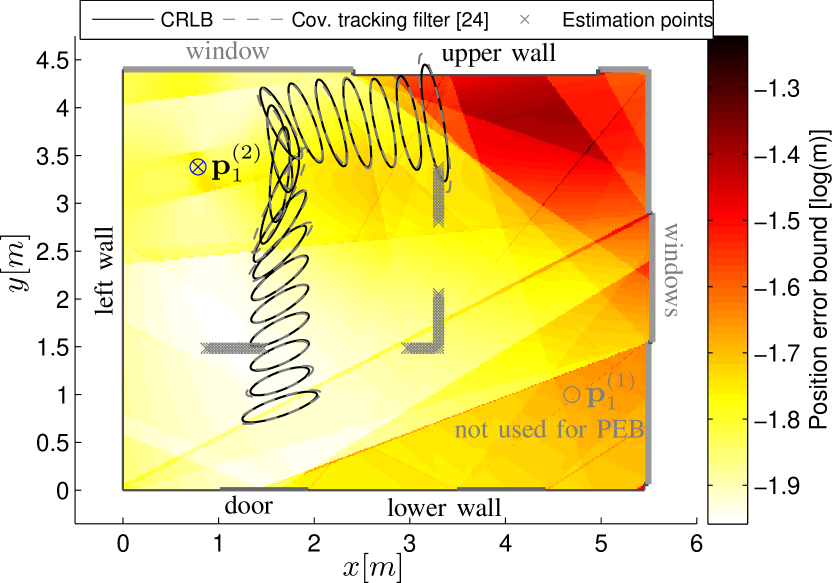
Figure 2: Logarithmic PEB (17) for estimated SINRs in the validation environment using measured signals with ${T_{\mathrm{p}}}=\mbox{$0.5\,\text{ns}$}$ and ${f_{\mathrm{c}}}=\mbox{$8\,\text{GHz}$}$ and only MPCs corresponding to the anchor at $\mathbf{p}_{\mathrm{1}}^{(2)}$. 30-fold standard deviation ellipses are shown for the CRLB and a tracking algorithm (c.f. [24]).

The validation is conducted in an example environment shown in Fig. 2, c.f. [29]. The MPC SINRs (14) are estimated from channel measurement data as discussed in [24, 13], using fixed positions for two anchors and a set of “estimation points” for the agent as illustrated in the figure. Table II shows the obtained values for selected MPCs. It also lists the corresponding SINRs computed from the parametric channel model, with parameters given in Table VI. The choice of the parameters of the double exponential PDP of the DM has been made to account for the smaller room dimensions in comparison to the synthetic environment used below.

The estimated SINRs in Table II show the relevance of the corresponding MPCs. The LOS is the most significant one. Its SINR is approximately constant over all bandwidths used, indicating that it is only slightly influenced by DM. The reflections at the windows and at the lower wall also provide significant position-related information. A scaling with bandwidth—as suggested by (14)—is observable reasonably well. Other MPCs provide less information, such as the left wall (plasterboard) and the upper wall. This is caused by a reduced reflection coefficient, increased interference by DM, and increased variance of the MPC amplitude over the estimation points. Reference [35] contains further results supporting the presented findings based on measurement data from other environments [36].

Table II also shows that the parametric channel model yields realistic SINRs in many cases and therefore valid performance bounds. It has to be stressed that the global PDP model as used here cannot describe the local behavior of DM. However, based on the provided framework, it is straightforward to introduce more realism by fitting separate parameterized or sampled models to any appropriate local area.

Figure 2 shows the logarithmic PEB for the validation environment using the estimated SINRs from Table II for Anchor 2 and ${T_{\mathrm{p}}}=\mbox{$0.5\,\text{ns}$}$. Equation (V-A) has been employed to compute the PEB, i.e. path overlap has been neglected and synchronization assumed. Clearly, one can observe from this figure the visibility regions and the relative importance (c.f. Table II) of specific MPCs. The PEB is better than 10 cm at almost the entire area. The ellipses encode the geometrically decomposed PEB with 30-fold standard deviation, computed from (17). Dashed ellipses are for a multipath-assisted tracking algorithm [24] that makes use of the estimated SINRs for properly weighting the information from MPCs. It can be observed that both results match closely.

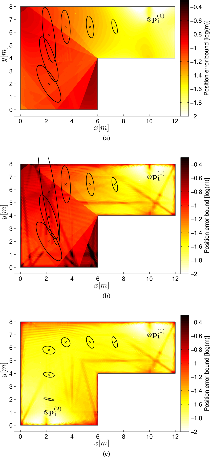
Figure 3: Logarithmic PEB (17) for Multipath-Sync with ${T_{\mathrm{p}}}=1\,\text{ns}$ over the example room for VAs up to order two. (a) One anchor at $\mathbf{p}_{\mathrm{1}}^{(1)}$; path overlap neglected. (b) same as (a) but considering the influence of path overlap. (c) a second anchor has been introduced at $\mathbf{p}_{\mathrm{1}}^{(2)}$; path overlap included. At some sample points, 20-fold standard deviation ellipses are shown.

VI-B Synthetic Environment

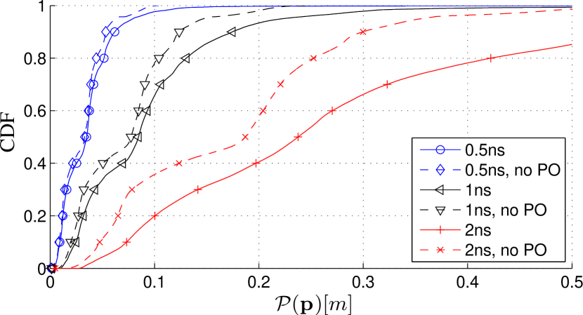
Figure 4: CDFs of the PEB (17) for Multipath-Sync, pulse durations ${T_{\mathrm{p}}}=0.5\,\text{ns}$, ${T_{\mathrm{p}}}=1\,\text{ns}$ and ${T_{\mathrm{p}}}=2\,\text{ns}$, and one anchor at ${\bf p}_{1}^{(1)}$. Path overlap is neglected in results marked by dashed lines.

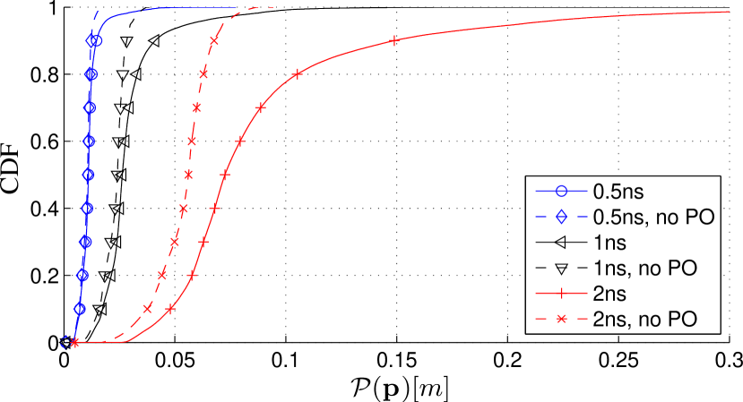
Figure 5: CDFs of the PEB (17) for Multipath-Sync, pulse durations ${T_{\mathrm{p}}}=0.5\,\text{ns}$, ${T_{\mathrm{p}}}=1\,\text{ns}$ and ${T_{\mathrm{p}}}=2\,\text{ns}$, and two anchors at ${\bf p}_{1}^{(1)}$ and ${\bf p}_{1}^{(2)}$. Path overlap is neglected in results marked by dashed lines.

The synthetic environment shown in Fig. 3 is used to compare different measurement scenarios. The PEB is evaluated across the entire room, assuming one or two fixed anchor at positions ${\bf p}_{1}^{(1)}=[10,7]^{\mathrm{T}}$ and ${\bf p}_{1}^{(2)}=[2,1]^{\mathrm{T}}$. We use a point grid with a resolution of $2\,\text{cm}$, resulting in 180,000 points. VAs up to order two are considered, unless otherwise specified.

VI-B1 Multipath-Sync

Fig. 3 shows the PEB over the floor-plan for Multipath-Sync and ${T_{\mathrm{p}}}=1\,\text{ns}$. Figs. 3(a) and (b) compare the simplified PEB neglecting path-overlap (cf. (V-A)) with the full PEB considering it (cf. (39)). A single anchor is employed in both cases at position $\mathbf{p}_{\mathrm{1}}^{(1)}$, yielding a PEB below $10\,\text{cm}$ for most of the area. One can clearly see the visibility regions of different VA-modeled MPCs encoded by the level of the PEB. A valid PEB is obtained over the entire room even though the anchor is partly not visible from the agent positions. If path-overlap is considered (Fig. 3(b)) in the computation of the CRLB, the adverse effect of room symmetries is observable, corresponding to regions where deterministic MPCs overlap. In case of unresolvable path overlap, i.e. the delay difference of two MPCs is less than the pulse duration $\tau_{k}-\tau_{k^{\prime}}\ll{T_{\mathrm{p}}}$, the information of the components is entirely lost (see Section V-A). The ellipses illustrate the geometrically decomposed PEB with 20-fold standard-deviation.

Fig. 3(c) shows the PEB with path-overlap for the same parameters but for two anchors. The error ellipses clearly indicate that the PEB is much smaller and the impact of path overlap has been reduced.

A quantitative assessment of this scenarios is given in Figs. 4 and 5, showing the CDFs of the PEB for different pulse durations (${T_{\mathrm{p}}}=0.5\,\text{ns}$, ${T_{\mathrm{p}}}=1\,\text{ns}$ and ${T_{\mathrm{p}}}=2\,\text{ns}$). One can observe that the PEB increases vastly w.r.t. this parameter. The “no PO” results account for the proportional scaling of Fisher information with bandwidth and additionally for the increased interference power due to DM, both of which are clearly seen in approximation (V-A). The influence of path overlap, which is neglected by (V-A), magnifies this effect even further because its occurrence becomes more probable. It almost diminishes—on the other hand—for the shortest pulse ${T_{\mathrm{p}}}=0.5\,\text{ns}$. Over all, the error magnitude scales by a factor of almost ten, while the bandwidth is scaled by a factor of four.

Our work in [30, 29, 24] shows algorithms based on the presented signal model that can closely approach these bounds. I.e. cm-level accuracy is obtained for $90\,\text{\%}$ of the estimates.

VI-B2 Multipath-NSync

Fig. 6 compares the CDFs of the PEB for Multipath-NSync and different synchronization states inbetween anchors, obtained from (48). The CDFs are shown for either two anchors at ${\bf p}_{1}^{(1)}$ and ${\bf p}_{1}^{(2)}$ which can be synchronized or not, or just the first anchor. A pulse duration of ${T_{\mathrm{p}}}=1\,\text{ns}$ is used. The performance deteriorates w.r.t. the Multipath-Sync case in Figs. 4 and 5, which can be explained by the fact that some of the delay information is used for clock-offset estimation, resulting in a loss of position-related information. A second anchor helps to counteract this effect. Here, one can recognize an additional gain of information if the two anchors are synchronized. The impact of path overlap is smaller if two anchors are used and even less pronounced if the anchors are synchronized.

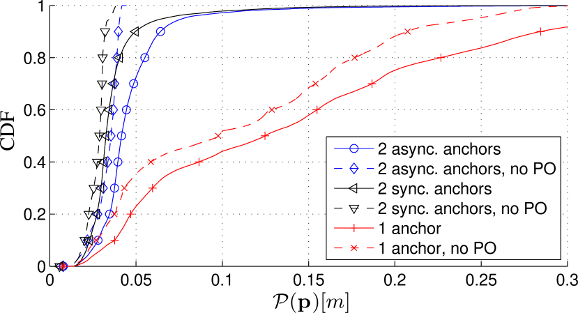
Figure 6: CDFs of the PEB (17) for Multipath-NSync and different synchronization states at pulse duration ${T_{\mathrm{p}}}=1\,\text{ns}$. Either two anchors are used at ${\bf p}_{1}^{(1)}$ and ${\bf p}_{1}^{(2)}$, which can be synchronized or not, or just the first anchor.

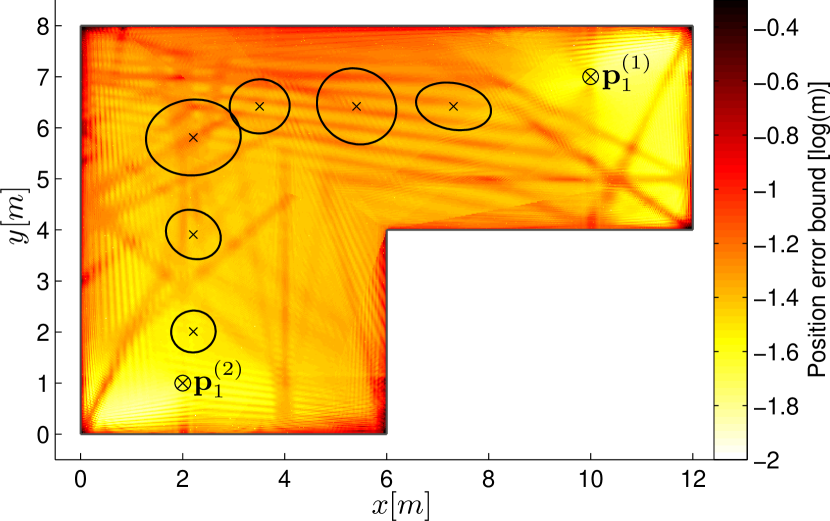
Figure 7: Logarithmic PEB (17) for Multipath-NSync over the example room with ${T_{\mathrm{p}}}=1\,\text{ns}$, using two asynchronous anchors at ${\bf p}_{1}^{(1)}$ and ${\bf p}_{1}^{(2)}$. 20-fold standard deviation ellipses are shown at some sample points.

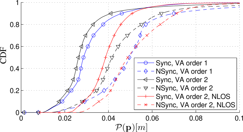
Figure 8: CDFs of the PEB in (17) for Multipath-Sync and Multipath-NSync and ${T_{\mathrm{p}}}=1\,\text{ns}$ with two anchors at ${\bf p}_{1}^{(1)}$ and ${\bf p}_{1}^{(2)}$. VAs of order one or two are considered; for the latter case also for an artificial NLOS situation over the whole room.

A qualitative representation of the PEB is shown in Fig. 7 for Multipath-NSync over the example room, with two anchors at ${\bf p}_{1}^{(1)}$ and ${\bf p}_{1}^{(2)}$, and ${T_{\mathrm{p}}}=1\,\text{ns}$. Comparing this result with the synchronized case shown in Fig. 3(c), one can observe an increase due to the need of extracting syncronization information. Also, the impact of path overlap has increased.

Fig. 8 compares Multipath-Sync and Multipath-NSync for the two-anchors case and ${T_{\mathrm{p}}}=1\,\text{ns}$, considering VAs of order one or two and an NLOS scenario where the LOS component has been set to zero across the entire room. One can observe the importance of the LOS component which usually has a significantly larger SINR and provides thus more position-related information than MPCs arriving later. Increasing the VA order leads in general also to an information gain. However, in a few cases this trend is reversed since a larger VA-order can lead to more positions with unresolvable path overlap. This occurs especially at locations close to walls and in corners.

VI-B3 Multipath-Coop

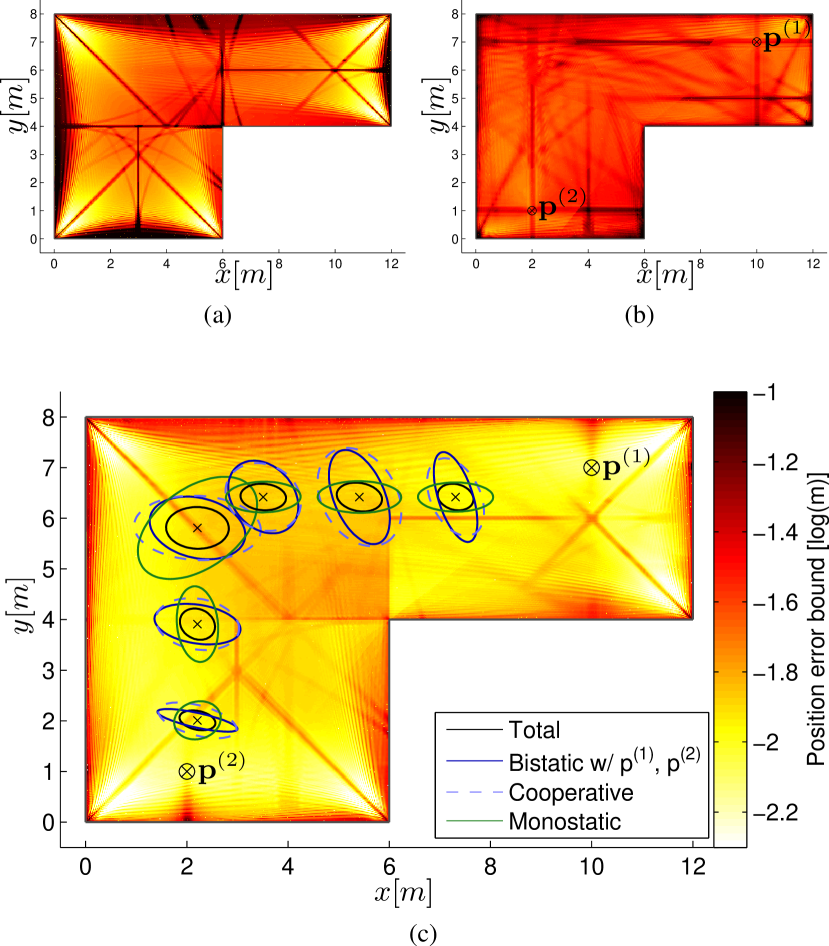
Figure 9: Logarithmic PEB (69) with ${T_{\mathrm{p}}}=1\,\text{ns}$ over the example room for three cooperating agents, two of which are resting at positions ${\bf p}^{(1)}$ and ${\bf p}^{(2)}$. The PEB is decomposed into its (a) monostatic and (b) cooperative components. Plot (c) shows the total PEB for Multipath-Coop. In (c), also the 40-fold standard deviation ellipses are shown at some sample points for these three cases and—in addition—for the (bistatic) case with fixed anchors.

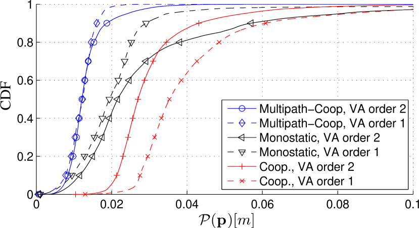
Figure 10: CDFs of the PEB (69) for Multipath-Coop with ${T_{\mathrm{p}}}=1\,\text{ns}$, for VAs of order one and two, analyzing contributions of different measurements.

Fig. 9 contains 2D-plots of the different contributions to the PEB in (69) for the cooperative case. The PEB has been evaluated for Agent 3 across the entire room with two resting, cooperating agents at ${\bf p}^{(1)}$ and ${\bf p}^{(2)}$. In Fig. 9(a), only the monostatic measurements of Agent 3 are considered, illustrating the adverse effect of room symmetries and resulting unresolvable path overlap. In particular, areas close to the walls are affected as well as the diagonals of the room. Fig. 9(b) shows the information provided by the agents at ${\bf p}^{(1)}$ and ${\bf p}^{(2)}$ in their role as anchors. Their contribution is similar to the fixed-anchor case analyzed in Fig. 3(c), but due to uncertainties in their own positions, this information is not fully accessible. A robust, infrastructure-free positioning system is obtained if these two components can complement one another. Indeed Fig. 9(c) indicates excellent performance across the entire area. The distinction between the parts of the position-related information is further highlighted by the CRLB ellipses in Fig. 9(c), which also include the fixed-anchor (bistatic) case of Fig. 3(c). It shows the decreased information of the cooperative part in comparison to the bistatic case with fixed anchors. The monostatic ellipses are mostly oriented towards the nearest wall, where the most significant information comes from. In many cases, this information is nicely complemented by the cooperative contribution.

Fig. 10 shows the CDFs of the PEB in (69) for ${T_{\mathrm{p}}}=\mbox{$1\,\text{ns}$}$ and VAs of order one and two. It is interesting to note that Multipath-Coop does not benefit from taking into account second-order MPCs. This is explained by the large influence of the monostatic measurements, for which second-order reflections cause many regions with unresolvable path overlap (c.f. Fig. 9(a)). For cooperative measurements, increasing the VA order is still beneficial.

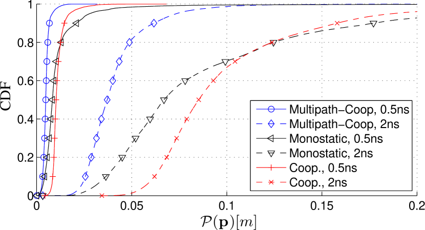
Figure 11: CDFs of the PEB in (69) for Multipath-Coop with ${T_{\mathrm{p}}}=0.5\,\text{ns}$ and ${T_{\mathrm{p}}}=2\,\text{ns}$ for VAs of order two, showing contributions of different measurements types.

Fig. 11 illustrates the influence of bandwidth on Multipath-Coop, using ${T_{\mathrm{p}}}=\mbox{$0.5\,\text{ns}$}$ and ${T_{\mathrm{p}}}=\mbox{$2\,\text{ns}$}$ for VAs of order two. Especially for the monostatic measurements, the occurrence of unresolvable path overlap is significantly reduced, leading to a clear advantage of a larger bandwidth.

VII Conclusions and Outlook

In this article, we have introduced and validated a unified framework for evaluating the accuracy of radio-based indoor-localization methods that exploit geometric information contained in deterministic multipath components. The analysis shows and quantifies fundamental relationships between environment properties and the position-related information that can potentially be acquired. This is due to two mechanisms: (i) Diffuse multipath, which is related to physical properties of the propagation environment, acts as interference to useful specular multipath components. (ii) Path overlap, which relates to system design choices as the placement of agents but also to the given geometry of an environment, may render deterministic components useless. An increased signal bandwidth allows to counteract those effects since it improves the time-resolution of the measurements: The power of DM thus decreases and path overlap becomes less likely.

The framework allows for the analysis of different measurement setups: For instance, (i) in absence of synchronization, position information can be extracted from the time-difference between MPCs. The need for clock-offset estimation reduces thereby the positioning accuracy in comparison to a synchornized setup. (ii) Cooperation between agents increases the available position-related information, but the uncertainty of the unknown positions of agents acting as anchors partly levels this effect. (iii) With monostatic measurements, the VAs move synchronously with the agents, which leads to a scaling of the information provided by MPCs. These MPC-geometry-dependent scaling factors lie between zero and two w.r.t. a conventional bistatic measurement.

The quantification of position-related information, as provided by the presented framework, can be used for designing positioning and tracking algorithms (e.g. [29, 30, 24]). The proper parametrization of the underlying geometric-stochastic channel model optimizes such algorithms and provides valuable insight for system design choices such as antenna placements and signal parameters. Algorithms that can learn and extract these environmental parameters online from measurements may achieve such optimization without the need for manual system optimization and are thus an important topic for further research on robust indoor localization.

Appendix A FIM for orthogonal MPCs

For a sampled received signal, the covariance matrix of AWGN and the DM is written as

$${\bf C}_{\mathrm{n}}=\sigma_{\mathrm{n}}^{2}{\bf I}_{N}+{\bf C}_{\mathrm{c}}=\sigma_{\mathrm{n}}^{2}{\bf I}_{N}+\bar{{\bf S}}^{\mathrm{H}}{\bf S}_{\nu}\bar{{\bf S}}$$ (A.1)

where $\bar{{\bf S}}=[{\bf s}_{0},\cdots,{\bf s}_{N-1}]^{\mathrm{T}}\in\mathbb{R}^{N\times N}$ is the full signal matrix with ${\bf s}_{i}=\Big{[}s((-i)_{\mathrm{mod\,}N}{T_{\mathrm{s}}}),\dots,s((N-1-i)_{\mathrm{mod\,}N}{T_{\mathrm{s}}})\Big{]}^{\mathrm{T}}$, defined as a circulant matrix. The covariance matrix of DM is

$$[\bar{{\bf S}}^{\mathrm{H}}{\bf S}_{\nu}\bar{{\bf S}}]_{n,m}=\sum_{i=0}^{N-1}{T_{\mathrm{s}}}S_{\nu}(i{T_{\mathrm{s}}}) s((n-i)_{\mathrm{mod\,}N}{T_{\mathrm{s}}})$$

$$\times s((m-i)_{\mathrm{mod\,}N}{T_{\mathrm{s}}}).$$ (A.2)

Using the Woodbury matrix identity, the inverse of ${\bf C}_{\mathrm{n}}$ can be written as

$${\bf C}_{\mathrm{n}}^{-1} =\frac{1}{\sigma_{\mathrm{n}}^{2}}\Big{[}{\bf I}_{N}-\bar{{\bf S}}^{\mathrm{H}}\big{(}\sigma_{\mathrm{n}}^{2}{\bf S}_{\nu}^{-1}+\bar{{\bf S}}\bar{{\bf S}}^{\mathrm{H}}\big{)}^{-1}\bar{{\bf S}}\Big{]}.$$ (A.3)

In (III-A), this inverse is multiplied from the right by ${\bf S}\boldsymbol{\alpha}$, which can be re-written as

$${\bf C}_{\mathrm{n}}^{-1}{\bf S}\boldsymbol{\alpha} =\sum_{k=1}^{K}\alpha_{k}{\bf C}_{\mathrm{n}}^{-1}{\bf s}_{\tau_{k}}$$

$$=\frac{1}{\sigma_{\mathrm{n}}^{2}}\sum_{k=1}^{K}\alpha_{k}\Big{[}{\bf I}_{N}-\bar{{\bf S}}^{\mathrm{H}}\big{(}\sigma_{\mathrm{n}}^{2}{\bf S}_{\nu}^{-1}+\bar{{\bf S}}\bar{{\bf S}}^{\mathrm{H}}\big{)}^{-1}\bar{{\bf S}}\Big{]}{\bf s}_{\tau_{k}}$$

where the factor $\bar{{\bf S}}{\bf s}_{\tau_{k}}$ on the very right is an autocorrelation vector of the transmitted signal shifted to delay time $\tau_{k}$. The desired properties of $s(t)$—a large bandwidth and favorable autocorrelation properties—imply that this autocorrelation has most of its energy concentrated at delay $\tau_{k}$. It hence samples the nonstationary PDP at time $\tau_{k}$ and we can replace ${\bf S}_{\nu}$ for each summand by a stationary PDP ${\bf S}_{\nu}^{(\tau_{k})}={T_{\mathrm{s}}}S_{\nu}(\tau_{k}){\bf I}_{N}$. Using this assumption, we define

$$\big{[}{\bf C}_{\mathrm{n}}^{(\tau_{k})}\big{]}^{-1} =\big{[}\sigma_{\mathrm{n}}^{2}{\bf I}_{N}+{T_{\mathrm{s}}}S_{\nu}(\tau_{k})\bar{{\bf S}}^{\mathrm{H}}\bar{{\bf S}}\big{]}^{-1}$$

which involves the inverse of a cyclic matrix that can be diagonalized by a DFT. We introduce a unitary DFT matrix ${\bf W}$, ${\bf W}^{\mathrm{H}}{\bf W}={\bf W}{\bf W}^{\mathrm{H}}={\bf I}$, and use $\bar{{\bf S}}={\bf W}\widetilde{{\bf S}}{\bf W}^{\mathrm{H}}$, where $\widetilde{{\bf S}}=\mathrm{diag}(\sqrt{N}{\bf W}{\bf s}_{0})$ is a diagonal matrix containing the DFT of ${\bf s}_{0}^{\mathrm{T}}$ (the first row of $\bar{{\bf S}}$), to obtain

$$\big{[}{\bf C}_{\mathrm{n}}^{(\tau_{k})}\big{]}^{-1} =\big{[}{\bf W}\big{(}\sigma_{\mathrm{n}}^{2}{\bf I}_{N}+{T_{\mathrm{s}}}S_{\nu}(\tau_{k})\widetilde{{\bf S}}^{\mathrm{H}}\widetilde{{\bf S}}\big{)}{\bf W}^{\mathrm{H}}\big{]}^{-1}$$

$$={\bf W}\big{(}\sigma_{\mathrm{n}}^{2}{\bf I}_{N}+{T_{\mathrm{s}}}S_{\nu}(\tau_{k})\widetilde{{\bf S}}^{\mathrm{H}}\widetilde{{\bf S}}\big{)}^{-1}{\bf W}^{\mathrm{H}}.$$ (A.4)

With this, we can approximate the second summand of likelihood function (III-A) by

$$[\boldsymbol{\alpha}^{\mathrm{H}} {\bf S}^{\mathrm{H}}{\bf C}_{\mathrm{n}}^{-1}{\bf S}\boldsymbol{\alpha}]_{k,k^{\prime}}\approx\alpha_{k}^{*}\alpha_{k^{\prime}}{\bf s}_{\tau_{k}}^{\mathrm{H}}\big{[}{\bf C}_{\mathrm{n}}^{(\tau_{k})}\big{]}^{-1}{\bf s}_{\tau_{k^{\prime}}}$$

$$=\sum_{i=0}^{N-1}\frac{\alpha_{k}^{*}\alpha_{k^{\prime}}|\mathrm{S}_{f}[i]|^{2}}{\sigma_{\mathrm{n}}^{2}+{T_{\mathrm{s}}}|\mathrm{S}_{f}[i]|^{2}S_{\nu}(\tau_{k})}\exp\left\{\frac{-j2\pi i(\tau_{k}-\tau_{k^{\prime}})}{N}\right\}$$

where $\mathrm{S}_{f}[i]$ are samples of the DFT of ${\bf s}_{0}$ and the exponential accounts for the delays $\tau_{k}$ and $\tau_{k^{\prime}}$. Approximating the sum by an integral yields

$$[\boldsymbol{\alpha}^{\mathrm{H}} {\bf S}^{\mathrm{H}}{\bf C}_{\mathrm{n}}^{-1}{\bf S}\boldsymbol{\alpha}]_{k,k^{\prime}}\approx$$

$$\int_{f}\frac{\alpha_{k}^{*}\alpha_{k^{\prime}}|\mathrm{S}(f)|^{2}}{N_{0}+|\mathrm{S}(f)|^{2}S_{\nu}(\tau_{k})}\exp\left\{-j2\pi f(\tau_{k}-\tau_{k^{\prime}})\right\}\mathrm{d}f.$$

With this expression, the diagonal elements of submatrix $\boldsymbol{\Lambda}_{\mathrm{A}}$ of the FIM can be written as

$$[\boldsymbol{\Lambda}_{\mathrm{A}}]_{k,k} =\mathbb{E}_{{\bf r}|{\boldsymbol{\psi}}}\left\{-\frac{\partial^{2}\ln f({\bf r}|{\boldsymbol{\psi}})}{\partial\tau_{k}\partial\tau_{k}}\right\}$$ (A.5)

$$\approx 8\pi^{2}|\alpha_{k}|^{2}\int_{f}f^{2}\frac{|\mathrm{S}(f)|^{2}}{N_{0}+S_{\nu}(\tau_{k})|\mathrm{S}(f)|^{2}}\mathrm{d}f$$

$$=\frac{8\pi^{2}}{N_{0}}\mathrm{SINR}_{k}\int_{f}f^{2}|\mathrm{S}(f)|^{2}\frac{N_{0}+{T_{\mathrm{p}}}S_{\nu}(\tau_{k})}{N_{0}+|\mathrm{S}(f)|^{2}S_{\nu}(\tau_{k})}\mathrm{d}f$$

$$=8\pi^{2}\beta^{2}\mathrm{SINR}_{k}\gamma_{k}$$

where $\beta^{2}=\int_{f}f^{2}|S(f)|^{2}\mathrm{d}f$ is the mean square bandwidth of $s(t)$, $\mathrm{SINR}_{k}=|\alpha_{k}|^{2}/(N_{0}+{T_{\mathrm{p}}}S_{\nu}(\tau_{k}))$ is the signal-to-interference-plus-noise ratio (SINR) of the $k$-th MPC, and $\gamma_{k}=\beta_{k}^{2}/\beta^{2}$ is called bandwidth extension factor, expressing the influence of the whitening. The latter relates the mean square bandwidth of the whitened pulse $\beta_{k}^{2}=\int_{f}f^{2}|\mathrm{S}(f)|^{2}\frac{N_{0}+{T_{\mathrm{p}}}S_{\nu}(\tau_{k})}{N_{0}+|\mathrm{S}(f)|^{2}S_{\nu}(\tau_{k})}\mathrm{d}f$ to $\beta^{2}$. Its value is a function of the interference-to-noise ratio ${T_{\mathrm{p}}}S_{\nu}(\tau_{k})/N_{0}$. Note that $s(t)$ is assumed to be normalized to unit energy. Hence we have $|S(f)|^{2}={T_{\mathrm{p}}}$ for $|f|\leq 1/(2{T_{\mathrm{p}}})$ if $s(t)$ has a block spectrum.

Appendix B Jacobian of VA Position w.r.t. Anchor Position

We want to find a simple expression for $\partial{\bf p}_{k}^{(\xi)}/\partial{\bf p}^{(\xi)}$. We restrict our derivation on a single VA of a specific node w.l.o.g., so we drop all $\xi,k$-indexing and use a simpler notation $\partial{\bf p}_{\text{VA}}/\partial{\bf p}$. As explained in Section I, ${\bf p}_{\text{VA}}$ is obtained by mirroring ${\bf p}$ on walls $Q$ times where $Q$ is the VA order. We use index $q$ for this iteration and refer to the intermediate positions as $\tilde{{\bf p}}_{q}$ where $\tilde{{\bf p}}_{0}={\bf p}$ and $\tilde{{\bf p}}_{Q}={\bf p}_{\text{VA}}$. We need to express ${\bf p}_{\text{VA}}$ as a function of ${\bf p}$ and room geometry. We account for the latter by considering walls with line equations

$$y-y_{q}=\tan(\zeta_{q})(x-x_{q})$$ (B.1)

where $\zeta_{q}$ is the wall angle and ${\bf d}_{q}=(x_{q},y_{q})^{\mathrm{T}}$ is an offset vector. We obtain the $q$-th position by mirroring position $q-1$ on the $q$-th wall, or more formally

$$\tilde{{\bf p}}_{q}=\textbf{Mir}(\tilde{{\bf p}}_{q-1},\zeta_{q},{\bf d}_{q})\ .$$ (B.2)

where Mir is defined as the mirroring operator. Starting at $q=Q$ and using recursive substitution down to $q=0$, we get

$${\bf p}_{\text{VA}}=\textbf{Mir}(\ldots\textbf{Mir}(\textbf{Mir}({\bf p},\zeta_{1},{\bf d}_{1}),\zeta_{2},{\bf d}_{2})\ldots,\zeta_{Q},{\bf d}_{Q})\ .$$ (B.3)

The mirroring operation is given by

$$\textbf{Mir}(\tilde{{\bf p}}_{q-1},\zeta_{q},{\bf d}_{q}) ={\bf M}(\zeta_{q})(\tilde{{\bf p}}_{q-1}-{\bf d}_{q})+{\bf d}_{q}$$ (B.4)

$$={\bf M}(\zeta_{q})\tilde{{\bf p}}_{q-1}+\big{(}{\bf I}-{\bf M}(\zeta_{q})\big{)}{\bf d}_{q}$$

where we use a mirror matrix that acts w.r.t. a line through the origin at angle $\zeta_{q}$,

$${\bf M}(\zeta_{q}) =\left[\begin{array}[]{lr}\cos(2\zeta_{q})&\sin(2\zeta_{q})\\ \sin(2\zeta_{q})&-\cos(2\zeta_{q})\end{array}\right]$$ (B.7)

$$=\textbf{Rot}(2\zeta_{q})\left[\begin{array}[]{rr}1&0\\ 0&-1\end{array}\right]=\textbf{Rot}(2\zeta_{q}){\bf F}$$ (B.10)

and can be decomposed into a rotation by $2\zeta_{q}$, $\textbf{Rot}(2\zeta_{q})$ and a sign-flip ${\bf F}$ in the second dimension. ${\bf M}(\zeta_{q})$ has eigenvalues $\{-1,+1\}$ and bears analogies to rotation. For breaking down (B.3), we prefer the latter form of (B.4) because of the separated $\tilde{{\bf p}}_{q-1}$-summand. By carefully repeated application, we obtain a formula

$${\bf p}_{\text{VA}}={\bf M}(\zeta_{Q})\cdot\tilde{{\bf p}}_{Q-1}+\big{(}{\bf I}-{\bf M}(\zeta_{Q})\big{)}{\bf d}_{Q}$$

$$={\bf M}(\zeta_{Q}){\bf M}(\zeta_{Q-1})\cdot\tilde{{\bf p}}_{Q-2}\ +$$

$$\hskip 13.6572pt{\bf M}(\zeta_{Q})\big{(}{\bf I}-{\bf M}(\zeta_{Q-1})\big{)}{\bf d}_{Q-1}+\big{(}{\bf I}-{\bf M}(\zeta_{Q})\big{)}{\bf d}_{Q}$$

$$=\ \ldots\ =\bigg{(}\prod_{q=0}^{Q-1}{\bf M}(\zeta_{Q-q})\bigg{)}{\bf p}\ +$$

$$\hskip 22.76228pt\sum_{q=1}^{Q}\bigg{(}\prod_{\tilde{q}=1}^{Q-q}{\bf M}(\zeta_{Q+1-\tilde{q}})\bigg{)}\left({\bf I}-{\bf M}(\zeta_{q})\right){\bf d}_{q}$$ (B.11)

where the derivative w.r.t. ${\bf p}$ is just the leading product of mirror matrices. Transposition reverses multiplication order

$$\bigg{(}{\frac{\partial{\bf p}_{\text{VA}}}{\partial{\bf p}}}\bigg{)}^{\mathrm{T}}=\prod_{q=1}^{Q}{\bf M}(\zeta_{q})\ .$$ (B.12)

To resolve this product, we derive a pseudo-homomorphism property of the mirror matrix. We note that both ${\bf F}$ and ${\bf M}(\zeta)$ are symmetric, orthogonal, and self-inverse. Thus, ${\bf M}(\zeta)=\textbf{Rot}(2\zeta){\bf F}$ implies ${\bf M}(\zeta){\bf F}=\textbf{Rot}(2\zeta)$. We rearrange the product of two mirror matrices

$${\bf M}(\zeta_{a}){\bf M}(\zeta_{b}) ={\bf M}(\zeta_{a}){\bf M}(\zeta_{b})^{\mathrm{T}}=\textbf{Rot}(2\zeta_{a}){\bf F}{\bf F}^{\mathrm{T}}\textbf{Rot}(2\zeta_{b})^{\mathrm{T}}$$

$$=\textbf{Rot}(2\zeta_{a}){\bf I}\ \textbf{Rot}(-2\zeta_{b})=\textbf{Rot}(2(\zeta_{a}-\zeta_{b}))$$

and obtain the property

$${\bf M}(\zeta_{a}){\bf M}(\zeta_{b})={\bf M}(\zeta_{a}-\zeta_{b}){\bf F}\ .$$ (B.13)

Applying (B.13) to (B.12) $(Q-1)$-times the Jacobian of a VA position w.r.t. its respective anchor’s position yields

$$\bigg{(}{\frac{\partial{\bf p}_{\text{VA}}}{\partial{\bf p}}}\bigg{)}^{\mathrm{T}}={\bf M}(\bar{\zeta}){\bf F}^{Q-1}=\textbf{Rot}(2\bar{\zeta}){\bf F}^{Q}$$ (B.14)

where we refer to $\bar{\zeta}:=\zeta_{1}-\zeta_{2}+\ldots+(-1)^{Q-1}\zeta_{Q}=\sum_{q=1}^{Q}(-1)^{q-1}\zeta_{q}$ as the effective wall angle, where index $q$ iterates the order of occurrence of walls during MPC reflection or VA construction.

Appendix C Delay Gradient for the Monostatic Setup

We transform the initial gradient from Appendix B into a magnitude-times-unit-vector form by component-wise application of basic trigonometric identities. This yields an insightful expression for the monostatic case, cf. (24). We consider

$${\bf e}(\phi)-{\bf e}((-1)^{Q}\phi+2\bar{\zeta})=\left[\begin{matrix}\cos(\phi)-\cos((-1)^{Q}\phi+2\bar{\zeta})\\ \sin(\phi)-\sin((-1)^{Q}\phi+2\bar{\zeta})\end{matrix}\right]$$

$$=\left[\begin{matrix}2\sin\left({\frac{\left((-1)^{Q}+1\right)\phi+2\bar{\zeta}}{2}}\right)\sin\left(\hphantom{-}{\frac{\left((-1)^{Q}-1\right)\phi+2\bar{\zeta}}{2}}\right)\\ 2\cos\left({\frac{\left((-1)^{Q}+1\right)\phi+2\bar{\zeta}}{2}}\right)\sin\left(-{\frac{\left((-1)^{Q}-1\right)\phi+2\bar{\zeta}}{2}}\right)\end{matrix}\right].$$

By defining symbols for the arguments that contain $\phi$ depending on the even/odd parity of Q

$$O:={\frac{(-1)^{Q}-1}{2}}\phi+\bar{\zeta}=\left\{\begin{array}[]{ll}\bar{\zeta}&\ \text{If}\ Q\ \text{is even}\\ \bar{\zeta}-\phi&\ \text{If}\ Q\ \text{is odd}\end{array}\right.$$

$$E:={\frac{(-1)^{Q}+1}{2}}\phi+\bar{\zeta}=\left\{\begin{array}[]{ll}\bar{\zeta}+\phi&\ \text{If}\ Q\ \text{is even}\\ \bar{\zeta}&\ \text{If}\ Q\ \text{is odd}\end{array}\right.$$

we further get

$${\bf e}(\phi)-{\bf e}((-1)^{Q}\phi+2\bar{\zeta})=2\sin(O)\ {\bf e}\Big{(}E-{\frac{\pi}{2}}\Big{)}$$

$$=\left\{\begin{array}[]{ll}2\sin(\bar{\zeta}){\bf e}(\phi+\bar{\zeta}-{\frac{\pi}{2}})&\ \text{If}\ Q\ \text{is even}\\ 2\sin(\bar{\zeta}-\phi){\bf e}(\bar{\zeta}-{\frac{\pi}{2}})&\ \text{If}\ Q\ \text{is odd}\end{array}\right.\ .$$ (C.3)

Appendix D Derivation of the NSync CRLB

Synchronized anchors: In order to derive the $3\times 3$ EFIM $\boldsymbol{\mathcal{I}}_{{\bf p},\epsilon}$ we need to repartition the transformation matrix ${\bf J}$ by combining the submatrices ${\bf H}^{(j)}$ and ${\bf L}^{(j)}={\bf l}_{\text{syn}}^{(j)}$ to ${\bf G}^{(j)}=[{\bf H}^{(j)},{\bf l}_{\text{syn}}^{(j)}]$. Applying the transformation leads to

$$\boldsymbol{\mathcal{I}}_{\bf P}={\bf J}^{\mathrm{T}}\boldsymbol{\mathcal{I}}_{\boldsymbol{\psi}}{\bf J}=$$ (D.1)

$$\left[\!\begin{array}[]{cccc}\sum\limits_{j\in\mathcal{N}_{j}}\!\big{(}{{\bf G}^{(j)}}\big{)}^{\mathrm{T}}\!\boldsymbol{\Lambda}_{\mathrm{A}}^{(j)}{\bf G}^{(j)}\!&\!\big{(}{{\bf G}^{(1)}}\big{)}^{\mathrm{T}}\!\boldsymbol{\Lambda}_{\mathrm{B}}^{(1)}\!&\!\!\cdots\!\!&\!\big{(}{{\bf G}^{(J)}}\big{)}^{\mathrm{T}}\!\boldsymbol{\Lambda}_{\mathrm{B}}^{(J)}\\ \big{(}{\boldsymbol{\Lambda}_{\mathrm{B}}^{(1)}}\big{)}^{\mathrm{T}}{\bf G}^{(1)}&\boldsymbol{\Lambda}_{\mathrm{C}}^{(1)}\!&\!\!&\!\\ \vdots\!&\!\!&\!\!\ddots\!&\\ \big{(}{\boldsymbol{\Lambda}_{\mathrm{B}}^{(J)}}\big{)}^{\mathrm{T}}{\bf G}^{(J)}\!&\!\!&\!\!&\!\boldsymbol{\Lambda}_{\mathrm{C}}^{(J)}\end{array}\!\right].$$ (D.6)

The $3\times 3$ EFIM is then given as the sum over the EFIMs of the corresponding anchors

$$\boldsymbol{\mathcal{I}}_{{\bf p},\epsilon}=$$ (D.7)

$$\sum_{j\in\mathcal{N}_{j}}\big{(}{{\bf G}^{(j)}}\big{)}^{\mathrm{T}}\Big{[}\boldsymbol{\Lambda}_{\mathrm{A}}^{(j)}-\boldsymbol{\Lambda}_{\mathrm{B}}^{(j)}\big{(}\boldsymbol{\Lambda}_{\mathrm{C}}^{(j)}\big{)}^{-1}\big{(}{\boldsymbol{\Lambda}_{\mathrm{B}}^{(j)}}\big{)}^{\mathrm{T}}\Big{]}{\bf G}^{(j)}.$$

When neglecting path overlap, this reduces to

$$\boldsymbol{\mathcal{I}}_{{\bf p},\epsilon}=\sum_{j\in\mathcal{N}_{j}}\big{(}{{\bf G}^{(j)}}\big{)}^{\mathrm{T}}\boldsymbol{\Lambda}_{\mathrm{A}}^{(j)}{\bf G}^{(j)},$$ (D.8)

which leads finally to (47).

Asynchronous anchors: The result for $\boldsymbol{\mathcal{I}}_{\boldsymbol{\theta}}$ (D.1) is also valid when considering asynchronous anchors, provided that we respect ${\bf L}^{(j)}={\bf L}_{\text{asyn}}^{(j)}$ and ${\bf G}^{(j)}=[{\bf H}^{(j)},{\bf L}_{\text{asyn}}^{(j)}]$. We apply the blockwise inversion lemma twice, first to derive the EFIM $\boldsymbol{\mathcal{I}}_{{\bf p},\boldsymbol{\epsilon}}$ (note that now $\boldsymbol{\epsilon}$ is a vector), and then again to proof the additivity of the EFIMs $\boldsymbol{\mathcal{I}}_{\bf p}^{(j)}$.

The EFIM $\boldsymbol{\mathcal{I}}_{{\bf p},\boldsymbol{\epsilon}}$ is now a square matrix of order $2+J$. It can be expressed as in (D.7), but taking account of the changed definition of ${\bf G}^{(j)}$. We can write its structure as

$$\boldsymbol{\mathcal{I}}_{{\bf p},\boldsymbol{\epsilon}}=\sum_{j\in\mathcal{N}_{j}}\begin{bmatrix}{\boldsymbol{\mathcal{I}}_{A}^{(j)}}&\boldsymbol{\mathcal{I}}_{B}^{(j)}\\ \left(\boldsymbol{\mathcal{I}}_{B}^{(j)}\right)^{\mathrm{T}}&\boldsymbol{\mathcal{I}}_{D}^{(j)}\end{bmatrix},$$ (D.9)

with $\boldsymbol{\mathcal{I}}_{A}^{(j)}\in\mathbb{R}^{2\times 2}$, $\boldsymbol{\mathcal{I}}_{B}^{(j)}\in\mathbb{R}^{2\times J}$ and $\boldsymbol{\mathcal{I}}_{D}^{(j)}\in\mathbb{R}^{J\times J}$. Further evaluation yields, that only the $j$-th column of $\boldsymbol{\mathcal{I}}_{B}^{(j)}$ is nonzero, and the sum over $\boldsymbol{\mathcal{I}}_{B}^{(j)}$ can be written as

$$\sum_{j\in\mathcal{N}_{j}}\boldsymbol{\mathcal{I}}_{B}^{(j)}=\left[{\bf b}^{(1)},\dots,{\bf b}^{(J)}\right],\ {\bf b}^{(j)}\in\mathbb{R}^{2},$$ (D.10)

meaning that each column is determined by the contribution of a different anchors. Similarly, $\boldsymbol{\mathcal{I}}_{D}^{(j)}$ has only one nonzero entry $\left[\boldsymbol{\mathcal{I}}_{D}^{(j)}\right]_{j,j}$, leading to

$$\sum_{j\in\mathcal{N}_{j}}\boldsymbol{\mathcal{I}}_{D}^{(j)}=\text{diag}\left(\left[\boldsymbol{\mathcal{I}}_{D}^{(1)}\right]_{1,1},\dots,\left[\boldsymbol{\mathcal{I}}_{D}^{(J)}\right]_{J,J}\right).$$ (D.11)

Rewriting $\boldsymbol{\mathcal{I}}_{{\bf p},\boldsymbol{\epsilon}}$ (D.9) and again applying the blockwise inversion lemma yields the additivity of the EFIMs $\boldsymbol{\mathcal{I}}_{\bf p}^{(j)}$:

$$\boldsymbol{\mathcal{I}}_{\bf p}=\sum_{j\in\mathcal{N}_{j}}\boldsymbol{\mathcal{I}}_{A}^{(j)}-\frac{1}{\left[\boldsymbol{\mathcal{I}}_{D}^{(j)}\right]_{j,j}}{\bf b}^{(j)}\left({\bf b}^{(j)}\right)^{\mathrm{T}}=\sum_{j\in\mathcal{N}_{j}}\boldsymbol{\mathcal{I}}_{\bf p}^{(j)}.$$ (D.12)

The involved terms are defined by

$$\boldsymbol{\mathcal{I}}_{A}^{(j)}=\big{(}{\bf H}^{(j)}\big{)}^{\mathrm{T}}\Big{(}\boldsymbol{\Lambda}_{\mathrm{A}}^{(j)}-\boldsymbol{\Lambda}_{\mathrm{B}}^{(j)}\big{(}\boldsymbol{\Lambda}_{\mathrm{C}}^{(j)}\big{)}^{-1}\big{(}\boldsymbol{\Lambda}_{\mathrm{B}}^{(j)}\big{)}^{\mathrm{T}}\Big{)}{\bf H}^{(j)},$$

$$\left[\boldsymbol{\mathcal{I}}_{D}^{(j)}\right]_{j,j}=\sum_{u=1}^{K^{(j)}}\sum_{v=1}^{K^{(j)}}\big{[}\boldsymbol{\Lambda}_{\mathrm{A}}^{(j)}-\boldsymbol{\Lambda}_{\mathrm{B}}^{(j)}\big{(}\boldsymbol{\Lambda}_{\mathrm{C}}^{(j)}\big{)}^{-1}\big{(}\boldsymbol{\Lambda}_{\mathrm{B}}^{(j)}\big{)}^{\mathrm{T}}\big{]}_{u,v},$$

and

$${\bf b}^{(j)} =$$

$$\big{(}{\bf H}^{(j)}\big{)}^{\mathrm{T}}\Big{(}\boldsymbol{\Lambda}_{\mathrm{A}}^{(j)}-\boldsymbol{\Lambda}_{\mathrm{B}}^{(j)}\big{(}\boldsymbol{\Lambda}_{\mathrm{C}}^{(j)}\big{)}^{-1}\big{(}\boldsymbol{\Lambda}_{\mathrm{B}}^{(j)}\big{)}^{\mathrm{T}}\Big{)}[1\dots 1]_{1\times K^{(J)}}^{\mathrm{T}}.$$

Appendix E Derivation of the Multipath-Coop CRLB

The EFIM for the cooperative setup is defined as

$$\boldsymbol{\mathcal{I}}_{\bf P}={\bf H}^{\mathrm{T}}\text{diag}\Big{(}\boldsymbol{\Lambda}^{(1,1)},\ldots,\boldsymbol{\Lambda}^{(1,M)},\ldots,\boldsymbol{\Lambda}^{(M+J,M)}\Big{)}{\bf H},$$

being of size $2M\times 2M$. It can be written with subblock ${\bf H}$ from (63) in the canonical form (55). Matrix $\boldsymbol{\Lambda}^{(j,m)}$ is defined in (56). The canonical form decomposes the EFIM $\boldsymbol{\mathcal{I}}_{\bf P}$ into contributions from independent transmissions inbetween the agents or between agents and fixed anchors. Matrix $\boldsymbol{\mathcal{I}}_{\bf P}$ consists of the following subblocks for $\eta,\eta^{\prime}\in\mathcal{N}_{m}=\{1,\ldots,M\}$,

$$\left[\boldsymbol{\mathcal{I}}_{\bf P}\right]_{2\times 2}^{\eta,\eta^{\prime}}\\ =\sum_{j\in(\mathcal{N}_{m}\cup\mathcal{N}_{j})}\sum_{m\in\mathcal{N}_{m}}\big{(}{\bf H}^{(j,\eta,m)}\big{)}^{\mathrm{T}}\boldsymbol{\Lambda}^{(j,m)}{\bf H}^{(j,\eta^{\prime},m)}$$ (E.1)

where ${\bf H}^{(j,\eta,m)}$ stacks the spatial delay gradients (21) as defined in Section IV. Considering that only summand $(j,m)$ of (E.1) contributes to a block, for which either index $j$ or index $m$ equals $\eta$ or $\eta^{\prime}$, we get the following subblocks:

E-1 Off-diagonal blocks $\eta\neq\eta^{\prime}$

$$\left[\boldsymbol{\mathcal{I}}_{\bf P}\right]_{2\times 2}^{(\eta,\eta^{\prime})} =\big{(}{\bf H}^{(j,\eta,m)}\big{)}^{\mathrm{T}}\boldsymbol{\Lambda}^{(j,m)}{\bf H}^{(j,\eta^{\prime},m)}\Big{|}_{j=\eta,m=\eta^{\prime}}$$

$$\quad+\big{(}{\bf H}^{(j,\eta,m)}\big{)}^{\mathrm{T}}\boldsymbol{\Lambda}^{(j,m)}{\bf H}^{(j,\eta^{\prime},m)}\Big{|}_{j=\eta^{\prime},m=\eta}$$

$$=\big{(}{\bf H}_{\text{An}}^{(\eta,\eta^{\prime})}\big{)}^{\mathrm{T}}\boldsymbol{\Lambda}^{(\eta,\eta^{\prime})}{\bf H}_{\text{Ag}}^{(\eta^{\prime},\eta)}$$

$$\quad+\big{(}{\bf H}_{\text{Ag}}^{(\eta^{\prime},\eta)}\big{)}^{\mathrm{T}}\boldsymbol{\Lambda}^{(\eta^{\prime},\eta)}{\bf H}_{\text{An}}^{(\eta^{\prime},\eta)},$$

using the definitions for ${\bf H}_{\text{An}}^{(\eta,\eta^{\prime})}$ and ${\bf H}_{\text{Ag}}^{(\eta,\eta^{\prime})}$ from Section IV-1. With ${\bf H}_{\text{An}}^{(\eta,\eta^{\prime})}={\bf H}_{\text{Ag}}^{(\eta^{\prime},\eta)}$ (Section IV-1) and $\boldsymbol{\Lambda}^{(\eta,\eta^{\prime})}=\boldsymbol{\Lambda}^{(\eta^{\prime},\eta)}$ we get

$$\left[\boldsymbol{\mathcal{I}}_{\bf P}\right]_{2\times 2}^{(\eta,\eta^{\prime})}=2\boldsymbol{\mathcal{I}}_{\mathrm{C}}^{(\eta,\eta^{\prime})}=2\big{(}{\bf H}_{\text{Ag}}^{(\eta^{\prime},\eta)}\big{)}^{\mathrm{T}}\boldsymbol{\Lambda}^{(\eta^{\prime},\eta)}{\bf H}_{\text{Ag}}^{(\eta,\eta^{\prime})}.$$ (E.2)

E-2 Diagonal blocks $\eta=\eta^{\prime}$

$$\left[\boldsymbol{\mathcal{I}}_{\bf P}\right]_{2\times 2}^{\eta,\eta} =\big{(}{\bf H}^{(\eta,\eta,\eta)}\big{)}^{\mathrm{T}}\boldsymbol{\Lambda}^{(\eta,\eta)}{\bf H}^{(\eta,\eta,\eta)}$$

$$\quad+\sum_{\begin{subarray}{c}j\in\mathcal{N}_{m}\backslash\{\eta\}\\ m=\eta\end{subarray}}\big{(}{\bf H}^{(j,\eta,m)}\big{)}^{\mathrm{T}}\boldsymbol{\Lambda}^{(j,m)}{\bf H}^{(j,\eta,m)}$$

$$\quad+\sum_{\begin{subarray}{c}m\in\mathcal{N}_{m}\backslash\{\eta\}\\ j=\eta\end{subarray}}\big{(}{\bf H}^{(j,\eta,m)}\big{)}^{\mathrm{T}}\boldsymbol{\Lambda}^{(j,m)}{\bf H}^{(j,\eta,m)}$$

$$\quad+\sum_{j\in\mathcal{N}_{j}}\left({\bf H}^{(j,\eta,\eta)}\right)^{\mathrm{T}}\boldsymbol{\Lambda}^{(j,\eta)}{\bf H}^{(j,\eta,\eta)}$$

$$=\big{(}{\bf H}_{\text{Mo}}^{(\eta)}\big{)}^{\mathrm{T}}\boldsymbol{\Lambda}^{(\eta,\eta)}{\bf H}_{\text{Mo}}^{(\eta)}$$

$$\quad+\sum_{j\in\mathcal{N}_{m}\backslash\{\eta\}}\big{(}{\bf H}_{\text{Ag}}^{(j,\eta)}\big{)}^{\mathrm{T}}\boldsymbol{\Lambda}^{(j,\eta)}{\bf H}_{\text{Ag}}^{(j,\eta)}$$

$$\quad+\sum_{m\in\mathcal{N}_{m}\backslash\{\eta\}}\big{(}{\bf H}_{\text{An}}^{(\eta,m)}\big{)}^{\mathrm{T}}\boldsymbol{\Lambda}^{(\eta,m)}{\bf H}_{\text{An}}^{(\eta,m)}$$

$$\quad+\sum_{j\in\mathcal{N}_{j}}\big{(}{\bf H}_{\text{Ag}}^{(j,\eta)}\big{)}^{\mathrm{T}}\boldsymbol{\Lambda}^{(j,\eta)}{\bf H}_{\text{Ag}}^{(j,\eta)}$$

using again ${\bf H}_{\text{An}}^{(\eta,\eta^{\prime})}$ and ${\bf H}_{\text{Ag}}^{(\eta,\eta^{\prime})}$ from Section IV-1 and ${\bf H}_{\text{Mo}}^{(\eta)}$ from Section IV-2. With ${\bf H}_{\text{An}}^{(\eta,m)}={\bf H}_{\text{Ag}}^{(m,\eta)}$ and $\boldsymbol{\Lambda}^{(j,m)}=\boldsymbol{\Lambda}^{(m,j)}$ due to reciprocity, we get

$$\left[\boldsymbol{\mathcal{I}}_{\bf P}\right]_{2\times 2}^{(\eta,\eta)} =\boldsymbol{\mathcal{I}}_{\mathrm{Mo}}^{(\eta)}+2\sum_{m\in\mathcal{N}_{m}\backslash\{\eta\}}\boldsymbol{\mathcal{I}}_{\mathrm{Ag}}^{(m,\eta)}+\sum_{j\in\mathcal{N}_{j}}\boldsymbol{\mathcal{I}}_{\mathrm{An}}^{(j,\eta)}$$

$$=\boldsymbol{\mathcal{I}}_{\mathrm{Mo}}^{(\eta)}+2\boldsymbol{\mathcal{I}}_{\mathrm{Ag}}^{(\eta)}+\boldsymbol{\mathcal{I}}_{\mathrm{An}}^{(\eta)}$$ (E.3)

which implicitly defines the contributions from monostatic measurements, bistatic measurements inbetween agents, and bistatic measurements between agents and fixed anchors.

Erik Leitinger (S’12) was born in Graz, Austria, on March 27, 1985. He received the B.Sc. degree (with distinction) in electrical engineering from Graz University of Technology, Graz, Austria, in 2009, and the Dipl.-Ing. degree (with distinction) in electrical engineering from Graz University of Technology, Graz, Austria, in 2012. He is currently pursuing his PhD degree at the Signal Processing and Speech Communication Laboratory (SPSC) of Graz University of Technology, Graz, Austria focused on UWB wireless communication, indoor-positioning, estimation theory, Bayesian inference and statistical signal processing.

Paul Meissner (S’10–M’15) was born in Graz, Austria, in 1982. He received the B.Sc. and Dipl.-Ing. degree (with distinction) in information and computer engineering from Graz University of Technology, Graz, Austria in 2006 and 2009, respectively. He received the Ph.D. degree in electrical engineering (with distinction) from the same university in 2014. Paul is currently a postdoctoral researcher at the Signal Processing and Speech Communication Laboratory (SPSC) of Graz University of Technology, Graz, Austria. His research topics include statistical signal processing, localization, estimation theory and propagation channel modeling. He served in the TPC of the IEEE Workshop on Advances in Network Localization and Navigation (ANLN) at the IEEE Intern. Conf. on Communications (ICC) 2015 and of IEEE RFID 2015.

Christoph Rüdisser was born in Hohenems, Austria, in 1984. He received the Dipl.-Ing. degree in electrical engineering (with distinction) from the Graz University of Technology, Graz, Austria, in 2014. Prior to his studies, he was at High Q Laser Production GmbH in Hohenems, Austria, doing electronics and software development for four years. At present he is looking for interesting career opportunities in the field of wireless communications, with focus on statistical signal processing.

Gregor Dumphart received the B.Sc. and Dipl.-Ing. degrees (with distinction) in information and computer engineering from Graz University of Technology, Graz, Austria in 2011 and 2014, respectively. He was a Student Assistant at the Department of Analysis and Computational Number Theory from 2009 to 2011 and at the Signal Processing and Speech Communication Laboratory from 2011 to 2013, both of Graz University of Technology. Since October 2014, he is pursuing the PhD degree at the Communications Technology Laboratory, ETH Zurich, Zurich, Switzerland. His research is concerned with localization and communication in dense networks (swarms) of low-complexity, sub-mm nodes by means of inductive coupling.

Klaus Witrisal (S’98–M’03) received the Dipl.-Ing. degree in electrical engineering from Graz University of Technology, Graz, Austria, in 1997 and the Ph.D. degree (cum laude) from Delft University of Technology, Delft, The Netherlands, in 2002. He is currently an Associate Professor at the Signal Processing and Speech Communication Laboratory (SPSC) of Graz University of Technology, Graz, Austria, where he has been participating in various national and European research projects focused on UWB communications and positioning. He is co-chair of the Technical Working Group “Indoor” of the COST Action IC1004 “Cooperative Smart Radio Communications for Green Smart Environments.” His research interests are in signal processing for wideband and UWB wireless communications, propagation channel modeling, and positioning. Prof. Witrisal served as a leading chair for the IEEE Workshop on Advances in Network Localization and Navigation (ANLN) at the IEEE Intern. Conf. on Communications (ICC) 2013, 2014, and 2015, as a TPC co-chair of the Workshop on Positioning, Navigation and Communication (WPNC) 2011, 2014, and 2015, and as a co-organizer of the Workshop on Localization in UHF RFID at the IEEE 5th Annual Intern. Conf. on RFID, 2011. He is an associate editor of IEEE Communications Letters since 2013. From 2007 to 2011, he was a co-chair of the MTT/COM Chapter of IEEE Austria.

References

• [1] Y. Shen, S. Mazuelas, and M. Win, “Network Navigation: Theory and Interpretation,” IEEE Journal on Selected Areas in Communications, 2012.
• [2] A. Conti, D. Dardari, M. Guerra, L. Mucchi, and M. Win, “Experimental Characterization of Diversity Navigation,” IEEE Systems Journal, 2014.
• [3] S. Mazuelas, A. Bahillo, R. Lorenzo, P. Fernandez, F. Lago, E. Garcia, J. Blas, and E. Abril, “Robust Indoor Positioning Provided by Real-Time RSSI Values in Unmodified WLAN Networks,” IEEE Journal of Selected Topics in Signal Processing, vol. 3, no. 5, pp. 821–831, Oct 2009.
• [4] M. Ficco, C. Esposito, and A. Napolitano, “Calibrating indoor positioning systems with low efforts,” IEEE Transactions on Mobile Computing, vol. 13, no. 4, pp. 737–751, April 2014.
• [5] S. Marano and, W. Gifford, H. Wymeersch, and M. Win, “NLOS identification and mitigation for localization based on UWB experimental data,” IEEE Journal on Selected Areas in Communications, 2010.
• [6] H. Wymeersch, S. Marano, W. Gifford, and M. Win, “A Machine Learning Approach to Ranging Error Mitigation for UWB Localization,” IEEE Transactions on Communications, 2012.
• [7] H. Lu, S. Mazuelas, and M. Win, “Ranging likelihood for wideband wireless localization,” in IEEE International Conference on Communications (ICC), 2013.
• [8] H. Wymeersch, J. Lien, and M. Z. Win, “Cooperative Localization in Wireless Networks,” Proceedings of the IEEE, 2009.
• [9] Y. Shen and M. Win, “On the Use of Multipath Geometry for Wideband Cooperative Localization,” in IEEE Global Telecommunications Conference (GLOBECOM), 2009.
• [10] R. Parhizkar, I. Dokmanic, and M. Vetterli, “Single-Channel Indoor Microphone Localization,” in 39th International Conference on Acoustics, Speech, and Signal Processing, 2014.
• [11] M. Leigsnering, M. Amin, F. Ahmad, and A. Zoubir, “Multipath Exploitation and Suppression for SAR Imaging of Building Interiors: An overview of recent advances,” IEEE Signal Processing Magazine, 2014.
• [12] I. Dokmanic, R. Parhizkar, A. Walther, Y. M. Lu, and M. Vetterli, “Acoustic Echoes Reveal Room Shape,” Proceedings of the National Academy of Sciences, 2013.
• [13] P. Meissner and K. Witrisal, “Analysis of Position-Related Information in Measured UWB Indoor Channels,” in 6th European Conference on Antennas and Propagation (EuCAP), 2012.
• [14] Y. Shen and M. Win, “Fundamental Limits of Wideband Localization; Part I: A General Framework,” IEEE Transactions on Information Theory, 2010.
• [15] Y. Shen, H. Wymeersch, and M. Win, “Fundamental Limits of Wideband Localization - Part II: Cooperative Networks,” IEEE Transactions on Information Theory, 2010.
• [16] Y. Qi, H. Kobayashi, and H. Suda, “Analysis of wireless geolocation in a non-line-of-sight environment,” IEEE Transactions on Wireless Communications, vol. 5, no. 3, pp. 672 – 681, 2006.
• [17] H. Godrich, A. Haimovich, and R. Blum, “Target Localization Accuracy Gain in MIMO Radar-Based Systems,” IEEE Transactions on Information Theory, vol. 56, no. 6, pp. 2783 –2803, June 2010.
• [18] A. Richter and R. Thoma, “Joint maximum likelihood estimation of specular paths and distributed diffuse scattering,” in IEEE Vehicular Technology Conference, VTC 2005-Spring, 2005.
• [19] N. Michelusi, U. Mitra, A. Molisch, and M. Zorzi, “UWB Sparse/Diffuse Channels, Part I: Channel Models and Bayesian Estimators,” IEEE Transactions on Signal Processing, 2012.
• [20] N. Decarli, F. Guidi, and D. Dardari, “A Novel Joint RFID and Radar Sensor Network for Passive Localization: Design and Performance Bounds,” IEEE Journal of Selected Topics in Signal Processing, 2014.
• [21] T. Santos, F. Tufvesson, and A. Molisch, “Modeling the Ultra-Wideband Outdoor Channel: Model Specification and Validation,” IEEE Transactions on Wireless Communications, 2010.
• [22] J. Karedal, S. Wyne, P. Almers, F. Tufvesson, and A. Molisch, “A Measurement-Based Statistical Model for Industrial Ultra-Wideband Channels,” IEEE Transactions on Wireless Communications, 2007.
• [23] K. Witrisal and P. Meissner, “Performance bounds for multipath-assisted indoor navigation and tracking (MINT),” in IEEE International Conference on Communications (ICC), 2012.
• [24] P. Meissner, E. Leitinger, and K. Witrisal, “UWB for Robust Indoor Tracking: Weighting of Multipath Components for Efficient Estimation,” IEEE Wireless Communications Letters, vol. 3, no. 5, pp. 501–504, Oct. 2014.
• [25] J. Borish, “Extension of the image model to arbitrary polyhedra,” The Journal of the Acoustical Society of America, 1984.
• [26] J. Kunisch and J. Pamp, “An ultra-wideband space-variant multipath indoor radio channel model,” in IEEE Conference on Ultra Wideband Systems and Technologies, 2003.
• [27] P. Carbone, A. Cazzorla, P. Ferrari, A. Flammini, A. Moschitta, S. Rinaldi, T. Sauter, and E. Sisinni, “Low complexity uwb radios for precise wireless sensor network synchronization,” Instrumentation and Measurement, IEEE Transactions on, vol. 62, no. 9, pp. 2538–2548, Sept 2013.
• [28] M. Froehle, E. Leitinger, P. Meissner, and K. Witrisal, “Cooperative Multipath-Assisted Indoor Navigation and Tracking (Co-MINT) Using UWB Signals,” in IEEE ICC 2013 Workshop on Advances in Network Localization and Navigation (ANLN), 2013.
• [29] P. Meissner, E. Leitinger, M. Lafer, and K. Witrisal, “Real-Time Demonstration System for Multipath-Assisted Indoor Navigation and Tracking (MINT),” in IEEE ICC 2014 Workshop on Advances in Network Localization and Navigation (ANLN), 2014.
• [30] E. Leitinger, M. Froehle, P. Meissner, and K. Witrisal, “Multipath-Assisted Maximum-Likelihood Indoor Positioning using UWB Signals,” in IEEE ICC 2014 Workshop on Advances in Network Localization and Navigation (ANLN), 2014.
• [31] A. Molisch, “Ultra-wide-band propagation channels,” Proceedings of the IEEE, 2009.
• [32] S. Kay, Fundamentals of Statistical Signal Processing: Estimation Theory.   Prentice Hall Signal Processing Series, 1993.
• [33] H. L. Van Trees, Detection, Estimation and Modulation, Part I.   Wiley Press, 1968.
• [34] G. Steinböck, T. Pedersen, B. Fleury, W. Wang, and R. Raulefs, “Distance Dependent Model for the Delay Power Spectrum of In-room Radio Channels,” IEEE Transactions on Antennas and Propagation, vol. 61, no. 8, pp. 4327–4340, Aug 2013.
• [35] P. Meissner, “Multipath-Assisted Indoor Positioning,” Ph.D. dissertation, Graz University of Technology, 2014.
• [36] P. Meissner, E. Leitinger, M. Lafer, and K. Witrisal, “MeasureMINT UWB database,” 2014, Publicly available database of UWB indoor channel measurements. [Online]. Available: www.spsc.tugraz.at/tools/UWBmeasurements