Iteration complexity analysis of dual first order methods for conic convex programming

Abstract

In this paper we provide a detailed analysis of the iteration complexity of dual first order methods for solving conic convex problems. When it is difficult to project on the primal feasible set described by convex constraints, we use the Lagrangian relaxation to handle the complicated constraints and then, we apply dual first order algorithms for solving the corresponding dual problem. We give convergence analysis for dual first order algorithms (dual gradient and fast gradient algorithms): we provide sublinear or linear estimates on the primal suboptimality and feasibility violation of the generated approximate primal solutions. Our analysis relies on the Lipschitz property of the gradient of the dual function or an error bound property of the dual. Furthermore, the iteration complexity analysis is based on two types of approximate primal solutions: the last primal iterate or an average primal sequence.

90C25; 90C46; 49N15; 65K05.

1 Introduction

Nowadays, many engineering applications can be posed as conic convex problems. Several important applications that can be modeled in this framework, the network utility maximization problem [1, 4, 26], the resource allocation problem [27], the optimal power flow problem for a power system [28] or model predictive control problem for a dynamical system [11, 14, 20], have attracted great attention lately.

When it is difficult to project on the primal feasible set of the convex problem, we use the Lagrangian relaxation to handle the complicated constraints and then solve the corresponding dual. First order methods for solving the corresponding dual of constrained convex problems have been extensively studied in the literature. Dual subgradient methods based on averaging (so called ergodic sequence), that produce primal solutions in the limit, can be found e.g. in [2, 5, 7]. Convergence rate analysis for the dual subgradient method has been studied e.g. in [15], where estimates for suboptimality and feasibility violation of an average primal sequence are provided. In [12] the authors have combined a dual fast gradient algorithm and a smoothing technique for solving non-smooth dual problems and derived rate of convergence of order $\mathcal{O}\left(1/k\right)$, with $k$ denoting the iteration counter, for primal suboptimality and feasibility violation for an average primal sequence. Also, in [11] the authors proposed inexact dual (fast) gradient algorithms for solving dual problems and estimates of order $\mathcal{O}\left(1/k\right)$ ($\mathcal{O}\left(1/k^{2}\right)$) in an average primal sequence are provided for primal suboptimality and feasibility violation. Convergence properties of a dual fast gradient algorithm were also analyzed in [20] in the context of predictive control. However, most of the papers enumerated above provide an approximate primal solution for convex problems based on averaging.

There are very few papers deriving the iteration complexity of dual first order methods using as an approximate primal solution the last iterate of the algorithm (see e.g. [9, 10, 1, 22]), although from our practical experience we have observed that usually these methods are converging faster in the primal last iterate than in a primal average sequence. For example, for a dual fast gradient method, rate of convergence of order $\mathcal{O}\left(1/k\right)$ in the last iterate is provided in [1] under the assumptions of Lipschitz continuity and strong convexity of the primal objective function and primal linear constraints. From our knowledge first result on the linear convergence of dual gradient method in the last iterate was provided in [9] under a local error bound property of the dual. However, in [9] linear convergence is proved only locally and for dual gradient method. Recently, in [10] the authors show that, for linearly constrained smooth convex problems satisfying a Slater type condition, the dual problem has a global error bound property. Moreover, in [24] Tseng posed the question whether there exist fast gradient schemes that converge linearly on convex problems having an error bound property.

Another strand of this literature uses augmented Lagrangian based methods [3, 6, 14] or Newton methods [26, 13]. For example, [3] established a linear convergence rate of alternating direction method of multipliers using an error bound condition that holds under specific assumptions on the primal problem. In [6, 14] the iteration complexity of inexact augmented Lagrangian methods is analyzed, where the inner problems are solved approximately and the dual variables are updated using dual (fast) gradient schemes. In [26, 13] dual Newton algorithms are derived under the assumption that the primal objective function is self-concordant.

In conclusion, despite the fact that there are attempts to analyze the convergence properties of dual first order methods, the results are dispersed, incomplete and many aspects have not been fully studied. In particular, in practical applications the main interest is in finding approximate primal solutions. Moreover, we need to characterize the convergence rate for these near-feasible and near-optimal primal solutions. Finally, we are interested in providing schemes with fast convergence rate. These issues motivate our work here, which provides a detailed convergence analyzes of dual first order methods for solving conic convex problems.

Contributions. In this paper we provide a convergence analysis of dual first order methods producing approximate primal feasible and suboptimal solutions for conic convex problems. Our analysis is based on the Lipschitz gradient property of the dual function or an error bound property of the dual problem. Further, the iteration complexity analysis is based on two types of approximate primal solutions: the last primal iterate or an average primal sequence. We prove that first order algorithms for solving the dual problem have the following iteration complexity in terms of primal suboptimality and infeasibility:

(i) for strongly convex primal objective functions we prove: for dual gradient method a sublinear convergence rate in both, an average primal sequence (convergence rate of order $\mathcal{O}(1/k)$), or the last primal iterate sequence (convergence rate $\mathcal{O}(1/\sqrt{k})$)); for dual fast gradient method a sublinear convergence rate in an average primal sequence (convergence rate $\mathcal{O}(1/k^{2})$), or the last primal iterate sequence (convergence rate $\mathcal{O}(1/k)$).

(ii) if we use regularization techniques we prove that the convergence estimates of dual fast gradient method for both primal sequences (the last iterate and an average of iterates) have the same order (up to a logarithmic factor).

(iii) if additionally the dual problem has an error bound property, then we prove that dual first order methods (including a fast gradient scheme with restart) converge globally with linear rate in the last primal iterate sequence (convergence rate $\mathcal{O}(\theta^{k})$, with $\theta<1$), a result which appears to be new in this area.

(iv) finally, if the conic constraints are linear constraints, then based on the properties of dual first order methods and regularization techniques we improve the previous convergence rates of dual first order methods in the last iterate with one order of magnitude.

An important feature of our results is that these rates of convergence are not only for the average of iterates but also for the latest iterate. This feature is of practical importance since usually the last iterates are employed in practical applications and the present paper provides computational complexity certificates for them.

Notations: We work in the space $\mathbb{R}^{n}$ composed by column vectors. For $u,v\in\mathbb{R}^{n}$ we denote the standard Euclidean inner product $\langle u,v\rangle=u^{T}v$, the Euclidean norm $\left\|u\right\|=\sqrt{\langle u,u\rangle}$ and the projection of $u$ onto the convex set $X$ as $\left[u\right]_{X}$. Further, $\text{dist}_{X}(u)$ denotes the distance from $u$ to the convex set $X$, i.e. $\text{dist}_{X}(u)=\min_{x\in X}\|x-u\|$. Moreover, for a matrix $G\in\mathbb{R}^{m\times n}$ we use the notation $\|G\|$ for the spectral norm.

2 Problem formulation

We consider the following conic convex optimization problem:

$$f^{*}= \min_{u\in U}\;f(u)\quad\text{s.t.}\quad Gu+g\in\mathcal{K},$$ (1)

where $f:\mathbb{R}^{n}\to\mathbb{R}$ is convex function, $G\in\mathbb{R}^{p\times n}$, $\mathcal{K}\subseteq\mathbb{R}^{p}$ is a proper cone and $U\subseteq\mathbb{R}^{n}$ is a closed convex set. Moreover, we assume that both sets $\mathcal{K}$ and $U$ are simple, i.e. the projection on these sets is easy. Many engineering applications can be posed as constrained convex problems (1) (e.g. network utility maximization problem [1, 27]: $f$ is $\log$ function and $U$ is a box set; optimal power flow problem [28]: $f$ is quadratic function and $U$ is a box set; model predictive control problem [11, 14, 20]: $f$ is quadratic function and $U$ is a set described by linear equality constraints). Thus, we are interested in deriving tight convergence estimates of dual first order methods for this optimization model. We denote with $\mathcal{K}^{*}\subseteq\mathbb{R}^{p}$ the corresponding dual cone of $\mathcal{K}$, i.e. $\mathcal{K}^{*}=\{x:\;\langle x,u\rangle\geq 0\;\;\forall u\in\mathcal{K}\}$. Further, for simplicity of the exposition we use the short notation:

$$g(u)=-Gu-g.$$

Throughout the paper, we make the following assumption on optimization problem (1):

Assumption 2.1.

The function $f$ is $\sigma_{\mathrm{f}}$-strongly convex w.r.t. the Euclidean norm and there exists a finite optimal Lagrange multiplier $x^{*}$ for the conic constraints of (1). ∎

Note that if the objective function $f$ is not strongly convex, we can apply smoothing techniques by adding a regularization term to the convex function $f$ in order to obtain a strongly convex approximation of it and a corresponding smooth approximation of the dual function. Then, we can use a dual fast gradient method for maximizing the smooth approximation of the dual function and then we can recover an approximate primal solution for the original problem (see e.g. [12] for more details regarding the iteration complexity estimates for this approach). Furthermore, we can always guarantee the existence of a finite optimal Lagrange multiplier $x^{*}$ provided that e.g. Slater condition holds: there exists $\tilde{u}\in\text{relint}(U)$ such that $G\tilde{u}+g\in\text{int}(\mathcal{K})$.

Since there exists a finite optimal Lagrange multiplier $x^{*}$, strong duality holds for optimization problem (1) (see [21]). In particular, we have:

$$f^{*}=\max_{x\in\mathcal{K}^{*}}d(x),$$ (2)

where $d(x)$ denote the dual function of problem (1):

$$d(x)=\min_{u\in U}\mathcal{L}(u,x)\quad(=f(u)+\langle x,g(u)\rangle).$$ (3)

We denote by $X^{*}\subseteq\mathcal{K}^{*}$ the set of optimal solutions of dual problem (2), which is nonempty and convex according to Assumption 2.1. Since $f$ is strongly convex function, the Lagrangian function $\mathcal{L}(u,x)=f(u)+\langle x,g(u)\rangle$ is also strongly convex. Then, the inner problem $\min_{u\in U}\mathcal{L}(u,x)$ has always a unique finite optimal solution for any fixed $x\in\mathbb{R}^{p}$. In conclusion, the dual function $d$ has the effective domain the entire Euclidean space $\mathbb{R}^{p}$, i.e. $\text{dom}\ d=\mathbb{R}^{p}$. Moreover, since the minimizer of (3) for any fixed $x\in\mathbb{R}^{p}$ is unique, from Danskin’s theorem [21] we get that the dual function $d$ is differentiable everywhere and its gradient is given by the following expression:

$$\nabla d(x)=g(u(x))\quad(=-Gu(x)-g)\quad\forall x\in\mathbb{R}^{p},$$

where $u(x)$ denotes the unique optimal solution of the inner problem (3), i.e.:

$$u(x)=\arg\min_{u\in U}\mathcal{L}(u,x).$$ (4)

Moreover, from Theorem 1 in [17] it follows immediately that the dual gradient $\nabla d$ is Lipschitz continuous on $\mathcal{K}^{*}$ with constant $L_{\text{d}}=\frac{\|G\|^{2}}{\sigma_{\text{f}}}$, i.e.:

$$\|\nabla d(x)-\nabla d({y})\| \leq\frac{\|G\|^{2}}{\sigma_{\text{f}}}\|x-{y}\|\qquad\forall x,{y}\in\mathcal{K}^{*}.$$ (5)

From Lipschitz continuity of the dual gradient (5) the following inequality (so-called descent lemma) is valid [16, 17]:

$$d(x)\geq d({y})+\left\langle\nabla d({y}),x-{y}\right\rangle-\frac{L_{\text{d}}}{2}\|x-{y}\|^{2}\quad\forall x,{y}\in\mathcal{K}^{*}.$$ (6)

In this paper we analyze several dual first order methods for solving problem (1) and derive convergence estimates for dual and primal suboptimality and also for primal feasibility violation, i.e. finding an $\epsilon$-primal-dual pair $\left(\tilde{u},\tilde{x}\right)\in U\times\mathcal{K}^{*}$ such that:

$$~{}~{}~{}~{}~{}\text{dist}_{\mathcal{K}}(G\tilde{u}+g)\leq\mathcal{O}(\epsilon),\;\;\;\|\tilde{u}-u^{*}\|\leq\mathcal{O}(\epsilon),$$ (7)

$$-\mathcal{O}(\epsilon)\!\leq\!f(\tilde{u})-\!f^{*}\!\!\leq\!\mathcal{O}(\epsilon)~{}~{}\text{and}~{}~{}f^{*}-d(\tilde{x})\leq\mathcal{O}(\epsilon),$$

where $\epsilon$ is a given accuracy and $u^{*}$ is the unique minimizer of problem (1). Thus, we introduce the following definition:

Definition 1.

We say that $\tilde{u}\in U$ is an $\epsilon$-primal solution for the original convex problem (1) if we have the following relations for primal infeasibility and suboptimality:

$$\text{dist}_{\mathcal{K}}(G\tilde{u}+g)\leq\mathcal{O}(\epsilon)\;\;\;\;\text{and}\;\;\;\;-\mathcal{O}(\epsilon)\leq f(\tilde{u})-f^{*}\leq\mathcal{O}(\epsilon).$$ (8)

2.1 Preliminary results

In this section we derive first some relations between the optimal solution of the inner problem $u(x)$ and the dual function $d(x)$. Then, we also derive some properties of the gradient map. These results will be used in the subsequent sections.

In the next lemma we derive some relations between the optimal solution of the inner problem $u(x)$ and the dual function $d(x)$. These relations have been proven in [1, 22] for $\mathcal{K}=\mathbb{R}^{n}_{+}$ (non-negative orthant). For completeness, we also give a short proof:

Lemma 2.2.

Under Assumption 2.1, the following inequality holds:

$$\frac{\sigma_{\mathrm{f}}}{2}\|{u}(x)-u^{*}\|^{2}\leq f^{*}-d(x)\qquad\forall x\in\mathcal{K}^{*}$$ (9)

and the primal feasibility violation can be expressed in terms of $\|{u}(x)-u^{*}\|$ as:

$$\text{dist}_{\mathcal{K}}(Gu(x)+g)\leq\|G\|\ \|{u}(x)-u^{*}\|\qquad\forall x\in\mathcal{K}^{*}.$$ (10)

Proof.

First, let us recall that $g(u(x))=-Gu(x)-g$ and the following relations:

$$d(x)=\mathcal{L}(u(x),x)=f({u}(x))+\langle x,g({u}(x))\rangle\;\;\text{and}\;\;\nabla d(x)=g({u}(x)).$$

Since $f(u)$ is $\sigma_{\mathrm{f}}$-strongly convex, it follows that $\mathcal{L}(u,x)$ is also $\sigma_{\mathrm{f}}$-strongly convex in the variable ${u}$ for any fixed $x\in\mathcal{K}^{*}$, which gives the following inequality:

$$\mathcal{L}(u,x)\geq\mathcal{L}(u(x),x)+\frac{\sigma_{\mathrm{f}}}{2}\|{u}(x)-u\|^{2}\quad\forall u\in U,x\in\mathcal{K}^{*}.$$ (11)

Taking now $u=u^{*}=u(x^{*})$ in the previous inequality (11) and using that $\nabla d(x^{*})=g(u^{*})\in-\mathcal{K}$ for any $x^{*}\in X^{*}$ and that $\langle x,\nabla d(x^{*})\rangle\leq 0$ for any $x\in{\mathcal{K}^{*}}$, we have:

$$\frac{\sigma_{\mathrm{f}}}{2}\|{u}(x)-{u}^{*}\|^{2} \leq\mathcal{L}({u}^{*},x)-\mathcal{L}(u(x),x)=f(u^{*})+\langle x,\nabla d(x^{*})\rangle-d(x)\leq f^{*}-d(x),$$

valid for all $x\in{\mathcal{K}^{*}}$. We now express the primal feasibility violation in terms of $\|{u}(x)-u^{*}\|$ for any $x\in{\mathcal{K}^{*}}$. Indeed, using that $u(x^{*})=u^{*}$ and that $Gu^{*}+g\in\mathcal{K}$ we get:

$$\text{dist}_{\mathcal{K}}(Gu(x)+g) \leq\|Gu(x)+g-(Gu^{*}+g)\|\leq\|G\|\|{u}(x)-u^{*}\|.$$

These relations prove the statements of the lemma. ∎

We now express the primal suboptimality in terms of $\|{u}(x)-u^{*}\|$, a result which appears to be new:

Lemma 2.3.

Under Assumption 2.1, the following inequality holds:

$$|f(u(x))-f^{*}|\leq\|G\|\left(\|x-x^{*}\|+\|x^{*}\|\right)\|{u}(x)-u^{*}\|\quad\forall x\in{\mathcal{K}^{*}},\;x^{*}\in X^{*}.$$ (12)

Proof.

Firstly, using the complementarity condition $\langle x^{*},g(u^{*})\rangle=0$ we get:

$$\langle x^{*},g(u^{*})\rangle+f(u^{*}) =d(x^{*})=\min_{u\in U}[f(u)+\langle x^{*},g(u)\rangle]\leq f(u(x))+\langle x^{*},g(u(x))\rangle,$$

which leads to the following relation:

$$f(u(x))-f^{*}\geq\langle x^{*},g(u^{*})-g(u(x))\rangle.$$

Using the Cauchy-Schwartz inequality we derive:

$$f(u(x))-f^{*} \geq-\|x^{*}\|\|g(u^{*})-g(u(x))\|\geq-\|x^{*}\|\ \|G\|\ \|{u}(x)-u^{*}\|.$$ (13)

Secondly, from the definition of the dual function we have:

$$d(x)=f(u(x))+\langle x,\nabla d(x)\rangle.$$

Subtracting $f^{*}=d(x^{*})$ from both sides and using the complementarity condition $\langle x^{*},\nabla d(x^{*})\rangle=0$ we get:

$$f(u(x))-f^{*} =d(x)-d(x^{*})-\langle x,\nabla d(x)\rangle$$

$$=d(x)-d(x^{*})-\langle x-x^{*},\nabla d(x^{*})\rangle+\langle x,\nabla d(x^{*})-\nabla d(x)\rangle$$

$$\leq\langle x,\nabla d(x^{*})-\nabla d(x)\rangle\leq\|x\|\cdot\|g(u^{*})-g(u(x))\|$$

$$\leq\|x\|\|G\|\|{u}(x)-u^{*}\|,$$ (14)

valid for all $x\in{\mathcal{K}^{*}}$, where in the first inequality we used concavity of dual function $d$, in the second inequality the relation $\nabla d(x)=g(u(x))=-Gu(x)-g$ and Cauchy-Schwartz inequality and in the third inequality a property of the Euclidean norm. In conclusion, using the triangle inequality for vector norms, we obtain the following inequality:

$$f(u(x))-f^{*}\leq\|G\|\left(\|x-x^{*}\|\!+\!\|x^{*}\|\right)\|{u}(x)-u^{*}\|\quad\forall x\in{\mathcal{K}^{*}},\;x^{*}\in X^{*}.$$ (15)

Combining (13) and (15) we obtain the bound on primal suboptimality (12). ∎

Note that, based on our derivations from above, we are able to characterize primal suboptimality (12) without assuming any Lipschitz property on $f$ as opposed to the results in [1], where the authors had to require Lipschitz continuity of $f$ for providing estimates on primal suboptimality. However, for many applications $U$ is unbounded set and $f$ is quadratic function (e.g. in model predictive control $f$ is quadratic and $U$ might be a set described by linear equality constraints [11, 20]) and thus it is not Lipschitz continuous, so that our theory covers this important case.

Further, let us introduce the notion of gradient map denoted $\nabla^{+}d(x)$ and the gradient step from $x$ denoted $x^{+}$ (see also [16]):

$$\nabla^{+}d(x)=\left[x+\frac{1}{L_{\text{d}}}\nabla d(x)\right]_{\mathcal{K}^{*}}-x\quad\text{and}\quad x^{+}=\left[x+\frac{1}{L_{\text{d}}}\nabla d(x)\right]_{\mathcal{K}^{*}}.$$ (16)

Clearly, $x^{*}\in X^{*}$ if and only if $\nabla^{+}d(x^{*})=0$ and $\nabla^{+}d(x)=x^{+}-x$. Next lemma proves that the norm of the gradient map is decreasing along a gradient step, i.e.:

Lemma 2.4.

Under Assumption 2.1 the following inequality holds:

$$\|\nabla^{+}d(x^{+})\|\leq\|\nabla^{+}d(x)\|\quad\forall x\in\mathcal{K}^{*}.$$ (17)

Proof.

Since the dual function $d$ has $L_{\text{d}}$-Lipschitz gradient on $\mathcal{K}^{*}$ (see (5)) and is concave, the following relation holds [16]:

$$\|\nabla d(y)-\nabla d(x)\|^{2}\leq L_{\text{d}}\langle\nabla d(y)-\nabla d(x),x-y\rangle\quad\forall x,y\in\mathcal{K}^{*}.$$

If we replace in the previous inequality $y$ with a gradient step in $x$, i.e. $y=x^{+}=[x+\frac{1}{L_{\text{d}}}\nabla d(x)]_{\mathcal{K}^{*}}$, and arranging the terms we get:

$$\|\nabla d(x^{+})-\nabla d(x)+\frac{L_{\text{d}}}{2}(x^{+}-x)\|\leq\frac{L_{\text{d}}}{2}\|x^{+}-x\|.$$

Grouping the terms appropriately we obtain:

$$\|(x^{+}+\frac{1}{L_{\text{d}}}\nabla d(x^{+}))-(x+\frac{1}{L_{\text{d}}}\nabla d(x))+\frac{1}{2}(x-x^{+})\|\leq\frac{1}{2}\|x^{+}-x\|.$$

Using now the triangle inequality for a norm $\|z\|-\|w\|\leq\|z+w\|$ we get:

$$\|(x^{+}+\frac{1}{L_{\text{d}}}\nabla d(x^{+}))-(x+\frac{1}{L_{\text{d}}}\nabla d(x))\|\leq\|x^{+}-x\|.$$

Finally, since the projection is non-expansive we obtain:

$$\|[x^{+}+\frac{1}{L_{\text{d}}}\nabla d(x^{+})]_{\mathcal{K}^{*}}-[x+\frac{1}{L_{\text{d}}}\nabla d(x)]_{\mathcal{K}^{*}}\|\leq\|x^{+}-x\|.$$

Combining the previous inequality with the definitions of $\nabla^{+}d$ and of $x^{+}$, we obtain the statement of the lemma. ∎

Finally we show a relation between the dual gradient and the gradient map:

Lemma 2.5.

Under Assumption 2.1 the following inequality holds:

$$\text{dist}_{\mathcal{K}}\left(-\nabla d(x)\right)\leq L_{\text{d}}\|\nabla^{+}d(x)\|\qquad\forall x\in\mathcal{K}^{*}.$$ (18)

Proof.

First, we derive a property of the projection, namely:

$$[y]_{\mathcal{K}^{*}}-y\in\mathcal{K}\quad\forall y\in\mathbb{R}^{p}.$$ (19)

Indeed, $[y]_{\mathcal{K}^{*}}\in\arg\min_{z\in\mathcal{K}^{*}}\|z-y\|$ if and only if $\langle[y]_{\mathcal{K}^{*}}-y,z-[y]_{\mathcal{K}^{*}}\rangle\geq 0$ for all $z\in\mathcal{K}^{*}$. Hence $\langle[y]_{\mathcal{K}^{*}}-y,z\rangle\geq\langle[y]_{\mathcal{K}^{*}}-y,[y]_{\mathcal{K}^{*}}\rangle$ for all $z\in\mathcal{K}^{*}$. Since the left hand side of the last inequality is bounded below for all $z\in\mathcal{K}^{*}$, it follows that $[y]_{\mathcal{K}^{*}}-y\in\mathcal{K}$. Then, we have:

$$\|\nabla^{+}d(x)\| =\|x^{+}-x\|=\|[x+\frac{1}{L_{\text{d}}}\nabla d(x)]_{\mathcal{K}^{*}}-x\|$$

$$=\|\underbrace{[x+\frac{1}{L_{\text{d}}}\nabla d(x)]_{\mathcal{K}^{*}}-(x+\frac{1}{L_{\text{d}}}\nabla d(x))}_{\eqref{prop_proj}\;\;\Rightarrow\;\;\in\mathcal{K}}-(-\frac{1}{L_{\text{d}}}\nabla d(x))\|$$

$$\geq\text{dist}_{\mathcal{K}}(-\frac{1}{L_{\text{d}}}\nabla d(x)))=\frac{1}{L_{\text{d}}}\text{dist}_{\mathcal{K}}(-\nabla d(x))).$$

Since $\nabla d(x)=-Gu(x)-g$, we also obtain a bound for primal infeasibility:

$$\text{dist}_{\mathcal{K}}(Gu(x)+g)\leq L_{\text{d}}\|x^{+}-x\|\qquad\forall x\in\mathcal{K}^{*}.$$ (20)

∎

2.2 Dual first order algorithms

In this section we present a general framework for dual first order methods generating approximate primal feasible and primal optimal solutions for the convex problem (1). This general framework covers important particular algorithms [16, 22]: e.g. dual gradient algorithm, dual fast gradient algorithm, hybrid fast gradient/gradient algorithm or restart fast gradient algorithm, as we will see in the next sections. Thus, we will analyze the iteration complexity of some particular cases of the following general dual first order method that updates two dual sequences $(x^{k},y^{k})$ and one primal sequence $u^{k}$ as follows:

Algorithm (DFO) Given $x^{0}=y^{1}\in{\mathcal{K}^{*}}$, for $k\geq 1$ compute: 1. $u^{k}=\arg\min\limits_{u\in U}\mathcal{L}(u,y^{k})$ 2. ${x}^{k}=\left[y^{k}+\alpha_{k}\nabla d(y^{k})\right]_{+}$, 3. $y^{k+1}=x^{k}+\frac{\theta_{k}-1}{\theta_{k+1}}(x^{k}-x^{k-1})$.

where $\alpha_{k}$ and $\theta_{k}$ are the parameters of the method and in the next sections we show how we can choose them in an appropriate way. Recall also the following relations: $u^{k}=u(y^{k})$ and ${\nabla}d(y^{k})=g({u}^{k})$. Note that if we cannot solve the inner problem $\min_{u\in U}\mathcal{L}(u,y^{k})$ (step 1 in Algorithm (DFO)) exactly, but approximatively with some inner accuracy, then our framework allows us to use approximate solutions $u^{k}$ and inexact dual gradients. This is beyond the scope of the present paper, but for more details see e.g. [11, 14, 25].

3 Rate of convergence of dual gradient algorithm

In this section we consider a variant of Algorithm (DFO), where $\theta_{k}=1$ for all $k\geq 0$. Under this choice for the parameter $\theta_{k}$ we have that $y^{k}=x^{k-1}$ and thus we obtain the following dual gradient algorithm with variable step size $\alpha_{k}$:

Algorithm (DG) Given $x^{0}\in{\mathcal{K}^{*}}$, for $k\geq 0$ compute: 1. $u^{k}=\arg\min\limits_{u\in U}\mathcal{L}(u,x^{k})$ 2. ${x}^{k+1}=\left[x^{k}+\alpha_{k}\nabla d(x^{k})\right]_{\mathcal{K}^{*}}$,

where $\frac{1}{L_{G}}\leq\alpha_{k}\leq\frac{1}{L_{\text{d}}}$ such that $L_{G}\geq L_{\text{d}}$ and recall that ${\nabla}d(x^{k})=g({u}^{k})$. Let us now derive some important properties of the dual gradient method that will be useful in the following sections.

Lemma 3.1.

Let Assumption 2.1 hold and the sequence $\left(x^{k}\right)_{k\geq 0}$ be generated by Algorithm (DG). Then, the following inequalities are valid:

$$\|x^{k}-x^{*}\| \leq\|x^{0}-x^{*}\|,\qquad d(x^{k+1})\geq d(x^{k})+\frac{L_{\text{d}}}{2}\|x^{k+1}-x^{k}\|^{2},$$

$$\|x^{k+1}\|^{2}\leq\|x^{k}\|^{2}+2\alpha_{k}(f^{*}-f(u^{k}))\quad\forall k\geq 0,x^{*}\in X^{*}.$$

Proof.

Based on the update rule for the gradient method we get:

$$\|x^{k+1}-x\|^{2}=\|x^{k+1}-x^{k}+x^{k}-x\|^{2}$$

$$=\|x^{k}-x\|^{2}+2\langle x^{k+1}-x^{k},x^{k}-x\rangle+\|x^{k+1}-x^{k}\|^{2}$$

$$=\|x^{k}-x\|^{2}+2\langle x^{k+1}-x^{k},x^{k+1}-x\rangle-\|x^{k+1}-x^{k}\|^{2}$$

$$\leq\|x^{k}\!-\!x\|^{2}\!-\!2\alpha_{k}\langle\nabla d(x^{k}),x\!-\!x^{k}\rangle\!+\!2\alpha_{k}\Big{(}\langle\nabla d(x^{k}),x^{k+1}\!\!-\!x^{k}\rangle\!-\!\frac{L_{\text{d}}}{2}\|x^{k+1}\!-\!x^{k}\|^{2}\Big{)}$$

$$\overset{\eqref{eq_descent}}{\leq}\|x^{k}\!-\!x\|^{2}\!+\!2\alpha_{k}\left(d(x^{k+1})-d(x^{k})-\langle\nabla d(x^{k}),x\!-\!x^{k}\rangle\right)\qquad\forall k\geq 0,\;x\in{\mathcal{K}^{*}},$$

where the first inequality follows from the definition of $x^{k+1}$, i.e. from the property of the projection operator $\langle x^{k+1}-x^{k}-\alpha_{k}\nabla d(x^{k}),x-x^{k+1}\rangle\geq 0$ for any $x\in{\mathcal{K}^{*}}$, and $\alpha_{k}L_{\text{d}}\leq 1$. In conclusion, for all $k\geq 0$ and $x\in{\mathcal{K}^{*}}$ we obtain:

$$\|x^{k+1}-x\|^{2}\leq \|x^{k}-x\|^{2}+2\alpha_{k}\left(d(x^{k+1})-d(x^{k})-\langle\nabla d(x^{k}),x-x^{k}\rangle\right).$$ (21)

Now, if we take $x=x^{*}\in X^{*}$ in (21) and use concavity of $d$, we get that:

$$\|x^{k+1}-x^{*}\|^{2}\leq\|x^{k}-x^{*}\|^{2}+2\alpha_{k}\left(d(x^{k+1})-d(x^{*})\right)\leq\|x^{k}-x^{*}\|^{2}.$$

Thus, we obtain:

$$\|x^{k}-x^{*}\|\leq\|x^{0}-x^{*}\|\qquad\forall k\geq 0,\quad x^{*}\in X^{*}.$$ (22)

Moreover, if we take $x=x^{k}$ in (21) and use $\alpha_{k}\leq 1/L_{\text{d}}$, then we get that the dual gradient algorithm is an ascent method:

$$d(x^{k+1})\geq d(x^{k})+\frac{L_{\text{d}}}{2}\|x^{k+1}-x^{k}\|^{2}\qquad\forall k\geq 0.$$ (23)

Finally, if we take $x=0$ in (21), using that $d(x^{k+1})\leq f^{*}$ and that $f(u^{k})=d(x^{k})-\langle\nabla d(x^{k}),x^{k}\rangle$, then we get:

$$\|x^{k+1}\|^{2}\leq\|x^{k}\|^{2}+2\alpha_{k}(f^{*}-f(u^{k}))\quad\forall k\geq 0.$$ (24)

Relations (22), (23) and (24) prove the statements of the lemma. ∎

Furthermore, for any $x\in{\mathcal{K}^{*}}$ we can define the following finite quantity:

$$\mathcal{R}(x)=\min\limits_{x^{*}\in X^{*}}\|x^{*}-x\|.$$ (25)

From Assumption 2.1 it follows that there exists a finite optimal Lagrange multiplier $x^{*}$ and thus $\mathcal{R}(x)<\infty$, i.e. it is finite, for any finite $x\in{\mathcal{K}^{*}}$. The well-known sublinear convergence rate of Algorithm (DG) in terms of dual suboptimality is given in the next lemma (see Theorem 4 in [19]):

Lemma 3.2.

[19] Let Assumption 2.1 hold and the sequence $\left(x^{k}\right)_{k\geq 0}$ be generated by Algorithm (DG). Then, defining $\mathcal{R}_{\text{d}}=\mathcal{R}(x^{0})$, a sublinear estimate on dual suboptimality for dual problem (2) is given by:

$$f^{*}-d({x}^{k})\leq\frac{4L_{G}\mathcal{R}_{\text{d}}^{2}}{k}.$$ (26)

Proof.

Although the convergence rate is given for constant step size in [19], it is easy to show that for variable step size the convergence rate is similar. Therefore, we omit the proof and we refer e.g. to Theorem 4 in [19] for details. ∎

In the sequel we use $x^{*}=[x^{0}]_{X^{*}}$ and thus $\mathcal{R}_{\text{d}}=\|x^{0}-x^{*}\|$. Our iteration complexity analysis for Algorithm (DG) is based on two types of approximate primal solutions: the last primal iterate sequence $(u^{k})_{k\geq 0}$ or an average primal sequence $(\hat{u}^{k})_{k\geq 0}$ of the form:

$$\hat{u}^{k}=\frac{\sum_{j=0}^{k}\alpha_{j}u^{j}}{S_{k}},\qquad\text{with}\quad S_{k}=\sum_{j=0}^{k}\alpha_{j}.$$ (27)

3.1 Sublinear convergence in the last primal iterate

In this section we derive sublinear estimates for primal feasibility and primal suboptimality for the last primal iterate sequence $(u^{k})_{k\geq 0}$ generated by Algorithm (DG). Let us notice that from the definition of Algorithm (DG) we have $u^{k}=u(x^{k})$.

Theorem 3.3.

Let Assumption 2.1 hold and the sequences $\left(x^{k},u^{k}\right)_{k\geq 0}$ be generated by Algorithm (DG). Then, for a given accuracy $\epsilon>0$ we get an $\epsilon$-primal solution for (1) in the last primal iterate $u^{k}$ of Algorithm (DG) after $k={\mathcal{O}}(\frac{1}{\epsilon^{2}})$ iterations.

Proof.

Firstly, combining (9) and (26) we obtain the following important relation characterizing the distance from the last iterate $u^{k}$ to the unique optimal solution $u^{*}$ of our original problem (1):

$$\|u^{k}-u^{*}\|\leq\sqrt{\frac{8L_{G}\mathcal{R}_{\text{d}}^{2}}{k\sigma_{\text{f}}}}.$$ (28)

Secondly, combining the previous relation (28) and (10) we obtain a sublinear estimate for feasibility violation of the last iterate $u^{k}$ for Algorithm (DG):

$$\text{dist}_{\mathcal{K}}(Gu^{k}+g) \leq\|G\|\|{u}^{k}-u^{*}\|\ \leq 3\|G\|\sqrt{\frac{L_{G}\mathcal{R}_{\text{d}}^{2}}{k\sigma_{\text{f}}}}=3\sqrt{\frac{\|G\|^{2}}{\sigma_{\text{f}}}\frac{L_{G}\mathcal{R}_{\text{d}}^{2}}{k}}\leq\frac{3L_{G}\mathcal{R}_{\text{d}}}{\sqrt{k}},$$ (29)

where we used that $L_{\text{d}}=\|G\|^{2}/\sigma_{\text{f}}$ and $L_{\text{d}}\leq L_{G}$. Finally, we derive a sublinear estimate for primal suboptimality of the last iterate $u^{k}$. Combining (22), (12) and (28) we obtain:

$$|f(u^{k})-f^{*}| \leq 3\|G\|(\|x^{k}-x^{*}\|+\|x^{*}\|)\sqrt{\frac{L_{G}\mathcal{R}_{\text{d}}^{2}}{k\sigma_{\text{f}}}}\leq 3\|G\|(2\|x^{0}-x^{*}\|+\|x^{0}\|)\sqrt{\frac{L_{G}\mathcal{R}_{\text{d}}^{2}}{k\sigma_{\text{f}}}}$$

$$\leq(6\mathcal{R}_{\text{d}}+3\|x^{0}\|)\frac{L_{G}\mathcal{R}_{\text{d}}}{\sqrt{k}},$$ (30)

where in the second inequality we used the definition of the finite constants $\mathcal{R}_{\text{d}}=\|x^{0}-x^{*}\|$ and $L_{\text{d}}=\|G\|^{2}/\sigma_{\text{f}}$. In conclusion, we have obtained sublinear estimates of order $\mathcal{O}(\frac{1}{\sqrt{k}})$ for primal infeasibility (inequality (29)) and primal suboptimality (inequality (3.1)) for the last primal iterate sequence $(u^{k})_{k\geq 0}$ generated by Algorithm (DG). Now, it is straightforward to see that if we want to get an $\epsilon$-primal solution in $u^{k}$ we need to perform $k={\mathcal{O}}(\frac{1}{\epsilon^{2}})$ iterations. ∎

3.2 Sublinear convergence in an average primal sequence

In this section we derive sublinear convergence estimates for primal infeasibility and primal suboptimality for the average primal sequence $({\hat{u}}^{k})_{k\geq 0}$ defined in (27).

Theorem 3.4.

Let Assumption 2.1 hold and the sequences $\left(x^{k},u^{k}\right)_{k\geq 0}$ be generated by Algorithm (DG). Then, for a given accuracy $\epsilon>0$ we get an $\epsilon$-primal solution for (1) in the average primal sequence $\hat{u}^{k}$ of Algorithm (DG) after $k={\mathcal{O}}(\frac{1}{\epsilon})$ iterations.

Proof.

Our proof follows similar lines as in [15, Proposition 1] given for the dual subgradient method. However, in our case, by taking into account that the dual is smooth and the nice properties of gradient method (see Lemma 3.1) and of the projection on cones (19), we get better convergence estimates than in [15]. First, given the definition of $x^{j+1}$ in Algorithm (DG) we get:

$$\left[x^{j}+\alpha_{j}\nabla d(x^{j})\right]_{\mathcal{K}^{*}}=x^{j+1}\quad\forall j\geq 0.$$

Subtracting $x^{j}$ from both sides, adding up the above inequality for $j\!=\!0$ to $j\!=\!k$, we get:

$$\left\|\sum_{j=0}^{k}\left[x^{j}+\alpha_{j}\nabla d(x^{j})\right]_{\mathcal{K}^{*}}-x^{j}\right\|=\lVert x^{k+1}-x^{0}\rVert.$$

Denoting $z^{j}\!=\!\frac{1}{\alpha_{j}}\left(\left[x^{j}\!+\!\alpha_{j}\nabla d(x^{j})\right]_{\mathcal{K}^{*}}\!\!-(x^{j}\!+\!\alpha_{j}\nabla d(x^{j}))\right)\!\!\overset{\eqref{prop_proj}}{\in}\!\!\mathcal{K}$ and dividing by $S_{k}$ we get:

$$\left\|\left(\frac{1}{S_{k}}\sum_{j=0}^{k}\alpha_{j}z^{j}\right)+\frac{1}{S_{k}}\sum_{j=0}^{k}\alpha_{j}\nabla d(x^{j})\right\|=\frac{1}{S_{k}}\lVert x^{k+1}-x^{0}\rVert.$$

Since $z^{j}\in\mathcal{K}$, then also $\frac{1}{S_{k}}\sum\limits_{j=0}^{k}\alpha_{j}z^{j}\in\mathcal{K}$. Moreover, from the definition of $\hat{u}^{k}$ and the relation $\nabla d(x^{j})=-Gu^{j}-g$, we obtain $\frac{1}{S_{k}}\sum_{j=0}^{k}\alpha_{j}\nabla d(x^{j})=-G\hat{u}^{k}-g$. Using the definition of the distance and the previous facts we obtain:

$$d_{\mathcal{K}}(G\hat{u}^{k}+g)\leq\left\|\left(\frac{1}{S_{k}}\sum_{j=0}^{k}\alpha_{j}z^{j}\right)-(G\hat{u}^{k}+g)\right\|=\frac{\lVert x^{k+1}-x^{0}\rVert}{S_{k}}.$$ (31)

It remains to bound $\lVert x^{k+1}-x^{0}\rVert$. Using the inequality (22) we get:

$$\lVert x^{k+1}-x^{0}\rVert\leq(\|x^{k+1}-x^{*}\|+\|x^{*}-x^{0}\|)\overset{\eqref{dg_pr1}}{\leq}2\|x^{*}-x^{0}\|=2\mathcal{R}_{\text{d}}.$$

Using this bound in (31) and the fact that $S_{k}=\sum_{j=0}^{k}\alpha_{j}\geq\frac{k+1}{L_{G}}$, we get the following estimate on feasibility violation:

$$d_{\mathcal{K}}(G\hat{u}^{k}+g)\leq\frac{2\mathcal{R}_{\text{d}}}{S_{k}}\leq\frac{2L_{G}\mathcal{R}_{\text{d}}}{k+1}.$$ (32)

In order to derive estimates for primal suboptimality we use the definition of dual cone $\mathcal{K}^{*}$ and that $x^{*}\in\mathcal{K}^{*}$, which imply:

$$f^{*} =\min_{u\in U}f(u)+\langle x^{*},g(u)\rangle\leq f(\hat{u}^{k})+\langle x^{*},g(\hat{u}^{k})\rangle$$

$$=f(\hat{u}^{k})+\langle x^{*},-G\hat{u}^{k}-g\rangle\leq f(\hat{u}^{k})+\langle x^{*},[G\hat{u}^{k}+g]_{\mathcal{K}}-(G\hat{u}^{k}+g)\rangle$$

$$\leq f(\hat{u}^{k})+\lVert x^{*}\rVert\text{dist}_{\mathcal{K}}(G\hat{u}^{k}+g)\overset{\eqref{subl_2}}{\leq}f(\hat{u}^{k})+\frac{2L_{G}\mathcal{R}_{\text{d}}}{k+1}\|x^{*}\|.$$

Using the definition of $\mathcal{R}_{\text{d}}$ and the previous inequality we get:

$$f(\hat{u}^{k})-f^{*}\geq-\frac{2L_{G}\mathcal{R}_{\text{d}}}{k+1}(\mathcal{R}_{\text{d}}+\|x^{0}\|).$$ (33)

On the other hand, from (24) we have:

$$\|x^{j+1}\|^{2}\leq\|x^{j}\|^{2}+2\alpha_{j}(f^{*}-f(u^{j}))\quad\forall j\geq 0.$$

Adding up these inequalities for $j=0$ to $j=k$ we obtain:

$$\|x^{k+1}\|^{2}+2S_{k}\sum_{j=0}^{k}\frac{\alpha_{j}}{S_{k}}(f(u^{j})-f^{*})\leq\|x^{0}\|^{2}.$$

Using the definition of $\hat{u}^{k}$ and the convexity of $f$ we get:

$$f(\hat{u}^{k})-f^{*}\leq\frac{\|x^{0}\|^{2}}{2S_{k}}.$$ (34)

Combining (33) and (34) we obtain the following bounds on primal suboptimality:

$$-\frac{2L_{G}\mathcal{R}_{\text{d}}}{k+1}(\mathcal{R}_{\text{d}}+\|x^{0}\|)\leq f(\hat{u}^{k})-f^{*}\leq\frac{L_{G}\|x^{0}\|^{2}}{2(k+1)}.$$ (35)

In conclusion, we have obtained sublinear estimates of order $\mathcal{O}(\frac{1}{k})$ for primal infeasibility (inequality (32)) and primal suboptimality (inequality (35)) for the average primal sequence $(\hat{u}^{k})_{k\geq 0}$ generated by Algorithm (DG). Now, if we want to get an $\epsilon$-primal solution in $\hat{u}^{k}$ we need to perform $k={\mathcal{O}}(\frac{1}{\epsilon})$ iterations. ∎

We can also characterize the distance from $\hat{u}^{k}$ to the unique primal solution $u^{*}$ of problem (1). Indeed, taking $x=x^{*}$ and $u=\hat{u}^{k}$ in (11) and using that $u(x^{*})=u^{*}$, we have:

$$\frac{\sigma_{\mathrm{f}}}{2}\|\hat{u}^{k}-{u}^{*}\|^{2} \leq\mathcal{L}(\hat{u}^{k},x^{*})-\mathcal{L}(u^{*},x^{*})=\mathcal{L}(\hat{u}^{k},x^{*})-f^{*}$$

$$=f(\hat{u}^{k})+\langle x^{*},g(\hat{u}^{k})\rangle-f^{*}$$

$$\leq f(\hat{u}^{k})-f^{*}+\lVert x^{*}\rVert\text{dist}_{\mathcal{K}}(G\hat{u}^{k}+g).$$

Therefore, we obtain:

$$\|\hat{u}^{k}-{u}^{*}\|^{2}\leq\frac{2}{\sigma_{\mathrm{f}}}\left[f(\hat{u}^{k})-f^{*}+\lVert x^{*}\rVert\text{dist}_{\mathcal{K}}(G\hat{u}^{k}+g)\right].$$ (36)

Using now (32) and (35), we get:

$$\|\hat{u}^{k}-{u}^{*}\|^{2}\leq\frac{1}{k+1}\left[\frac{L_{G}\|x^{0}\|^{2}}{\sigma_{\mathrm{f}}}+\frac{4L_{G}\mathcal{R}_{\text{d}}}{\sigma_{\mathrm{f}}}(\mathcal{R}_{\text{d}}+\|x^{0}\|)\right].$$

Note that if we assume constant step size $\alpha_{k}=1/L_{\text{d}}$, then $L_{G}=L_{\text{d}}$. Thus, this choice for the step size provides us the best convergence estimates. Further, the iteration complexity estimates of order $\mathcal{O}(\frac{1}{\sqrt{k}})$ in the last primal iterate sequence $u^{k}$ (see Section 3.1) are inferior to those estimates of order $\mathcal{O}(\frac{1}{k})$ corresponding to an average of primal iterates $\hat{u}^{k}$ (see this section). However, in Section 6 we show that for the particular case of linearly constrained convex problems the convergence estimates for both sequences, the last iterate and an average of iterates, have the same order.

4 Rate of convergence of dual fast gradient algorithm

In this section we consider a variant of Algorithm (DFO), where the step size $\alpha_{k}$ is chosen constant, i.e. $\alpha_{k}=\frac{1}{L_{\text{d}}}$ for all $k\geq 0$ and $\theta_{k}$ is updated iteratively as shown below. In this case we obtain the following dual fast gradient algorithm, which is an extension of Nesterov’s optimal gradient method [16] (see [22, 23, 24]):

Algorithm (DFG) Given $x^{0}=y^{1}\in{\mathcal{K}^{*}}$, for $k\geq 1$ compute: 1. $u^{k}=\arg\min\limits_{u\in U}\mathcal{L}(u,y^{k})$ 2. ${x}^{k}=\left[y^{k}+\frac{1}{L_{\text{d}}}\nabla d(y^{k})\right]_{\mathcal{K}^{*}}$, 3. $y^{k+1}=x^{k}+\frac{\theta_{k}-1}{\theta_{k+1}}(x^{k}-x^{k-1})$, $\text{where}\quad\theta_{k+1}=\frac{1+\sqrt{1+4\theta_{k}^{2}}}{2}$ and $\theta_{1}=1$.

where we recall that $u^{k}=u(y^{k})$ and ${\nabla}d(y^{k})=g({u}^{k})$. Since $f$ is strongly convex, the Lagrangian $\mathcal{L}(u,y)=f(u)-\langle Gu+g,y\rangle$ is also strongly convex for any fixed $y\in\mathbb{R}^{p}$. Therefore, the minimizer of (3) for any fixed $y\in\mathbb{R}^{p}$ is unique and from Danskin’s theorem [21] we get that the dual function $d$ is differentiable everywhere and thus $\nabla d(y^{k})$ is well defined even for $y^{k}\not\in\mathcal{K}^{*}$. It can be easily seen that $\theta_{0}=0$ and the step size sequence $\theta_{k}$ satisfies: $\theta_{k}+\frac{1}{2}\leq\theta_{k+1}\leq\theta_{k}+1$. Therefore, we obtain the following bound:

$$\frac{k+1}{2}\leq\theta_{k}\leq k.$$ (37)

Rearranging the terms in the step size update $\theta_{k+1}$, we have the relation: $\theta_{k+1}^{2}-\theta_{k}^{2}=\theta_{k+1}$. Summing on the history and defining $S_{k}^{\theta}=\sum\limits_{j=0}^{k}\theta_{j}$, we also obtain:

$$S_{k}^{\theta}=\theta_{k}^{2}.$$ (38)

Denoting $w^{k}=x^{k-1}+\theta_{k}(x^{k}-x^{k-1})$ and $\Delta(x,y)=d(y)+\langle\nabla d(y),x-y\rangle-d(x)$, we now state the following auxiliary result (for a similar result corresponding to another formulation of Algorithm (DFG) see [23]).

Theorem 4.1.

Let Assumption 2.1 hold and the sequences $(x^{k},y^{k})_{k\geq 0}$ be generated by Algorithm (DFG), then for any Lagrange multiplier $x\in\mathcal{K}^{*}$ and $k\geq 0$ we have the following relation:

$$\theta_{k+1}^{2}(d(x)-d(x^{k+1}))+\sum\limits_{i=1}^{k+1}\theta_{i}\Delta(x,y^{i})+\frac{L_{\text{d}}}{2}\lVert w^{k+1}-x\rVert^{2}\leq\frac{L_{\text{d}}}{2}\lVert x^{0}-x\rVert^{2}.$$ (39)

Proof.

From the Lipschitz gradient relation and the strong convexity property of the corresponding quadratic approximation of (6), we have:

$$d(x^{k+1}) \geq d(y^{k+1})+\langle\nabla d(y^{k+1}),x^{k+1}-y^{k+1}\rangle-\frac{L_{\text{d}}}{2}\lVert x^{k+1}-y^{k+1}\rVert^{2}$$

$$\geq d(y^{k+1})+\langle\nabla d(y^{k+1}),y-y^{k+1}\rangle-\frac{L_{\text{d}}}{2}\lVert y-y^{k+1}\rVert^{2}+\frac{L_{\text{d}}}{2}\lVert y-x^{k+1}\rVert^{2}\quad\forall y\in\mathcal{K}^{*}.$$

Taking now $x\in\mathcal{K}^{*}$, then $\tilde{y}=\left(1-\frac{1}{\theta_{k+1}}\right)x^{k}+\frac{1}{\theta_{k+1}}x\in\mathcal{K}^{*}$ and we have:

$$d(x^{k+1}) \geq d(y^{k+1})+\langle\nabla d(y^{k+1}),\tilde{y}-y^{k+1}\rangle-\frac{L_{\text{d}}}{2}\lVert\tilde{y}-y^{k+1}\rVert^{2}+\frac{L_{\text{d}}}{2}\lVert\tilde{y}-x^{k+1}\rVert^{2}$$

$$=d(y^{k+1})+\left(1-\frac{1}{\theta_{k+1}}\right)\langle\nabla d(y^{k+1}),x^{k}-y^{k+1}\rangle$$

$$\qquad\!+\!\frac{1}{\theta_{k+1}}\langle\nabla d(y^{k+1}\!),x-y^{k+1}\rangle\!-\frac{L_{\text{d}}}{2\theta_{k+1}^{2}}\lVert w^{k}\!-x\rVert^{2}\!+\frac{L_{\text{d}}}{2\theta_{k+1}^{2}}\lVert w^{k+1}\!-x\rVert^{2}$$

$$\geq\left(1-\frac{1}{\theta_{k+1}}\right)d(x^{k})+\frac{1}{\theta_{k+1}}(d(x)+\Delta(x,y^{k+1}))-\frac{L_{\text{d}}}{2\theta_{k+1}^{2}}\lVert w^{k}-x\rVert^{2}$$

$$\hskip 199.16928pt+\frac{L_{\text{d}}}{2\theta_{k+1}^{2}}\lVert w^{k+1}-x\rVert^{2},$$

where in the last inequality we used concavity of $d$. Subtracting now $d(x)$ and multiplying with $\theta_{k+1}^{2}$ both hand sides, we obtain:

$$\theta_{k+1}^{2}(d(x^{k+1})-d(x))$$

$$\geq\theta_{k+1}(\theta_{k+1}\!-\!1)(d(x^{k})-d(x))\!+\!\theta_{k+1}\Delta(x,y^{k+1})\!-\!\frac{L_{\text{d}}}{2}\lVert w^{k}\!\!-x\rVert^{2}\!+\!\frac{L_{\text{d}}}{2}\lVert w^{k+1}\!\!-x\rVert^{2}$$

$$=\theta_{k}^{2}(d(x^{k})-d(x))+\theta_{k+1}\Delta(x,y^{k+1})-\frac{L_{\text{d}}}{2}\lVert w^{k}-x\rVert^{2}+\frac{L_{\text{d}}}{2}\lVert w^{k+1}-x\rVert^{2}.$$

Further, note that the choice $\theta_{1}=1$ in Algorithm (DFG) implies that $\theta_{0}=0$. On the other hand, using the iteration of Algorithm (DFG) we have $\lVert w^{0}-x\rVert=\lVert y^{1}-\left(1-\frac{1}{\theta_{1}}\right)x^{0}-\frac{1}{\theta_{1}}x\rVert=\lVert x^{0}-x\rVert$. Then, summing on the history, we obtain our result. ∎

The sublinear convergence rate of Algorithm (DFG) in terms of dual suboptimality is given in the next lemma.

Lemma 4.2.

[22, 23] Let Assumption 2.1 hold and the sequences $\left(x^{k},y^{k}\right)_{k\geq 0}$ be generated by Algorithm (DFG). Then, a sublinear estimate on dual suboptimality for dual problem (2) is given by (recall that $\mathcal{R}_{\text{d}}=\min\limits_{x^{*}\in X^{*}}\|x^{0}-x^{*}\|$):

$$f^{*}-d({x}^{k})\leq\frac{2L_{\text{d}}\mathcal{R}_{\text{d}}^{2}}{(k+1)^{2}}.$$ (40)

Our iteration complexity analysis for Algorithm (DFG) is based on two types of approximate primal solutions: the last primal iterate sequence $(v^{k})_{k\geq 0}$ defined as

$$v^{k}=u(x^{k})=\arg\min\limits_{v\in U}\mathcal{L}(v,x^{k}),$$ (41)

or an average primal sequence $(\hat{u}^{k})_{k\geq 0}$ of the form

$$\hat{u}^{k}=\sum_{j=0}^{k}\frac{\theta_{j}}{S_{k}^{\theta}}u^{j},\quad\text{with}\quad S_{k}^{\theta}=\sum\limits_{j=0}^{k}\theta_{j}.$$ (42)

4.1 Sublinear convergence in the last primal iterate

In this section we derive sublinear convergence estimates for primal infeasibility and suboptimality for the last primal iterate sequence $(v^{k})_{k\geq 0}$ as defined in (41) of Algorithm (DFG).

Theorem 4.3.

Let Assumption 2.1 hold and the sequences $\left(x^{k},y^{k},u^{k}\right)_{k\geq 0}$ be generated by Algorithm (DFG). Then, for a given accuracy $\epsilon>0$ we get an $\epsilon$-primal solution for (1) in the last primal iterate $v^{k}=u(x^{k})$ of Algorithm (DFG) after $k={\mathcal{O}}(\frac{1}{\epsilon})$ iterations.

Proof.

Let us notice that $v^{k}=u(x^{k})$ (see (41)). Firstly, combining (9) and (40) we obtain the following important relation characterizing the distance from the last iterate $v^{k}$ to the unique optimal solution $u^{*}$ of our original problem (1):

$$\|v^{k}-u^{*}\|\leq\sqrt{\frac{L_{\text{d}}}{\sigma_{\text{f}}}}\frac{2\mathcal{R}_{\text{d}}}{k+1}.$$ (43)

Secondly, combining the previous relation (43) and (10) we obtain a sublinear estimate for feasibility violation of the last iterate $v^{k}$ for Algorithm (DFG):

$$\text{dist}_{\mathcal{K}}(Gv^{k}+g) \leq\|G\|\|{v}^{k}-u^{*}\|\leq\|G\|\sqrt{\frac{L_{\text{d}}}{\sigma_{\text{f}}}}\frac{2\mathcal{R}_{\text{d}}}{k+1}$$

$$=\sqrt{\frac{L_{\text{d}}\|G\|^{2}}{\sigma_{\text{f}}}}\frac{2\mathcal{R}_{\text{d}}}{k+1}=\frac{2L_{\text{d}}\mathcal{R}_{\text{d}}}{k+1},$$ (44)

where we again used $L_{\text{d}}=\|G\|^{2}/\sigma_{\text{f}}$. Finally, we derive a sublinear estimate for primal suboptimality of the last iterate $v^{k}$. We first prove that $\lVert x^{k}-x^{*}\rVert\leq\lVert x^{0}-x^{*}\rVert$. Indeed, taking $x=x^{*}$ in Theorem 4.1 and using that the terms $\theta_{k+1}(f^{*}-d(x^{k+1}))$ and $\sum\limits_{i=1}^{k+1}\theta_{i}\Delta(x^{*},y^{i})$ are positive we have:

$$\lVert x^{0}-x^{*}\rVert \geq\lVert w^{k+1}-x^{*}\rVert=\theta_{k+1}\lVert x^{k+1}-x^{*}-\left(1-\frac{1}{\theta_{k+1}}\right)(x^{k}-x^{*})\rVert.$$

Using the triangle inequality and dividing by $\theta_{k+1}$, we further have:

$$\lVert x^{k+1}-x^{*}\rVert \leq\left(1-\frac{1}{\theta_{k+1}}\right)\lVert x^{k}-x^{*}\rVert+\frac{1}{\theta_{k+1}}\lVert x^{0}-x^{*}\rVert$$

$$\leq\max\{\lVert x^{k}-x^{*}\rVert,\lVert x^{0}-x^{*}\rVert\}.$$

Using an inductive argument, we can conclude that:

$$\lVert x^{k}-x^{*}\rVert\leq\lVert x^{0}-x^{*}\rVert\qquad\forall k\geq 0.$$ (45)

Combining (45) with relations (12) and (43) and using the definition of $\mathcal{R}_{\text{d}}$ we obtain:

$$|f(v^{k})-f^{*}| =|f(u(x^{k}))-f^{*}|\leq\left(\lVert x^{0}-x^{*}\rVert+\lVert x^{*}\rVert\right)\|G\|\sqrt{\frac{L_{\text{d}}}{\sigma_{\text{f}}}}\frac{2\mathcal{R}_{\text{d}}}{k+1}$$

$$\leq(2\mathcal{R}_{\text{d}}+\|x^{0}\|)\frac{2L_{\text{d}}\mathcal{R}_{\text{d}}}{k+1}.$$ (46)

In conclusion, we have obtained sublinear estimates of order $\mathcal{O}(\frac{1}{k})$ for primal infeasibility (inequality (4.1)) and primal suboptimality (inequality (4.1)) for the last primal iterate sequence $(v^{k})_{k\geq 0}$ generated by Algorithm (DFG). Now, if we want to get an $\epsilon$-primal solution in $v^{k}$ we need to perform $k={\mathcal{O}}(\frac{1}{\epsilon})$ iterations. ∎

In [1] estimates of order $\mathcal{O}(\frac{1}{k})$ have been given for primal infeasibility and suboptimality for the last primal iterate $v^{k}$ generated by Algorithm (DFG). However, those derivations are based on the assumption of Lipschitz continuity of the objective function $f$, while in our derivations we do not need to impose this additional condition, since our proofs make use explicitly of the properties of the algorithm as given in Theorem 4.1 and the inequality (45). Note that for some applications the assumption of Lipschitz continuity of objective function $f$ may be conservative: e.g. quadratic objective function $f$ and unbounded set $U$.

Finally, we consider the application of dual fast gradient Algorithm (DFG) for the regularization of the dual problem of (1), i.e.:

$$d_{\delta}^{*}=\max_{x\in\mathcal{K}^{*}}\;d_{\delta}(x)\qquad\left(=d(x)-\frac{\delta}{2}\|x-x^{0}\|^{2}\right).$$ (47)

Note that regularization strategies have been also used in other papers, e.g. in order to make the norm of the gradient of some objective function small by using first order methods [18, 6]. We show in the sequel that by regularization we can improve substantially the convergence rate of dual fast gradient method in the last iterate. Denoting $x^{*}_{\delta}$ the optimal solution of (47), its optimality conditions are given by:

$$\langle Gu(x^{*}_{\delta})+g+\delta(x^{*}_{\delta}-x^{0}),x-x^{*}_{\delta}\rangle\geq 0\qquad\forall x\in\mathcal{K}^{*}.$$ (48)

Note that the regularized dual objective function $d_{\delta}(\cdot)$ in (47) is strongly concave with $\sigma_{\text{d},\delta}=\delta$ and has Lipschitz gradient with $L_{\text{d},\delta}=L_{\text{d}}+\delta$. Then, if we replace in Step 3 of Algorithm (DFG) the term $\frac{\theta_{k}-1}{\theta_{k+1}}$ with the constant term $\frac{\sqrt{L_{\text{d},\delta}}-\sqrt{\sigma_{\text{d},\delta}}}{\sqrt{L_{\text{d},\delta}}+\sqrt{\sigma_{\text{d},\delta}}}$, i.e.:

$$y^{k+1}=x^{k}+\frac{\sqrt{L_{\text{d},\delta}}-\sqrt{\sigma_{\text{d},\delta}}}{\sqrt{L_{\text{d},\delta}}+\sqrt{\sigma_{\text{d},\delta}}}\left(x^{k}-x^{k-1}\right),$$

the modified dual fast gradient algorithm achieves linear convergence [16]. More precisely, for solving the regularized dual problem (47) with the modified Algorithm (DFG) described above we have the convergence rate:

$$d_{\delta}^{*}-d_{\delta}(x^{k})\leq\left(1-\sqrt{\frac{\delta}{L_{\text{d}}+\delta}}\right)^{k}\frac{L_{\text{d}}+2\delta}{2}\|x^{0}-x^{*}_{\delta}\|^{2}.$$

We want to find first an upper bound on $\|x^{0}-x^{*}_{\delta}\|$ in terms of $\mathcal{R}_{\text{d}}$. Since $d_{\delta}(\cdot)$ is $\delta$-strongly concave function and $d(x^{*}_{\delta})\leq d(x^{*})$, we have:

$$\|x^{*}-x^{*}_{\delta}\|^{2} \leq\frac{2}{\delta}(d_{\delta}^{*}-d_{\delta}(x^{*}))=\frac{2}{\delta}\left(d(x^{*}_{\delta})-\frac{\delta}{2}\|x^{*}_{\delta}-x^{0}\|^{2}-d(x^{*})+\frac{\delta}{2}\|x^{*}-x^{0}\|^{2}\right)$$

$$\leq\|x^{*}-x^{0}\|^{2}.$$

Based on the previous inequality we can bound $\|x^{0}-x^{*}_{\delta}\|$ as follows:

$$\|x^{0}-x^{*}_{\delta}\|\leq\|x^{0}-x^{*}\|+\|x^{*}-x^{*}_{\delta}\|\leq 2\|x^{0}-x^{*}\|=2\mathcal{R}_{\text{d}}.$$

Thus, the number of iterations $k$ we need in order to attain $\epsilon^{2}$ accuracy, i.e. $d_{\delta}^{*}-d_{\delta}(x^{k})\leq\epsilon^{2}$, is given by:

$$k=2\sqrt{\frac{L_{\text{d}}+\delta}{\delta}}\log\left(\frac{\mathcal{R}_{\text{d}}\sqrt{2(L_{\text{d}}+2\delta)}}{\epsilon}\right).$$ (49)

Since $d_{\delta}^{*}=d_{\delta}(x_{\delta}^{*})\geq d_{\delta}(x^{*})=f^{*}-\frac{\delta}{2}\|x^{*}-x^{0}\|^{2}$ and $d_{\delta}(\cdot)\leq d(\cdot)$, we get that after the number of iterations (49) we have from $d_{\delta}^{*}-d_{\delta}(x^{k})\leq\epsilon^{2}$ that:

$$f^{*}-d(x^{k})\leq\frac{\delta}{2}\|x^{*}-x^{0}\|^{2}+\epsilon^{2}=\frac{\delta}{2}\mathcal{R}_{\text{d}}^{2}+\epsilon^{2}.$$

Let us assume for simplicity that $\epsilon^{2}\leq\epsilon/2$ and choose:

$$\delta=\frac{\epsilon}{\mathcal{R}_{\text{d}}^{2}}.$$ (50)

Then, we get an estimate on dual suboptimality for the dual problem of (1):

$$f^{*}-d(x^{k})\leq\epsilon.$$

We are now ready to prove one the main results of this paper:

Theorem 4.4.

Let Assumption 2.1 hold and the sequences $\left(x^{k},y^{k},u^{k}\right)_{k\geq 0}$ be generated by the modified Algorithm (DFG). Then, for a given accuracy $\epsilon>0$ we get an $\epsilon$-primal solution for (1) in the last primal iterate $v^{k}$ of modified Algorithm (DFG) after $k=\mathcal{O}(\frac{1}{\sqrt{\epsilon}}\log(\frac{1}{\epsilon}))$ iterations.

Proof.

First, we determine a bound on $\|x^{k}-x^{*}_{\delta}\|$. Since $d_{\delta}(\cdot)$ is $\delta$-strongly concave function and $d_{\delta}^{*}-d_{\delta}(x^{k})\leq\epsilon^{2}$, we have:

$$\|x^{k}-x^{*}_{\delta}\|^{2}\leq\frac{2}{\delta}(d_{\delta}^{*}-d_{\delta}(x^{k}))\leq\frac{2\epsilon^{2}}{\delta}.$$ (51)

Moreover, since the dual gradient $\nabla d_{\delta}$ is Lipschitz, it satisfies [16]:

$$d^{*}_{\delta}\geq d_{\delta}\left(\left[x^{k}+\frac{1}{L_{d,\delta}}\nabla d_{\delta}(x^{k})\right]_{\mathcal{K}^{*}}\right)\geq d_{\delta}(x^{k})+\frac{L_{d,\delta}}{2}\|\nabla^{+}d_{\delta}(x^{k})\|^{2}.$$

Using that $d_{\delta}^{*}-d_{\delta}(x^{k})\leq\epsilon^{2}$ in the previous inequality we obtain:

$$\|\nabla^{+}d_{\delta}(x^{k})\|^{2}\leq 2L_{d,\delta}\epsilon^{2}.$$

Now using the previous bound on $\|\nabla^{+}d_{\delta}(x^{k})\|$, the fact that $v^{k}=u(x^{k})$ and the expressions of $\nabla d_{\delta}(x)=\nabla d(x)-\delta(x-x^{0})$ and $\nabla d(x)=-Gu(x)-g$ we get an estimate on primal infeasibility in the last primal iterate $v^{k}$:

$$d_{\mathcal{K}}(Gv^{k}+g) =d_{\mathcal{K}}(-\nabla d(x^{k}))\leq\|-\nabla d(x^{k})-\left[\nabla d_{\delta}(x^{k})\right]_{\mathcal{K}}\|$$

$$\leq d_{\mathcal{K}}(-\nabla d_{\delta}(x^{k}))+\delta\|x^{k}-x^{0}\|\overset{\eqref{decrease_ggm}}{\leq}L_{\text{d},\delta}\|\nabla^{+}d_{\delta}(x^{k})\|+\delta\|x^{k}-x^{0}\|$$

$$\leq\sqrt{2L_{d,\delta}^{3}}\epsilon+\delta(\|x^{k}-x^{*}_{\delta}\|+\|x^{0}-x^{*}_{\delta}\|)\overset{\eqref{bound_delta_cone}}{\leq}\sqrt{2L_{d,\delta}^{3}}\epsilon+\epsilon\sqrt{2\delta}+2\delta R_{\text{d}}$$

$$\overset{\eqref{delta_cone}}{\leq}4\epsilon\left(\sqrt{L_{\text{d}}^{3}}+\frac{1}{\mathcal{R}_{\text{d}}}\right).$$

In order to derive a convergence estimate on primal suboptimality, we observe that for any $x\in\mathcal{K}^{*}$, the optimality conditions of the inner subproblem are given by:

$$\langle\nabla f(u(x))-G^{T}x,u-u(x)\rangle\geq 0\qquad\forall u\in U.$$ (52)

Since $d_{\delta}(\cdot)$ is concave and has Lipschitz continuous gradient, it satisfies [16]:

$$d_{\delta}(x)\leq d_{\delta}(y)+\langle\nabla d_{\delta}(y),x-y\rangle-\frac{1}{2L_{\text{d},\delta}}\lVert\nabla d_{\delta}(x)-\nabla d_{\delta}(y)\rVert^{2}\quad\forall x,y\in\mathcal{K}^{*}.$$

Taking into account the expression for $\nabla d_{\delta}$, using $y=x^{*}_{\delta}$ in the previous inequality and the optimality conditions for $x^{*}_{\delta}$, we have:

$$\lVert\nabla d(x)-\nabla d(x^{*}_{\delta})\rVert-\delta\lVert x-x^{*}_{\delta}\rVert\leq\lVert\nabla d_{\delta}(x)-\nabla d_{\delta}(x^{*}_{\delta})\rVert\leq\sqrt{2(L_{d}+\delta)(d^{*}_{\delta}-d_{\delta}(x))}.$$ (53)

On the other hand, using the strong convexity of the function $f$ and taking $u=u^{*}_{\delta}=u(x^{*}_{\delta})$ in (52), we obtain:

$$f(u(x))-f(u^{*}_{\delta})+\frac{\sigma}{2}\lVert u^{*}_{\delta}-u(x)\rVert^{2}\leq\langle x,Gu(x)-Gu^{*}_{\delta}\rangle.$$

Adding in both sides the term $\langle x^{*}_{\delta},Gu^{*}_{\delta}+g\rangle+\frac{\delta}{2}\lVert x^{*}_{\delta}-x^{0}\rVert^{2}$, we get:

$$f(u(x))-d^{*}_{\delta} \leq\langle x,Gu(x)-Gu^{*}_{\delta}\rangle+\langle x^{*}_{\delta},Gu^{*}_{\delta}+g\rangle+\frac{\delta}{2}\lVert x^{*}_{\delta}-x^{0}\rVert^{2}$$

$$=\langle x,\nabla d(x^{*}_{\delta})-\nabla d(x)\rangle+\langle x^{*}_{\delta},Gu^{*}_{\delta}+g\rangle+\frac{\delta}{2}\lVert x^{*}_{\delta}-x^{0}\rVert^{2}.$$

Taking $x=0$ in (48), using (53), Lipschitz gradient property of $d(\cdot)$,the fact that $d_{\delta}^{*}\leq f^{*}$, the Cauchy-Schwartz inequality and previous inequality, we obtain:

$$f(u(x))-f^{*}\leq f(u(x))-d^{*}_{\delta}\leq\langle x,\nabla d(x^{*}_{\delta})-\nabla d(x)\rangle+\langle x^{*}_{\delta},Gu^{*}_{\delta}+g\rangle+\frac{\delta}{2}\lVert x^{*}_{\delta}-x^{0}\rVert^{2}$$

$$\leq\lVert x-x^{*}_{\delta}\rVert\lVert\nabla d(x^{*}_{\delta})-\nabla d(x)\rVert+\lVert x^{*}_{\delta}\rVert\lVert\nabla d(x^{*}_{\delta})-\nabla d(x)\rVert+\langle x^{*}_{\delta},Gu^{*}_{\delta}+g\rangle+\frac{\delta}{2}\lVert x^{*}_{\delta}-x^{0}\rVert^{2}$$

$$\overset{\eqref{diff_grad}}{\leq}L_{\text{d}}\lVert x-x^{*}_{\delta}\rVert^{2}+\lVert x^{*}_{\delta}\rVert(\sqrt{2(L_{d}+\delta)(d^{*}_{\delta}-d_{\delta}(x))}+\delta\lVert x^{0}-x^{*}_{\delta}\rVert)$$

$$\hskip 227.62204pt+\langle x^{*}_{\delta},Gu^{*}_{\delta}+g\rangle+\frac{\delta}{2}\lVert x^{*}_{\delta}-x^{0}\rVert^{2}$$

$$\overset{\eqref{optcond_regdelta}}{\leq}L_{\text{d}}\lVert x-x^{*}_{\delta}\rVert^{2}+\lVert x^{*}_{\delta}\rVert\left(\sqrt{2(L_{d}+\delta)(d^{*}_{\delta}-d_{\delta}(x))}+\delta\lVert x^{0}-x^{*}_{\delta}\rVert\right)$$

$$\hskip 184.9429pt+\frac{\delta}{2}\left(\lVert x^{0}\rVert^{2}-\lVert x^{*}_{\delta}\rVert^{2}-\lVert x^{*}_{\delta}-x^{0}\rVert^{2}\right)+\frac{\delta}{2}\lVert x^{*}_{\delta}-x^{0}\rVert^{2}$$

$$\leq\frac{2L_{\text{d}}}{\sigma}(d^{*}_{\delta}-d_{\delta}(x))+\lVert x^{*}_{\delta}\rVert\left(\sqrt{2(L_{d}+\delta)(d^{*}_{\delta}-d_{\delta}(x))}+\delta\lVert x^{0}-x^{*}_{\delta}\rVert\right)+\frac{\delta}{2}\lVert x^{0}\rVert^{2}.$$

On the other hand, we have:

$$f^{*} =\min_{u\in U}f(u)+\langle x^{*},g(u)\rangle\leq f(u(x))+\langle x^{*},g(u(x))\rangle$$

$$=f(u(x))+\langle x^{*},-Gu(x)-g\rangle\leq f(u(x))+\langle x^{*},[Gu(x)+g]_{\mathcal{K}}-(Gu(x)+g)\rangle$$

$$\leq f(u(x))+\lVert x^{*}\rVert\text{dist}_{\mathcal{K}}(Gu(x)+g).$$

Therefore, using (50) and the facts that $\epsilon^{2}\leq\frac{\epsilon}{2}$ and $v^{k}=u(x^{k})$, we derive the convergence rate for primal suboptimality from the previous estimates on suboptimality and infeasibility:

$$-4\epsilon\left(R_{\text{d}}+\lVert x^{0}\rVert\right)\left(\sqrt{L_{\text{d}}^{3}}+\frac{1}{\mathcal{R}_{\text{d}}}\right)\leq f(v^{k})-f^{*}\leq\epsilon C_{r},$$

where $C_{r}=\frac{L_{\text{d}}}{\sigma}+\left(2R_{\text{d}}+\lVert x^{0}\rVert\right)\left(\sqrt{2(L_{\text{d}}+\delta)}+\frac{2}{R_{\text{d}}}\right)+\frac{\lVert x^{0}\rVert^{2}}{R_{\text{d}}^{2}}$.

Now, if we replace the expression for $\delta$ from (50) in the expression of $k$ from (49) it follows that we obtain $\epsilon$-accuracy for primal suboptimality and infeasibility in the last primal iterate $v^{k}$ for the modified Algorithm (DFG) after $k=\mathcal{O}(\frac{1}{\sqrt{\epsilon}}\log(\frac{1}{\epsilon}))$ iterations. ∎

From Theorem 4.4 it follows that we obtain $\epsilon$-accuracy for primal suboptimality and infeasibility for the modified Algorithm (DFG) in the last primal iterate $v^{k}$ after $k=\mathcal{O}(\frac{1}{\sqrt{\epsilon}}\log(\frac{1}{\epsilon}))$ iterations which is better than $\mathcal{O}(\frac{1}{\epsilon})$ iterations obtained in Theorem 4.3 for the last primal iterate $v^{k}$ or in [1]. From our knowledge Theorem 4.4 provides the best convergence rate for dual fast gradient method in the last iterate. However, the modified algorithm needs to know the parameter $\delta$, that according to (50), is depending on $\mathcal{R}_{\text{d}}$. In practice, we need to know an estimate of $\mathcal{R}_{\text{d}}$.

4.2 Sublinear convergence in an average primal sequence

In this section we derive sublinear estimates for primal infeasibility and suboptimality of the average primal sequence $(\hat{u}^{k})_{k\geq 0}$ as defined in (42) for Algorithm (DFG).

Theorem 4.5.

Let Assumption 2.1 hold and the sequences $\left(x^{k},y^{k},u^{k}\right)_{k\geq 0}$ be generated by Algorithm (DFG). Then, for a given accuracy $\epsilon>0$ we get an $\epsilon$-primal solution for (1) in the average primal iterate $\hat{u}^{k}$ of Algorithm (DFG) after $k={\mathcal{O}}(\frac{1}{\sqrt{\epsilon}})$ iterations.

Proof.

For any $j\geq 0$ we have $\left[y^{j}+\frac{1}{L_{\text{d}}}\nabla d(y^{j})\right]_{\mathcal{K}^{*}}=x^{j}.$ Let us denote $z^{j}=y^{j}+\frac{1}{L_{\text{d}}}\nabla d(y^{j})$. Then, we can write as follows:

$$\theta_{j} \left([z^{j}]_{\mathcal{K}^{*}}-z^{j}+\frac{1}{L_{\text{d}}}\nabla d(y^{j})\right)=\theta_{j}\left(\left[y^{j}+\frac{1}{L_{\text{d}}}\nabla d(y^{j})\right]_{\mathcal{K}^{*}}-y^{j}\right)$$

$$=\theta_{j}(x^{j}-y^{j})=\theta_{j}(x^{j}-x^{j-1})+(\theta_{j-1}-1)(x^{j-2}-x^{j-1})$$

$$=\underbrace{x^{j-1}+\theta_{j}(x^{j}-x^{j-1})}_{w^{j}}-\underbrace{(x^{j-2}+\theta_{j-1}(x^{j-1}-x^{j-2}))}_{w^{j-1}}.$$ (54)

Note that $\nabla d(y^{j})=-Gu^{j}-g$. Further, summing on the history, multiplying by $\frac{L_{\text{d}}}{S_{k}^{\theta}}$ the previous relation and using the definition of $\hat{u}^{k}$, we obtain:

$$\frac{L_{\text{d}}}{S_{k}^{\theta}}(w^{k}-w^{0}) =L_{\text{d}}\sum\limits_{j=0}^{k}\frac{\theta_{j}}{S_{k}^{\theta}}([z^{j}]_{\mathcal{K}^{*}}-z^{j})+\sum\limits_{j=0}^{k}\frac{\theta_{j}}{S_{k}^{\theta}}\nabla d(y^{j})$$

$$=L_{\text{d}}\sum\limits_{j=0}^{k}\frac{\theta_{j}}{S_{k}^{\theta}}([z^{j}]_{\mathcal{K}^{*}}-z^{j})-(G\hat{u}^{k}+g).$$

Since $[z^{j}]_{\mathcal{K^{*}}}-z^{j}\in\mathcal{K}$ (according to (19)), we have $L_{\text{d}}\sum\limits_{j=0}^{k}\frac{\theta_{j}}{S_{k}^{\theta}}([z^{j}]_{\mathcal{K}^{*}}-z^{j})\in\mathcal{K}$. In conclusion, using the definition of the distance, we obtain:

$$d_{\mathcal{K}}(G\hat{u}^{k}+g) \leq\left\|L_{\text{d}}\sum\limits_{j=0}^{k}\frac{\theta_{j}}{S_{k}^{\theta}}([z^{j}]_{\mathcal{K}^{*}}-z^{j})-(G\hat{u}^{k}+g)\right\|$$

$$=\frac{L_{\text{d}}}{S_{k}^{\theta}}\lVert w^{k}-w^{0}\rVert\leq\frac{4L_{\text{d}}}{(k+1)^{2}}\lVert w^{k}-w^{0}\rVert.$$

Taking $x=x^{*}$ in (39) and using that the two terms $\theta_{k+1}(f^{*}-d(x^{k+1}))$ and $\sum\limits_{i=1}^{k+1}\theta_{i}\Delta(x^{*},y^{i})$ are positive, we get $\|w^{k}-x^{*}\|\leq\|x^{0}-x^{*}\|$ for all $k\geq 0$. Moreover, we have $\|w^{0}-x^{*}\|=\|x^{0}-x^{*}\|$. Thus, we can further bound the primal infeasibility as follows:

$$\text{dist}_{\mathcal{K}}(G\hat{u}^{k}+g) \leq\frac{4L_{\text{d}}}{(k+1)^{2}}\|w^{k}-w^{0}\|\leq\frac{4L_{\text{d}}}{(k+1)^{2}}(\|w^{k}-x^{*}\|+\|w^{0}-x^{*}\|)$$

$$\leq\frac{8L_{\text{d}}}{(k+1)^{2}}\|x^{0}-x^{*}\|=\frac{8L_{\text{d}}\mathcal{R}_{\text{d}}}{(k+1)^{2}}.$$ (55)

Further, we derive sublinear estimates for primal suboptimality. First, note that:

$$\Delta(x,y^{k+1}) =d(y^{k+1})+\langle\nabla d(y^{k+1}),x-y^{k+1}\rangle-d(x)$$

$$=\mathcal{L}(u^{k+1},y^{k+1})+\langle g(u^{k+1}),x-y^{k+1}\rangle-d(x)$$

$$=f(u^{k+1})+\langle g(u^{k+1}),x\rangle-d(x)=\mathcal{L}(u^{k+1},x)-d(x).$$

Summing on the history and using the convexity of $\mathcal{L}(\cdot,x)$, we get:

$$\sum\limits_{i=1}^{k+1}\theta_{i}\Delta(x,y^{i}) =\sum\limits_{i=1}^{k+1}\theta_{i}(\mathcal{L}(u^{i},x)-d(x))$$

$$\geq S_{k+1}^{\theta}\left(\mathcal{L}(\hat{u}^{k+1},x)-d(x)\right)=\theta_{k+1}^{2}\left(\mathcal{L}(\hat{u}^{k+1},x)-d(x)\right).$$ (56)

Using (56) in (39), and dropping the term $L_{\text{d}}/2\lVert w^{k+1}-x\rVert^{2}$, we have:

$$f(\hat{u}^{k+1})+\langle x,g(\hat{u}^{k+1})\rangle-d(x^{k+1})\leq\frac{L_{\text{d}}}{2\theta_{k+1}^{2}}\lVert x^{0}-x\rVert^{2}\quad\forall x\in{\mathcal{K}^{*}}.$$ (57)

Taking $x=0\in{\mathcal{K}^{*}}$ in the previous inequality, we get:

$$f(\hat{u}^{k+1})-d(x^{k+1})\leq\frac{L_{\text{d}}}{2\theta_{k+1}^{2}}\lVert x^{0}\rVert^{2}\leq\frac{2L_{\text{d}}}{(k+2)^{2}}\lVert x^{0}\rVert^{2}.$$

Taking in account that $d(x^{k})\leq f^{*}$, then we have:

$$f(\hat{u}^{k})-f^{*}\leq\frac{2L_{\text{d}}}{(k+1)^{2}}\lVert x^{0}\rVert^{2}.$$ (58)

On the other hand, we have:

$$f^{*} =\min_{u\in U}f(u)+\langle x^{*},g(u)\rangle\leq f(\hat{u}^{k})+\langle x^{*},g(\hat{u}^{k})\rangle$$

$$\leq f(\hat{u}^{k})+\lVert x^{*}\rVert\text{dist}_{\mathcal{K}}(G\hat{u}^{k}+g)\overset{\eqref{infes_av}}{\leq}f(\hat{u}^{k})+\frac{8L_{\text{d}}\mathcal{R}_{\text{d}}}{(k+1)^{2}}\lVert x^{*}\rVert.$$ (59)

From (58) and (59) we obtain an estimate on primal suboptimality:

$$|f(\hat{u}^{k})-f^{*}|\leq\frac{8L_{\text{d}}}{(k+1)^{2}}\left[\mathcal{R}_{\text{d}}^{2}+\max(\mathcal{R}_{\text{d}},\lVert x^{0}\rVert)^{2}\right].$$ (60)

Thus, we have obtained sublinear estimates of order $\mathcal{O}(\frac{1}{k^{2}})$ for primal infeasibility (inequality (55)) and primal suboptimality (inequality (60)) for the average primal sequence $(\hat{u}^{k})_{k\geq 0}$ generated by Algorithm (DFG). Now, if we want to get an $\epsilon$-primal solution in $\hat{u}^{k}$ we need to perform $k={\mathcal{O}}(\frac{1}{\sqrt{\epsilon}})$ iterations. ∎

Based on (36), we can also characterize the distance from $\hat{u}^{k}$ to the unique primal optimal solution $u^{*}$. Using (55) and (58), we get:

$$\|\hat{u}^{k}-{u}^{*}\|^{2}\leq\frac{1}{(k+1)^{2}}\left[\frac{4L_{\text{d}}}{\sigma_{\mathrm{f}}}\|x^{0}\|^{2}+\frac{16L_{\text{d}}\mathcal{R}_{\text{d}}}{\sigma_{\mathrm{f}}}(\mathcal{R}_{\text{d}}+\|x^{0}\|)\right].$$

In Theorem 4.4 we obtained an $\epsilon$-primal solution for the modified Algorithm (DFG) in the last primal iterate $v^{k}$ after $k=\mathcal{O}(\frac{1}{\sqrt{\epsilon}}\log(\frac{1}{\epsilon}))$ iterations, which is of the same order (up to a logarithmic term) as for the primal average sequence $\hat{u}^{k}$ from previous Theorem 4.5. Moreover, the reader should also notice that all our previous convergence estimates depend only on three constants: the Lipschitz constant $L_{\text{d}}$, the initial starting dual point $x^{0}$ and its distance to the dual optimal set denoted $\mathcal{R}_{\text{d}}$. Moreover, if $x^{0}=0$, then $f(\hat{u}^{k})-f^{*}\leq 0$, i.e. the function values in the primal average sequences are always below the optimal value for Algorithms (DG) and (DFG).

5 Dual error bound property and linear convergence of dual first order methods

In this section, we show that if the dual problem has an error bound type property we can get an $\epsilon$-primal solution for problem (1) with the previous dual first order methods in $k=\mathcal{O}(\log(\frac{1}{\epsilon}))$ iterations. Thus, in this section we assume that the dual problem of (1) has an error bound property. More precisely, we assume that for any $M>0$ there exists a constant $\kappa>0$ depending on $M$ and the data of problem (1) such that the following error bound property holds for the corresponding dual problem of (1):

$$\|x-\bar{x}\|\leq\kappa\|\nabla^{+}d(x)\|~{}~{}~{}\forall x\in{\mathcal{K}^{*}},\;f^{*}-d(x)\leq M,$$ (61)

where $\bar{x}=\left[x\right]_{X^{*}}$ (i.e. the Euclidean projection of $x$ onto the optimal dual set $X^{*}$) and recall that $\nabla^{+}d(x)$ denotes the gradient map: $\nabla^{+}d(x)=[x+\frac{1}{L_{\text{d}}}\nabla d(x)]_{+}-x$.

Remark 1.

For example, if we consider a linearly constrained convex problem ($\mathcal{K}=\mathbb{R}^{p}_{-}$):

$$\min_{u\in\mathbb{R}^{n}}f(u):\quad\text{s.t.}\quad Gu+g\leq 0,$$ (62)

where we assume that $f$ is $\sigma_{\text{f}}$-strongly convex function and has $L_{\text{f}}$-Lipschitz continuous gradient, $U=\mathbb{R}^{n}$ and $G\in\mathbb{R}^{p\times n}$, then in [8, 10, 25] it has been proved that the corresponding dual problem satisfies an error bound type property. Indeed, for the convex function $f$, we denote its conjugate by [21]: $\tilde{f}(y)=\max\limits_{x\in\mathbb{R}^{n}}\langle y,x\rangle-f(x)$. According to Proposition 12.60 in [21], under the previous assumptions, function $\tilde{f}(y)$ is strongly convex w.r.t. Euclidean norm, with constant $\sigma_{\tilde{\mathrm{f}}}=\frac{1}{L_{{\mathrm{f}}}}$ and has Lipschitz continuous gradient with constant $L_{\tilde{\mathrm{f}}}=\frac{1}{\sigma_{{\mathrm{f}}}}$. Note that in these settings our dual function of (62) can be written as: $d(x)=-\tilde{f}(-G^{T}x)-g^{T}x$. Since $f$ is strongly convex, the dual gradient $\nabla d(x)=Gu(x)+g$ is Lipschitz continuous with constant $L_{\text{d}}=\frac{\|G\|^{2}}{\sigma_{\text{f}}}$ [17]. Furthermore, if $G$ has full row rank, then it follows immediately that the dual function $d$ is strongly convex. Therefore, we consider the nontrivial case when $G$ is rank deficient. In [8, 10, 25] it has been proved that for convex problem (62) with function $f$ being $\sigma_{\text{f}}$-strongly convex and having $L_{\text{f}}$-Lipschitz gradient and $U=\mathbb{R}^{n}$, for any $M>0$ there exists a constant $\kappa>0$ depending on $M$ and the data of problem (62) such that an error bound property of the form (61) holds for the corresponding dual problem. ∎

Next, we derive a strong convex like inequality that will be used in the sequel.

Theorem 5.1.

Under Assumption (2.1) and the error bound property (61) for the corresponding dual of convex problem (1) the following inequality holds:

$$f^{*}-d(x)\geq\frac{L_{\text{d}}}{2\kappa^{2}}\|x-\bar{x}\|^{2}\quad\forall x\in{\mathcal{K}^{*}},\;f^{*}-d(x)\leq M.$$ (63)

Proof.

Let us define $x^{+}=[x+1/L_{\text{d}}\nabla d(x)]_{\mathcal{K}^{*}}$ so that $\nabla^{+}d(x)=x^{+}-x$. Note that $x^{+}$ is the optimal solution of the following convex problem:

$$x^{+}=\arg\min_{z\in{\mathcal{K}^{*}}}d(x)+\langle\nabla d(x),z-x\rangle-\frac{L_{\text{d}}}{2}\|z-x\|^{2}.$$ (64)

From (6) and the optimality conditions of (64) we get the following increase in terms of the objective function $d$:

$$d(x^{+}) \geq d(x)+\langle\nabla d(x),x^{+}-x\rangle-\frac{L_{\text{d}}}{2}\|x^{+}-x\|^{2}\geq d(x)+\frac{L_{\text{d}}}{2}\|x^{+}-x\|^{2}.$$ (65)

Combining (61) and (65) we obtain:

$$\|x-\bar{x}\|^{2}\leq\frac{2\kappa^{2}}{L_{\text{d}}}(d(x^{+})-d(x))\leq\frac{2\kappa^{2}}{L_{\text{d}}}(f^{*}-d(x))\quad\forall x\in{\mathcal{K}^{*}},\;d(x)\geq f^{*}-M,$$

which shows the statement of the theorem. ∎

Firstly, we consider Algorithm (DG)). For simplicity, we assume constant step size $\alpha_{k}=\frac{1}{L_{\text{d}}}$. Since Algorithm (DG) is an ascent method according to (23), we can take $M=f^{*}-d(x^{0})$. Thus, the error bound property (61) holds for the sequence $(x^{k})_{k\geq 0}$ generated by Algorithm (DG), i.e. there exists $\kappa>0$ such that:

$$\|x^{k}-\bar{x}^{k}\|\leq\kappa\|\nabla^{+}d(x^{k})\|=\kappa\|x^{k+1}-x^{k}\|\quad\forall k\geq 0,$$ (66)

where $\bar{x}^{k}=\left[x^{k}\right]_{X^{*}}$. The following theorem provides an estimate on the dual suboptimality for Algorithm (DG) with constant step size.

Theorem 5.2.

Under Assumption (2.1) and the error bound property (61) for the corresponding dual of problem (1), the sequence $\left(x^{k}\right)_{k\geq 0}$ generated by Algorithm (DG) converges linearly in terms of the distance to the dual optimal set $X^{*}$ and of the dual objective function values:

$$\|x^{k}-\bar{x}^{k}\|\leq\left(\frac{\kappa}{\sqrt{1+\kappa^{2}}}\right)^{k}\mathcal{R}_{\text{d}}\quad\text{and}\quad f^{*}-d({x}^{k})\leq\frac{L_{\mathrm{d}}\mathcal{R}^{2}_{\text{d}}}{2}\left(\frac{\kappa^{2}}{1+\kappa^{2}}\right)^{k-1}\quad\forall k\geq 0.$$ (67)

Proof.

From (21) and concavity of $d$, we get:

$$\|x^{k+1}-x\|^{2}\leq\|x^{k}-x\|^{2}+\frac{2}{L_{\text{d}}}\left(d(x^{k+1})-d(x)\right)\qquad\forall x\in{\mathcal{K}^{*}}.$$

Taking now in the previous relations $x=\bar{x}^{k}$ and using $\|x^{k+1}-\bar{x}^{k+1}\|\leq\|x^{k+1}-\bar{x}^{k}\|$ and the strong convex like inequality (63), we get:

$$\|x^{k+1}-\bar{x}^{k+1}\|^{2}\leq\|x^{k}-\bar{x}^{k}\|^{2}-\frac{1}{\kappa^{2}}\|x^{k+1}-\bar{x}^{k+1}\|^{2},$$

or equivalently

$$\|x^{k+1}-\bar{x}^{k+1}\|\leq\frac{\kappa}{\sqrt{1+\kappa^{2}}}\|x^{k}-\bar{x}^{k}\|.$$ (68)

Thus, we obtain linear convergence rate in terms of distance to the optimal set $X^{*}$:

$$\|x^{k}-\bar{x}^{k}\|\leq\left(\frac{\kappa}{\sqrt{1+\kappa^{2}}}\right)^{k}\|x^{0}-\bar{x}^{0}\|=\left(\frac{\kappa}{\sqrt{1+\kappa^{2}}}\right)^{k}\mathcal{R}_{\text{d}}.$$ (69)

We can also derive linear convergence in terms of dual function values:

$$d(x^{k+1}) \overset{\eqref{eq_descent}}{\geq}d(x^{k})+\langle\nabla d(x^{k}),x^{k+1}-x^{k}\rangle-\frac{L_{\text{d}}}{2}\|x^{k+1}-x^{k}\|^{2}$$

$$=\max_{x\in{\mathcal{K}^{*}}}\;d(x^{k})+\langle\nabla d(x^{k}),x-x^{k}\rangle-\frac{L_{\text{d}}}{2}\|x-x^{k}\|^{2}$$

$$\geq\max_{x\in{\mathcal{K}^{*}}}\;d(x)-\frac{L_{\text{d}}}{2}\|x-x^{k}\|^{2}\geq d(\bar{x}^{k})-\frac{L_{\text{d}}}{2}\|x^{k}-\bar{x}^{k}\|^{2}$$

$$\overset{\eqref{lin_convs}}{\geq}f^{*}-\frac{L_{\text{d}}\mathcal{R}_{\text{d}}^{2}}{2}\left(\frac{\kappa}{\sqrt{1+\kappa^{2}}}\right)^{2k}.$$

∎

Note that our proof from Theorem 5.2 is different from Tseng’s proof [24] for linear convergence of gradient method under an error bound property. More precisely, in our proof we make use explicitly of the strong convex like inequality (63) which allows us to get for $\|x^{k}-\bar{x}^{k}\|$ better convergence rate than in [24].

We now derive linear estimates for primal infeasibility and primal suboptimality for the last iterate sequence $(u^{k})_{k\geq 0}$ generated by our Algorithm (DG) with constant step size $\alpha_{k}=\frac{1}{L_{\text{d}}}$. For simplicity of the exposition let us denote:

$$c_{1}=\frac{L_{\mathrm{d}}\mathcal{R}_{\text{d}}^{2}}{2}\quad\text{and}\quad\theta=\frac{\kappa^{2}}{1+\kappa^{2}}.$$

Clearly, $\theta<1$. From Theorem (5.2) we obtain:

$$f^{*}-d({x}^{k})\leq c_{1}\theta^{k-1}.$$ (70)

Theorem 5.3.

Under the assumptions of Theorem 5.2, let the sequences $\left(x^{k},u^{k}\right)_{k\geq 0}$ be generated by Algorithm (DG). Then, for a given accuracy $\epsilon>0$ we get an $\epsilon$-primal solution for (1) in the last primal iterate $u^{k}$ of Algorithm (DG) after $k=\mathcal{O}(\log(\frac{1}{\epsilon}))$ iterations.

Proof.

Combining (9) and (70) we obtain the following relation:

$$\|u^{k}-u^{*}\|\leq\sqrt{\frac{2c_{1}}{\sigma_{\text{f}}}}\theta^{\frac{k-1}{2}}=\sqrt{\frac{L_{\mathrm{d}}\mathcal{R}_{\text{d}}^{2}}{\sigma_{\text{f}}}}\theta^{\frac{k-1}{2}}.$$ (71)

Then, combining the previous relation (71) and (10) we obtain a linear estimate for feasibility violation of the last iterate $u^{k}$:

$$\text{dist}_{\mathcal{K}}(Gu^{k}+g) \leq\|G\|\|{u}^{k}-u^{*}\|\leq\|G\|\sqrt{\frac{2c_{1}}{\sigma_{\text{f}}}}\theta^{\frac{k-1}{2}}\leq L_{\text{d}}\mathcal{R}_{\text{d}}\theta^{\frac{k-1}{2}},$$ (72)

where we used the definitions of $L_{\text{d}}=\|G\|^{2}/\sigma_{\text{f}}$ and $c_{1}$. Finally, we derive linear estimates for primal suboptimality of the last iterate $u^{k}$. Combining (71) and (12) we obtain:

$$|f(u^{k})-f^{*}| \leq(\|x^{k}-x^{*}\|+\|x^{*}\|)\|G\|\sqrt{\frac{2c_{1}}{\sigma_{\text{f}}}}\theta^{\frac{k-1}{2}}$$

$$\leq(2\mathcal{R}_{\text{d}}+\|x^{0}\|)L_{\text{d}}\mathcal{R}_{\text{d}}\theta^{\frac{k-1}{2}}.$$ (73)

In conclusion, we have obtained linear estimates of order $\mathcal{O}(\theta^{k})$, with $\theta<1$, for primal infeasibility (inequality (72)) and suboptimality (inequality (5)) for the last iterate sequence $(u^{k})_{k\geq 0}$ generated by Algorithm (DG). Now, if we want to get an $\epsilon$-primal solution in $u^{k}$ we need to perform $k=\mathcal{O}(\log(\frac{1}{\epsilon}))$ iterations. ∎

Secondly, we show that under Assumption (2.1) and the error bound property (61) for the corresponding dual of problem (1), a restarting version of Algorithm (DFG) has linear convergence. Similar to Algorithm (DG), we can also take in this case $M=f^{*}-d(x^{0})$ and thus the error bound property (61) holds for the sequence $(x^{k})_{k\geq 0}$ generated by a restarting version of Algorithm (DFG). Indeed, combining (40) and (63) we get:

$$f^{*}-d(x^{k})\leq\frac{2L_{\text{d}}}{(k+1)^{2}}\|x^{0}-\bar{x}^{0}\|^{2}\leq\frac{4\kappa^{2}}{(k+1)^{2}}(f^{*}-f(x^{0}))=c^{2}(f^{*}-f(x^{0})),$$

where we choose a positive constant $c\in(0,\;1)$ such that

$$c=\frac{2\kappa}{k+1}.$$

Then, for fixed $c$, the number of iterations $K_{c}$ that we need to perform in order to obtain $f^{*}-d(x^{K_{c}})\leq c^{2}(f^{*}-d(x^{0}))$ is given by:

$$K_{c}=\left\lfloor\frac{2\kappa}{c}\;\right\rfloor.$$

Note that if the optimal value $f^{*}$ is known in advance, then we just need to restart Algorithm (R-DFG) at iteration $K_{c}^{*}\leq K_{c}$ when the following condition holds:

$$f^{*}-d(x^{K_{c}^{*},j})\leq c^{2}(f^{*}-d(x^{0,j})),$$

which can be practically verified. After each $K_{c}$ steps of Algorithm (DFG) we restart it obtaining the following scheme:

Algorithm (R-DFG) Given $x^{0,0}=y^{1,0}\in{\mathcal{K}^{*}}$ and restart interval $K_{c}$. For $j\geq 0$ do: 1. Run Algorithm (DFG) for $K_{c}$ iterations to get ${x}^{K_{c},j}$ 2. Restart: $x^{0,j+1}=x^{K_{c},j}$,   $y^{1,j+1}=x^{K_{c},j}$   and   $\theta_{1}=1$.

Then, after $p$ restarts of Algorithm (R-DFG) we obtain linear convergence in terms of dual suboptimality:

Theorem 5.4.

Under Assumption (2.1) and the error bound property (61) for the corresponding dual of problem (1), the sequence $\left(x^{k,j},y^{k,j}\right)_{k,j\geq 0}$ generated by Algorithm (R-DFG) converges linearly in terms of the dual objective function values, i.e.:

$$f^{*}-d({x}^{K_{c},p-1})\leq\epsilon\quad\text{for}\quad k=pK_{c}=e\kappa\log\frac{L_{\text{d}}\mathcal{R}_{\text{d}}^{2}}{\epsilon}\quad\text{iterations}.$$ (74)

Proof.

After $p$ restarts of Algorithm (R-DFG) we have:

$$f^{*}-d(x^{0,p}) =f^{*}-d(x^{K_{c},p-1})\leq\frac{2L_{\text{d}}\|x^{0,p-1}-\bar{x}^{0,p-1}\|^{2}}{(K_{c}+1)^{2}}$$

$$\leq c^{2}(f^{*}-d(x^{0,p-1}))\leq\cdots\leq c^{2p}(f^{*}-d(x^{0,0})).$$

Thus, the total number of iterations is $pK_{c}$. Since $x^{0,0}=y^{1,0}$ it follows that $x^{1,0}$ is the gradient step from $x^{0,0}$ and thus $f^{*}-d(x^{1,0})\leq\frac{L_{\text{d}}}{2}\|x^{0,0}-\bar{x}^{0,0}\|^{2}$. Therefore, we may assume for simplicity that $f^{*}-d(x^{0,0})\leq\frac{L_{\text{d}}}{2}\|x^{0,0}-\bar{x}^{0,0}\|^{2}$. For $c=\frac{1}{e}$ we have:

$$f^{*}-d(x^{K_{c},p-1})\leq c^{2p}(f^{*}-d(x^{0,0}))\leq\frac{1}{e^{2p}}\frac{L_{\text{d}}\mathcal{R}_{\text{d}}^{2}}{2}\leq\epsilon,$$

provided that we perform $k=e\kappa\log\frac{L_{\text{d}}\mathcal{R}_{\text{d}}^{2}}{\epsilon}$ number of iterations. ∎

Next theorem shows linear convergence in terms of primal suboptimality and infeasibility of the last primal iterate $v^{k}$ generated by Algorithm (R-DFG).

Theorem 5.5.

Under the assumptions of Theorem 5.4, we get an $\epsilon$-primal solution for (1) in the last primal iterate $v^{k}=u(x^{K_{c},p-1})$ of Algorithm (R-DFG) after $k=pK_{c}=\mathcal{O}(\log(\frac{1}{\epsilon}))$ iterations.

Proof.

Combining (9) and (74) we obtain the following relation:

$$\|v^{k}-u^{*}\|\leq\frac{1}{e^{p}}\sqrt{\frac{L_{\text{d}}\mathcal{R}_{\text{d}}^{2}}{\sigma_{\text{f}}}}.$$ (75)

Then, combining the previous relation (75) and (10) we obtain a linear estimate for feasibility violation of the last iterate $v^{k}$:

$$\text{dist}_{\mathcal{K}}(Gv^{k}+g) \leq\|G\|\|{v}^{k}-u^{*}\|\leq\frac{L_{\text{d}}\mathcal{R}_{\text{d}}}{e^{p}},$$ (76)

where we used the definition of $L_{\text{d}}=\|G\|^{2}/\sigma_{\text{f}}$. Finally, we derive linear estimates for primal suboptimality of the last iterate $u^{k}$. Combining (75) with (45) we get:

$$|f(v^{k})-f^{*}| \leq\lVert G\rVert(2\mathcal{R}_{\text{d}}+\lVert x^{0}\rVert)\|v^{k}-u^{*}\|\leq\frac{\lVert G\rVert(2\mathcal{R}_{\text{d}}+\lVert x^{0}\rVert)}{e^{p}}\sqrt{\frac{L_{\text{d}}\mathcal{R}_{\text{d}}^{2}}{\sigma_{\text{f}}}}$$

$$=\frac{L_{\text{d}}\mathcal{R}_{\text{d}}(2\mathcal{R}_{\text{d}}+\lVert x^{0}\rVert)}{e^{p}}.$$ (77)

In conclusion, we get an $\epsilon$-primal solution in the last primal iterate $v^{k}$ provided that we perform $k=pK_{c}=e\kappa\log\frac{L_{\text{d}}\mathcal{R}_{\text{d}}^{2}}{\epsilon}$ iterations of Algorithm (R-DFG). ∎

From our knowledge, the results stated in Theorems 5.4 and 5.5 answer for the first time to a question posed by Tseng [24] related to whether there exist fast gradient schemes that converge linearly on convex problems having an error bound property.

6 Better convergence rates for dual first order methods in the last primal iterate for linearly constrained convex problems

In this section we prove that for linearly constrained convex problems ($\mathcal{K}=\{0\}$) we can get better iteration complexity estimates for dual first order methods corresponding to the last primal iterate sequence. More precisely, we prove that we can improve substantially the convergence rate of dual first order methods (DG) and (DFG)) in the last iterate when the optimization problem (1) has linear equality constraints: i.e. $Gu+g=0$ instead of $Gu+g\in\mathcal{K}$. Therefore, in this section we consider a particular case for the optimization problem (1), namely a linearly constrained convex optimization problem of the form:

$$\min_{u\in U}f(u):\quad\text{s.t.}\quad Gu+g=0.$$ (78)

For (78) we still require Assumption (2.1) to hold: i.e. $f$ is $\sigma_{\text{f}}$-strongly convex function, $U$ a simple convex set and there exists a finite optimal Lagrange multiplier $x^{*}$. Since $f$ is strongly convex and $\mathcal{K}=\{0\}$, the dual gradient $\nabla d(x)=Gu(x)+g$ is Lipschitz continuous with constant $L_{\text{d}}=\frac{\|G\|^{2}}{\sigma_{\text{f}}}$ (see e.g. [17]). We analyze below the convergence behavior of dual first order methods for solving the linearly constrained convex problem (78). Note that since we have linear constraints in (78), i.e. ${\mathcal{K}}=\{0\}$, the corresponding dual problem is unconstrained, i.e. ${\mathcal{K}^{*}}=\mathbb{R}^{p}$.

Case 1: We first consider applying $2k$ steps of Algorithm (DG). For simplicity, let us assume constant step size $\alpha_{k}=1/L_{\text{d}}$ for solving the corresponding dual of problem (78).

Theorem 6.1.

For problem (78) let $f$ be $\sigma_{\text{f}}$-strongly convex function, $U$ be simple convex set and the set of optimal multipliers $X^{*}$ be nonempty. Further, let the sequences $\left(x^{k},u^{k}\right)_{k\geq 0}$ be generated by Algorithm (DG) with $\alpha_{k}=1/L_{\text{d}}$. Then, for a given accuracy $\epsilon>0$ we get an $\epsilon$-primal solution for (78) in the last primal iterate $u^{2k}$ of Algorithm (DG) after $2k={\mathcal{O}}(\frac{1}{\epsilon})$ iterations.

Proof.

We have proved in (23) that gradient algorithm is an ascent method, i.e.:

$$d(x^{j+1})-d(x^{j})\geq\frac{L_{\text{d}}}{2}\|x^{j+1}-x^{j}\|^{2}=\frac{L_{\text{d}}}{2}\|\nabla^{+}d(x^{j})\|^{2}\qquad\forall j\geq 0.$$

Adding for $j=k$ to $j=2k$ and using that the gradient map sequence is decreasing along the iterations of Algorithm (DG) (see Lemma 2.5), we get:

$$d(x^{2k+1})-d(x^{k}) \geq\sum_{j=k}^{2k}\frac{L_{\text{d}}}{2}\|\nabla^{+}d(x^{j})\|^{2}\overset{\eqref{decrease_gm}}{\geq}\frac{L_{\text{d}}(k+1)}{2}\|\nabla^{+}d(x^{2k})\|^{2}$$

$$\overset{\eqref{decrease_ggm}}{\geq}\frac{k+1}{2L_{\text{d}}}\|\nabla d(x^{2k})\|^{2}.$$ (79)

Since $d(x^{2k+1})\leq f^{*}$, we obtain:

$$\frac{k+1}{2L_{\text{d}}}\|\nabla d(x^{2k})\|^{2}\overset{\eqref{sumk2k}}{\leq}f^{*}-d(x^{k})\overset{\eqref{bound_dual_optim_adg}}{\leq}\frac{4L_{\text{d}}\mathcal{R}_{\text{d}}^{2}}{k}.$$

From $\nabla d(x)=Gu(x)+g$ we obtain a sublinear estimate for feasibility violation of the last primal iterate $u^{2k}=u(x^{2k})$ of Algorithm (DG):

$$\|Gu^{2k}+g\|=\|\nabla d(x^{2k})\|\leq\frac{3L_{\text{d}}\mathcal{R}_{\text{d}}}{k}.$$ (80)

We can also characterize primal suboptimality in the last iterate $u^{2k}$ for Algorithm (DG) using that $Gu^{*}+g=0$, the estimate on infeasibility (80) and the inequalities (13)–(14):

$$|f(u^{2k})-f^{*}| \leq\left(\|x^{2k}-x^{*}\|+\|x^{*}\|\right)\|Gu^{2k}+g\|\overset{\eqref{dg_pr1}+\eqref{lingpf}}{\leq}(2\mathcal{R}_{\text{d}}+\|x^{0}\|)\frac{3L_{\text{d}}\mathcal{R}_{\text{d}}}{k}.$$ (81)

Therefore, we have obtained sublinear estimates of order $\mathcal{O}(\frac{1}{k})$ for primal infeasibility (inequality (80)) and primal suboptimality (inequality (81)) for the last primal iterate sequence $(u^{k})_{k\geq 0}$ generated by Algorithm (DG). Now, it is straightforward to see that if we want to get an $\epsilon$-primal solution in $u^{2k}$ we need to perform $2k={\mathcal{O}}(\frac{1}{\epsilon})$ iterations. ∎

In conclusion, from Theorem 6.1 it follows that we obtain $\epsilon$-accuracy for primal suboptimality and infeasibility for Algorithm (DG) in the last primal iterate $u^{k}$ after $k=\mathcal{O}(\frac{1}{\epsilon})$ iterations. This is better than $\mathcal{O}(\frac{1}{\epsilon^{2}})$ iterations obtained in Theorem 3.3 for the last primal iterate $u^{k}$ and it is of the same order as for the primal average sequence $\hat{u}^{k}$ from Theorem 3.4. However, this better result is obtained for the particular linearly constrained convex problem (78). Note that an immediate consequence of Lemma 2.5 for this case $\mathcal{K}^{*}=\mathbb{R}^{p}$ is that the sequence $\|\nabla d(x^{j})\|$ is decreasing, i.e.:

$$\|\nabla d(x^{j+1})\|\leq\|\nabla d(x^{j})\|.\quad\forall j\geq 0$$

Case 2: We now consider an hybrid algorithm that applies $k$ steps of Algorithm (DFG) and then $k$ steps of Algorithm (DG) for solving the corresponding dual of problem (78).

Theorem 6.2.

Under the assumptions of Theorem 6.1 let the sequences $\left(x^{k},y^{k},u^{k}\right)_{k\geq 0}$ be generated by applying $k$ steps of Algorithm (DFG) and then $k$ steps of Algorithm (DG) with $\alpha_{k}=1/L_{\text{d}}$. Then, for a given accuracy $\epsilon>0$ we get an $\epsilon$-primal solution for (78) in the last primal iterate $u^{2k}$ of this algorithm after $2k={\mathcal{O}}(\frac{1}{\epsilon^{2/3}})$ iterations.

Proof.

Since the gradient algorithm is an ascent method (see (23)), we have:

$$d(x^{j+1})-d(x^{j})\geq\frac{L_{\text{d}}}{2}\|x^{j+1}-x^{j}\|^{2}=\frac{L_{\text{d}}}{2}\|\nabla^{+}d(x^{j})\|^{2}\qquad\forall j\geq k.$$

Adding for $j=k$ to $j=2k$ and using the decrease of the gradient map, we get:

$$d(x^{2k+1})-d(x^{k}) \geq\sum_{j=k}^{2k}\frac{L_{\text{d}}}{2}\|\nabla^{+}d(x^{j})\|^{2}\overset{\eqref{decrease_gm}}{\geq}\frac{L_{\text{d}}(k+1)}{2}\|\nabla^{+}d(x^{2k})\|^{2}\overset{\eqref{decrease_ggm}}{\geq}\frac{k+1}{2L_{\text{d}}}\|\nabla d(x^{2k})\|^{2}.$$

Since $d(x^{2k+1})\leq f^{*}$, we obtain: $\frac{k+1}{2L_{\text{d}}}\|\nabla d(x^{2k})\|^{2}\leq f^{*}-d(x^{k})\overset{\eqref{bound_dual_optim_dfg}}{\leq}\frac{2L_{\text{d}}\mathcal{R}_{\text{d}}^{2}}{(k+1)^{2}}$. From $\nabla d(x)=Gu(x)+g$ we obtain a sublinear estimate for feasibility violation of the last primal iterate $u^{2k}=u(x^{2k})$ of this hybrid algorithm:

$$\|Gu^{2k}+g\|=\|\nabla d(x^{2k})\|\leq\frac{2L_{\text{d}}\mathcal{R}_{\text{d}}}{(k+1)^{3/2}}.$$ (82)

We can also characterize primal suboptimality in the last iterate $u^{2k}$ for this hybrid algorithm using that $Gu^{*}+g=0$, the estimate (82) and the inequalities (13)–(14):

$$|f(u^{2k})-f^{*}| \!\leq\!\left(\|x^{2k}-x^{*}\|+\|x^{*}\|\right)\|Gu^{2k}+g\|\!\overset{\eqref{lingpfh}+\eqref{dfg_pr1}}{\leq}\!(2\mathcal{R}_{\text{d}}+\|x^{0}\|)\frac{2L_{\text{d}}\mathcal{R}_{\text{d}}}{(k+1)^{3/2}}.$$ (83)

Therefore, we have obtained sublinear estimates of order $\mathcal{O}(\frac{1}{k^{3/2}})$ for primal infeasibility (inequality (82)) and primal suboptimality (inequality (83)) for the last primal iterate sequence $(u^{k})_{k\geq 0}$ generated by an algorithm applying $k$ steps of (DFG) and then $k$ steps of (DG). Now, it is straightforward to see that if we want to get an $\epsilon$-primal solution in $u^{2k}$ we need to perform $2k={\mathcal{O}}(\frac{1}{\epsilon^{2/3}})$ iterations. ∎

For the linear constrained problem (78) in [22] convergence rate $\mathcal{O}(\frac{1}{k})$ was derived for the last primal iterate of Algorithm (DFG) (see also our Theorem 4.3 that gives the same convergence rate for conic problems). However, Theorem 6.2 shows that applying further $k$ gradient steps we can improve the convergence rate to $\mathcal{O}(\frac{1}{k^{3/2}})$ for problem (78).

In conclusion, in this paper we obtained the following estimates for the convergence rate of dual first order methods:

• in a primal average sequence we have $\mathcal{O}(\frac{1}{\epsilon})$ for Algorithm (DG) and $\mathcal{O}(\sqrt{\frac{1}{\epsilon}})$ for Algorithm (DFG)

• in the last iterate they are are summarized in Table 1.

Table 1: Rate of convergence estimates of dual first order methods in the last primal iterate.

Alg.	DG	DFG	regularized DFG	DG	R-DFG	$2k$-DG	hybrid DFG-DG
Prob.	(1)	(1)	(1)	(1)$+$(61)	(1)$+$(61)	(78)	(78)
Rates	$\mathcal{O}(\frac{1}{\epsilon^{2}})$	$\mathcal{O}(\frac{1}{\epsilon})$	$\mathcal{O}(\sqrt{\frac{1}{\epsilon}}\log\frac{1}{\epsilon})$	$\mathcal{O}(\log\frac{1}{\epsilon})$	$\mathcal{O}(\log\frac{1}{\epsilon})$	$\mathcal{O}(\frac{1}{\epsilon})$	$\mathcal{O}(\frac{1}{\epsilon^{2/3}})$

7 Better convergence rates for dual first order methods in the last primal iterate for conic convex problems

In this section we prove that some of the results of the previous section can be extended to conic convex problem (1). More precisely, we prove that we can improve substantially the convergence estimates for primal infeasibility and left hand side suboptimality of dual first order methods in the last iterate for the general problem (1).

Case 1: We first consider applying $2k$ steps of Algorithm (DG). For simplicity, let us assume constant step size $\alpha_{k}=1/L_{\text{d}}$ for solving the corresponding dual of problem (1). Indeed, we have proved in (23) that gradient algorithm is an ascent method, i.e.:

$$d(x^{j+1})-d(x^{j})\geq\frac{L_{\text{d}}}{2}\|x^{j+1}-x^{j}\|^{2}=\frac{L_{\text{d}}}{2}\|\nabla^{+}d(x^{j})\|^{2}\qquad\forall j\geq 0.$$

Adding for $j=k$ to $j=2k$ and using that the gradient map sequence is decreasing along the iterations of Algorithm (DG) (see Lemma 2.5), we get:

$$d(x^{2k+1})-d(x^{k}) \geq\sum_{j=k}^{2k}\frac{L_{\text{d}}}{2}\|\nabla^{+}d(x^{j})\|^{2}\overset{\eqref{decrease_gm}}{\geq}\frac{L_{\text{d}}(k+1)}{2}\|\nabla^{+}d(x^{2k})\|^{2}$$

$$\overset{\eqref{decrease_ggm}}{\geq}\frac{k+1}{2L_{\text{d}}}d_{\mathcal{K}}\left(-\nabla d(x^{2k})\right)^{2}.$$ (84)

Since $d(x^{2k+1})\leq f^{*}$, we obtain:

$$\frac{k+1}{2L_{\text{d}}}d_{\mathcal{K}}\left(-\nabla d(x^{2k})\right)^{2}\overset{\eqref{sumk2k}}{\leq}f^{*}-d(x^{k})\overset{\eqref{bound_dual_optim_adg}}{\leq}\frac{4L_{\text{d}}\mathcal{R}_{\text{d}}^{2}}{k}.$$

From $\nabla d(x)=-Gu(x)-g$ we obtain a sublinear estimate for feasibility violation of the last primal iterate $u^{2k}=u(x^{2k})$ of Algorithm (DG):

$$d_{\mathcal{K}}(Gu^{2k}+g)=d_{\mathcal{K}}(-\nabla d(x^{2k}))\leq\frac{3L_{\text{d}}\mathcal{R}_{\text{d}}}{k}.$$ (85)

We can also characterize primal suboptimality in the last iterate $u^{2k}$ for Algorithm (DG). On one hand, using the estimate on infeasibility (85) and the definition of the dual cone $\mathcal{K}^{*}$, we have:

$$f^{*} =\min_{u\in U}f(u)+\langle x^{*},g(u)\rangle\leq f(u^{2k})+\langle x^{*},g(u^{2k})\rangle$$

$$=f(u^{2k})+\langle x^{*},-Gu^{2k}-g\rangle\leq f(u^{2k})+\langle x^{*},[Gu^{2k}+g]_{\mathcal{K}}-(Gu^{2k}+g)\rangle$$

$$\leq f(u^{2k})+\lVert x^{*}\rVert\text{dist}_{\mathcal{K}}(Gu^{2k}+g)\overset{\eqref{conegps_left}}{\leq}f(u^{2k})+\frac{3L_{\text{d}}\mathcal{R}_{\text{d}}}{k}(\mathcal{R}_{\text{d}}+\|x^{0}\|).$$ (86)

On the other hand, using (15), we have

$$f(u^{2k})-f^{*} \leq\left(\|x^{2k}-x^{*}\|+\|x^{*}\|\right)\|G\|\|u^{2k}-u^{*}\|$$

$$\overset{\eqref{dg_pr1}+\eqref{dist_sublin_dg}}{\leq}2L_{\text{d}}\mathcal{R}_{\text{d}}(2\mathcal{R}_{\text{d}}+\|x^{0}\|)\sqrt{\frac{1}{k}}.$$ (87)

Therefore, we have obtained sublinear estimates of order $\mathcal{O}(\frac{1}{k})$ for primal infeasibility (inequality (85)) and left hand side suboptimality (inequality (7)) and of order $\mathcal{O}(\frac{1}{\sqrt{k}})$ for right hand side primal suboptimality (inequality (7)) for the last primal iterate sequence $(u^{k})_{k\geq 0}$ generated by Algorithm (DG).

Case 2: We now consider an hybrid algorithm that applies $k$ steps of Algorithm (DFG) and then $k$ steps of Algorithm (DG) for solving the corresponding dual of problem (1). Since the gradient algorithm is an ascent method (see (23)), we have:

$$d(x^{j+1})-d(x^{j})\geq\frac{L_{\text{d}}}{2}\|x^{j+1}-x^{j}\|^{2}=\frac{L_{\text{d}}}{2}\|\nabla^{+}d(x^{j})\|^{2}\qquad\forall j\geq k.$$

Adding for $j=k$ to $j=2k$ and using the decrease of the gradient map, we get:

$$d(x^{2k+1})-d(x^{k})\geq\sum_{j=k}^{2k}\frac{L_{\text{d}}}{2}\|\nabla^{+}d(x^{j})\|^{2} \overset{\eqref{decrease_gm}}{\geq}\frac{L_{\text{d}}(k+1)}{2}\|\nabla^{+}d(x^{2k})\|^{2}$$

$$\overset{\eqref{decrease_ggm}}{\geq}\frac{k+1}{2L_{\text{d}}}d_{\mathcal{K}}(-\nabla d(x^{2k}))^{2}.$$

Since $d(x^{2k+1})\leq f^{*}$, we obtain: $\frac{k+1}{2L_{\text{d}}}d_{\mathcal{K}}(-\nabla d(x^{2k}))^{2}\leq f^{*}-d(x^{k})\overset{\eqref{bound_dual_optim_dfg}}{\leq}\frac{2L_{\text{d}}\mathcal{R}_{\text{d}}^{2}}{(k+1)^{2}}$. From $\nabla d(x)=-Gu(x)-g$ we obtain a sublinear estimate for feasibility violation of the last primal iterate $u^{2k}=u(x^{2k})$ of this hybrid algorithm:

$$d_{\mathcal{K}}(Gu^{2k}+g)=d_{\mathcal{K}}(-\nabla d(x^{2k}))\leq\frac{2L_{\text{d}}\mathcal{R}_{\text{d}}}{(k+1)^{3/2}}.$$ (88)

We can also characterize primal suboptimality in the last iterate $u^{2k}$ for this hybrid algorithm. Using the estimate (88), a similar reasoning as in the relations (7) leads to:

$$-\frac{2L_{\text{d}}(\mathcal{R}_{\text{d}}^{2}+\mathcal{R}_{\text{d}}\lVert x^{0}\rVert)}{(k+1)^{3/2}}\leq-\frac{2L_{\text{d}}\mathcal{R}_{\text{d}}\lVert x^{*}\rVert}{(k+1)^{3/2}}\leq f(u^{2k})-f^{*}.$$ (89)

On the other hand, from (15) it can be derived:

$$f(u^{2k})-f^{*} \leq\left(\|x^{2k}-x^{*}\|+\|x^{*}\|\right)\|G\|\|u^{2k}-u^{*}\|$$

$$\leq(2\mathcal{R}_{\text{d}}+\|x^{0}\|)\frac{3L_{\text{d}}\mathcal{R}_{\text{d}}}{k+1}.$$ (90)

Therefore, we have obtained sublinear estimates of order $\mathcal{O}(\frac{1}{k^{3/2}})$ for primal infeasibility (inequality (88)) and for left hand side primal suboptimality (inequality (89)) and of order $\mathcal{O}(\frac{1}{k})$ for right hand side primal suboptimality (inequality (7)) for the last primal iterate sequence $(u^{k})_{k\geq 0}$ generated by Algorithm (DG).

8 Numerical simulations

For numerical experiments we consider random problems of the following form:

$$\min_{u\in\mathbb{R}^{n}}\frac{1}{2}u^{T}Qu+q^{T}u+\gamma\log(1+a^{T}x+e^{b^{T}u})$$

$$\text{s.t.}:\quad Gu+g\leq 0,\quad\text{lb}\leq u\leq\text{ub},$$

where $Q$ is positive definite matrix with $\sigma_{\text{f}}=\lambda_{\text{min}}(Q)=1$, $G\in\mathbb{R}^{3n/2\times n}$, $q,a,b\in\mathbb{R}^{n}$ and $\gamma\in\mathbb{R}$. We need to remark that the objective function is not convex for $a,b\not=0$, but it is convex e.g. when $(\gamma<0,a\geq 0,b=0)$ on $\mathbb{R}^{n}_{+}$ or when $(\gamma>0,a=0,b\not=0)$ on $\mathbb{R}^{n}$. Note that this type of problems arises in many practical applications: in network utility maximization [1] $(\gamma<0,a\geq 0,b=0)$; in resource allocation problems [27] $(\gamma>0,a=0,b\not=0)$; in optimal power flow or model predictive control [11] ($\gamma=0$). All the data of the problem are generated randomly and $G$ is sparse having tens of nonzeros ($\simeq 50$) on each row for large problems ($n\gg 10^{3}$). We have considered the accuracy $\epsilon=10^{-2}$, the value for $\gamma=\pm 0.5$ and the stopping criteria in the tables below were chosen as follows:

$$\text{ds}=|d(x^{k+1})-d(x^{k})|\leq\epsilon^{2}\quad\text{and}\quad\text{pf}=\|[Gw^{k}+g]_{+}\|\leq\epsilon,$$

where $w^{k}$ is either the last primal iterate ($u^{k}/v^{k}$) or average of primal iterates ($\hat{u}^{k}$) and we allow at most $15000$ number of iterations for each algorithm.

8.1 Case 1: $(\gamma<0,a>0,b=0)$

In the first set of experiments we choose $(\gamma<0,a>0,b=0)$ and simple constraints $u\geq 0$ (e.g. network utility maximization problems [1] can be recast in this form). In this type of applications the complicating constraints $Gu+g\leq 0$ are related to the capacity of the links and we need to also impose simple constraints $u\geq 0$, since $u$ represents the source rates. Note that the objective function is strongly convex and with Lipschitz gradient on $U=\mathbb{R}^{n}_{+}$. However, the presence of simple constraints $u\geq 0$ makes the dual function degenerate (i.e. $d$ does not satisfy an error bound property).

Typically, the performance in terms of primal suboptimality and infeasibility of Algorithms (DG) and (DFG) in the primal last iterate or in the average of primal iterates is oscillating as Fig. 1 shows. However, these algorithms have a smoother behavior in the average of iterates than in the last iterate. Moreover, from our numerical experience we have observed that for our dual first order methods we usually have a better behavior in the last iterate than in the average of iterates as we can also see from Fig. 1 and Table 1 (in the table we display the average number of iterations for $10$ random problems for each dimension $n$ ranging from $10$ to $10^{4}$). On the other hand, our worst case convergence analysis says differently, i.e. we have obtained better theoretical estimates in the primal average sequence than in the last primal iterate sequence. This does not mean that our analysis is weak, since we can also construct problems which show the behavior predicted by our theory, see e.g. Fig. 2 where indeed we have a better behavior in the average of iterates than in the last iterate.

Finally, in Fig. 3 we plot the practical number of iterations of Algorithms (DG) and (DFG) for different test cases of the same dimension $n=50$ (left) and for different test cases of variable dimension ranging from $n=10$ to $n=500$ (right). From this figure we observe that the number of iterations are not varying much for different test cases and also that the number of iterations are mildly dependent of problem’s dimension.

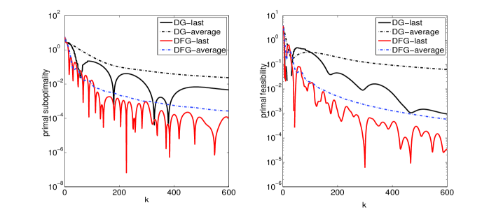
Figure 1: Typical performance in terms of primal suboptimality and infeasibility of Algorithms (DG) in the last iterate (DG-last), (DG) in average (DG-average), (DFG) in the last iterate (DFG-last) and (DFG) in average (DFG-average) for $n=50$.

Table 2: Average number of iterations for $10$ random problems for each dimension $n$ for Algorithms (DG) and (DFG) in the last iterate and in the average of iterates. We observe that dual first order methods perform better in the primal last iterate than in the average of iterates.

Alg./n	$10$	$50$	$10^{2}$	$10^{3}$	$5*10^{3}$	$10^{4}$
$k_{\mathrm{last}}^{\mathrm{DG}}$	$44$	$519$	$621$	$5546$	$7932$	$9207$
$k_{\mathrm{avg.}}^{\mathrm{DG}}$	$504$	$1498$	$3706$	$9830$	$-$	$-$
$k_{\mathrm{last}}^{\mathrm{DFG}}$	$13$	$75$	$92$	$382$	$691$	$1145$
$k_{\mathrm{avg.}}^{\mathrm{DFG}}$	$28$	$88$	$123$	$602$	$1078$	$1981$

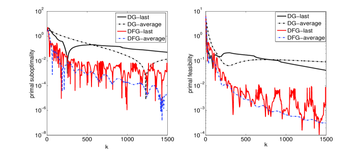
Figure 2: Practical performance comparable with the theoretical estimates for primal suboptimality and infeasibility of Algorithms (DG) in the last iterate (DG-last), (DG) in average (DG-average), (DFG) in the last iterate (DFG-last) and (DFG) in average (DFG-average) for $n=100$.

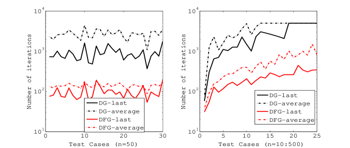
Figure 3: Practical number of iterations of Algorithms (DG) in the last iterate (DG-last), (DG) in average (DG-average), (DFG) in the last iterate (DFG-last) and (DFG) in average (DFG-average) for $30$ random test cases of fixed dimension $n=50$ (left) or variable dimension ranging from $n=10$ to $n=500$ (right).

8.2 Case 2: $\gamma>0,a=0,b\not=0$

In the second set of experiments we choose $(\gamma>0,a=0,b\not=0)$ and simple box constraints $\text{lb}\leq u\leq\text{ub}$ defining the set $U$ (e.g. this optimization model, in separable form, was considered in [27] for resource allocation problems). In this case the objective function is strongly convex and has Lipschitz gradient on $\mathbb{R}^{n}$. Therefore, if the simple box constraints are missing, then according to our theory given in Section 5 Algorithm (DG) is converging linearly.

We first consider box constraints $U=[\text{lb}\;\text{ub}]$ and the results (average number of iterations) are shown in Table 2 for $10$ random problems for each dimension $n$ ranging from $10$ to $10^{4}$. We can again observe that dual first order methods perform better in the primal last iterate than in the average of iterates. Further, we can notice that the behavior of Algorithm (DG) in the last iterate is comparable to that of Algorithm (DFG) in average. However, the inner problem has to be solved with higher accuracy in Algorithm (DFG) than in (DG) since the first one is more sensitive to errors, such as inexact first order information, than the last one (see [11] for a more in depth discussion on inexact dual first order methods).

Table 3: Average number of iterations for $10$ random problems for each dimension $n$ for Algorithms (DG) and (DFG) in the last iterate and in the average of iterates. We can again observe that dual first order methods perform better in the primal last iterate than in the average of iterates.

Alg./n	$10$	$50$	$10^{2}$	$10^{3}$	$5*10^{3}$	$10^{4}$
$k_{\mathrm{last}}^{\mathrm{DG}}$	$35$	$195$	$463$	$782$	$1147$	$2155$
$k_{\mathrm{avg.}}^{\mathrm{DG}}$	$527$	$3423$	$12697$	$-$	$-$	$-$
$k_{\mathrm{last}}^{\mathrm{DFG}}$	$19$	$61$	$97$	$198$	$276$	$292$
$k_{\mathrm{avg.}}^{\mathrm{DFG}}$	$41$	$108$	$186$	$381$	$563$	$582$

Then, we also take $\gamma=0$ and we solve the corresponding QP problems over an increasing dimension $n=10$ to $10^{3}$. In Fig. 4 we compare for Algorithm (DFG) the real number of iterates in the primal latest iterate and average of iterates and the estimated number of iterates ${\cal O}(1/k^{2})$ for a primal suboptimality and infeasibility level of $\varepsilon=10^{-2}$. We observe from Fig. 4 that our theoretical estimates are quite close to the practical ones for the dual fast gradient method.

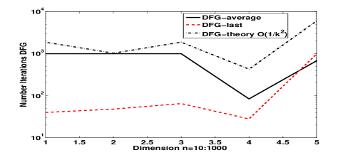
Figure 4: Real number of iterates in the primal latest iterate and average of iterates and the estimated number of iterates ${\cal O}(1/k^{2})$ for Algorithm (DFG).

Finally, we drop the simple box constraints (i.e. now $U=\mathbb{R}^{n}$) and for dimension $n=10^{2}$ we plot in Fig. 5 the behavior of Algorithm (DG) in the last iterate along iterations, starting from $x^{0}=0$. From our results (see Section 5) we have linear convergence, which is also seen in practice from this figure (in logarithmic scale). In the same figure we also plot the theoretical sublinear estimates for the convergence rate of Algorithm (DG) in the last iterate as given in Section 3.1 (see (29) and (3.1)). The plot clearly confirms our theoretical findings, i.e. linear convergence of Algorithm (DG) in the last iterate, provided that $U=\mathbb{R}^{n}$.

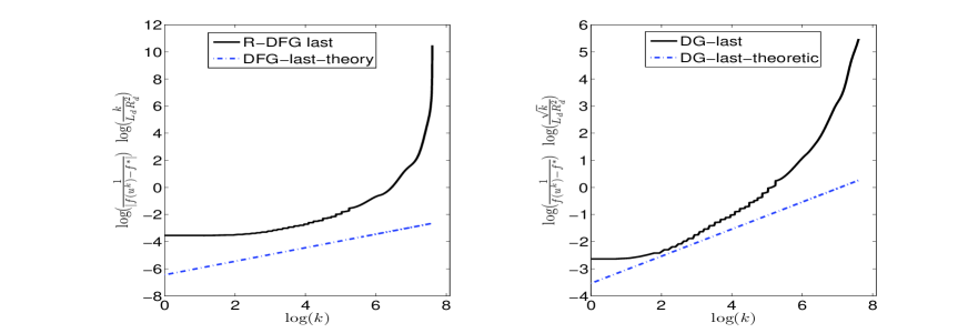
Figure 5: Linear convergence of Algorithms (DG) and (R-DFG) in the last iterate for $U=\mathbb{R}^{n}$: logarithmic scale of primal suboptimality. We also compare with the theoretical sublinear estimates (dot lines) for the convergence rate in the last iterate. The plot clearly shows our theoretical findings, i.e. linear convergence.

References

[1]
A. Beck, A. Nedic, A. Ozdaglar, and M. Teboulle,
Optimal distributed gradient methods for network resource allocation problems,
IEEE Transactions on Control of Network Systems, 1(1):1–10, 2014.
[2]
E. Gustavsson, M. Patriksson, and A.B. Stromberg,
Primal convergence from dual subgradient methods for convex optimization,
Mathematical Programming, Ser. A, 2014.
[3]
M. Hong and Z.Q. Luo,
On the linear convergence of the alternating direction method of
multipliers,
Technical report, University of Minnesota, arxiv.org/abs/1208.3922,
2012.
[4]
F. P. Kelly, A.K. Maulloo, and D.K.H. Tan,
Rate control in communication networks: shadow prices, proportional
fairness and stability,
Journal of the Operational Research Society, 49:237–252, 1998.
[5]
K.C. Kiwiel, T. Larsson, and P.O. Lindberg,
Lagrangian relaxation via ballstep subgradient methods,
Mathematics of Operations Research, 32(3):669–686, 2007.
[6]
G. Lan and R.D.C. Monteiro,
Iteration-complexity of first-order augmented lagrangian methods for convex programming,
Mathematical Programming, 2015.
[7]
T. Larsson, M. Patriksson, and A.B. Stromberg,
Ergodic convergence in subgradient optimization,
Optimization Methods and Software, 9(1–3):93–120, 1998.
[8]
Z.Q. Luo and P. Tseng,
On the convergence of coordinate descent method for convex
differentiable minimization,
Journal of Optimization Theory and Applications, 72(1):7–35, 1992.
[9]
Z.Q. Luo and P. Tseng,
On the convergence rate of dual ascent methods for
linearly constrained convex minimization,
Mathematics of Operations Research, 18(4):846–867, 1993.
[10]
I. Necoara and V. Nedelcu,
On linear convergence of a distributed dual gradient algorithm for
linearly constrained separable convex problems,
Automatica, in press:1–9, 2015.
[11]
I. Necoara and V. Nedelcu,
Rate analysis of inexact dual first order methods: application to dual decomposition,
IEEE Transactions on Automatic Control, 59(5):1232 –1243, 2014.
[12]
I. Necoara and J.A.K. Suykens,
Application of a smoothing technique to decomposition in convex optimization,
IEEE Transactions on Automatic Control, 53(11):2674–2679, 2008.
[13]
I. Necoara and J.A.K. Suykens,
An interior-point lagrangian decomposition method for separable convex optimization,
Journal of Optimization Theory and Applications, 143(3):567–588, 2009.
[14]
V. Nedelcu, I. Necoara, and Q. Tran Dinh,
Computational complexity of inexact gradient augmented lagrangian methods: application to constrained MPC,
SIAM Journal on Control and Optimization, 52(5):3109–3134, 2014.
[15]
A. Nedic and A. Ozdaglar,
Approximate primal solutions and rate analysis for dual subgradient methods,
SIAM Journal on Optimization, 19(4):1757–1780, 2009.
[16]
Y. Nesterov,
Introductory Lectures on Convex Optimization: A Basic Course,
Kluwer, Boston, USA, 2004.
[17]
Y. Nesterov,
Smooth minimization of non-smooth functions,
Mathematical Programming, 103(1):127–152, 2005.
[18]
Y. Nesterov,
How to make the gradients small,
Optima, 88:10–11, 2012.
[19]
Y. Nesterov,
Gradient methods for minimizing composite functions,
Mathematical Programming,
140(1):125–161, 2013.
[20]
P. Patrinos and A. Bemporad,
An accelerated dual gradient-projection algorithm for embedded linear model predictive control,
IEEE Transactions on Automatic Control, 59(1):18–33, 2014.
[21]
R.T. Rockafellar and R.J. Wets,
Variational Analysis,
Springer-Verlag, New York, 1998.
[22]
A. Beck and M. Teboulle,
A fast dual proximal gradient algorithm for convex minimization and applications,
Operations Research Letters, 42(1):1–6, 2014.
[23]
P. Tseng,
On accelerated proximal gradient methods for convex-concave optimization,
SIAM Journal of Optimization, submitted:1–20, 2008.
[24]
P. Tseng,
Approximation accuracy, gradient methods and error bound for structured convex optimization,
Mathematical Programming, 125(2):263–295, 2010.
[25]
P.W. Wang and C.J. Lin,
Iteration complexity of feasible descent methods for convex optimization,
Journal of Machine Learning Research, 15:1523–1548, 2014.
[26]
E. Wei, A. Ozdaglar, and A. Jadbabaie,
A distributed newton method for network utility maximization –
Part I and II,
IEEE Transactions on Automatic Control, 58(9), 2013.
[27]
L. Xiao and S. Boyd,
Optimal scaling of a gradient method for distributed resource allocation,
Journal of Optimization Theory and Applications, 129(3), 2006.
[28]
R.D. Zimmerman, C.E. Murillo-Sanchez, and R.J. Thomas,
Matpower: Steady-state operations, planning, and analysis tools for power systems research and education,
IEEE Transactions on Power Systems, 26(1):12–19, 2011.