Accurate, fully-automated NMR spectral profiling for metabolomics

Abstract

Many diseases cause significant changes to the concentrations of small molecules (a.k.a. metabolites) that appear in a person’s biofluids, which means such diseases can often be readily detected from a person’s “metabolic profile”.This information can be extracted from a person’s biofluids using nmr spectroscopy. Today, this is often done manually by trained experts, which means this process is relatively slow, expensive and can be error-prone. A system that can quickly, accurately and autonomously produce a person’s metabolic profile would enable efficient and reliable prediction of many such diseases from a single sample, which could significantly improve the way medicine is practiced.

This paper presents such a system: Given a 1D ¹H nmr spectrum of a complex biofluid such as serum or CSF, our bayesil system can automatically determine this metabolic profile, and do so without any human guidance. This requires first performing all of the required spectral processing steps (i.e., Fourier transformation, phasing, solvent-removal, chemical shift referencing, baseline correction, lineshape convolution) then matching this resulting spectrum against a reference compound library, which contains the “signatures” of each relevant metabolite. Many of these processing steps are novel algorithms, and our matching step views spectral matching as an inference problem within a probabilistic graphical model that rapidly approximates the most probable metabolic profile.

Our extensive studies on a diverse set of complex mixtures (real biological samples, defined mixtures and realistic computer generated spectra; each involving $\sim 50$ compounds), show that bayesil  can autonomously and accurately find nmr-detectable metabolites at concentrations as low as $2\mu$M, in terms of both identification ($\sim 90\%$ correct) and quantification ($\sim 10\%$ error), in under 5 minutes on a single CPU processor. These results demonstrate that bayesil  is the first fully-automatic publicly-accessible system that provides quantitative nmr spectral profiling effectively – with an accuracy that meets or exceeds the performance of highly trained human experts. We anticipate this tool will usher in high-throughput metabolomics and enable a wealth of new applications of NMR in clinical settings. Users can access bayesil at http://www.bayesil.ca.

Metabolomics is a relatively new branch of “omics” science that focuses on the system-wide characterization of metabolites [1]. Metabolomics is often viewed as complementary to the other “omics” fields as it provides information about both an organism’s phenotype and its environment. Because metabolomics provides a unique window on gene-environment interactions, it is playing an increasingly important role in many quantitative phenotyping and functional genomics studies [2, 3, 4]. It is also finding more applications in disease diagnosis, biomarker discovery and drug development/discovery (e.g., [5, 6, 7]). This rapid growth in interest and excitement surrounding metabolomics is also revealing its “Achilles heel”: Unlike proteomics, genomics or transcriptomics, which are high-throughput sciences, metabolomics is a relatively low-throughput science. Compared to genomics, where it is now possible to automatically characterize 1000s of genes, 100’s of thousands of transcripts and millions of snps in mere minutes, metabolomics only allows users to identify and measure a few dozen metabolites after many hours of manual effort. In other words, metabolomics is not automated. This problem may stem from the history of metabolomics, as its analytical techniques, such as nmr spectroscopy, gas-chromatography-mass spectrometry (gc-ms) and liquid chromatography-mass spectrometry (lc-ms), were originally developed for identifying and quantifying pure compounds, not complex mixtures. Because most biological samples contain hundreds of metabolites, the resulting nmr, hplc or lc-ms spectra usually contain hundreds or even thousands of peaks. The challenge in metabolomics, therefore, is to identify the mixture of compounds that produced this forest of peaks. This compound identification process, called spectral profiling, involves fitting the mixture spectrum to a set of individual pure reference spectra obtained from known compounds [8, 9]. If done correctly, the fitting process yields not only the identity of the compounds, but also the concentration of those compounds. Therefore, the end result of a successful spectral profiling study is a table of metabolite names and their absolute or relative concentrations. Because spectral profiling is such a complex pattern recognition problem, it is often best done by a trained expert. However, this reliance on manual data analysis by a human expert is problematic, as it is slow and leads to inconsistent results, operator errors and reduced levels of reproducibility [10].

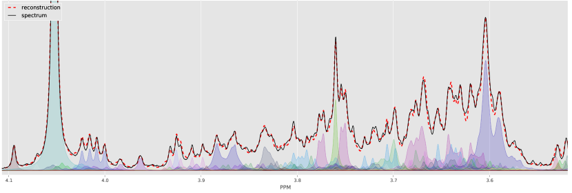
Figure 1: This figure shows the crowded region (3.5-4.1 ppm) of a computer generated spectrum with 150 compounds (solid black) and the fit produced by bayesil (dashed red) as well as individual clusters as quantified by bayesil. Each cluster is free to shift a specified amount, which is at least 0.025 ppm.

The automation bottleneck in metabolomics is widely recognized, and has led to a number of efforts to accelerate or automate compound identification and/or quantification in lc-ms, in gc-ms and in nmr spectroscopy. Some of the most active efforts in (semi)automated compound identification and quantification have been in nmr-based metabolomics. In particular, several software packages have been developed that support semi-automatic nmr spectral profiling of 1D and 2D ¹h nmr spectra, including some commercial packages (e.g., [12, 14, 13]). There are tremendous differences in the quantification/identification capabilities, spectral database size, speed and instrument compatibility of these software tools. Furthermore, these packages either require manual fitting or manual spectral processing, or a bit of both; see Appendix I for a comprehensive list of nmr softwares and their limitations. The need for such manual interventions leads to a number of issues, including slower throughput, operator fatigue and associated operator errors, the need for highly trained and dedicated experts, the requirement of two or more spectral assessments for quality assessment and control purposes, and inconsistent results between individuals, between labs or over different time periods [8, 10].

It would be better to have a software system that can automatically perform both spectral processing and spectral deconvolution, be able to analyze complex mixtures ($\sim$60 compounds) quickly and accurately, and be able to produce reliable compound concentrations. Here we describe such a system, called bayesil.

Extensive testing, on computer-generated and laboratory-generated chemical mixtures as well as real biological samples, shows that bayesil consistently performs with $\sim 90\%$ accuracy for compound identification in mixtures with up to $60$ different metabolites. It also determines metabolite concentrations with $\sim 10\%$ error. For computer-generated biofluid spectra, where the ground truth is known, bayesil consistently outperforms highly trained experts in both identification and quantification. bayesil appears to be the first system that supports fully automated and fully quantitative nmr-based metabolomics. This paper describes this system, its underlying algorithms and its performance across various tests.

I Metabolic profiling pipeline

bayesil performs fully automated spectral processing and spectral profiling for 1D ¹h nmr spectra collected on either Agilent/Varian or Bruker instruments, at several different frequencies. In particular, it uses a variety of intelligent phasing and baseline correction methods to automatically process raw 1D nmr spectra (i.e., FIDs). It also uses approximate inference techniques to rapidly perform very accurate spectral deconvolution, yielding both compound identities and their concentrations. Here we briefly describe bayesil’s spectral processing algorithms, the principles and rationale behind bayesil’s spectral deconvolution method and the construction of bayesil’s spectral library.

I-A Spectral Processing in BAYESIL

Successful nmr spectral profiling depends critically on the quality and uniformity of the starting nmr spectrum. Unfortunately, most spectral processing functions (i.e., phasing, baseline correction, solvent filtering, chemical shift referencing) are left to the user. Given the complexity and large number of variables, values and filters that can be used, many view spectral processing more as an art, rather than a science. Different perspectives or different personal thresholds on what is a “good looking” nmr spectrum can potentially lead to very different results regarding what compounds are identified or which compounds are accurately quantified in a biofluid spectrum. To address this issue, bayesil itself performs all of the spectral processing functions: starting from the FID, it performs zero-filling, Fourier and Hilbert transformation, phasing, baseline correction, chemical shift referencing, reference deconvolution and smoothing. Automating this process ensures reproducibility, consistency and uniformity of the input data prior to spectral deconvolution. Here we briefly sketch some of the more challenging steps in this process.

Phasing involves maximizing the symmetry of the peaks by reducing zero-order and first-order phase mismatch. Zero-order phase mismatch is a sign of the difference between the reference phase and the receiver phase and is independent of frequency. The first-order phase mismatch can be a result of the time-delay between excitation and detection, flip-angle variation and the filter that is used to reduce the noise outside of the spectral bandwidth [15]. In addition to using well-known techniques, such as spectral norm minimization [16], bayesil uses the cross entropy optimization method [11] to jointly maximize a direct measure of peak symmetry for isolated peaks across the spectrum.

Baseline correction involves removing distortions that may arise from hardware artifacts or highly concentrated components of the mixture (e.g., solvent), while keeping the desirable signal intact. This process is often performed in two steps: 1) baseline-detection and 2) modelling. bayesil relies on iterative thresholding [17] and estimating the signal-to-noise ratio to detect the baseline points. It uses monotonic cubic Hermite interpolation [18] and Whittaker smoothing technique for baseline modelling [19].

bayesil also provides the options for smoothing and line-broadening using Savitzky-Golay [20] and Gaussian filters. However smoothing is mostly cosmetic and it is not essential for spectral deconvolution. In fact, it may degrade the signal and occasionally remove the the low-amplitude and narrow peaks. Similarly, we found the effect of reference deconvolution – which may be used to remove instrumental or experimentally induced distortions of the Lorentzian lineshape – is also mostly cosmetic, and if the distortion around the reference peak has any source other than poor shimming, using reference deconvolution will have an adverse effect on the rest of the nmr spectrum.

I-B Spectral Deconvolution

An nmr spectrum for a compound ${\scriptstyle{\mathcal{M}}}$ is a collection of one or more Lorentzian peaks formed into one or more clusters – that is, each compound ${\scriptstyle{\mathcal{M}}}$ is a set of clusters $\{{\scriptstyle{\mathcal{C}}}_{k}\}$, where each cluster ${\scriptstyle{\mathcal{C}}}_{k}$ is set of peaks, and each peak is defined by a triple, $\boldsymbol{\theta}=(\theta_{1},\theta_{2},\theta_{3})$ corresponding to its height, center and width (at half height) respectively – where the height at $x$ due to this peak is $\mathsf{q}(x;\boldsymbol{\theta})=\frac{\theta_{1}\theta_{3}}{\theta_{3}+4(\theta_{2}-x)^{2}}$. Letting ${\mathcal{X}}$ refer to the entire spectrum (e.g., from -1 to 13 ppm when referenced against the DSS peak), the height of the spectrum of a pure compound ${\scriptstyle{\mathcal{M}}}$ at each location $x\in{\mathcal{X}}$, is

$$\widehat{\mathsf{s}}{(x\,;{\scriptstyle{\mathcal{M}}},\rho_{\scriptstyle{\mathcal{M}}},\boldsymbol{\delta}_{\scriptstyle{\mathcal{M}}})}\quad=\quad\rho_{\scriptstyle{\mathcal{M}}}\sum_{{\scriptstyle{\mathcal{C}}}\in{\scriptstyle{\mathcal{M}}}}\ \sum_{\boldsymbol{\theta}\in{\scriptstyle{\mathcal{C}}}}\mathsf{q}(x-\delta_{\scriptstyle{\mathcal{C}}};\boldsymbol{\theta})$$ (1)

where $\rho_{\scriptstyle{\mathcal{M}}}$ is the concentration of this compound and $\delta_{\scriptstyle{\mathcal{M}}}=\{\delta_{{\scriptstyle{\mathcal{C}}}}\,|\,{\scriptstyle{\mathcal{C}}}\in{\scriptstyle{\mathcal{M}}}\}$ is the set of chemical shifts for the clusters associated with this compound.

An nmr spectrum is essentially a linear combination of the peaks in its component compounds: that is, the height at each ppm value $x$ of a mixture spectrum is just the sum of the contributions of each compound. This means, given the concentrations of the compounds $\boldsymbol{\rho}=\{\rho_{\scriptstyle{\mathcal{M}}}\}$, and the chemical shifts $\boldsymbol{\delta}=\bigcup_{\scriptstyle{\mathcal{M}}}\boldsymbol{\delta}_{{\scriptstyle{\mathcal{M}}}}$ of the clusters associated with these compounds, we can then “draw” an nmr spectrum – i.e., the height at each ppm $x$, given this $\boldsymbol{\rho}$ and $\boldsymbol{\delta}$, is $\widehat{\mathsf{s}}{(x\,;\boldsymbol{\rho},\boldsymbol{\delta})}\ =\ \sum_{{\scriptstyle{\mathcal{M}}}}\widehat{\mathsf{s}}{(x\,;{\scriptstyle{\mathcal{M}}},\rho_{\scriptstyle{\mathcal{M}}},\boldsymbol{\delta}_{\scriptstyle{\mathcal{M}}})}$.

The spectral deconvolution challenge, in general, is the reverse process: Given a set of compounds $\{{\scriptstyle{\mathcal{M}}}_{1},\ldots,{\scriptstyle{\mathcal{M}}}_{r}\}$ with associated signatures (i.e., $\boldsymbol{\theta}$ values of their peaks, organized in clusters) and the observed spectrum $\mathsf{s}(\cdot)$, find the “best” combination of concentrations $\boldsymbol{\rho}$ and shifts $\boldsymbol{\delta}$ to fit that spectrum. To determine which values are best, for now, we consider a simple loss function that is the (square of the) difference of the heights between the observed spectrum $\mathsf{s}(\cdot)$ and the reconstructed spectrum $\widehat{\mathsf{s}}{(\cdot\,;\boldsymbol{\delta},\boldsymbol{\rho})}$

$$\mathsf{\ell}_{{\mathcal{X}}}\left(\ \mathsf{s}(\cdot),\ \widehat{\mathsf{s}}{(\cdot\,;\boldsymbol{\rho},\boldsymbol{\delta})}\ \right)\;=\;\int_{x\in{\mathcal{X}}}\big{(}\,\mathsf{s}(x)-\widehat{\mathsf{s}}{(x\,;\boldsymbol{\rho},\boldsymbol{\delta})}\,\big{)}^{2}\,\mathrm{d}x$$ (2)

where the subscript ${\mathcal{X}}$ indicates that this loss function applies to the entire spectrum; see Appendix II for bayesil’s actual loss function.

Our task is to find the values of

$$[\boldsymbol{\rho}^{*},\ \boldsymbol{\delta}^{*}]\quad=\quad\arg_{\boldsymbol{\rho},\boldsymbol{\delta}}\min\quad\mathsf{\ell}_{{\mathcal{X}}}\left(\mathsf{s}(\cdot),\,\widehat{\mathsf{s}}{(\cdot\,;\boldsymbol{\rho},\boldsymbol{\delta})}\right)$$ (3)

that minimize this loss function. Figure 1 shows part of a spectrum over a complex mixture, and bayesil’s solution obtained by minimizing the loss function.

This corresponds to search over a huge space – all possible shifts for each of the clusters, and all possible concentrations over the compounds. The key innovation of bayesil is how it minimizes this highly non-linear loss function, efficiently. In particular, bayesil “factors” this large task into a set of inter-related smaller tasks. Two characteristics of the nmr spectra make this factorization possible: 1) each shift is over only a small range (typically a window of $\pm 0.025$ ppm); and 2) as the height in the spectrum due to a Lorentzian peak diminishes quadratically from its center, each peak and therefore each cluster can only “influence” a small interval; see Appendix III.

Now consider a function that maps each point in the spectrum to the set of clusters that might affect the height at this location. That is, given the set of compounds $\{{\mathbf{\scriptstyle{\mathcal{M}}}}\}$ that might appear in a particular biofluid (e.g., the 48 that can appear in CSF), we can identify each ppm location $x\in{\mathcal{X}}$ with the small set of clusters that might influence it, ${\mathbf{\scriptstyle{\mathcal{C}}}}(x)$.

We can then partition the spectrum into disjoint contiguous regions, $\{{\mathcal{X}}_{I}\}$, where every ppm location in each ${\mathcal{X}}_{I}$ involves exactly the same subset of clusters – i.e., for any pair of points $x_{1},x_{2}\in{\mathcal{X}}_{I}$, we know that ${\mathbf{\scriptstyle{\mathcal{C}}}}(x_{1})={\mathbf{\scriptstyle{\mathcal{C}}}}(x_{2})$. For example, our library for CSF includes 48 compounds, with a total of 180 clusters and 946 peaks. A typical CSF spectrum is partitioned into $\sim$350 regions. Each of these regions will involve between 1 and $\sim$25 clusters, and span between 0.0001 and 1.5 ppm. Moreover, each cluster will appear in between 1 and $\sim$70 different regions.

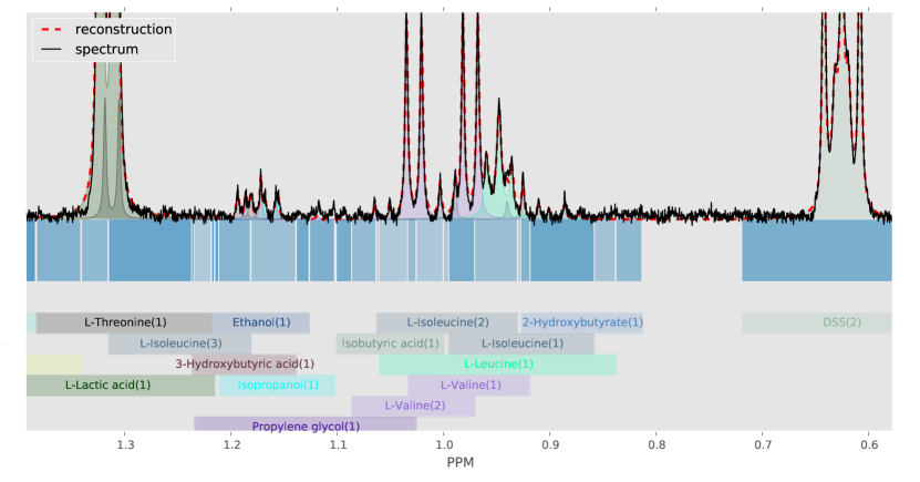
Figure 2: Partitioning of ${\mathcal{X}}$ into continuous blocks ${\mathcal{X}}_{I}\subset{\mathcal{X}}$ for a part of a human serum spectrum. Here each block is shown with a different shade of blue, below the horizontal axis. The domain of influence of each cluster is also indicated with coloured blocks.

Figure 2 shows the division of a part of human serum nmr spectrum into regions ${\mathcal{X}}_{I}$; blocks in different shades of blue. For example the region ${\mathcal{X}}_{[.8563,9289]}$ from 0.8563 to 0.9289 ppm might include significant contributions from the first cluster of 2-Hydroxybutyrate, the first cluster of L-Isoleucine and/or the first cluster of L-Leucine. The region immediately to its left (from 0.9289 to 0.9370 ppm) includes these and also a cluster of L-Valine, and the one to the right (from 0.8563 to 0.87526 ppm) does not include L-Isoleucine.

As the loss function $\mathsf{\ell}(\cdot,\cdot)$ is additive over the domain ${\mathcal{X}}$, we can rewrite the optimization of eq[3] as the sum of the losses for each of the regions ${\mathcal{X}}_{I}$:

$$[\boldsymbol{\rho}^{*},\boldsymbol{\delta}^{*}]\;=\;\arg_{\boldsymbol{\rho},\boldsymbol{\delta}}\min\sum_{I}\mathsf{\ell}_{{\mathcal{X}}_{I}}\big{(}\,\mathsf{s}(\cdot),\widehat{\mathsf{s}}{(\cdot\,;\boldsymbol{\rho}_{I},\boldsymbol{\delta}_{I})}\,\big{)}$$ (4)

Now recall that each region ${\mathcal{X}}_{I}$ involves relatively few compounds and clusters. This suggests a preliminary step of simply “solving” each region, by itself: i.e., find the best centers for the clusters in that region $\boldsymbol{\delta}_{I}$, and the best concentrations for the associated compounds $\boldsymbol{\rho}_{I}$, which collectively minimize the loss over the ppm-interval ${\mathcal{X}}_{I}$. This simple approach is fast, as it involves relatively few variables and a limited range of ppm-values. Unfortunately, this does not produce the overall correct answer – that is, each region has an opinion about the concentration and shift values of its cluster, and when two (or more) regions each involve the same variable, they must both agree on its value.

Figure 3: Factor-graph for a library of 15 compounds immediately below an associated nmr spectrum. Each factor is represented by a square and each variable using a circle. Concentration (larger circles) and shift variables (smaller circles, beside the associated concentration) corresponding to each compound appear together. The position of each factor $\mathsf{f}_{I}$ position in the plot corresponds to the center of the corresponding block ${\mathcal{X}}_{I}$.

To address this problem, we take a probabilistic approach, viewing the task of minimizing the loss function eq[2] as finding the “Maximum a Posteriori” (MAP) assignment – i.e., the assignment to all of the cluster-shift and compound-concentration $[\boldsymbol{\delta},\boldsymbol{\rho}]$ variables that makes the observed data as likely as possible. Here, the Boltzmann formula gives the probabilistic interpretation of the loss (a.k.a.  the energy)

$$\mathbb{P}(\,\boldsymbol{\rho},\boldsymbol{\delta}\,|\,\mathsf{s}(\cdot)\,)=\frac{1}{Z}\exp\left\{-\frac{1}{T}\mathsf{\ell}_{{\mathcal{X}}}\big{(}\,\mathsf{s}(\cdot),\,\widehat{\mathsf{s}}{(\cdot\,;\boldsymbol{\rho},\boldsymbol{\delta})}\,\big{)}\right\}$$ (5)

where $Z$ is the normalization constant and $T$ is known as the “temperature” parameter, explained in Appendix IV. Using the decomposition of loss over regions (eq[4]) we can write this distribution in factored form

$$\mathbb{P}(\,\boldsymbol{\rho},\boldsymbol{\delta}\,|\,\mathsf{s}(\cdot)\,) =\frac{1}{Z}\prod_{I}\mathsf{f}_{I}(\boldsymbol{\rho}_{I},\boldsymbol{\delta}_{I})$$

$$\mathsf{f}_{I}(\boldsymbol{\rho}_{I},\boldsymbol{\delta}_{I}) =\exp\bigg{\{}\;-\frac{1}{T}\mathsf{\ell}_{{\mathcal{X}}_{I}}\big{(}\,\mathsf{s}(\cdot),\,\widehat{\mathsf{s}}(.;\boldsymbol{\rho}_{I},\boldsymbol{\delta}_{I})\,\big{)}\;\bigg{\}}$$ (6)

This decomposition of the distribution $\mathbb{P}(\,\boldsymbol{\rho},\boldsymbol{\delta}\,|\,\mathsf{s}(\cdot)\,)$ can be represented using a probabilistic graphical model, known as a factor graph [21], which is a graph with two types of nodes: 1) factors (corresponding to regions or $\mathsf{f}_{I}$), and 2) variables (here, concentrations and chemical shifts). Each factor has arcs that point only to its associated variables. Figure 3 shows a portion of this factor-graph for a simple defined mixture of 15 compounds.

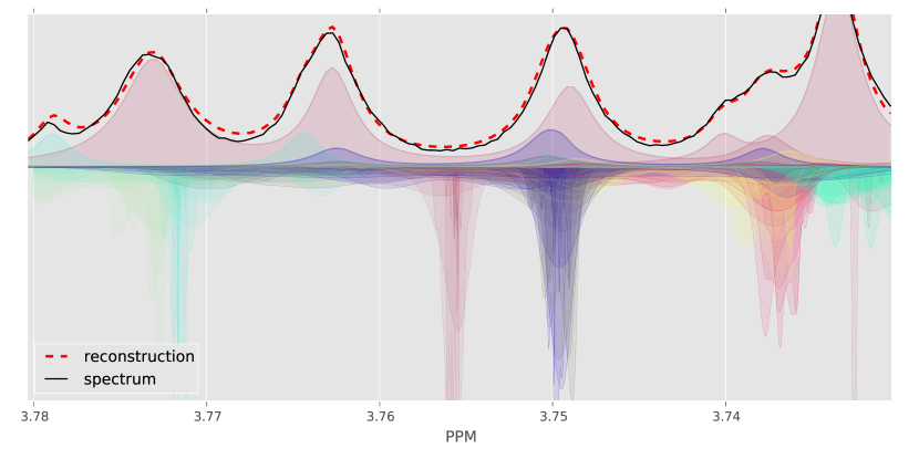
Figure 4: A small region of human serum spectrum. The plots above horizontal axis show the original spectrum (solid black), individual clusters as well as overall fit (dashed red). The curves below horizontal axis show the bayesil’s distribution over chemical shift variables for each cluster (${\scriptstyle{\mathcal{C}}}$), over $6$ iterations of spectral deconvolution. The distributions become more peaked towards the correct center in each iteration. Distributions below the horizon have the color of their associated cluster.

By formulating the spectral deconvolution problem as MAP inference in a factor-graph, we have a variety of inference techniques at our disposal [21]. bayesil uses a non-parametric sequential Monte Carlo method [22] tailored to this inference problem (see Appendix IV for details). Using a Gaussian distribution around a set of particles (a.k.a.  kernel density estimation) bayesil represents a distribution over each concentration $\rho_{\scriptstyle{\mathcal{M}}}$ and shift variable $\delta_{\scriptstyle{\mathcal{C}}}$. By reducing the temperature parameter, these distributions are gradually narrowed in each iteration until convergence, at which point the mode of the distributions represent an approximate MAP assignment. Figure 4 shows the evolution of distributions over the chemical shift variables over $6$ iterations of spectral deconvolution.

I-C BAYESIL’s Spectral Library

Key to the success of any spectral deconvolution algorithm is the quality and size of its spectral library. We therefore collected 1D ¹h nmr reference spectra for each of the compounds in bayesil’s spectral library using pure compounds obtained from the Human Metabolome Library [1], using a standard protocol (see Materials and Methods). The spectral library contains relevant information about each compound (${\scriptstyle{\mathcal{M}}}$) including individual peak clusters (${\scriptstyle{\mathcal{C}}}$) and peak amplitude positions and widths (i.e., $\boldsymbol{\theta}$ in eq[1]), as well as allowable chemical shift window $\underline{\delta}_{\scriptstyle{\mathcal{C}}}\leq\delta_{\scriptstyle{\mathcal{C}}}\leq\overline{\delta}_{\scriptstyle{\mathcal{C}}}$ for each cluster ${\scriptstyle{\mathcal{C}}}$.

To analyze each biofluid, bayesil uses a specific spectral sub-library – here, one for serum and another one for CSF. The serum library consists of 50 nmr-detectable compounds from the human serum metabolome [23] while the CSF library consists of the 48 nmr-detectable compounds from the human CSF metabolome [24]; see Appendix V. The use of biofluid-specific or organism-specific spectral libraries significantly improves the performance of the spectral fitting process as it reduces the number of possible explanations for each peak.

II Assessment

bayesil was assessed using 3 different types of spectral data sets over two different types of biofluids:
(a) Computer generated mixtures derived from its spectral library. We generated 5 random serum and 5 random CSF spectra by sampling from the distribution of the measured concentration ranges of various compounds, and the probability of observing them in the mixture from [23, 24]. The chemical shifts were also randomly sampled according to the chemical shift ranges from the corresponding spectral libraries. To be more realistic, we also added a small amount of noise to the spectrum – independently to the height at each position $x\in{\mathcal{X}}$. These correspond to “perfect” spectra, and are intended to assess the robustness and performance limits of bayesil under optimal conditions.
(b) Defined mixtures prepared in the laboratory. We created 15 defined mixtures (5 defined mixture of serum, 5 defined mixture of CSF, 5 random mixture of compounds in both serum and CSF, involving $>60$ compounds), using carefully measured pure compounds and freshly prepared solutions. These provide real spectral data that probably include common spectral and solution artifacts (baseline and phasing issues, minor spontaneous reaction products, contaminants, matrix or pH effects). This set was used to assess bayesil’s performance under well-controlled conditions where the composition and of the mixtures was almost perfectly known.
(c) Biological serum and CSF samples. We took human CSF and serum samples from previously studied samples that had been analyzed and quantified by nmr experts – here, 50 human serum and 5 human CSF samples. The set of compound mixtures was used to assess bayesil’s performance under realistic conditions with common spectral and solution artifacts. Although human CSF contains a smaller number of nmr-detectable compounds than human serum, it is more difficult to profile due to the lower concentration of metabolites. While both the biological samples and defined mixtures were thoroughly analyzed, their exact compound concentrations cannot be perfectly known.
Overall, we believe these 3 test sets provide a robust assessment of bayesil’s performance (as well as its limitations) under a wide range of conditions.

TABLE I: Identification and quantification accuracy of bayesil and human expert on various data-sets.

bayesil estimates the “detection threshold” based on the signal to noise ratio (snr) in each spectrum – i.e., when the signal is noisy this threshold is increase to provide a more confident identification and quantification. The snr and therefore the detection threshold is directly related to the number of scans during spectral acquisition. For example our biological serum samples are produced using $128$ scans and therefore most detection thresholds are $\sim 10\mu$M. Since compound concentrations in our CSF samples are considerably lower than serum, their analysis requires higher quality spectra (see Materials and Methods). Our CSF samples use $1024$ scans resulting in detection thresholds that are often less than $2\mu$M. However this threshold is not uniform across metabolites. bayesil also uses a relative factor in compound detectability; as some compound such as Choline are easy to identify and quantify at low concentrations while for some other compounds such as L-Asparagine, experts use a higher detection threshold.

Given a spectrum of a mixture of compounds (with “true” concentrations $\{{\rho}_{{\scriptstyle{\mathcal{M}}}}\}$), bayesil returns its estimates of these concentrations $\{\widehat{\rho}_{{\scriptstyle{\mathcal{M}}}}\}$, which might be 0 if that compound is absent. We say a compound is a true positive if both $\widehat{\rho}_{{\scriptstyle{\mathcal{M}}}}$ and $\rho_{{\scriptstyle{\mathcal{M}}}}$ are positive – that is, greater than the detection threshold, and a true negative if both $\widehat{\rho}_{{\scriptstyle{\mathcal{M}}}}$ and $\rho_{{\scriptstyle{\mathcal{M}}}}$ are less than the threshold; in either case, bayesil’s prediction is considered correct. bayesil’s identification accuracy for a given spectrum is the ratio of correct labels (true positives plus true negatives) to the library size. bayesil’s “quantitative accuracy” describes how often its estimates $\widehat{\rho}_{{\scriptstyle{\mathcal{M}}}}$ were “close enough” to the true values $\rho_{{\scriptstyle{\mathcal{M}}}}$; note that simply computing $|\widehat{\rho}_{{\scriptstyle{\mathcal{M}}}}-{\rho}_{{\scriptstyle{\mathcal{M}}}}|$ is not enough as this measure would basically only consider the compounds with high concentrations. We instead use the $\mathrm{median}_{{\scriptstyle{\mathcal{M}}}}\left(\frac{|\rho_{\scriptstyle{\mathcal{M}}}-\widehat{\rho}_{\scriptstyle{\mathcal{M}}}|}{\max(\widehat{\rho}_{\scriptstyle{\mathcal{M}}},\rho_{\scriptstyle{\mathcal{M}}})}\right)$ as a measure of the percentage error in concentrations. Table I reports bayesil’s identification and quantification accuracies, for each of the tasks listed above. For the biological and synthetic samples, we assume the human expert’s assessment is correct.

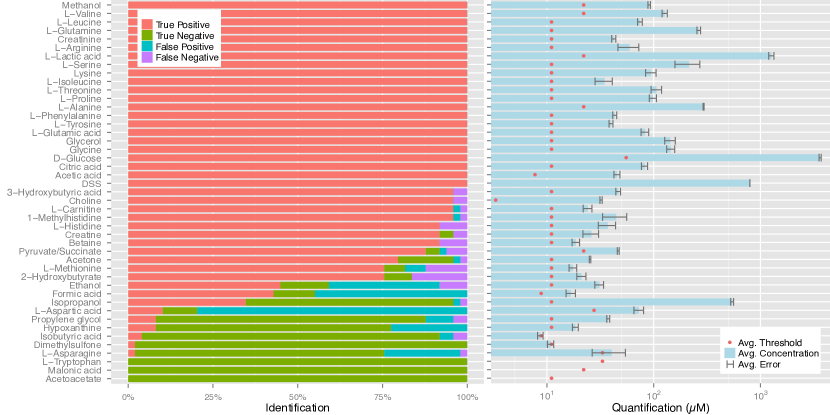
Figure 5: (left) bayesil’s true/false positive/negative rate in identification of individual compounds in 50 biological serum samples. (right) The average concentration for correctly identified compounds in the same samples. The error bars show the average difference between bayesil and expert values for each compound and the red dots show the detection threshold for each compound.

Figure 5(left) reports the frequency of false/true positives/negatives for individual compounds in 50 serum samples. Figure 5(right) shows the average of $\rho_{\scriptstyle{\mathcal{M}}}$ for correctly identified compounds in 50 serum samples, as reported by nmr experts, the average detection threshold for diffent compounds as well as the average difference $\widehat{\rho}_{{\scriptstyle{\mathcal{M}}}}-\rho_{{\scriptstyle{\mathcal{M}}}}$, between bayesil and expert’s estimate for each compound.

These results on a diverse set of test data suggest that bayesil is often within $10\%$ of the expert’s estimate, and where the ground truth is known, bayesil’s metabolic profile is often more accurate than the expert’s. bayesil’s web-page http://www.bayesil.ca provides a complete description of all of the studies reported above, showing the fits and the metabolic profiles obtained.

II-A Efficiency

On a single 2.8 GHz CPU processor, bayesil typically takes less than 5 minutes to profile a serum or CSF spectrum. Over a sustained 24 hour period, bayesil should be able to process more than 200 spectra (vs. $\sim$20 spectra/day for a human expert) and accurately identify-&-quantify approximately 50 compounds per spectrum. This corresponds to an output of more than 5000 metabolite measurements a day for a single CPU. It is possible to produce profiles yet faster by reducing the number of particles used in bayesil’s deconvolution process: reducing this by a factor of 10, reduces the run-time to less than one minute. This speed-up often reduces the identification and quantification accuracy by only 5-10%.

II-B Limitations

A key disadvantage of nmr analysis (versus mass spec), in general, is that nmr is relatively insensitive, with a lower limit of detection of $\sim 1-5$ $\mu$M and a requirement of relatively large sample sizes ($\sim 500\mu L$). For high-quality spectra with high snr, such as CSF samples in our study, bayesil is often able to achieve its high accuracy within these detection limits.

Key to the high level of performance of bayesil is the use of biofluid-specific spectral libraries in its spectral fitting routines (a.k.a. targeted profiling). Without these, bayesil would be substantially slower and less accurate in both identification and quantification. Therefore users must provide bayesil with information about the biofluid being analyzed. Obviously, the mis-identification or mislabelling of a biofluid sample could lead to somewhat poorer results.

This need for prior knowledge about the typical composition of biofluid mixtures has motivated us, and others, to spend considerable efforts to determine the nmr-detectable metabolomes for many biofluids, including human plasma/serum, cerebrospinal fluid, saliva and urine (e.g., [23, 24, 25]), milk and rumen (e.g., [26]), cell extracts (e.g., [27]), cancer cells [28, 29], and many other fluids or extracts.

II-C Other systems

There have been a number of software packages recently developed to facilitate spectral profiling and compound identification/quantification by nmr; see Appendix I for details. However, they do not seem to be particularly accurate on real biofluids. Furthermore, many of the packages are not currently publicly available. To date, the largest number of metabolites that has been automatically identified and quantified using publicly available software is 26 compounds, by batman [13]. However, an analysis of this magnitude required several hours of CPU time to process a single spectrum. Furthermore, batman also requires a human expert to perform many of the preliminary steps. We compared bayesil to batman on simple computer-generated mixtures, involving 5, 10 and 20 compounds selected from batman’s library, as well as a preprocessed human serum sample. For the computer generated spectra, both batman and bayesil used identical libraries containing only the relevant compounds. batman achieved $85-87\%$ quantification accuracy for the computer-generated mixtures but took 2-9 hours to run, while in all cases bayesil achieved $>98\%$ accuracy in less than 3 minutes. For the serum spectra, bayesil used a library of 50 compounds, while batman used a subset of 40 compounds that its library has in common with the serum metabolome. batman took 19 hours to analyze the serum spectrum and identified all the compounds in its library (resulting in $85\%$ identification accuracy) and only $8\%$ quantification accuracy compared to bayesil  which took 5 minutes to achieve $98\%$ identification and $90\%$ quantification accuracy.

Conclusion

nmr is a particularly appealing platform for conducting metabolomic studies on biofluids as it is a rapid, robust, highly reproducible, non-destructive, and fully quantitative technique that requires no prior compound separation or derivatization. The main barrier preventing widespread adoption of NMR-based metabolomics in industrial or clinical applications is the requirement for manual spectral profiling. bayesil addresses this critical problem by providing fully automated spectral processing and deconvolution. Furthermore it is able to perform this task on mixtures containing $>50$ compounds, with $90\%$ accuracy. We believe that removing the automation barrier will have a significant, positive impact on NMR spectroscopy and nmr-based metabolomics. bayesil is freely available for users to perform metabolic profiling of 1D ¹h nmr spectra of serum, CSF and other biofluid mxitures (excluding urine) collected at 500 and 600 MHz.

III Materials and Methods

To produce each of the reference spectra for bayesil’s library, we first prepared stock solutions (1 mM to 100 mM) for each compound in 1 L in volumetric flasks. The metabolites were dissolved in 20 mM NaHPO₄ (pH 7.0). These stock solutions were further diluted if necessary to obtain a final stock solution concentration of 1 mM. The final sample for nmr was prepared by transferring 1140 $\mu$L to a 1.5 mL Eppendorf tube followed by the addition of 140 $\mu$L D₂O and 120 $\mu$L of the reference standard solution (11.67 mM DSS (disodium-2,2-dimethyl-2-silapentane-5-sulphonate), 20 mM NaHPO₄, pH 7.0). After confirming that the pH of the sample was between 6.8 and 7.2 (adjusting the buffer if necessary), we transferred 700 $\mu$L to a standard nmr tube for spectral acquisition. All library ¹h nmr spectra were collected on both 500 MHz and 600 MHz Inova spectrometers equipped with 5 mm Z-gradient PFG probes. A standard presaturation ¹h-NOESY experiment(tnnoesy.c) was acquired at 25^oC using the first increment of the presaturation pulse sequence. A 4 s acquisition time, a 100 ms mixing time, a 10 ms recyle delay and a 990 ms saturation delay were chosen. Thirty-two transients were acquired for samples collected at 600 MHz while 128 transients were acquired for all samples collected at 500 MHz. Eight steady state scans were employed and the presaturation pulse power was calibrated to provide a field width no greater than 80 Hz. Both the transmitter offset and the saturation pulse were centered on the water resonance and no suppression gradients were used. After spectral collection, the spectra were checked for quality and then analyzed using a locally developed spectral analysis tool to convert the spectra into a series of XML files. In producing the XML library, most peak clusters were given a default shift-window of 0.025 ppm, with the exception of few compounds such as histidine or citrate that are known to be highly pH-sensitive. Both the synthetic and real biological spectral data were collected in the manner described above except for biological CSF in which 1024 scans were collected to compensate for dilution. For sample preparation, CSF was used as is, while serum was obtained after the blood had clotted for 30 min at 25^oC and then passed through pre-rinsed 3000 MWCO Amicon Ultra-0.5 filters to remove remaining proteins. In each case 285 $\mu$L of filtrate was obtained and 35 $\mu$L of D₂O and 30 $\mu$L of buffer was added. A total of 350 $\mu$L was then transferred to a suitable Sigma tube for NMR data acquisition. In the case of biological CSF, where less than 285 $\mu$L was obtainable, the samples were diluted with sufficient H₂O.

[I. Other NMR-analysis software tools] Several software packages have been developed to facilitate nmr spectral processing, compound identification and quantification. While some facilitate two dimensional nmr spectral processing and compound identification (e.g., [1, 2], dataChord (One Moon Scientific)), none are completely automated and provide compound quantification. Furthermore, because modern metabolomic nmr studies require the analysis of a tremendous amount of spectral data, the time required to collect 2D nmr spectra makes their implementation prohibitive not only due to their inherent inability to facilitate high-throughput studies but also due to complicating factors such as sample degradation within the spectral acquisition time frame. Thus, more effort has been directed at developing software tools for 1D nmr.

Some tools provide basic processing functionalities [3, 4]. (In fact, bayesil uses nmr-glue [3] for handling different input/output data formats.)

We focus on software package capable of handling high-throughput 1D metabolomic nmr data. An ideal tool here should have the following features: (1) fully automated – in both spectral processing and compound identification and quantification; (2) flexible and customizable – capable of analyzing a wide (and extendable) range of different biological fluids; (3) ubiquitous – can accommodate input from different NMR vendors, multiple spectrometer frequencies; and of course (4) accurate.

Various software packages have made incremental steps toward achieving these goals. Of the 19 that we could identify, only a handful provide some degree of automated identification and/or quantification (1): [1, 5, 6, 12, 8, 10, 12], Juice Screener, Wine Screener and Metabolic Profiler (Bruker Corporation) and Chenomx NMR Suite (Chenomx Inc.). This task (of spectral deconvolution and metabolite profiling) has been tackled with a variety of algorithmic approaches – including simple text file matching, binning [5], principal component analysis and non-negative matrix factorization [1, 6], combinations of simulated annealing and gradient descend ([7], Chenomx NMR Suite (Chenomx Inc.)), cross entropy method [8] and Monte Carlo techniques [10]. However only a few of these softwares provide automated spectral processing ([11],Juice Screener and Wine Screener).

In terms of flexibility and customizability (2), some software packages do utilize large data-sets (HMDB [14], BMRB [15] or MMCD [16]) but they still require the user to select a subset of the compounds, and/or do not provide quantification [1, 9, 2]. Others are specialized to particular mixtures ([11], Wine Screener, Juice Screener and Vantera (LipoScience Inc.)) and none can accurately quantify complex mixtures (with $>50$ compounds). Moreover, many of these software packages are specific to a particular instrument (e.g., [10, 14, 12, 13], Wine Screener, Juice Screener, dataChord and Vantera).

It is often difficult to access accuracy (4), as the descriptions of many software tools do not provide any assessment (e.g., Juice Screener, Wine Screener and Metabolic Profiler (Bruker Corporation), [1, 11]) and many systems have been assessed merely on very simple mixtures (e.g.,  [2, 9, 10],lipoprofiler/Vantera (LipoScience Inc.)) or simple spike-in experiments [5, 12, 13].

To summarize, bayesil is the only 1D ¹h nmr interpretation system that is completely automated (both preprocessing and deconvolution) for a wide range of complex mixtures (i.e., all mammalian biofluids covered by its current library; see www.bayesil.ca), involving $>60$ compounds. Moreover, it is efficient, general, accurate and publicly available.

[II. bayesil’s loss function] In the manuscript, we described a simple sum of squared error loss function (eq[2]) to explain the basic ideas behind bayesil’s spectral deconvolution. In practice bayesil uses a more complicated loss function that also penalizes the derivatives of the difference between the given spectrum $\mathsf{s}(\cdot)$ and its reconstruction $\widehat{\mathsf{s}}{(\cdot\,;\boldsymbol{\rho},\boldsymbol{\delta})}$:

$$\mathsf{\ell}_{{\mathcal{X}}}\left(\mathsf{s}(\cdot),\widehat{\mathsf{s}}{(\cdot\,;\boldsymbol{\rho},\boldsymbol{\delta})}\right)=\!\!\!\sum_{c\in\{0,1,2,3\}}\gamma_{c}\int_{{\mathcal{X}}}\bigg{(}\frac{\partial^{c}}{\partial x^{c}}(\mathsf{s}(x)-\widehat{\mathsf{s}}{(x\,;\boldsymbol{\rho},\boldsymbol{\delta})})\bigg{)}^{2}\,\mathrm{d}x$$

where the integral for $c=0$ corresponds to sum of squared errors (eq[2]), and $c\geq 1$ enforce the smoothness of the difference between $\mathsf{s}(\cdot)$ and $\widehat{\mathsf{s}}(\cdot)$. Here, the scalars $\gamma_{c}$ weight the relative importance of these terms. Similar to the sum of square errors, this loss function also decomposes over the regions ${\mathcal{X}}_{I}$, allowing for the same kind of factor-graph representation.

[III. Details about the construction of NMR spectral regions] The construction of the spectral regions is based on the observation that the influence of each peak (and hence of each spectral cluster) is significant over only a relatively small region of the spectrum. To estimate this “region of effect” for each cluster, bayesil first obtains an upper-bound $\overline{\rho}_{{\scriptstyle{\mathcal{M}}}}\geq\rho_{\scriptstyle{\mathcal{M}}}$ on the concentration of each compound. This upper-bound is also used in performing approximate inference (see Appendix IV). For each compound ${\scriptstyle{\mathcal{M}}}$, this is the minimum of the upper-bounds obtained using each of its clusters ${\scriptstyle{\mathcal{C}}}\in{\scriptstyle{\mathcal{M}}}$: $\overline{\rho}_{{\scriptstyle{\mathcal{M}}}}=\min_{{\scriptstyle{\mathcal{C}}}\in{\scriptstyle{\mathcal{M}}}}\overline{\rho}_{{\scriptstyle{\mathcal{C}}}}$. The upper-bound from each cluster ($\overline{\rho}_{{\scriptstyle{\mathcal{C}}}}$) is obtained by progressively shifting the signature for that cluster under the spectrum and finding the maximum value that it can take, assuming all the other compounds and clusters are absent:

$$\overline{\rho}_{{\scriptstyle{\mathcal{C}}}}\quad=\quad\max_{\delta_{\scriptstyle{\mathcal{C}}}}\min_{x}\frac{\mathsf{s}(x)}{\mathsf{s}_{{\scriptstyle{\mathcal{C}}}}(x;1,\delta_{\scriptstyle{\mathcal{C}}})}$$

where $\mathsf{s}_{\scriptstyle{\mathcal{C}}}(.,1,\delta_{\scriptstyle{\mathcal{C}}})$ is the signature of cluster ${\scriptstyle{\mathcal{C}}}$ as defined by the set of all its peaks (see eq[1]) assuming a unit concentration and allowing $\delta_{\scriptstyle{\mathcal{C}}}$ to vary in a small window $[\underline{\delta}_{\scriptstyle{\mathcal{C}}},\overline{\delta}_{\scriptstyle{\mathcal{C}}}]$ around the center defined by the library.

Now that we have an upper-bound on concentrations, using an example from Figure 2 (in the main manuscript) we show why the region of effect for each cluster is bounded. In this figure, the center ($\delta_{L-Isolucine(1)}$) for the first cluster of L-Isoleucine can only appear in the interval [0.9130, 0.9380] ppm; as its concentration is at most $\overline{\rho}_{L-Isoleucine}\ =\$95$\mu$M, its contribution to any point outside [.8563, .9954] will be five times less than the estimated noise-level of this spectrum, where the noise-level is estimated as the standard deviation of the spectrum $\mathsf{s}(\cdot)$ over all of the baseline points. We can therefore identify this L-Isoleucine cluster with the interval [.8563, .9954]. Note this cluster includes 3 peaks. In general, the range of a cluster spans the set of peaks that it contains.

[IV. Details of bayesil’s approximate inference] This appendix provides details of bayesil’s inference procedure, using the factor-graph representation of the problem.

Recall that $\boldsymbol{\rho}_{I}$ and $\boldsymbol{\delta}_{I}$ denote the set of shift and concentration values for all the clusters and associated compounds that can appear in the region ${\mathcal{X}}_{I}$; we let $\boldsymbol{\mu}_{I}=[\boldsymbol{\rho}_{I},\boldsymbol{\delta}_{I}]$ denote the set of variables of both both types. Since the loss function $\mathsf{\ell}(\cdot,\cdot)$ is additive over domain the ${\mathcal{X}}$, we can rewrite the optimization of eq[3] in exponential form as:

$$\boldsymbol{\mu}^{*}\; =\;\arg_{\mu}\max\;\prod_{I}\mathsf{f}_{I}(\boldsymbol{\mu}_{I})$$

$$\mathsf{f}_{I}(\boldsymbol{\mu}_{I}) =\exp\bigg{\{}\;-\frac{1}{T}\mathsf{\ell}_{{\mathcal{X}}_{I}}(\,\mathsf{s}(\cdot),\,\widehat{\mathsf{s}}(.;\boldsymbol{\mu}_{I})\,)\;\bigg{\}}$$ (7)

where each factor $\mathsf{f}_{I}$ is basically the exponential of the negative loss function ($-\ell_{{\mathcal{X}}_{I}}$) over the region ${\mathcal{X}}_{I}$ and $T$ is the temperature. Here a factor node $\mathsf{f}_{I}$ is connected to all of its associated variables $\mu_{i}\in\mu_{I}$ in the factor-graph; see Figure 3. In the following, we use $\partial\mu_{i}=\{\mathsf{f}_{I}\;|\;\mu_{i}\in\boldsymbol{\mu}_{I}\}$ to refer to all the factors that are adjacent to variable $\mu_{i}$ in the factor-graph.

Inference in this factor-graph is challenging as its factors can each depend on a large number of continuous variables. This means that the most basic task of (conditional) sampling from a factor is unfeasible and we cannot use Glauber dynamics (e.g.,  [18]). This is further complicated by multi-modality of the factors, which prevents the use of parametric densities and inference techniques such as Gaussian Belief Propagation [21] or (primal and dual) decomposition methods that require convex sub-problems [17]. bayesil uses a non-parametric sequential Monte Carlo method that is closely related to sequential importance sampling and particle filters. The following is a step-by-step explanation of this inference procedure.

bayesil models a distribution $\mathbb{P}(\mu_{i})$ over individual variables, non-parametrically: as a set of “particles”. These particles, $\mu_{i}[n]$ for $1\leq n\leq N$, collectively serve to approximate the target distribution. In all the experiments described in the manuscript we use $N=10,000$ such particles, however using a larger number can increase accuracy at the cost of increased run-time.

For each $n$, the joint set of particles for all variables, $\boldsymbol{\mu}[n]=[\boldsymbol{\rho}[n],\boldsymbol{\delta}[n]]$, corresponds to a complete spectrum – i.e., $\widehat{\mathsf{s}}{(x\,;\boldsymbol{\rho}[n],\boldsymbol{\delta}[n])}\ =\ \sum_{{\scriptstyle{\mathcal{M}}}}\widehat{\mathsf{s}}{(x\,;{\scriptstyle{\mathcal{M}}},\rho_{\scriptstyle{\mathcal{M}}}[n],\boldsymbol{\delta}_{\scriptstyle{\mathcal{M}}}[n])}$ – which means we can compute its loss (eq[2]). bayesil calculates the loss for each region ${\mathcal{X}}_{I}$, $\mathsf{f}_{I}(\mu_{I}[n])$ (eq[7]). Since each variable $\mu_{i}$ appears in many regions $\partial\mu_{i}$, we can “credit” each assignment $\mu_{i}[n]$ with the loss over all such regions. This allows us to compute a “weight” for each variable $\mu_{i}$ and for each particle $n$. bayesil then uses these weighted sets of particles to produce a new distribution for the variable $\mu_{i}$, one that prefers values that have less loss. bayesil then iterates, using this new distribution, until convergence.

More specifically, bayesil first assigns each of the variables $\mu_{i}$ to an initial distribution of values $\mathbb{P}^{(0)}(\mu_{i})$ – e.g., $\delta_{L-Isoleucine(1)}$ is drawn uniformly from its chemical shift range [0.9130, 0.9380] ppm, and $\rho_{L-Isoleucine(1)}$ is drawn uniformly from its range [0, 95] $\mu$M (see Appendix III for the procedure to estimate the upper bound $\overline{\rho}_{L-Isoleucine(1)}=95$$\mu$M). It then iterates $t=0,1,2,...$ over the following four steps:
Step1: It draws $N=$10,000 particles from each $\mathbb{P}^{(t)}(\mu_{i})$ independently, producing 10,000 complete assignment to these variables $\boldsymbol{\mu}^{(t)}[n]\ =\ [\boldsymbol{\rho}^{(t)}[n],\,\boldsymbol{\delta}^{(t)}[n]]$ (for $n=1,2,...,$10,000), from its current product distribution.
Step2: For each joint particle $\boldsymbol{\mu}^{(t)}[n]$: For each factor $I$, bayesil computes the loss associated with this region, $\mathsf{\ell}_{I}(\boldsymbol{\mu}_{I}[n]^{(t)})$, and then $\mathsf{f}_{I}(\boldsymbol{\mu}_{I}[n]^{(t)})$ using eq[7].
Step3: Recall each variable $\mu_{i}$ belongs to a set of regions (each corresponding to a factor), $\partial\mu_{i}$. bayesil then implicitly identifies $\mu_{i}[n]^{(t)}$ with the loss associated with all corresponding regions. This is achieved by defining a weight

$$\omega(\mu_{i}[n]^{(t)})\propto\frac{\prod_{\mathsf{f}_{I}\in\partial\mu_{i}}\mathsf{f}_{I}(\boldsymbol{\mu}_{I}[n]^{(t)})}{\mathbb{P}^{(t)}(\mu_{i}[n]^{(t)})}$$ (8)

where $\mathbb{P}^{(t)}(\cdot)$ is the distribution used for sampling – i.e., importance sampling weight.
Step4: Finally, bayesil produces a “new” distribution for each variable $\mu_{i}$, using kernel density estimation (KDE) over a weighted set of the $N$ particles $\boldsymbol{\mu}[n]^{(t)}\;1\leq n\leq N$ to represent the marginal distribution $\mathbb{P}^{(t+1)}(\cdot)$ over each variable $\mu_{i}\in\boldsymbol{\mu}$:

$$\mathbb{P}^{(t+1)}(\mu_{i})\ \propto\ \sum_{n=1}^{N}\omega(\mu_{i}[n]^{(t)})\ \mathsf{k}\left(\frac{\mu_{i}-\mu_{i}[n]^{(t)}}{h}\right)$$

where $\mathsf{k}(\cdot)$ is a kernel function (e.g., a Gaussian) and the kernel bandwidth $h$ is estimated from the data (e.g., [19]).
bayesil then checks for convergence; if convergence occurs, it returns the mode of individual distribution as its approximation to the MAP assignment. If not, it returns to Step1.

Note the temperature parameter $T$ (used in eq[7] which appears in eq[8]) is gradually reduced from a large value towards zero per iteration. Figure 4 is basically showing the evolution of KDEs over the chemical shift variables ($\mathbb{P}^{(t)}(\delta_{\scriptstyle{\mathcal{C}}})\;\hbox{for}\ t\in\{1,\ldots,6\}$) over $6$ iterations of spectral deconvolution.

In practice, bayesil ignores the importance sampling weights. This biases $\mathbb{P}^{(t+1)}(\mu_{i})$ towards $\mathbb{P}^{(t)}(\mu_{i})$, but significantly reduces the variance and the computation time. Since we are interested in the mode (rather than the marginals) of $\mathbb{P}(\mu_{i})$, this trade-off is favourable, as the bias of the previous estimate is mostly towards more probable assignments.

[V. List of NMR-detectable compounds in Serum and CSF] Our serum library includes the following metabolites plus DSS:
1-Methylhistidine, 2-Hydroxybutyric acid, Acetic acid, Betaine, Acetoacetic acid, L-Carnitine, Creatine, Citric acid, Choline, Ethanol, D-Glucose, Glycine, Glycerol, Formic acid, L-Glutamic acid, Hypoxanthine, L-Tyrosine, L-Phenylalanine, L-Alanine, L-Proline, L-Threonine, L-Asparagine, L-Isoleucine, L-Histidine, L-Lysine, L-Serine, L-Lactic acid, L-Aspartic acid, L-Cystine, Ornithine, Pyruvic acid, Succinic acid, Urea, 3-Hydroxybutyric acid, L-Arginine, Creatinine, L-Cysteine, L-Glutamine, L-Leucine, Malonic acid, L-Methionine, Isopropyl alcohol, L-Valine, L-Tryptophan, Acetone, Isobutyric acid, Methanol, Propylene glycol, Dimethyl sulfone.
Our CSF library includes the following compounds plus DSS:
2-Hydroxybutyrate, 2-Oxoisovalerate, 3-Hydroxyisobutyrate, Acetate, Ascorbic acid, Acetoacetate, Creatine, Dimethylamine, Citrate, Choline, Glucose, Glycerol, Formate, Glutamate, Tyrosine, Phenylalanine, Alanine, Threonine, Mannose, Isoleucine, Histidine, Lysine, Serine, Lactate, 2-Oxoglutarate, myo-Inositol, Oxalacetate, Pyruvate, Succinate, Pyroglutamate, Xanthine, Urea, 3-Hydroxybutyrate, 2-Hydroxyisovalerate, Creatinine, Glutamine, Fructose, Leucine, Methionine, 3-Hydroxyisovalerate, Isopropanol, Valine, Tryptophan, Acetone, Methanol, Propylene glycol, 1,5-Anhydrosorbitol, Dimethylsulfone.

References

- [1] Wishart et al. (2007). HMDB: the human metabolome database. Nucleic Acids Res, 35(suppl 1), D521-D526.
- [2] Gieger, C. et al. (2008). Genetics meets metabolomics: a genome-wide association study of metabolite profiles in human serum. PLoS Genet, 4(11), e1000282.
- [3] Illig, T. et al. (2010). A genome-wide perspective of genetic variation in human metabolism. Nat Genet, 42(2), 137-141.
- [4] Keurentjes, J. J. et al. (2006). The genetics of plant metabolism. Nature genetics, 38(7), 842-849.
- [5] Assfalg, M., Bertini, I., Colangiuli, D., Luchinat, C., Schäfer, H., Schütz, B., Spraul, M. (2008). Evidence of different metabolic phenotypes in humans. Proc Natl Acad Sci U S A, 105(5), 1420-1424.
- [6] Gerszten, R. E., Wang, T. J. (2008). The search for new cardiovascular biomarkers. Nature, 451(7181), 949-952.
- [7] Sreekumar, A. et al. (2009). Metabolomic profiles delineate potential role for sarcosine in prostate cancer progression. Nature, 457(7231), 910-914.
- [8] Wishart, D. (2008). Quantitative metabolomics using NMR. Trends Analyt Chem, 27(3), 228-237.
- [9] Weljie, A. M., Newton, J., Mercier, P., Carlson, E., Slupsky, C. M. (2006). Targeted profiling: quantitative analysis of 1H NMR metabolomics data. Anal Chem, 78(13), 4430-4442.
- [10] Tredwell, G. D., Behrends, V., Geier, F. M., Liebeke, M., Bundy, J. G. (2011). Between-person comparison of metabolite fitting for NMR-based quantitative metabolomics. Anal Chem, 83(22), 8683-8687.
- [11] Ravanbakhsh, S. (2009) A stochastic optimization method for partially decomposable problems, with applications to analysis of NMR spectra, M.Sc. Thesis, U of Alberta.
- [12] Mercier, P., Lewis, M. J., Chang, D., Baker, D., Wishart, D. (2011). Towards automatic metabolomic profiling of high-resolution one-dimensional proton NMR spectra. J Biomol NMR, 49(3-4), 307-323
- [13] Hao, J., Astle, W., De Iorio, M., Ebbels, T. M. (2012). BATMAN—an R package for the automated quantification of metabolites from nuclear magnetic resonance spectra using a Bayesian model. Bioinformatics, 28(15), 2088-2090.
- [14] Ravanbakhsh, S., Poczos, B., Greiner, R. (2010). A Cross-Entropy method that optimizes partially decomposable problems: a new way to interpret NMR spectra, Proc Conf AAAI Artif Intell.
- [15] Brown, D. E., Campbell, T. W., Moore, R. N. (1989). Automated phase correction of FT NMR spectra by baseline optimization. J Magn Reson, 85(1), 15-23.
- [16] de Brouwer, H. (2009). Evaluation of algorithms for automated phase correction of NMR spectra. J Magn Reson, 201(2), 230-238.
- [17] Dietrich, W., Rüdel, C. H., Neumann, M. (1991). Fast and precise automatic baseline correction of one-and two-dimensional NMR spectra. J Magn Reson, 91(1), 1-11.
- [18] Fritsch, F. N., Carlson, R. E. (1980). Monotone piecewise cubic interpolation. SIAM J Numer Anal, 17(2), 238-246.
- [19] Whittaker, E. T. (1922). On a new method of graduation. Proceedings of the Edinburgh Mathematical Society, 41, 63-75.
- [20] Savitzky, A., Golay, M. J. (1964). Smoothing and differentiation of data by simplified least squares procedures. Anal Chem, 36(8), 1627-1639.
- [21] Koller, D., Friedman, N. (2009). Probabilistic graphical models: principles and techniques. MIT press.
- [22] Doucet, A. (2001). Sequential monte carlo methods. John Wiley and Sons, Inc.
- [23] Psychogios et al. (2011). The human serum metabolome. PLoS One, 6(2), e16957.
- [24] Wishart et al. (2008). The human cerebrospinal fluid metabolome. J Chromatogr B Biomed Sci Appl, 871(2), 164-173.
- [25] Bouatra et al. (2013). The human urine metabolome. PloS One, 8(9), e73076.
- [26] Sundekilde, U. K., Larsen, L. B., Bertram, H. C. (2013). NMR-based milk metabolomics. Metabolites, 3(2), 204-222.
- [27] Dietmair, S., Timmins, N. E., Gray, P. P., Nielsen, L. K., Kromer, J. O. (2010). Towards quantitative metabolomics of mammalian cells: Development of a metabolite extraction protocol. Anal Biochem, 404(2), 155-164.
- [28] Griffin, J. L., Shockcor, J. P. (2004). Metabolic profiles of cancer cells. Nat Rev Cancer, 4(7), 551-561.
- [29] Abate-Shen, C., Shen, M. M. (2009). Diagnostics: The prostate-cancer metabolome. Nature, 457(7231), 799-800.

References

- [1] Robinette, S. L., Zhang, F., Bruschweiler-Li, L., Bruschweiler, R. (2008). Web server based complex mixture analysis by NMR. Anal Chem, 80(10), 3606-3611.
- [2] Xia, J., Bjorndahl, T. C., Tang, P., Wishart, D. (2008). MetaboMiner–semi-automated identification of metabolites from 2D nmr spectra of complex biofluids. BMC bioinformatics, 9(1), 507.
- [3] Helmus, J. J., Jaroniec, C. P. (2013) Nmrglue: an open source Python package for the analysis of multidimensional NMR data. Journal of biomolecular NMR, 55(4), 355-367.
- [4] Delaglio, F. et al. (1995). NMRPipe: a multidimensional spectral processing system based on UNIX pipes. J Biomol NMR, 6(3), 277-293.
- [5] Zheng, C., Zhang, S., Ragg, S., Raftery, D., Vitek, O. (2011). Identification and quantification of metabolites in 1H NMR spectra by Bayesian model selection. Bioinformatics, 27(12), 1637-1644.
- [6] Zhao, Q., Stoyanova, R., Du, S., Sajda, P., Brown, T. R. (2006). HiRes—a tool for comprehensive assessment and interpretation of metabolomic data. Bioinformatics, 22(20), 2562-2564.
- [7] Mercier, P., Lewis, M. J., Chang, D., Baker, D., Wishart, D. (2011). Towards automatic metabolomic profiling of high-resolution one-dimensional proton NMR spectra. J Biomol NMR, 49(3-4), 307-323
- [8] Ravanbakhsh, S., Poczos, B., Greiner, R. (2010). A Cross-Entropy method that optimizes partially decomposable problems: a new way to interpret NMR spectra. Proc Conf AAAI Artif Intell
- [9] Tulpan, D., Leger, S., Belliveau, L., Culf, A., Cuperlovic-Culf, M. (2011). MetaboHunter: an automatic approach for identification of metabolites from 1H-NMR spectra of complex mixtures. BMC bioinformatics, 12(1), 400.
- [10] Hao, J., Astle, W., De Iorio, M., Ebbels, T. M. (2012). BATMAN—an R package for the automated quantification of metabolites from nuclear magnetic resonance spectra using a Bayesian model. Bioinformatics, 28(15), 2088-2090.
- [11] Provencher, S. W. (1993). Estimation of metabolite concentrations from localized in vivo proton NMR spectra.Magnetic Resonance in Medicine, 30(6), 672-679.
- [12] Mihaleva, V. V. et al. (2014). Automated quantum mechanical total line shape fitting model for quantitative NMR-based profiling of human serum metabolites. Anal Bioanal Chem, 406(13), 3091-3102.
- [13] Crockford, D. J., Keun, H. C., Smith, L. M., Holmes, E., Nicholson, J. K. (2005). Curve-fitting method for direct quantitation of compounds in complex biological mixtures using 1H NMR: application in metabonomic toxicology studies. Anal Chem, 77(14), 4556-4562.
- [14] Wishart et al. (2007). HMDB: the human metabolome database. Nucleic Acids Res, 35(suppl 1), D521-D526.
- [15] Eldon L. Ulrich et al. (2008) BioMagResBank, Nucleic Acids Res, 36, D402-D408
- [16] Q. Cui et al. (2008) Metabolite identification via the Madison Metabolomics Consortium Database”, Nat Biotechnol, 26,162
- [17] Boyd, S. P., Vandenberghe, L. (2004). Convex optimization. Cambridge university press.
- [18] Mezard, M., Montanari, A. (2009). Information, physics, and computation. Oxford University Press.
- [19] Silverman, B. W. (1986). Density estimation for statistics and data analysis (Vol. 26). CRC press.