Packing frustration in dense confined fluids

Abstract

Packing frustration for confined fluids, i.e., the incompability between the preferred packing of the fluid particles and the packing constraints imposed by the confining surfaces, is studied for a dense hard-sphere fluid confined between planar hard surfaces at short separations. The detailed mechanism for the frustration is investigated via an analysis of the anisotropic pair distributions of the confined fluid, as obtained from integral equation theory for inhomogeneous fluids at pair correlation level within the anisotropic Percus-Yevick approximation. By examining the mean forces that arise from interparticle collisions around the periphery of each particle in the slit, we calculate the principal components of the mean force for the density profile – each component being the sum of collisional forces on a particle’s hemisphere facing either surface. The variations of these components with the slit width give rise to rather intricate changes in the layer structure between the surfaces, but, as shown in this paper, the basis of these variations can be easily understood qualitatively and often also semi-quantitatively. It is found that the ordering of the fluid is in essence governed locally by the packing constraints at each single solid-fluid interface. A simple superposition of forces due to the presence of each surface gives surprisingly good estimates of the density profiles, but there remain nontrivial confinement effects that cannot be explained by superposition, most notably the magnitude of the excess adsorption of particles in the slit relative to bulk.

I Introduction

Spatial confinement of condensed matter is known to induce a wealth of exotic crystalline structures.Pieranski, Strzelecki, and Pansu (1983); Schmidt and Löwen (1996); Neser et al. (1997); Fortini and Dijkstra (2006); Fontecha and Schöpe (2008); Oğuz et al. (2012) In essence this can be attributed to a phenomenon coined packing frustration; an incompability between the preferred packing of particles – whether atoms, molecules, or colloidal particles – and the packing constraints imposed by the confining surfaces. As an illustrative example, we can consider the extensively studied system of hard spheres confined between planar hard surfaces at a close separation of about five particle diameters or less. This is a convenient system for studies on packing frustration, because its phase diagram is determined by entropy only. While the phase diagram of the bulk hard-sphere system is very simple,Pusey and van Megen (1986) the dense packing of hard-sphere particles in narrow slits has been found to induce more than twenty novel thermodynamically stable crystalline phases, including exotic ones such as buckled and prism-like crystalline structures.Schmidt and Löwen (1996); Neser et al. (1997); Fortini and Dijkstra (2006); Oğuz et al. (2012)

In the case of spatially confined fluids, the effects of packing frustration are more elusive. Nevertheless, extensive studies on the fluid’s equilibrium structure has brought into evidence this phenomenon; confinement-induced ordering of the fluid is suppressed when the short-range order preferred by the fluid’s constituent particles is incompatible with the confining surface separation (see, e.g., Ref. Nygård, Sarman, and Kjellander, 2013 for illustrative examples). Packing frustration also influences other properties of the confined fluid, such as a strongly suppressed dynamics because of caging effects.Mittal, Errington, and Truskett (2007); Mittal et al. (2008); Lang et al. (2010, 2012) However, little is known to date about the underlying mechanisms of frustration in spatially confined fluids.

A stumbling block when elucidating the mechanisms of packing frustration in fluids is the hierarchy of distribution functions;Hansen and McDonald (2006) a mechanistic analysis of distribution functions requires higher-order distributions as input. While density profiles (i.e., singlet distributions) in inhomogeneous fluids are routinely determined today, either by theory, simulations, or experiments, structural studies are only seldom extended to the level of pair distributions.Kjellander and Marčelja (1988); Kjellander and Sarman (1991a, b); Götzelmann and Dietrich (1997); Boţan et al. (2009); Henderson, Sokolowski, and Wasan (1997); Zwanikken and Olvera de la Cruz (2013) The overwhelming majority of theoretical work in the literature has been done on the singlet level where pair correlations from the homogeneous bulk fluid are used in various ways as approximations for the inhomogeneous system. Moreover, even in the cases where the pair distributions for the inhomogeneous fluid have been explicitly determined,Kjellander and Marčelja (1988); Kjellander and Sarman (1991a, b); Götzelmann and Dietrich (1997); Boţan et al. (2009) the mechanistic analysis of ordering is hampered by the sheer amount of variables. A conceptually simple scheme for addressing ordering mechanisms in inhomogeneous fluids is therefore much needed.

In this work, we deal with the mechanisms of packing frustration in a dense hard-sphere fluid confined between planar hard surfaces by means of first-principles statistical mechanics at the pair distribution level. For this purpose we introduce principal components of the mean force acting on a particle, and study their behavior as a function of confining slit width. This provides a novel and conceptually simple scheme to analyze the mechanisms of ordering in inhomogeneous fluids. In contrast to the aforementioned multitude of exotic crystalline structures induced by packing frustration, we obtain compelling evidence that even for a dense hard-sphere fluid in narrow confinement, as studied here, the ordering is in essence governed by the packing constraints at a single solid-fluid interface. Nonetheless, there are also some common features for the structures in the fluid and in the solid phases. Finally, we demonstrate how subtleties in the ordering may lead to important, nontrivial confinement effects.

The calculations in this work are done in integral equation theory for inhomogeneous fluids at pair correlation level, where the density profiles and anisotropic pair distributions are calculated self-consistently. The only approximation made is the closure relation used for the pair correlation function of the inhomogeneous fluid. We have adopted the Percus-Yevick closure, which is suitable for hard spheres. The resulting theory, called the Anisotropic Percus-Yevick (APY) approximation, has been shown to give accurate results for inhomogeneous hard sphere fluids in planar confinement.Kjellander and Sarman (1988, 1991a) In principle, pair distribution data for confined fluids could also be obtained from particle configurations obtained by computer simulation, e.g. Grand-Canonical Monte Carlo (GCMC) simulations. However, even with the computing power presently available, one would need impracticably long simulations in order to obtain a reasonable statistical accuracy for the entire pair distribution, which for the present case has three independent variables. For the confined hard sphere fluid, the pair distribution function has narrow sharp peaks (see Ref. Nygård, Sarman, and Kjellander, 2013 for typical examples), which are particularly difficult to obtain accurately. The alternative to use, for example, the Widom insertion method to calculate the pair distribution point-wise by simulation is very inefficient for dense systems. It should be noted, however, that in cases where direct comparison is feasible in practice, simulations and anisotropic integral equation theory are in excellent agreement in terms of pair distributions.Greberg, Kjellander, and Åkesson (1997) In these cases, for a corresponding amount of pair-distribution data of essentially equal accuracy, the integral-equation approach was found to be many thousands times more efficient in CPU time than the simulations. Finally we note that other highly accurate theoretical approaches, such as fundamental measure theory (see, e.g., Ref. Roth, 2010 for a recent review), have not yet been extended to the level of pair distributions in numerical applications.

II System Description, Theory and Computations

Within the present study, we focus on a dense hard-sphere fluid confined between two planar hard surfaces. For a schematic representation of the confinement geometry, we refer to Fig. 1. The particle diameter is denoted by $\sigma$ and the surface separation by $H$. The space available for particle centers is given by the reduced slit width, which is defined as $L=H-\sigma$. The $z$ coordinate is perpendicular while the $x$ and $y$ coordinates are parallel to the confining surfaces. The system has planar symmetry and therefore the number density profile $n(z)$ only depends on the $z$ coordinate.

Except when explicitly stated otherwise, the confined fluid is kept in equilibrium with a bulk reservoir of number density $n_{\mathrm{b}}=0.75\sigma^{-3}$. The average volume fraction of particles in the slit, $\phi_{\mathrm{av}}=(\pi\sigma^{3}/6H)\int_{0}^{L}n(z)dz$, then varies between about 0.33 and 0.37 depending on the surface separation in the interval $L=1.0\sigma-4.0\sigma$.Nygård, Sarman, and Kjellander (2013)

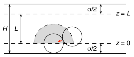
Figure 1: Schematic of hard spheres between planar hard walls. The sphere diameter is denoted by $\sigma$, the surface separation by H, and the reduced slit width by L. The gray region depicts the excluded volume around the left particle, which in this figure is in contact with the bottom wall. The red arrow shows the collisional force exerted by the right particle on the left one. The force acts in the radial direction.

Due to the planar symmetry all pair functions depend on three variables only, e.g., the pair distribution function $g({\bf r}_{1},{\bf r}_{2})=g(z_{1},z_{2},R_{12})$, where $R_{12}=|{\bf R}_{12}|$ with ${\bf R}_{12}=(x_{2}-x_{1},y_{2}-y_{1})$ denotes a distance parallel to the surfaces. In graphical representations of such functions, we let the $z$ axis go through the center of a particle at ${\bf r}_{2}$, i.e., we select ${\bf r}_{2}=(0,0,z_{2})$. Then the function $g(z_{1},z_{2},R_{12})$ states the pair distribution function at position ${\bf r}_{1}=({\bf R}_{12},z_{1})=(x_{1},y_{1},z_{1})$, given a particle at position $(0,0,z_{2})$. Likewise, $n(z_{1})g(z_{1},z_{2},R_{12})$ gives the average density at ${\bf r}_{1}$ around a particle located at $(0,0,z_{2})$. We plot for clarity also negative values of $R_{12}$, i.e., in the following plots of pair functions $R_{12}$ is to be interpreted as a coordinate along a straight line in the $xy$ plane through the origin.

Throughout this study, we make use of integral equation theory for inhomogeneous fluids on the anisotropic pair correlation level. Following Refs. Kjellander and Sarman, 1991a and Kjellander and Sarman, 1988, we determine the density profiles $n(z_{1})$ and pair distribution functions $g(z_{1},z_{2},R_{12})$ of the confined hard-sphere fluid by solving two exact integral equations self-consistently: the Lovett-Mou-Buff-Wertheim equation,

$$\frac{d[{\mathrm{ln}}n(z_{1})+\beta v(z_{1})]}{dz_{1}}=\int c(z_{1},z_{2},R_{12})\frac{dn(z_{2})}{dz_{2}}dz_{2}d{\bf R}_{12},$$ (1)

and the inhomogeneous Ornstein-Zernike equation,

$$h({\bf r}_{1},{\bf r}_{2})=c({\bf r}_{1},{\bf r}_{2})+\int h({\bf r}_{1},{\bf r}_{3})n(z_{3})c({\bf r}_{3},{\bf r}_{2})d{\bf r}_{3},$$ (2)

where $h=g-1$ is the total and $c$ the direct pair correlation function, while $v$ denotes the hard particle-wall potential

$$v(z)=\left\{\begin{array}[]{ll}0&\textrm{if $0\leq z\leq L$,}\\ \infty&\textrm{otherwise.}\end{array}\right.$$ (3)

As the sole approximation, we thereby make use of the Percus-Yevick closure for anisotropic pair correlations, $c=g-y$, where $y({\bf r}_{1},{\bf r}_{2})$ denotes the cavity correlation function that satisfies $g=y\exp(-\beta u)$ and $u$ is the hard particle-particle interaction potential,

$$u({\bf r}_{1},{\bf r}_{2})=\left\{\begin{array}[]{ll}0&\textrm{if $|{\bf r}_{1}-{\bf r}_{2}|\geq\sigma$,}\\ \infty&\textrm{if $|{\bf r}_{1}-{\bf r}_{2}|<\sigma$.}\end{array}\right.$$ (4)

This set of equations constitutes the APY theory.

The confined fluid is kept in equilibrium with a bulk fluid reservoir of a given density by means of a special integration routine, in which the rate of change of the density profile for varying surface separation is given by the exact relationKjellander and Sarman (1991a, 1988)

$$\frac{\partial n(z_{1};L)}{\partial L}=-\beta n(z_{1};L)\bigg{[}\frac{\partial v(z_{1};L)}{\partial L}\\ +\int n(z_{2};L)h(z_{1},z_{2},R_{12};L)\frac{\partial v(z_{2};L)}{\partial L}dz_{2}d{\bf R}_{12}\bigg{]}$$ (5)

under the condition of constant chemical potential. Here we have explicitly shown the $L$ dependence of the functions, which is implicit in the previous equations. For a concise review of the theory and details on the computations we refer to Ref. Nygård, Sarman, and Kjellander, 2013.

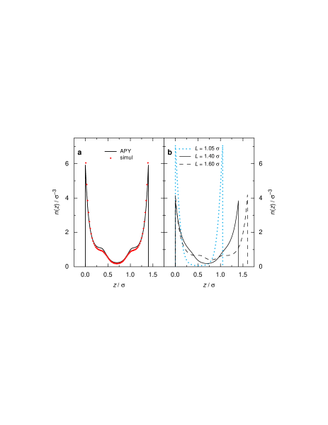
Figure 2: Number density profiles $n(z)$ for the hard-sphere fluid confined between hard planar surfaces. (a) Data for the average volume fraction $\phi_{\mathrm{av}}=0.40$ of particles in the slit of width $H=2.4\sigma$ (reduced slit width $L=1.4\sigma$), which is virtually at phase separation to the crystalline state for this surface separation. The solid line depicts theoretical data within the Anisotropic Percus-Yevick (APY) approximation, while the crosses show data from the Grand-Canonical Monte Carlo simulation of Ref. Mittal, Errington, and Truskett, 2007. (b) Theoretical data from APY approximation for a confined fluid in equilibrium with a bulk reservoir of number density $n_{\mathrm{b}}=0.75\sigma^{-3}$. The reduced slit widths are $L=1.05\sigma$ (dotted line), $1.40\sigma$ (solid line), and $1.60\sigma$ (dashed line). The average volume fraction $\phi_{\mathrm{av}}$ is here 0.35, 0.34, and 0.33, respectively.

III Results and Discussion

III.1 Density profiles and pair densities

The theoretical approach adopted in this work has recently been shownNygård et al. (2012) to be in quantitative agreement with experiments at the pair distribution level for a confined hard-sphere fluid in contact with a bulk fluid of the same density, $n_{\mathrm{b}}=0.75\sigma^{-3}$, as used in the current work. Both the anisotropic structure factors from pair correlations and the density profiles agree very well with the experimental data. For higher densities, we compare in Fig. 2(a) our result with the density profile obtained from GCMC simulations by Mittal et al.Mittal, Errington, and Truskett (2007) for an average volume fraction in the slit $\phi_{\mathrm{av}}=0.40$ and at $L=1.40\sigma$. For this extreme particle density, which is virtually at phase separation to the crystalline phase at this surface separation,Fortini and Dijkstra (2006) there are quantitative differences, but our theoretical profile agree semi-quantitatively with the simulation data. For $L=1.0\sigma$ and $2.0\sigma$ and at the same $\phi_{\mathrm{av}}$, the deviations between our profiles and the GCMC profiles by Mittal et al. are larger (not shown). In the rest of this paper we shall, however, treat cases with lower particle concentrations in the slit: $\phi_{\mathrm{av}}$ between about 0.33 and 0.37, which are less demanding theoretically. In Ref. Kjellander and Sarman, 1988 we showed, for a wide range of slit widths, that our theory is in very good agreement with GCMC simulations for the confined hard sphere fluid in equilibrium with a bulk density $0.68\sigma^{-3}$, which is only slightly lower than what we consider in this work. Furthermore, our main concern in this paper are cases with surface separations about halfway between integer multiples of sphere diameters, as in Fig. 2(a).

Returning to the system in equilibrium with a bulk with density $n_{\mathrm{b}}=0.75\sigma^{-3}$, we illustrate the concept of packing frustration in spatially confined fluids by presenting the number density profile $n(z)$ for reduced slit widths of $L=1.05\sigma$, $1.40\sigma$, and $1.60\sigma$ in Fig. 2(b). The fluid in the narrowest slit exhibits strong ordering, as illustrated by well-developed particle layers close to each solid surface. Such ordering is observed for the hard-sphere fluid in narrow hard slits when the surface separation is close to an integer multiple of the particle diameter $\sigma$. In this specific case, the average volume fraction $\phi_{\mathrm{av}}=0.35$ is about $82\%$ of the volume fraction for phase separation to the crystalline phase at this surface separation,Fortini and Dijkstra (2006) and the “areal” number density near each solid surface is $\int_{0}^{L/2}n(z)dz\approx 0.69\sigma^{-2}$, about $77\%$ of the freezing density for the two-dimensional hard-sphere fluid.Schmidt and Löwen (1996); Fortini and Dijkstra (2006)

For slit widths intermediate between integer multiples of $\sigma$, the confined fluid develops into a relatively disordered fluid in the slit center, despite the confining slit being narrow enough to support ordering across the slit. In the particular case shown in Fig. 2(b), we observe shoulders in the density peaks close to each surface which evolve with increasing slit width into two small (or secondary) density peaks in the slit center. At slightly larger slit widths (to be investigated below), these two small peaks merge and form a fairly broad layer in the middle of the slit. For $L\approx 2.0\sigma$ there is strong ordering again; the layers at either wall are then very sharp and the mid-layer is quite sharp (more profiles for $L=1.0\sigma-4.0\sigma$ for the current case can be found in Ref. Nygård, Sarman, and Kjellander, 2013 and as a video in Ref. not, ). Such a change of ordering at the intermediate separations is usually interpreted as a signature of packing frustration, and in this paper we will address its mechanisms.

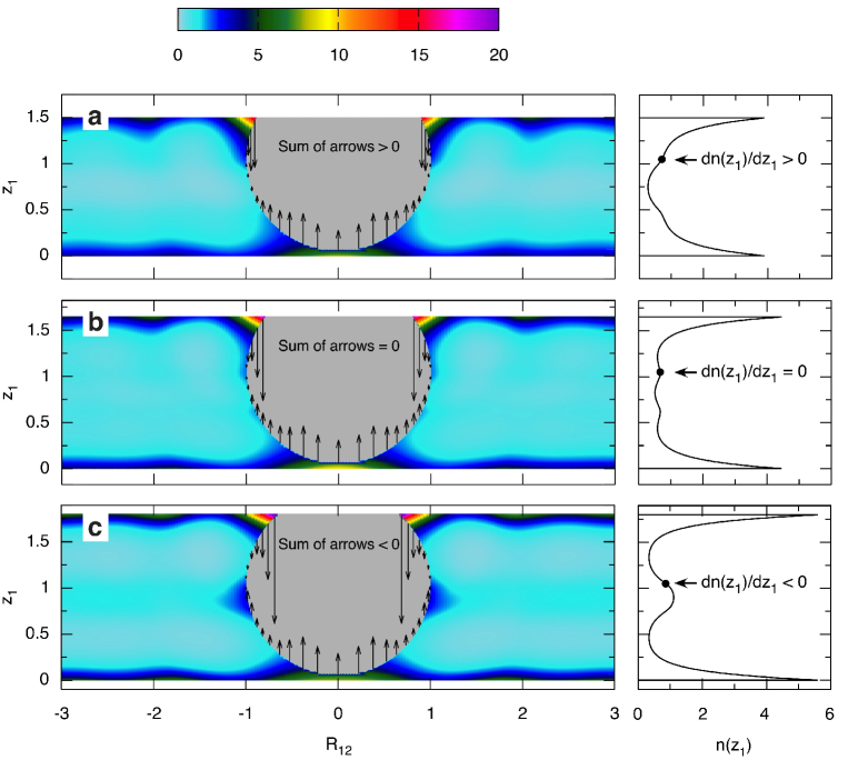
Figure 3: Contour plot of the pair density $n({\bf r}_{1})g({\bf r}_{1},{\bf r}_{2})\equiv n(z_{1})g(z_{1},z_{2},R_{12})$ at coordinate ${\bf r}_{1}=({\bf R}_{12},z_{1})$ around a particle in the slit between two hard surfaces, when the particle is located on the $z$ axis at coordinate ${\bf r}_{2}=(0,0,z_{2})$. One surface is $0.5\sigma$ above the top and one $0.5\sigma$ below the bottom of each subplot (cf. Fig. 1). The system is in equilibrium with a bulk fluid of density $n_{\mathrm{b}}=0.75\sigma^{-3}$ [same as in Fig. 2(b)]. The gray region is the excluded volume zone around the particle. Data are shown for different reduced slit widths: (a) $L=1.50\sigma$, (b) $1.65\sigma$, and (c) $1.80\sigma$. The number density profile $n(z_{1})$ for each case is also shown for clarity to the right. The particle position $z_{2}$ (shown as filled circle in the profile plots) is in all cases positioned at a distance of $1.55\sigma$ from the bottom surface (at $z$ coordinate $1.05\sigma$). The arrows in the gray region depict $z$ components of the collisional forces acting on the particle (corresponding to the $z$ projection of the red arrow in Fig. 1). The arrows displayed at a certain $z_{1}$ coordinate here represent the entire force acting on the sphere periphery in a $dz$ interval around this coordinate. In subplot (a) the sum of all arrows (with signs) is $>0$, in (b) $=0$ and in (c) $<0$.

How can we understand these observations? The starting point for our discussion will be the pair density $n({\bf r}_{1})g({\bf r}_{1},{\bf r}_{2})$, i.e., the density at position ${\bf r}_{1}$ given a particle at position ${\bf r}_{2}$. As will become evident below, the pair densities allow us to analyze the mechanisms leading to the detailed structure of the layers in confined, inhomogeneous fluids. Here, we shall in particular investigate the mechanisms of packing frustration in dense hard-sphere fluids under spatial confinement.

Fig. 3 shows examples of contour plots of the pair density $n(z_{1})g(z_{1},z_{2},R_{12})$ for three reduced slit widths, $L=1.50\sigma$, $1.65\sigma$, and $1.80\sigma$, when a particle (the “central” particle) is located on the $z$ axis at coordinate ${\bf r}_{2}=(0,0,z_{2})$. The density profiles for these three slit widths are shown in the right hand side of the plot. In Fig. 3(a) there is a shoulder in the profile on either side of the midplane, while in Fig. 3(b) two small, but distinct, peaks have formed near the slit center. In Fig. 3(c) these secondary peaks have merged into one peak in the middle. These changes in the density profile occur within a variation in surface separation of only $0.3\sigma$. In the contour plots, the central particle’s center is in all cases situated at a distance of $1.55\sigma$ (about three particle radii) from the bottom surface, $z_{2}=1.05\sigma$, marked by a filled circle in the profile. Particles that form the main layer in contact with the bottom surface can then touch the central particle; the latter is penetrating just the edge of this layer. Note that the position of the secondary maximum for the middle case, Fig. 3(b), is also located at $z_{1}=1.05\sigma$.

Thus, it can be understood that particles forming the small secondary peak in Fig. 3(b) are in contact with, but barely penetrating, the main layer of particles at the bottom surface. The particles of this secondary peak are at the same time strongly penetrating the main layer at the top surface. The same is, however, true for the particles around the same $z$ coordinate ($1.05\sigma$) in Figs. 3(a) and 3(c), but with a markedly different outcome for the profile. Our task here is to understand the reason for such differences.

In the contour plots of the pair density $n(z_{1})g(z_{1},z_{2},R_{12})$ in Fig. 3 we see that in all three cases the particle density in the wedge-like section formed between the central particle and the upper wall is strongly enhanced, resulting in a local number density of up to 17, 20, and 24 $\sigma^{-3}$, respectively, in the three cases. This enhancement in $ng$ relative to the density $n$ at the same $z$ coordinate is given by the pair distribution function $g$, which is about 4 – 4.5 in the inner part of the wedge-like section for all these cases. In the region near the bottom surface, where the central particle is in contact with the main bottom layer, there is also an enhancement in density, but to much smaller extent than at the top. Note that the density distribution $ng$ near the bottom is very similar in all three cases.

III.2 Mean force

To understand why the profiles differ so much in these three cases, we investigate the mean force $F(z)$ that acts on a particle with its center at position $z$. The potential of mean force, $w$, is related to the density $n$ by $n=n_{\mathrm{b}}\exp(-\beta w)$, where $\beta=(k_{B}T)^{-1}$, $k_{B}$ is Boltzmann’s constant, and $T$ the absolute temperature. This implies that $F\equiv-\nabla w=k_{B}T\nabla\ln n$. Due to the planar symmetry, $n$ depends on $z$ only and the total force components in the $x$ and $y$ directions are zero. The mean force $F$ is then directed parallel to the $z$ axis and we have $\beta F(z)=d\ln n(z)/dz=n^{\prime}(z)/n(z)$, where $n^{\prime}=dn/dz$. Thus, an understanding of the behavior of the profile can be obtained from an analysis of $F$. The sign of $F$ tells whether $n$ is increasing or decreasing and extremal points of $n$ correspond to points where $F$ is zero.

For hard-sphere fluids, the forces exerted on a particle by the other particles in the system are simply due to collisions. Due to planar symmetry, the density distribution in the vicinity of a particle has rotational symmetry around the $z$ axis through the particle center. The average force at each point is acting in the direction normal to the sphere surface and for a particle located at $z_{2}$ the average force from all collisions along the sphere periphery at coordinate $z_{1}$ is proportional to the contact density $n(z_{1})g_{\mathrm{cont}}(z_{1},z_{2})$, where $g_{\mathrm{cont}}(z_{1},z_{2})\equiv g(z_{1},z_{2},R_{12})|_{R_{12}^{2}=\sigma^{2}-(z_{1}-z_{2})^{2}}$ is the contact value of the pair distribution function at the particle surface. Note that the force in, for example, the $x$ direction on one side of the periphery is cancelled by the force in the $-x$ direction on the opposite side. Thus only the $z$ component of the net force on the particle contributes as expected. Using the first Born-Green-Yvon equation one can show Kjellander and Sarman (1991a) that

$$\beta F(z_{2})=2\pi\sigma\int^{z_{2}+\sigma}_{z_{2}-\sigma}n(z_{1})g_{\mathrm{cont}}(z_{1},z_{2})\frac{(z_{2}-z_{1})}{\sigma}dz_{1}$$ (6)

(the integral is over the range $|z_{2}-z_{1}|\leq\sigma$ where $g_{\mathrm{cont}}$ is defined). The role of the factor $(z_{2}-z_{1})/\sigma$ is to project out the $z$ component of the contact force. (This line of reasoning is readily extended to systems exhibiting soft interaction potentials, such as Lennard-Jones fluids or electrolytes; in such cases, however, one also needs to include the interactions with the walls and all other particles in the system, see e.g. Refs. Kjellander and Sarman, 1991b and Kjellander, 2009.)

Let us now return to the intriguing formation of secondary density maxima for $L\approx 1.65\sigma$. For this purpose, we present in Fig. 3 the $z$ component of the contact forces acting on the particle. They are represented by the arrows along the sphere periphery. In these plots, there are two major contributions to the net force acting on the particle, namely the repulsive forces exerted by the particle layers close to each confining wall. For $L=1.65\sigma$ and the chosen position of the central particle in Fig. 3(b), $z_{2}=1.05\sigma$, these force contributions cancel each other: the sum of the arrows (with signs) is zero and hence $dn/dz=0$ at this $z$ coordinate, as shown to the right in the figure. It is the subtle interplay between these forces for neighboring $z_{2}$ values which leads to the secondary density maximum.

The situation is, however, markedly different for $L=1.50\sigma$ and $1.80\sigma$. While the total force exerted by the particles in the main layer at the bottom surface is practically equal for all three cases, the magnitude of the force exerted by the particles in the main layer at the upper surface varies strongly with $L$. This variation is partly due to the different magnitude of the contact densities in the wedge-like region mentioned above and partly due to the change in angle between the normal vector to the sphere surface there and the $z$ axis. Recall that the contact force acts along this normal vector, so the $z$ component is dependent on this angle. For $L=1.50\sigma$, Fig. 3(a), the $z$ component of the contact force from the upper layer is smaller than for $L=1.65\sigma$. The sum of the arrows is then positive, i.e. the total average force is directed towards the upper wall and hence $dn/dz>0$ at this $z$ coordinate. For $L=1.80\sigma$, Fig. 3(c), this $z$ component is larger compared to $L=1.65\sigma$, thereby pushing the central particle towards the slit center. Hence $dn/dz<0$ at this $z$ coordinate.

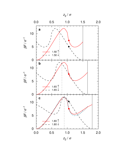
Figure 4: Net forces acting on a particle for the systems in Fig. 3. The force contributions acting in positive ($F_{\uparrow}$, full curve) and negative ($F_{\downarrow}$, dashed curve) $z$ directions are presented separately as functions of particle position $z_{2}$ across the confining slit. Data are shown for reduced slit widths $L=1.50\sigma$, $1.65\sigma$, and $1.80\sigma$. The values of the forces for a particle at the $z_{2}$ coordinates in Fig. 3 are shown by filled circles. The dashed vertical line denotes the slit center, while the solid vertical line on the right-hand side indicates the upper limit for possible $z_{2}$ coordinates of the particle in the slit. For comparison of all three cases, $F_{\uparrow}$ is also shown for $L=1.50\sigma$ (blue dots) and $1.65\sigma$ (black dots) in the bottom panel.

III.3 Principal components of mean force

In order to gain more insight into the formation of the secondary maxima, we present in Fig. 4 the net force acting on a particle for all positions $z_{2}$ in the same three cases as discussed above, $L=1.50\sigma$, $1.65\sigma$, and $1.80\sigma$. To facilitate the interpretation, the principal force contributions acting in positive (denoted $F_{\uparrow}$) and negative ($F_{\downarrow}$) directions are shown separately. The total net force is $F=F_{\uparrow}-F_{\downarrow}$, where $F_{\uparrow}$ originates from collisions on the lower half of the sphere surface and $F_{\downarrow}$ on the upper half ($F_{\uparrow}$ and $F_{\downarrow}$ correspond to the absolute values of the sums of arrows in respective hemisphere in Fig. 3). In Fig. 4 the red (solid) and black (dashed) curves are each other’s mirror images with respect to the vertical dashed axis at $z_{2}=L/2$, which shows the location of the slit center.

Since the variation in $F_{\uparrow}$ (and $F_{\downarrow}$) is very similar for all slit widths in Fig. 4, the following discussion will hold for all three cases. For $z_{2}=0$ we have $F_{\uparrow}=0$, because no spheres can collide from below since the confining surface precludes them from being there (cf. Fig. 1). With increasing $z_{2}$ we observe a monotonically increasing $F_{\uparrow}$, which can be attributed both to the increasing area exposed to collisions on the lower half of the sphere surface and the decrease in angle of the sphere normal there relative to the $z$ axis. With further increase in $z_{2}$, we eventually observe a decrease in the exerted force induced by a decrease in contact density $n(z_{1})g_{\mathrm{cont}}(z_{1},z_{2})$. Around $z_{2}\approx 1.0\sigma$ we observe a sudden onset of a rapid decrease for $F_{\uparrow}$. This is a consequence of a rapid decrease in contact density, that occurs when the particle at $z_{2}$ loses contact with the dense particle layer at the bottom wall. For even larger $z_{2}$, where the particle is close to the top surface, collisions with particles in the slit center around the entire lower half of the sphere surface become important so that $F_{\uparrow}$ increases again.

The three red curves are compared in the bottom panel, where $F_{\uparrow}$ from the first two panels ($L=1.50\sigma$ and $1.65\sigma$) are shown as dotted curves. We see that the curves are nearly identical apart from in a small region to the far right. The analogous statement is true, of course, for the black dashed curves. Thus, apart from small $z_{2}$ intervals to the extreme left and right, the behavior of $F=F_{\uparrow}-F_{\downarrow}$ for the different slit widths can be understood in terms of a horizontal shift of the red and the black curves relative to each other. The formation of secondary density maxima can then be explained from the resulting balance of the force contributions. For $L=1.65\sigma$ and $z_{2}>L/2$ [i.e., the right half of Fig. 4(b)], the two curves intersect at two points where the forces cancel each other and where $dn/dz=0$. The intersection marked by the filled circle gives a local maximum of $n(z)$ and the next one to the right gives a minimum. Together with the minimum at the slit center, $z_{2}=L/2$, where the curves also cross each other, these features give rise to the secondary peak of the density profile as we have seen in Fig. 3(b). This subtle balance of forces, and hence the formation of secondary maxima, is only observed in a narrow range of slit widths, as evidenced by the force profiles for $L=1.50\sigma$ and $1.80\sigma$. In the latter case, the intersection at $z_{2}=L/2$ corresponds to a local maximum and the other one to a minimum. Together they give one peak in the middle as seen in Fig. 3(c).

The formation of secondary maxima is for $z_{2}>L/2$ accordingly a consequence of two phenomena: (i) the rapid decrease of $F_{\uparrow}$ followed by the subsequent increase of $F_{\uparrow}$ and (ii) the monotonic decrease of $F_{\downarrow}$ in the same region. Together these effects lead to the force curves intersecting twice in the manner they do for $L=1.65\sigma$. The rapid decrease of $F_{\uparrow}$ is, as we have seen, due to the loss of contact of the particle with the well-developed bottom layer, while the monotonic decrease of $F_{\downarrow}$ occurs when the particle approaches the top surface.

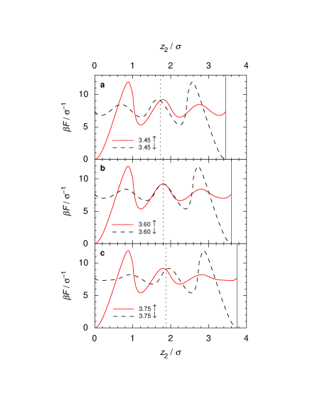
Figure 5: As Fig. 4, but for reduced slit widths $L=3.45\sigma$, $3.60\sigma$, and $3.75\sigma$.

For comparison, we present in Fig. 5 the principal force components for a set of larger slit widths: $L=3.45\sigma$, $3.60\sigma$, and $3.75\sigma$. There are no secondary maxima in this case. Instead we observe for $L=3.60\sigma$ a broad region in the center of the slit where $F_{\uparrow}$ and $F_{\downarrow}$ virtually cancel each other and where, as a consequence, $dn/dz\approx 0$. Hence, this observation implies an essentially constant $n$ in the slit center, as can be seen in the third full curve of Fig. 6, where density profiles are shown for various cases.

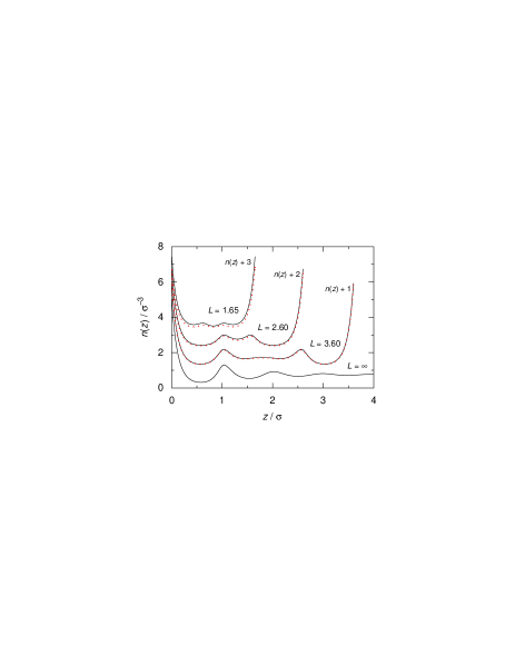
Figure 6: Number density profiles $n(z)$ for the confined hard-sphere fluid. The reduced slit widths are $L=1.65\sigma$ (offset vertically by 3.0$\sigma^{-3}$), $2.60\sigma$ (offset by 2.0$\sigma^{-3}$), and $3.60\sigma$ (offset by 1.0$\sigma^{-3}$). The systems are otherwise the same as in Fig. 2(b). The solid and dotted lines depict results based on the full APY theory and the superposition approximation, respectively. The density profile at a single solid-fluid interface ($L=\infty$) is also shown for comparison.

The course of events shown in Fig. 5 when we increase $L$ from $3.45\sigma$ to $3.75\sigma$ implies the formation of a layer at the slit center. The crossing of the principal force curves in Fig. 5(a) at the slit center, $z_{2}=L/2$, corresponds to a density minimum, while that in Fig. 5(c) corresponds to a density maximum. Note that for $L\approx 3.0\sigma$ there are four layers in the slit (two very sharp ones at the walls and two less sharp on either side of the slit center) and for $L\approx 4.0\sigma$ there are five layers. The fifth layer that forms in the middle for the intermediate separations arises via the broad flattening of the density profile in the middle, and signals the packing frustration in this case.

The data of Figs. 4 and 5 indicate a qualitative difference in $n(z)$ for $L\approx 1.65\sigma$ and $\approx 3.60\sigma$. In the transition from $2\rightarrow 3$ particle layers, the third layer is formed via the occurrence of secondary layers close to each surface, which merge to form a central layer with increasing $L$. This contrasts the transitions from $4\rightarrow 5$ particle layers just discussed, where the new particle layer forms directly in the slit center. The secondary peaks for $L\approx 1.65\sigma$ are also evident in qualitatively different anisotropic structure factors $S({\bf q})$ for $L=1.60\sigma$ and $3.50\sigma$ presented in our previous work, Ref. Nygård, Sarman, and Kjellander, 2013. $S({\bf q})$ for confined fluids is governed by an ensemble average of the anisotropic pair density correlations $n(z_{1})h(z_{1},z_{2},R_{12})$ (see Ref. not, for more slit widths). In order to address these differences in $n(z)$ with $L$, we will in the following analyze further the principal force component $F_{\uparrow}$.

III.4 Superposition approximation

In both Figs. 4 and 5, the principal force components $F_{\uparrow}$ (and $F_{\downarrow}$) for different $L$ nearly coincide for most $z$ values. In order to investigate this further, we plot $F_{\uparrow}$ for a wider set of slit widths, $L=3.0\sigma-4.0\sigma$, in Fig. 7(a). Indeed, apart from rather small deviations at large $z$, all data fall on a master curve given by $F_{\uparrow}$ for $L=\infty$, i.e., the force component for the single solid-fluid interface [the former curves are also shown separated in Fig. 7(b)]. Although not shown here, we have verified that this observation holds reasonably well for $L\geq 1.0\sigma$, implying the same ordering mechanism irrespective of slit width.

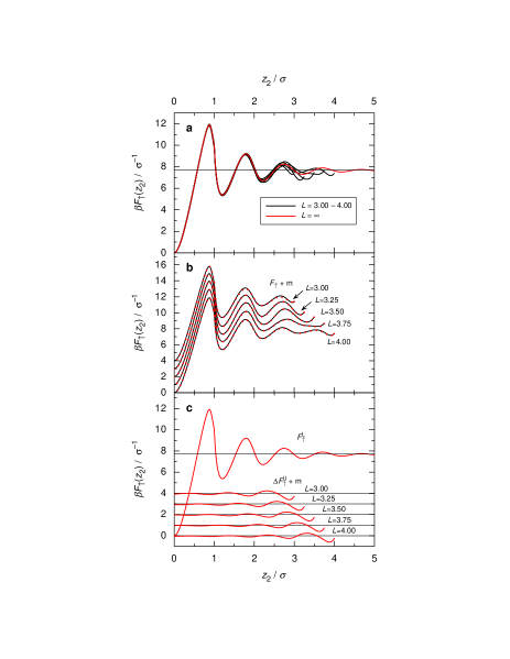
Figure 7: Principal mean force component $F_{\uparrow}$ for the hard-sphere fluid between planar hard surfaces. The reduced separations are $L=3.00\sigma$, $3.25\sigma$, $3.50\sigma$, $3.75\sigma$, and $4.00\sigma$. The systems are otherwise the same as in Fig. 2(b). (a) $F_{\uparrow}$ for the confined fluids (black lines) and for a single solid-fluid interface ($L=\infty$, red line). (b) $F_{\uparrow}$ for the confined fluids (each offset vertically by $m=0...4$ units for clarity), obtained via the full APY theory [solid lines, same as in (a)] and the superposition approximation (dotted lines). (c) Force components of the superposition approximation, $F_{\uparrow}^{\mathrm{L}}$ and $\Delta F_{\uparrow}^{\mathrm{U}}$, for different reduced slit widths (the latter curves are vertically offset by $m$ for clarity). $F_{\uparrow}^{\mathrm{L}}$ is the same as the red curve in (a).

In order to gain further insight into the ordering mechanism, we have determined density profiles obtained in a simple superposition approximation.Percus (1980); Snook and van Megen (1981); Wertheim, Blum, and Bratko (1990); Sarman (1990) Within this approximation, the potential of mean force $w$ in the slit is calculated as the sum of the corresponding potentials from two single hard surfaces, i.e. $w(z)\approx w_{\infty}(z)+w_{\infty}(L-z)$, where $w_{\infty}$ denotes the potential of mean force for the fluid at a single solid-fluid interface in contact with a bulk fluid of density $n_{\mathrm{b}}$. This implies the superposition for the mean force: $F(z)\approx F_{\infty}(z)-F_{\infty}(L-z)$. Since the density profile is given by $n(z)=n_{\mathrm{b}}\exp[-\beta w(z)]$ the superposition approximation implies

$$n(z;L)\approx n^{\mathrm{sp}}(z;L)=\frac{n_{\infty}(z)n_{\infty}(L-z)}{n_{\mathrm{b}}},$$ (7)

where we have explicitly shown that the density profile for the slit, $n(z)\equiv n(z;L)$, depends on $L$, and where superscript sp indicates “superposition” and $n_{\infty}(z)$ is the density profile outside a single surface.

In Fig. 6 we compare $n(z)$ for reduced slit widths of $L=1.65\sigma$, $2.60\sigma$, and $3.60\sigma$ obtained via the full theory (solid lines) and the superposition approximation thus obtained (dotted lines). Note that there are density peaks at $z\approx 1.05\sigma$ for all three slit widths and that they approximately coincide with the location of a density peak for the single solid-fluid interface (also shown in Fig. 6). This implies that the density peak at $z\approx 1.05\sigma$ is strongly correlated with the bottom solid surface. Although the profiles obtained via the superposition approximation deviate quantitatively from those of the full theory, especially for narrow slit widths, the qualitative agreement implies that the main features of $n(z)$ – the density peaks and shoulders of Fig. 6 – are rather uncomplicated confinement effects.

To substantiate this conclusion, we present in Fig. 7(b) the principal force components $F_{\uparrow}$ for $L=3.0\sigma-4.0\sigma$, obtained both using the full theory and the superposition approximation. The agreement is equally good as for the density profile of the $L=3.60\sigma$ case in Fig. 6. A significant point is now that the superposition allows us to separate the contributions to $F_{\uparrow}$ from each surface in a simple manner, that will provide insights into what happens during confinement. As shown in Appendix A, $F_{\uparrow}$ can be decomposed in this approximation into two components: a major contribution from the lower surface, $F_{\uparrow}^{\mathrm{L}}$, and a correction due to the presence of the upper surface, $\Delta F_{\uparrow}^{\mathrm{U}}$. The former is the same as the average force component for the single solid-fluid interface plotted in Fig. 7(a) (denoted as “master curve” above). We have

$$F^{\mathrm{sp}}_{\uparrow}(z_{2};L)=F_{\uparrow}^{\mathrm{L}}(z_{2})+\Delta F_{\uparrow}^{\mathrm{U}}(z_{2};L),$$ (8)

where $\Delta F_{\uparrow}^{\mathrm{U}}(z_{2};L)=F_{\uparrow}^{\mathrm{U}}(z_{2};L)-F_{\uparrow}^{\mathrm{b}}$, see Eq. (16). Here, $F_{\uparrow}^{\mathrm{U}}$ is the average force for the case of a single solid-fluid interface (U) and $F_{\uparrow}^{\mathrm{b}}$ is the force that acts on one side of a hard sphere (i.e. on one half) in the bulk fluid. Note that in $F^{\mathrm{sp}}_{\uparrow}$ it is only $F_{\uparrow}^{\mathrm{U}}$ that depends on $L$.

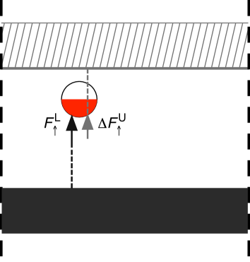
Figure 8: A sketch illustrating the force contributions $F_{\uparrow}^{\mathrm{L}}$ and $\Delta F_{\uparrow}^{\mathrm{U}}$ in the superposition approximation. Each arrow represents a force that acts on the entire red half of the sphere (the location of the arrow has no significance in this sketch). The lower wall is shown in black and the upper wall is to be placed on the location indicated by the striped rectangle. The dashed line that connects each arrow to the respective surface indicates from which wall the influence originates.

In Fig. 7(c) we show $F_{\uparrow}^{\mathrm{L}}$ and $\Delta F_{\uparrow}^{\mathrm{U}}$ for the same surface separations as before. The $L$ dependence of the latter is simply a parallel displacement along $z$. When $F_{\uparrow}^{\mathrm{L}}$ and $\Delta F_{\uparrow}^{\mathrm{U}}$ are added we obtain the dotted curves in Fig. 7(b). Thus the differences between each black curve and the red curve in Fig. 7(a) is essentially contained in the contribution $\Delta F_{\uparrow}^{\mathrm{U}}$ from the upper surface (for smaller surface separations there will remain a minor difference as indicated by the small deviations for the superposition approximation in Fig. 6).

To see in more detail what this means, we have in Fig. 8 shown schematically how these force contributions act on a sphere. In the presence of only one solid-fluid interface (L), the total force in the direction away from the surface (upwards) is $F_{\uparrow}=F_{\uparrow}^{\mathrm{L}}$, i.e., the force on the bottom half of the sphere shown as red in the figure. Let us now place the second surface (U) some distance from the other, at the location indicated in the figure. The change in the upwards force due to this second surface is given by $\Delta F_{\uparrow}\approx\Delta F_{\uparrow}^{\mathrm{U}}$ in the superposition approximation. Note that the former force, $F_{\uparrow}^{\mathrm{L}}$, acts on the hemisphere that is facing the surface L, while the latter, $\Delta F_{\uparrow}^{\mathrm{U}}$, is a force that acts on the hemisphere away from the corresponding surface U and in the direction towards this surface.

If the lower wall were not present when we place the upper wall at the indicated position, the initial state would be a homogeneous bulk fluid and the final state a single solid-fluid interface (U) in contact with the bulk. In this situation $\Delta F_{\uparrow}^{\mathrm{U}}$ equals the actual change in the average force on the red hemisphere. In Eq. (8) we have adopted this value as an approximation for the corresponding change when placing the upper wall in the presence of the lower one, i.e., when the initial state is an inhomogeneous fluid in contact with the lower surface and the final state is a fluid simultaneously affected by both surfaces. Since this approximation obviously is very good, it follows that the inhomogeneity due to one surface has only a small influence on the effects from the other surface throughout the entire slit.

We saw in section III.3 that the seemingly complicated changes in structure as the surface separation varies around half-integer $\sigma$ values of $L$ (i.e., $[m+0.5]\sigma$ with $m=$ integer), can be mainly explained by a parallel displacement of upward and downwards force curves along the $z$ direction. There was, however, some variation in these force curves near one of the surfaces (the upper surface for the upward forces and the lower surface for the downwards forces) that remained unexplained there. In the current section we have seen that this variation too can be mainly explained by a parallel displacement – in this case a displacement of the contributions to $F_{\uparrow}$ (or $F_{\downarrow}$) due to each surface as seen in Fig. 7(c).

To summarize our results in this section we make two important conclusions: First, by considering the mean force due to one surface (here the lower one) and by treating the influence from the other (upper) surface as a correction $\Delta F_{\uparrow}^{\mathrm{U}}$ according the the superposition approximation, one obtains nearly quantitative agreement with the full theory. Our approach of defining principal components of the mean force thereby provides a means to understand the contributions of each confining surface. Second, the principal force components obtained within the full theory and the superposition approximation are virtually in quantitative agreement for $L\geq 3.0\sigma$. For narrower slit widths (down to $L=1.0\sigma$), quantitative discrepancies become more pronounced. These quantitative differences, which will be discussed in the next subsection, are nontrivial confinement effects. Nevertheless, the semi-quantitative agreement in the whole range of slit widths, down to $L=1.0\sigma$, further strengthens the notion that ordering of confined hard-sphere fluids can, to a good approximation, be explained as a single-wall phenomenon. In essence, the fluid conforms locally with only one of the confining surfaces at a time. In some local regions it will thereby conform to one surface and in other regions to the other surface – regions that are continuously changing (recall that the distributions we calculate are time averages of the various possible structures). We emphasize that this reasoning holds for all slit widths, irrespective of whether $L$ is close to an integer or a half-integer multiple of the particle diameter (cf. Fig. 7). In other words, from a mechanistic point of view there is little difference between ordering in frustrated and more ordered confined hard-sphere fluids. In the latter case, the local ordering near one surface essentially agrees with the local ordering at the other one, whereby for the density profiles there appear only small mutual effects of the ordering from both surfaces beyond what is given by superposition.

An interesting similarity between the structures observed in the fluid and solid phases should be mentioned. In some of the exotic crystalline structures observed under confinement – most notably the prism-like structures Neser et al. (1997); Fortini and Dijkstra (2006); Oğuz et al. (2012) – the particles locally conform with one of the solid surfaces. This is reminiscent of the situation in the fluid phase discussed above, although in the latter case the structures are less ordered and constantly changing locally. In particular, the adaptive prism phase $2P_{A}$ found in Ref. Oğuz et al., 2012 would yield an average density profile with secondary peaks on either side of the midplane, similar of those shown in Fig. 3(b) but much sharper.

The fact that the superposition approximation works surprisingly well for these rather large densities and gives a large part of the effects of confinement, means that it is simple to obtain good estimates of the density profiles for a confined fluid given an accurate density profile for a single solid-fluid interface. To obtain the latter is, however, computationally nontrivial and requires fairly advanced theories. Furthermore, as we shall see below, not all important properties of the confined fluid can be explained by superposition.

Figure 9: (a) Excess adsorption $\Gamma$ and (b) contact density $n_{\mathrm{cont}}=n(0)$ of hard spheres between two hard planar surfaces as functions of reduced surface separation. The system is in equilibrium with a bulk fluid of density $n_{\mathrm{b}}=0.75\sigma^{-3}$ [same as in Fig. 2(b)]. Data are shown for both the full APY theory (solid lines) and the superposition approximation (dashed lines).

III.5 Nontrivial confinement effects

We have shown that the density profile $n(z)$ of confined hard-sphere fluids is, to a large extent, determined by packing constraints at a single solid-fluid interface. In this respect, the ordering is a trivial confinement effect. However, subtle deviations in $n(z)$ do remain in the superposition approximation, and these may lead to important, nontrivial confinement effects. The two most prominent nontrivial effects of confinement in, for example, Fig. 6 are the slit width dependence of the contact density at the walls, $n_{\mathrm{cont}}$, and the total number of particles per unit area in the slit $N=\int_{0}^{L}n(z)dz$, which is a fundamental quantity for many properties of the confined fluid. In the following, we will discuss these two and related quantities in more detail.

In Fig. 9(a), we present the excess adsorption $\Gamma(L)=\int_{0}^{L}[n(z)-n_{\mathrm{b}}]dz$ of particles in the slit as a function of reduced slit width $L$, determined via both the full theory and the superposition approximation. The discrepancy between the two theoretical schemes is striking; since $\Gamma$ is an integrated quantity, minor systematic deviations in $n(z)$ accumulate to a large effect in the total number of particles. The superposition approximation gives, for example, in the interval $L=1.0\sigma$ to $2.0\sigma$ an estimate of $N$ that is wrong by a factor that varies between 1.36 and 0.84. We note that, e.g., dynamic quantities such as diffusion coefficientsMittal, Errington, and Truskett (2006) and relaxation timesIngebrigtsen et al. (2013) in simple confined fluids have been found to scale with particle packing, as quantified by the excess entropy. Consequently, a systematic error in the packing of particles (especially for very narrow confinement), as evidenced by systematic quantitative differences in the number density $n(z;L)$ and an ensuing large discrepancy in $\Gamma(L)$ between the full theory and the superposition approximation, will have a substantial impact on many properties of the confined fluid obtained theoretically.

Fig. 9(b) shows the contact density $n_{\mathrm{cont}}=n(0)$ as a function of $L$, again obtained both via the full theory and the superposition approximation. This is an important quantity, because it yields the pressure between the walls, $P_{\mathrm{in}}=k_{\mathrm{B}}Tn(0)$, according to the contact theorem. Consequently, $n_{\mathrm{cont}}$ is related to the net pressure acting on the confining surfaces, $\Pi(L)=P_{\mathrm{in}}(L)-P_{\mathrm{b}}$ with $P_{\mathrm{b}}$ denoting the bulk pressure, and hence to the extensively studied oscillatory surface forces.Horn and Israelachvili (1981); Israelachvili (1991) While the superposition approximation explains reasonably well the magnitude of $n_{\mathrm{cont}}$, there is a nontrivial systematic phase shift with respect to $L$ of about $0.1\sigma$. This effect has been observed by one of us (S.S.) already earlier,Sarman (1990) and in the following we will provide a mechanistic explanation of the phenomenon. A similar phase shift can also be seen in $\Gamma(L)$, Fig. 9(a).

In the superposition approximation, Eq. (7) yields the contact density for the wall at $z=0$ as

$$n^{\mathrm{sp}}_{\mathrm{cont}}(L)=n^{\mathrm{sp}}(0;L)=\frac{n_{\infty}(0)n_{\infty}(L)}{n_{\mathrm{b}}}.$$ (9)

Thus, the contact density for a reduced slit width $L$ is in this approximation proportional to the density at $z=L$ outside a single surface. To analyze the $L$ dependence further we will need the following equation that is equivalent to Eq. (1),

$$\frac{d[\ln n(z_{1})+\beta v(z_{1})]}{dz_{1}}=\\ -\beta\int n(z_{2})h(z_{1},z_{2},R_{12})\frac{dv(z_{2})}{dz_{2}}dz_{2}d{\bf R}_{12}.$$ (10)

[The two equations can be transformed into each other by the Ornstein-Zernike equation (2).] For a single hard wall-fluid interface located at $z=0$, Eq. (10) yields

$$\frac{dn_{\infty}(z_{1})}{dz_{1}}=n_{\infty}(z_{1})n_{\infty}(0)\int h_{\infty}(z_{1},0,R_{12})d{\bf R}_{12},$$ (11)

where $h_{\infty}$ is the total pair correlation function for the fluid outside the single surface. By inserting $z_{1}=L$, this equation together with Eq. (9) imply that

$$\frac{dn^{\mathrm{sp}}_{\mathrm{cont}}(L)}{dL}=n^{\mathrm{sp}}_{\mathrm{cont}}(L)n_{\infty}(0)\int h_{\infty}(z_{1},0,R_{12})d{\bf R}_{12}\biggl{|}_{z_{1}=L}.$$ (12)

For the exact case, the corresponding equation can be obtained from Eq. (5), which yields

$$\frac{dn_{\mathrm{cont}}(L)}{dL}=[n_{\mathrm{cont}}(L)]^{2}\int h(z_{1},0,R_{12})d{\bf R}_{12}\biggl{|}_{z_{1}=L}.$$ (13)

Apart from the factors in front of the integral, we see that the main difference is that in the superposition approximation the total pair correlation function for a single wall is evaluated at coordinate $z_{1}=L$ outside the wall, while for the exact case the correlation function for the fluid in the slit is evaluated at the opposite surface (also at $z_{1}=L$). The oscillatory behavior of the contact density as a function of $L$ implies that its derivative changes sign with the same periodicity. Since the prefactors are positive, the phase shift for $n^{\mathrm{sp}}_{\mathrm{cont}}$ relative to $n_{\mathrm{cont}}$ must originate from the integrals.

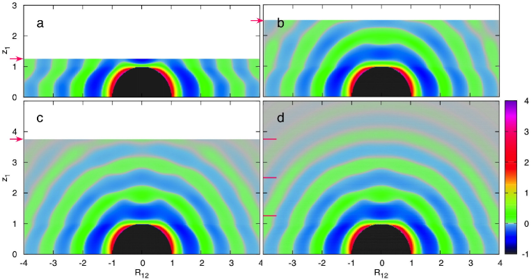
Figure 10: Contour plot of the total pair correlation function $h(z_{1},0,R_{12})$ at coordinate $({\bf R}_{12},z_{1})$ around a particle located on the $z$ axis at coordinate 0, i.e., in contact with the bottom surface. Data are shown for different reduced slit widths: (a) $L=1.25\sigma$, (b) $2.50\sigma$, (c) $3.75\sigma$, and (d) the single solid-fluid interface ($L=\infty$). The systems are otherwise the same as in Fig. 2(b). A small interval around $h=0$ is shown as gray in the contour scale and the black areas denote the core region where $h=-1$. The red horizontal lines on the left hand side in (d) show the $z$ coordinate for spheres in contact with the top surface in subplots (a)$-$(c), i.e., at coordinate $z_{1}=L$ (cf. the red arrow in each of these subplots).

In Fig. 10 we have plotted the total pair correlation function $h(z_{1},0,R_{12})$ in the slit when the central particle is in contact with the lower surface (i.e., at coordinate 0) for the cases $L=1.25\sigma$, $2.50\sigma$, and $3.75\sigma$ together with the corresponding function for a single hard wall-fluid interface. The first impression is a striking similarity of these plots, despite that there is an upper surface present in the first three cases. There are only small differences in the entire slit compared to the single surface case for the corresponding $z_{1}$ values. When looking closely, one can, however, see some systematic differences in the $h$ function induced by the presence of the upper surface. Most importantly, we will investigate $h$ for $z_{1}=L$, which occurs in the integral in Eq. (13), and compare this with the values at the same $z_{1}$ coordinates for the single surface case, occurring in Eq. (12). These $z_{1}$ values are marked with red arrows in the left hand side of Figs. 10(a)–(c) and with red lines in Fig. 10(d).

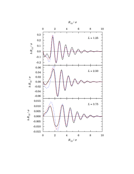
Figure 11: $R_{12}\times h(L,0,R_{12})$ as function of $R_{12}$ for the systems in Fig. 10(a)-(c) with reduced surface separations $L=1.25\sigma$, $L=2.50\sigma$, and $L=3.75\sigma$. The data are obtained via full APY theory (solid line), superposition approximation (blue dotted line), and shifted superposition approximation ($L\rightarrow L+0.1\sigma$, red dotted line). In the latter two cases, $R_{12}\times h_{\infty}(z_{1},0,R_{12})$ is plotted for the appropriate $z_{1}$ values (see text). Note the different scales on the $y$ axis in the subplots. The curves go to zero at $R_{12}=0$ because of the factor $R_{12}$.

Fig. 11 shows $R_{12}\times h(z_{1},0,R_{12})$ with $z_{1}=L$ for the cases in Figs. 10(a)–(c) and these curves are compared to $R_{12}\times h_{\infty}(z_{1},0,R_{12})$ for the same $z_{1}$ coordinates (shown as blue dotted lines in the figure). The factor $R_{12}$ is included so the areas under the curves in Fig. 11 are proportional to the values of the integrals of Eqs. (12) and (13); this factor originates from the area differential $d{\bf R}_{12}=2\pi R_{12}dR_{12}$. The $L$ values in Figs. 10 and 11 are selected such that we cover cases where $dn_{\mathrm{cont}}(L)/dL$ and $dn^{\mathrm{sp}}_{\mathrm{cont}}(L)/dL$ in Fig. 9(b) are negative ($L=1.25\sigma$) and positive ($L=3.75\sigma$). There is also one case ($L=2.50\sigma$) with $dn^{\mathrm{sp}}_{\mathrm{cont}}(L)/dL\approx 0$. These signs can be verified by inspection of the areas under the curves in Fig. 11 (the contributions around $R_{12}=0$ are most important for the sign; there are substantial cancellations in the tail region due to the oscillations).

We can see in the figure that the full curves and the blue dotted ones do not agree, which means that the values of the integrals and hence of $dn_{\mathrm{cont}}(L)/dL$ are different, as expected. If we instead plot the values of $R_{12}\times h_{\infty}(z_{1},0,R_{12})$ for $z_{1}=L+0.1\sigma$ (red dotted lines in the figure) we obtain better agreement. Thus the presence of the upper surface makes $h(z_{1},0,R_{12})$ “compressed” in the $z$ direction by about $0.1\sigma$ compared to $h_{\infty}(z_{1},0,R_{12})$. This compression gives rise to the phase shift observed in Fig. 9. There are also some other small differences between $h$ and $h_{\infty}$ and, in addition, there are different prefactors in Eqs. (12) and (13). This gives the remaining differences in $n_{\mathrm{cont}}(L)$ and $n^{\mathrm{sp}}_{\mathrm{cont}}(L)$ seen in Fig. 9(b).

The nontrivial confinement effects are accordingly due to rather delicate changes in the pair distribution function $g(z_{1},z_{2},R_{12})$ due to the presence of a second solid surface. The packing of particles in the slit around each individual particle is described by the pair density $n(z_{1})g(z_{1},z_{2},R_{12})$ and the changes in $ng$ can be large, even for small variations in $g$, in regions where the density profile $n$ is large. Conversely, since there are large variations in the density profiles with surface separation, the packing is strongly altered even when the change in $g$ is small.

IV Summary and conclusions

The self-consistent calculation of density profiles and anisotropic pair distribution functions, as provided by integral equation theories at the pair correlation level (like the APY theory used in this paper), gives efficient tools for the investigation of the structure of inhomogeneous fluids in confinement. This is exemplified in this paper by a detailed examination of the mechanism behind the packing frustration for a dense hard-sphere fluid confined between planar hard walls at short separations.

When the width of the slit between the walls is close to an integer multiple of sphere diameters, the layer structure is optimal and the number density profile $n(z)$ between the walls has sharp peaks. For slit widths near half-integer multiples of sphere diameters ($[m+0.5]\sigma$ with $m=$ integer), the layer structure is much weaker and the packing frustration is large. The density profile shows considerable intricacy when the slit width is varied around these latter values. For example, when the reduced slit width $L$ is increased from $1.0\sigma$, there appear secondary density peaks close to the main peaks at each wall. These secondary peaks merge into a single peak at the slit center when $L$ approaches $2.0\sigma$. The mechanism behind these and other structural changes have been investigated in this paper, using the tools provided by the anisotropic pair distribution function theory.

The number density profile is determined by the mean force $F(z)$ on the particles in the slit via the relationship $d\ln n(z)/dz=\beta F(z)$. For the hard-sphere fluid the mean force, which acts on a particle located at $z$, originates from collisions by other particles at the surface of the former. The average collisional force on the sphere periphery is proportional to the contact density there, which varies around the surface since the fluid is inhomogeneous. The sum of the average collisional forces constitutes the mean force $F$ and since we have access to the pair distribution, and thereby the contact density at the sphere surface, we can investigate the origin of any variations in $F$ and thereby in $n$. Of particular interest here are the variations when the slit width is changed.

By introducing the two principal components $F_{\uparrow}$ and $F_{\downarrow}$ of $F$, each of which is the sum of the average collisional forces on the particle hemisphere facing one of the walls, we extract sufficient information from the pair distributions to obtain a lucid description of the causes for the structural changes due to varying degree of packing frustration. We show that most features of the structural changes, including the appearance and merging of the secondary peaks mentioned above, can be explained by a simple parallel displacement of the $F_{\uparrow}$ and $F_{\downarrow}$ curves when the slit width is varied around half-integer $\sigma$ values. The underlying reasons for this simple behavior is revealed via a detailed investigation of the pair distribution, that gives information about how the contact densities around the sphere periphery varies for different positions $z$ of a particle in the slit.

It is found that the components $F_{\uparrow}$ and $F_{\downarrow}$, and thereby the ordering of the fluid, are essentially governed by the packing conditions at each single solid-fluid interface. The fluid in the slit thereby conforms locally with only one of the confining surfaces at a time. In some local regions it will conform to one surface and in other regions to the other surface – regions that are constantly changing (the calculated distributions are averages of the various possible structures). This picture holds for all slit widths, irrespective of whether $L$ is close to an integer or a half-integer multiple of the particle diameter.

As a consequence of these local packing conditions, the force components $F_{\uparrow}$ and $F_{\downarrow}$, and thereby the total mean force $F=F_{\uparrow}-F_{\downarrow}$ acting on a particle in the slit, can to a surprisingly good approximation be written as a superposition of contributions due to the presence of each individual solid-fluid interface at the walls. When the slit width is varied, this superposition can be expressed in terms of a parallel displacement of force curves due to either surface.

There are, however, some important properties of the inhomogeneous fluid that cannot be described by a simple superposition, but are instead determined by nontrivial confinement effects. In this paper, we exemplify such quantities by the number of particles per unit area in the slit $N$, the excess adsorption $\Gamma$, the contact density of the fluid at the wall surfaces $n(0)$, and the net interaction pressure between the walls $\Pi$. In the superposition approximation, $N$ and $\Gamma$ disagree to a large extent compared to the accurate values, while $n(0)$ and $\Pi$ are mainly off by a phase shift in their oscillations. The analysis show that these nontrivial confinement effects are due to rather delicate changes in the anisotropic pair distribution function $g(z_{1},z_{2},R_{12})$ when the wall separation is changed.

Appendix A Force subdivision in superposition approximation

For a hard sphere fluid in the slit between two hard walls, the force on, for example, the lower hemisphere of a hard sphere, $F_{\uparrow}$, can in the superposition approximation be divided into contributions due to either wall surface. The contribution $F_{\uparrow}^{\mathrm{L}}$ from the lower surface is given by [cf. Eq. (6)]

$$\beta F_{\uparrow}^{\mathrm{L}}(z_{2})=2\pi\int^{z_{2}}_{z_{2}-\sigma}dz_{1}n_{\infty}(z_{1})g^{\mathrm{cont}}_{\infty}(z_{1},z_{2})(z_{2}-z_{1}),$$ (14)

where $g^{\mathrm{cont}}_{\infty}$ is the contact value of the pair distribution for the fluid outside a single surface. Likewise, the contribution $F_{\uparrow}^{\mathrm{U}}$ from the upper surface is given by

$$\beta F_{\uparrow}^{\mathrm{U}}(z_{2};L)=2\pi\int^{z_{2}}_{z_{2}-\sigma}dz_{1}n_{\infty}(L-z_{1})\\ \times g^{\mathrm{cont}}_{\infty}(L-z_{1},L-z_{2})(z_{2}-z_{1}).$$ (15)

In the total $F^{\mathrm{sp}}_{\uparrow}$ there is a further contribution. From Eq. (7) we see that the total $\beta F^{\mathrm{sp}}$ is equal to the derivative of $\ln n^{\mathrm{sp}}(z;L)=\ln n_{\infty}(z)+\ln n_{\infty}(L-z)-\ln n_{\mathrm{b}}$. While the last term gives zero for $\beta F^{\mathrm{sp}}$, i.e., the mean force in bulk is zero, this is not the case for $\beta F^{\mathrm{sp}}_{\uparrow}$. The mean force on one half of the sphere surface in bulk, $F_{\uparrow}^{\mathrm{b}}$, is non-zero; it is only the sum of the forces on both halves that are zero. Thus we have

$$F^{\mathrm{sp}}_{\uparrow}(z_{2};L)=F_{\uparrow}^{\mathrm{L}}(z_{2})+F_{\uparrow}^{\mathrm{U}}(z_{2};L)-F_{\uparrow}^{\mathrm{b}}$$ (16)

with $\beta F_{\uparrow}^{\mathrm{b}}=\pi\sigma^{2}n_{\mathrm{b}}g^{\mathrm{cont}}_{\mathrm{b}}$, where $g^{\mathrm{cont}}_{\mathrm{b}}$ is the contact value for the pair distribution in bulk. When $L\rightarrow\infty$, the presence of the last term makes $F^{\mathrm{sp}}_{\uparrow}$ go to the single surface force $F_{\uparrow}^{\mathrm{L}}$, as it should in this limit.

References

- Pieranski, Strzelecki, and Pansu (1983) P. Pieranski, L. Strzelecki, and B. Pansu, Phys. Rev. Lett. 50, 900 (1983).
- Schmidt and Löwen (1996) M. Schmidt and H. Löwen, Phys. Rev. Lett. 76, 4552 (1996).
- Neser et al. (1997) S. Neser, C. Bechinger, P. Leiderer, and T. Palberg, Phys. Rev. Lett. 79, 2348 (1997).
- Fortini and Dijkstra (2006) A. Fortini and M. Dijkstra, J. Phys.: Condens. Matter 18, L371 (2006).
- Fontecha and Schöpe (2008) A. B. Fontecha and H. J. Schöpe, Phys. Rev. E 77, 061401 (2008).
- Oğuz et al. (2012) E. C. Oğuz, M. Marechal, F. Ramiro-Manzano, I. Rodriguez, R. Messina, F. J. Meseguer, and H. Löwen, Phys. Rev. Lett. 109, 218301 (2012).
- Pusey and van Megen (1986) P. N. Pusey and W. van Megen, Nature 320, 340 (1986).
- Nygård, Sarman, and Kjellander (2013) K. Nygård, S. Sarman, and R. Kjellander, J. Chem. Phys. 139, 164701 (2013).
- Mittal, Errington, and Truskett (2007) J. Mittal, J. R. Errington, and T. M. Truskett, J. Chem. Phys. 126, 244708 (2007).
- Mittal et al. (2008) J. Mittal, T. M. Truskett, J. R. Errington, and G. Hummer, Phys. Rev. Lett. 100, 145901 (2008).
- Lang et al. (2010) S. Lang, V. Boţan, M. Oettel, D. Hajnal, T. Franosch, and R. Schilling, Phys. Rev. Lett. 105, 125701 (2010).
- Lang et al. (2012) S. Lang, R. Schilling, V. Krakoviack, and T. Franosch, Phys. Rev. E 86, 021502 (2012).
- Hansen and McDonald (2006) J.-P. Hansen and I. R. McDonald, Theory of Simple Liquids, 3rd ed. (Academic Press, Amsterdam, 2006).
- Kjellander and Marčelja (1988) R. Kjellander and S. Marčelja, J. Chem. Phys. 88, 7138 (1988).
- Kjellander and Sarman (1991a) R. Kjellander and S. Sarman, J. Chem. Soc. Faraday Trans. 87, 1869 (1991a).
- Kjellander and Sarman (1991b) R. Kjellander and S. Sarman, Mol. Phys. 74, 665 (1991b).
- Götzelmann and Dietrich (1997) B. Götzelmann and S. Dietrich, Phys. Rev. E 55, 2993 (1997).
- Boţan et al. (2009) V. Boţan, F. Pesth, T. Schilling, and M. Oettel, Phys. Rev. E 79, 061402 (2009).
- Henderson, Sokolowski, and Wasan (1997) D. Henderson, S. Sokolowski, and D. Wasan, J. Stat. Phys. 89, 233 (1997).
- Zwanikken and Olvera de la Cruz (2013) J. W. Zwanikken and M. Olvera de la Cruz, Proc. Natl. Acad. Sci. USA 110, 5301 (2013).
- Kjellander and Sarman (1988) R. Kjellander and S. Sarman, Chem. Phys. Lett. 149, 102 (1988).
- Greberg, Kjellander, and Åkesson (1997) H. Greberg, R. Kjellander, and T. Åkesson, Molec. Phys. 92, 35 (1997).
- Roth (2010) R. Roth, J. Phys.: Condens. Matter 22, 063102 (2010).
- Nygård et al. (2012) K. Nygård, R. Kjellander, S. Sarman, S. Chodankar, E. Perret, J. Buitenhuis, and J. F. van der Veen, Phys. Rev. Lett. 108, 037802 (2012).
- (25) For videos of the density profile as a function of slit width, see the Supplementary material of Ref. Nygård, Sarman, and Kjellander, 2013, Video 2, at ftp://ftp.aip.org/epaps/journ_chem_phys/E-JCPSA6-139-037340. Videos of pair distributions and anisotropic structure factors for the system can also be found there.
- Kjellander (2009) R. Kjellander, J. Phys.: Condens. Matter 21, 424101 (2009).
- Percus (1980) J. K. Percus, J. Stat. Phys. 23, 657 (1980).
- Snook and van Megen (1981) I. K. Snook and W. van Megen, J. Chem. Soc. Faraday Trans. 2 77, 181 (1981).
- Wertheim, Blum, and Bratko (1990) M. S. Wertheim, L. Blum, and D. Bratko, in Micellar Solutions and Microemulsions, edited by S.-H. Chen and R. Rajagopalan (Springer-Verlag, New York, 1990) p. 99.
- Sarman (1990) S. Sarman, in Liquids at Interfaces, edited by J. Charvolin, J. F. Joanny, and J. Zinn-Justin (Elsevier, Amsterdam, 1990) p. 169.
- Mittal, Errington, and Truskett (2006) J. Mittal, J. R. Errington, and T. M. Truskett, Phys. Rev. Lett. 96, 177804 (2006).
- Ingebrigtsen et al. (2013) T. S. Ingebrigtsen, J. R. Errington, T. M. Truskett, and J. C. Dyre, Phys. Rev. Lett. 111, 235901 (2013).
- Horn and Israelachvili (1981) R. G. Horn and J. N. Israelachvili, J. Chem. Phys. 75, 1400 (1981).
- Israelachvili (1991) J. N. Israelachvili, Intermolecular and Surface Forces, 2nd ed. (Academic Press, London, 1991).