Lovelock black holes with nonmaximally symmetric horizons

Abstract

We present a new class of black hole solutions in third-order Lovelock gravity whose horizons are Einstein space with two supplementary conditions on their Weyl tensors. These solutions are obtained with the advantage of higher curvature terms appearing in Lovelock gravity. We find that while the solution of third-order Lovelock gravity with constant-curvature horizon in the absence of a mass parameter is the anti de Sitter (AdS) metric, this kind of solution with nonconstant-curvature horizon is only asymptotically AdS and may have horizon. We also find that one may have an extreme black hole with non-constant curvature horizon whose Ricci scalar is zero or a positive constant, while there is no such black hole with constant-curvature horizon. Furthermore, the thermodynamics of the black holes in the two cases of constant- and nonconstant-curvature horizons are different drastically. Specially, we consider the thermodynamics of black holes with vanishing Ricci scalar and find that in contrast to the case of black holes of Lovelock gravity with constant-curvature horizon, the area law of entropy is not satisfied. Finally, we investigate the stability of these black holes both locally and globally and find that while the black holes with constant curvature horizons are stable both locally and globally, those with nonconstant-curvature horizons have unstable phases.

I Introduction

Higher-order curvature theories of gravity have gained a lot of attention. Not surprisingly, the mere extension of general relativity in higher dimensions can immediately lead to a wide variety of alternative theories of gravity whose actions contain higher-order curvature terms. The inclusion of higher curvature terms in the gravitational action increases further the diversity of the models available and gives rise to a rich phenomenology, which is actively investigated these days. Amongst the higher curvature theories of gravity, Lovelock theory Lovelock which is the most general second-order gravity theory in higher-dimensional spacetimes has attracted a lot of attention. The action imposed in this theory is consistent with the corrections inspired by string theory to Einstein-Hilbert action string . The most extensively researches are done on Einstein-Gauss-Bonnet gravity with second-order curvature corrections GB1 ; GB2 ; GB3 . Although the Lagrangian and field equations look complicated in third-order Lovelock gravity, there are a large number of works on introducing and discussing various exact black hole solutions of third-order Lovelock gravity Lovelockex1 ; Lovelockex2 ; Lovelockex3 . It is known that the second-order Lovelock gravity admits supersymmetric extension SupGB , while all the higher orders of this theory have only the necessary condition of supersymmetric extension SupLg . Throughout the recent years, most of the interesting holographic aspects of Lovelock gravity have been studied HolLg3 . Recently, some works have been extended to general Lovelock gravity to investigate the solutions and their properties Lovelockg1 ; Lovelockg2 ; Lovelockg3 .

Although most of the known black hole solutions of Lovelock gravity are those with curvature constant horizons, one may raise the question of having black hole solutions with nonconstant curvature. Here, specially, we investigate black hole solutions with Einstein horizon. In four dimensions, the first explicit inhomogeneous compact Einstein metric was constructed by Page Page and a higher-dimensional version of the method of Page was given in Hashimoto . Bohm constructed an infinite family of inhomogeneous metrics with positive scalar curvature on products of spheres Bohm . After that, examples in higher-dimensional spacetimes have been worked in Refs. Gibbons1 ; LuPa ; Gauntlett . The properties of such Einstein manifolds are investigated in five and higher dimensions in Refs. Gibbons2 and Gibbons3 ; Gibbons4 , respectively.

In this paper we are interested in black hole solutions of third-order Lovelock gravity whose horizons are Einstein manifolds of nonconstant curvature. In Einstein gravity, no new solution can be obtained with nonconstant-curvature boundary. This is due to the fact that the Einstein equation deals with the Ricci tensor and therefore the Weyl tensor does not appear in the field equation. On the other hand, the Riemann tensor has direct contribution in the field equation of Lovelock gravity, and therefore the Weyl tensor appears in the field equation of Lovelock gravity. In Ref. Dotti Dotti and Gleiser obtained a condition on an invariant built out of the Weyl tensor in Gauss-Bonnet gravity when the horizon is an Einstein manifold. This constraint appears in the metric and consequently changes the properties of the spacetime. The properties of such static and dynamical solutions in Einstein-Gauss-Bonnet (EGB) gravity have been investigated in Maeda . Also the magnetic black hole that has space with such specific condition was obtained in Maeda2 . While the base manifold of black hole solutions in EGB gravity with a generic value of the coupling constant must be necessarily Einstein, the boundary admits a wider class of geometries in the special case when the coupling constant is such that the theory admits a unique maximally symmetric solution Dot2 . The Birkhoff’s theorem in six-dimensional EGB gravity for the case of nonconstant-curvature horizons with various features has been investigated in Bog . In Ref. Oliv1 , it is shown that the horizons of black holes of Lovelock gravity in the Chern-Simons case LBI in odd dimensions are not restricted. Some specific examples of black holes of Lovelock-Born-Infeld gravity LBI with non-Einstein horizons in even dimensions were found in Can . In Ref. Oliv2 , it is shown that the base manifolds of these black hole solutions possess more than one curvature scale provided avoiding tensor restrictions on the base manifold and allowing at most a reduced set of scalar constraints on it. While all the Lovelock coefficients in Lovelock-Chern-Simons and Lovelock-Born-Infeld gravity are given in term of the cosmological constant, here we do not impose any condition on the coupling constants of Lovelock gravity and generalize the idea of Ref. Dotti to the case of third-order Lovelock gravity with arbitrary Lovelock coefficients. That is, we like to obtain the black hole solutions of third-order Lovelock gravity with arbitrary coupling constants and nonconstant-curvature horizons. We predict that the appearing higher-curvature terms in third-order Lovelock gravity, even more sharply, may cause novel changes in the properties of the spacetime. This is the motivation for obtaining new black hole solutions in third-order Lovelock gravity with nonconstant-curvature horizons and investigating their thermodynamic properties.

The paper is organized as follows. In the following section we begin with a brief review of the field equation in third-order Lovelock gravity and obtain the equations getting use of the expressions in warped geometry for our spacetime ansatz. In Sec. III we obtain the black hole solutions and discuss their properties. In Sec. IV, we calculate the thermodynamic quantities of the solutions and investigate the first law of thermodynamics. Section V is devoted to the analysis of local and global stabilities by considering the variation of temperature versus entropy and the free energy for the special case of $\kappa=0$. We finish our paper with some concluding remarks.

II Field Equations

The most fundamental assumption in standard general relativity is the requirement that the field equations should be generally covariant and contain at most a second-order derivative of the metric. Based on this principle, the most general classical theory of gravitation in $n$ dimensions is Lovelock gravity Lovelock . The Lovelock equation up to third-order terms in vacuum may be written as

$$\mathcal{G}_{\mu\nu}\equiv-\Lambda g_{\mu\nu}+G_{\mu\nu}^{(1)}+\sum_{p=2}^{3}\alpha_{i}\left(H_{\mu\nu}^{(p)}-\frac{1}{2}g_{\mu\nu}\mathcal{L}^{(p)}\right)=0,$$ (1)

where $\Lambda$ is the cosmological constant, $\alpha_{p}$’s are Lovelock coefficients,$G_{\mu\nu}^{(1)}$ is just the Einstein tensor, $\mathcal{L}^{(2)}=R_{\mu\nu\gamma\delta}R^{\mu\nu\gamma\delta}-4R_{\mu\nu}R^{\mu\nu}+R^{2}$ is the Gauss-Bonnet Lagrangian,

$$\mathcal{L}^{(3)} = 2R^{\mu\nu\sigma\kappa}R_{\sigma\kappa\rho\tau}R_{\phantom{\rho\tau}{\mu\nu}}^{\rho\tau}+8R_{\phantom{\mu\nu}{\sigma\rho}}^{\mu\nu}R_{\phantom{\sigma\kappa}{\nu\tau}}^{\sigma\kappa}R_{\phantom{\rho\tau}{\mu\kappa}}^{\rho\tau}+24R^{\mu\nu\sigma\kappa}R_{\sigma\kappa\nu\rho}R_{\phantom{\rho}{\mu}}^{\rho}$$ (2)

$$+3RR^{\mu\nu\sigma\kappa}R_{\sigma\kappa\mu\nu}+24R^{\mu\nu\sigma\kappa}R_{\sigma\mu}R_{\kappa\nu}+16R^{\mu\nu}R_{\nu\sigma}R_{\phantom{\sigma}{\mu}}^{\sigma}-12RR^{\mu\nu}R_{\mu\nu}+R^{3}$$

is the third-order Lovelock Lagrangian, and $H_{\mu\nu}^{(2)}$ and $H_{\mu\nu}^{(3)}$ are

$$H_{\mu\nu}^{(2)}=2(R_{\mu\sigma\kappa\tau}R_{\nu}^{\phantom{\nu}\sigma\kappa\tau}-2R_{\mu\rho\nu\sigma}R^{\rho\sigma}-2R_{\mu\sigma}R_{\phantom{\sigma}\nu}^{\sigma}+RR_{\mu\nu}),$$ (3)

$$H_{\mu\nu}^{(3)} = -3(4R^{\tau\rho\sigma\kappa}R_{\sigma\kappa\lambda\rho}R_{\phantom{\lambda}{\nu\tau\mu}}^{\lambda}-8R_{\phantom{\tau\rho}{\lambda\sigma}}^{\tau\rho}R_{\phantom{\sigma\kappa}{\tau\mu}}^{\sigma\kappa}R_{\phantom{\lambda}{\nu\rho\kappa}}^{\lambda}+2R_{\nu}^{\phantom{\nu}{\tau\sigma\kappa}}R_{\sigma\kappa\lambda\rho}R_{\phantom{\lambda\rho}{\tau\mu}}^{\lambda\rho}$$ (4)

$$-R^{\tau\rho\sigma\kappa}R_{\sigma\kappa\tau\rho}R_{\nu\mu}+8R_{\phantom{\tau}{\nu\sigma\rho}}^{\tau}R_{\phantom{\sigma\kappa}{\tau\mu}}^{\sigma\kappa}R_{\phantom{\rho}\kappa}^{\rho}+8R_{\phantom{\sigma}{\nu\tau\kappa}}^{\sigma}R_{\phantom{\tau\rho}{\sigma\mu}}^{\tau\rho}R_{\phantom{\kappa}{\rho}}^{\kappa}$$

$$+4R_{\nu}^{\phantom{\nu}{\tau\sigma\kappa}}R_{\sigma\kappa\mu\rho}R_{\phantom{\rho}{\tau}}^{\rho}-4R_{\nu}^{\phantom{\nu}{\tau\sigma\kappa}}R_{\sigma\kappa\tau\rho}R_{\phantom{\rho}{\mu}}^{\rho}+4R^{\tau\rho\sigma\kappa}R_{\sigma\kappa\tau\mu}R_{\nu\rho}+2RR_{\nu}^{\phantom{\nu}{\kappa\tau\rho}}R_{\tau\rho\kappa\mu}$$

$$+8R_{\phantom{\tau}{\nu\mu\rho}}^{\tau}R_{\phantom{\rho}{\sigma}}^{\rho}R_{\phantom{\sigma}{\tau}}^{\sigma}-8R_{\phantom{\sigma}{\nu\tau\rho}}^{\sigma}R_{\phantom{\tau}{\sigma}}^{\tau}R_{\mu}^{\rho}-8R_{\phantom{\tau}{\sigma\mu}}^{\tau\rho}R_{\phantom{\sigma}{\tau}}^{\sigma}R_{\nu\rho}$$

$$-4RR_{\phantom{\tau}{\nu\mu\rho}}^{\tau}R_{\phantom{\rho}\tau}^{\rho}+4R^{\tau\rho}R_{\rho\tau}R_{\nu\mu}-8R_{\phantom{\tau}{\nu}}^{\tau}R_{\tau\rho}R_{\phantom{\rho}{\mu}}^{\rho}+4RR_{\nu\rho}R_{\phantom{\rho}{\mu}}^{\rho}-R^{2}R_{\mu\nu}),$$

respectively.

We take the $n$-dimensional manifold $\mathcal{M}^{n}$ to be a warped product of a two-dimensional Riemannian submanifold $\mathcal{M}^{2}$ with the following line element

$$ds^{2}=-f(r)dt^{2}+g(r)dr^{2}.$$ (5)

and an $(n-2)$-dimensional submanifold $\mathcal{K}^{(n-2)}$ with the metric

$$ds^{2}=r^{2}\gamma_{ij}(z)dz^{i}dz^{j}.$$ (6)

We assume the submanifold $\mathcal{K}^{(n-2)}$ with the unit metric $\gamma_{ij}$ to be an Einstein manifold with nonconstant curvature and volume $V_{n-2}$, where $i,j=2...n-1$. We use tilde for the tensor components of the submanifold $\mathcal{K}^{(n-2)}$ through the paper. The Ricci tensor, Ricci scalar and Einstein tensor of the Einstein manifold $\mathcal{K}^{(n-2)}$ are

$$\tilde{R}{{}_{ij}} = \kappa(n-3)\gamma_{ij},\text{ \ \ \ }\tilde{R}=\kappa(n-2)(n-3),$$ (7)

$$\widetilde{G}{{}_{ij}} {=} \kappa(n-3)\left(1-\frac{n-2}{2}\right)\gamma_{ij},$$ (8)

respectively. It is worth mentioning that Einstein metrics are vacuum solutions of Einstein’s theory of gravity only in three and four dimensions. The Riemann tensor of the Einstein manifolds should satisfy

$$\tilde{R}{{}_{ij}}^{kl}=\tilde{C}{{}_{ij}}^{kl}+\kappa({\delta_{i}}^{k}{\delta_{j}}^{l}-{\delta_{i}}^{l}{\delta_{j}}^{k})$$ (9)

with $\kappa$ being the sectional curvature and $\tilde{C}{{}_{ij}}^{kl}$ is the Weyl tensor of $\mathcal{K}^{(n-2)}$. Using the expressions in warped geometry, the sectional components of the field equation (1) are calculated to be

$$\mathcal{G}_{i}^{j}=\frac{2\hat{\alpha}_{2}{\tilde{C}_{ki}}^{nl}{\tilde{C}_{nl}}^{kj}}{r^{4}}-\frac{3\hat{\alpha}_{3}(4\tilde{C}^{nmkl}\tilde{C}_{klpm}{\tilde{C}^{pj}}_{ni}-8{\tilde{C}^{nm}}_{pk}{\tilde{C}^{kl}}_{ni}{\tilde{C}^{pj}}_{ml}+2\tilde{C}^{jnkl}\tilde{C}_{klpm}{\tilde{C}^{pm}}_{ni})}{2r^{6}},\text{ \ \ \ }(i\neq j)$$ (10)

$$\mathcal{G}_{i}^{i} = \frac{(n-2)}{4g^{4}f^{2}r^{5}}\{2fgr[r^{4}g^{2}+2\hat{\alpha}_{2}r^{2}(kg-1)g+\hat{\alpha}_{3}(kg-1)^{2}]f^{\prime\prime}-gr[r^{4}g^{2}+2\hat{\alpha}_{2}r^{2}(kg-1)g$$

$$+\hat{\alpha}_{3}(kg-1)^{2}]f^{\prime}{}^{2}-f[((r^{4}+2k\hat{\alpha}_{2}r^{2}+\hat{\alpha}_{3})g^{2}+(-6\hat{\alpha}_{2}r^{2}-6k\hat{\alpha}_{3})g+5\hat{\alpha}^{3})rg^{\prime}$$

$$-g(2(n-3)r^{4}g^{2}+4(n-5)\hat{\alpha}_{2}r^{2}(kg-1)g+2(n-7)\hat{\alpha}_{3}(kg-1)^{2})]f^{\prime}-2(n-3)$$

$$[g^{\prime}(r^{4}g^{2}+2g\hat{\alpha}_{2}\frac{n-5}{n-3}r^{2}(kg-1)+\frac{n-7}{n-3}\hat{\alpha}_{3}(kg-1)^{2})+(n-4)g(kg-1)$$

$$(r^{3}g^{2}+\frac{n-5}{10}\hat{\alpha}_{2}r(kg-1)g+\frac{n-8}{n(n-4)}\hat{\alpha}_{3}r^{(8-n)}(kg-1)^{2})]f^{2}\}$$

$$-\left\{\frac{(n-1)(n-2)\hat{\alpha}_{0}}{2}+\frac{\hat{\alpha}_{2}{\tilde{C}_{km}}^{ln}{\tilde{C}_{ln}}^{km}}{2r^{4}}-\frac{\hat{\alpha}_{3}(\tilde{C}^{nqkl}\tilde{C}_{klpm}{\tilde{C}^{pm}}_{nq}+4{\tilde{C}^{nm}}_{pk}{\tilde{C}^{kl}}_{nr}{\tilde{C}^{pr}}_{ml})}{r^{6}}\right\}$$

$$+\frac{2\hat{\alpha}_{2}\sum_{kln}{\tilde{C}_{ki}}^{ln}{\tilde{C}_{ln}}^{ki}}{r^{4}}+\frac{8\hat{\alpha}_{3}\sum_{klmnp}(\tilde{C}^{inkl}\tilde{C}_{klpm}{\tilde{C}^{pm}}_{in}+4{\tilde{C}^{nm}}_{pk}{\tilde{C}^{kl}}_{ni}{\tilde{C}^{pi}}_{ml})}{r^{6}};\text{ no sum on }i,$$

where $\hat{\alpha}_{p}$ are defined as $\hat{\alpha}_{0}\equiv-2\Lambda/(n-1)(n-2)$, $\hat{\alpha}_{2}\equiv(n-3)(n-4)\alpha_{2}$ and $\hat{\alpha}_{3}\equiv(n-3)!\alpha_{3}/(n-7)!$ for simplicity. In vacuum, $\mathcal{G}_{i}^{j}=0$ and $\mathcal{G}_{i}^{i}-\mathcal{G}_{j}^{j}=0$ and therefore one obtains the following constraints on the Weyl tensor:

$$0=\frac{2\hat{\alpha}_{2}{\tilde{C}_{ki}}^{nl}{\tilde{C}_{nl}}^{kj}}{r^{4}}-\frac{3\hat{\alpha}_{3}(2\tilde{C}^{nmkl}\tilde{C}_{klpm}{\tilde{C}^{pj}}_{ni}-4{\tilde{C}^{nm}}_{pk}{\tilde{C}^{kl}}_{ni}{\tilde{C}^{pj}}_{ml}+\tilde{C}^{jnkl}\tilde{C}_{klpm}{\tilde{C}^{pm}}_{ni})}{r^{6}},\text{ \ \ \ }(i\neq j)$$ (11)

$${\tilde{C}_{ki}}^{nl}{\tilde{C}_{nl}}^{kj}=\frac{1}{n}{\delta_{i}}^{j}{\tilde{C}_{km}}^{pq}{\tilde{C}_{pq}}^{km}\equiv\eta_{2}{\delta_{i}}^{j},$$ (12)

$$2(4{\tilde{C}^{nm}}_{pk}{\tilde{C}^{kl}}_{ni}{\tilde{C}^{pj}}_{ml}+{\tilde{C}^{pm}}_{in}\tilde{C}^{jnkl}\tilde{C}_{klpm})$$ (13)

$$= \frac{2}{n}{\delta_{i}}^{j}\left(4{\tilde{C}^{qm}}_{pk}{\tilde{C}^{kl}}_{qr}{\tilde{C}^{pr}}_{ml}+{\tilde{C}^{pm}}_{qr}\tilde{C}^{qrkl}\tilde{C}_{klpm}\right)$$

$$\equiv \eta_{3}{\delta_{i}}^{j}.$$

Here, we pause to add some comments about the expected patterns of conditions in $k$th-order Lovelock gravity. Comparing conditions (12) and (13) with the second- and third-order Lovelock Lagrangians, respectively and using the expression of Lovelock Lagrangian Lovelock , one may expect that the conditions on the Weyl tensor of base manifold are:

$$\delta_{j_{1}j_{2}...j_{2p-1}j_{2p}}^{i_{1}i_{2}...i_{2p-1}i_{2p}}{\tilde{C}}_{i_{1}i_{2}}^{j_{1}j_{2}}...{\tilde{C}}_{i_{2p-1}i_{2p}}^{j_{2p-1j_{2p}}}\propto\eta_{p},\text{\ \ \ }p=2...k.$$ (14)

Of course, one should note that $\tilde{C}_{jk}^{ik}=\tilde{C}_{ij}^{ij}=0$. For instance, the only term in the Gauss-Bonnet Lagrangian which is nonzero is $\tilde{C}_{ki}^{nl}\tilde{C}_{nl}^{kj}$and the nonvanishing part of the third-order Lovelock is $8\tilde{C}_{pk}^{qm}\tilde{C}_{qr}^{kl}\tilde{C}_{ml}^{pr}+2\tilde{C}_{qr}^{pm}\tilde{C}^{qrkl}\tilde{C}_{klpm}$.

Getting use of these definitions, the $tt$ and $rr$ components of field equation (1) in vacuum reduce to

$$0 = {\mathcal{G}_{t}}^{t}=\frac{(n-2)}{2r^{6}g^{4}}\{[r^{4}g^{2}+3\hat{\alpha}_{3}\hat{\eta}_{2}g^{2}+2\hat{\alpha}_{2}r^{2}(kg-1)g+3\hat{\alpha}_{3}(kg-1)^{2}]rg^{{}^{\prime}}+(kg-1)[(n-3)r^{4}g^{2}$$ (15)

$$+3(n-7)\hat{\alpha}_{3}\hat{\eta}_{2}g^{2}+(n-5)\hat{\alpha}_{2}r^{2}(kg-1)g+(n-7)\hat{\alpha}_{3}(kg-1)^{2}]g$$

$$+\left((n-1)\hat{\alpha}_{0}+\frac{(n-5)\hat{\alpha}_{2}\hat{\eta}_{2}}{r^{4}}+\frac{(n-7)\hat{\alpha}_{3}\hat{\eta}_{3}}{r^{6}}\right)r^{6}g^{4}\},$$

$$0 = {\mathcal{G}_{r}}^{r}=\frac{(n-2)}{2r^{6}fg^{3}}\{[r^{4}g^{2}+3\hat{\alpha}_{3}\hat{\eta}_{2}g^{2}+2\hat{\alpha}_{2}r^{2}(kg-1)g+3\hat{\alpha}_{3}(kg-1)^{2}]rf^{\prime}-(kg-1)[(n-3)r^{4}g^{2}$$ (16)

$$+3(n-7)\hat{\alpha}_{3}\hat{\eta}_{2}g^{2}+(n-5)\hat{\alpha}_{2}r^{2}(kg-1)g+(n-7)\hat{\alpha}_{3}(kg-1)^{2}]f$$

$$+\left((n-1)\hat{\alpha}_{0}+\frac{\hat{\alpha}_{2}(n-5)\hat{\eta}_{2}}{r^{4}}+\frac{(n-7)\hat{\alpha}_{3}\hat{\eta}}{r^{6}}\right)r^{6}g^{4}\},$$

where we have used the definition $\hat{\eta}_{2}=(n-6)!\eta_{2}/(n-2)!$ and $\hat{\eta}_{3}=(n-8)!\eta_{3}/(n-2)!$ for simplicity. It is notable to mention that for these kinds of Einstein metrics $\hat{\eta}_{2}$ is always positive, but $\hat{\eta}_{3}$ can be positive or negative relating to the metric of the spacetime. As an example, the manifolds that are cross-products of $p$ $(p\geq 3)$ of two-hyperbola ($\mathcal{H}^{2}$) are Einstein manifolds with negative $\hat{\eta}_{3}$. The vacuum equation $\mathcal{G}_{t}^{t}-\mathcal{G}_{r}^{r}=0$ implies that $d(fg)/dr=0,$ and therefore one can take $g(r)=1/f(r)$ by rescaling the time coordinate $t$. Introducing

$$\psi(r)=\frac{\kappa-f(r)}{r^{2}},$$ (17)

we find that the remaining equations admit a solution if $\hat{\eta}_{2}$ and $\hat{\eta}_{3}$ defined in Eqs. (12) and (13) are constant and $\psi(r)$ satisfies

$$\left\{r^{n-1}\left[\hat{\alpha}_{3}\psi^{3}+\hat{\alpha}_{2}\psi^{2}+\left(1+\frac{3\hat{\alpha}_{3}\hat{\eta}_{2}}{r^{4}}\right)\psi+\hat{\alpha}_{0}+\frac{\hat{\alpha}_{2}\hat{\eta}_{2}}{r^{4}}+\frac{\hat{\alpha}_{3}\hat{\eta}_{3}}{r^{6}}\right]\right\}^{\prime}=0.$$

Integrating the above equation, one obtains

$$\left(1+\frac{3\hat{\alpha}_{3}\hat{\eta}_{2}}{r^{4}}\right)\psi+\hat{\alpha}_{2}\psi^{2}+\hat{\alpha}_{3}\psi^{3}+\hat{\alpha}_{0}+\frac{\hat{\alpha}_{2}\hat{\eta}_{2}}{r^{4}}+\frac{\hat{\alpha}_{3}\hat{\eta}_{3}}{r^{6}}-\frac{m}{r^{n-1}}=0,$$ (18)

where $m$ is the integration constant known as the mass parameter. One may note that Eq. (18) reduces to the algebraic equation of Lovelock gravity for constant-curvature horizon when $\hat{\eta}_{2}=\hat{\eta}_{3}=0$.

The mass density, the mass per unit volume $V_{n-2}$, associated to the spacetime may be written as

$$M=\frac{(n-2)r_{h}^{n-1}}{16\pi}\left\{\hat{\alpha}_{0}+\frac{\kappa}{r_{h}^{2}}+\frac{\hat{\alpha}_{2}}{r_{h}^{4}}(\kappa^{2}+\hat{\eta}_{2})+\frac{\hat{\alpha}_{3}}{r_{h}^{6}}(\kappa^{3}+3\kappa\hat{\eta}_{2}+\hat{\eta}_{3})\right\}.$$ (19)

III Black Hole Solutions

One may note that in order to have the effects of nonconstancy of the curvature of the horizon in third-order Lovelock gravity, $n$ should be larger than $7$. This can be seen in the definition of $\hat{\eta}_{3}$, which is zero for $n\leq 7$. A general solution of this equation can be written as

$$f(r) = \kappa+\frac{\hat{\alpha}_{2}r^{2}}{3\hat{\alpha}_{3}}\left\{1+\left(j(r)\pm\sqrt{h+j^{2}(r)}\right)^{1/3}-h^{1/3}\left(j(r)\pm\sqrt{h+j^{2}(r)}\right)^{-1/3}\right\},$$

$$j(r) = 1-\frac{9\hat{\alpha}_{3}}{2\hat{\alpha}_{2}^{2}}+\frac{27\hat{\alpha}_{3}^{2}}{2\hat{\alpha}_{2}^{3}}\left(\hat{\alpha}_{0}-\frac{m}{r^{n-1}}+\frac{\hat{\alpha}_{3}\hat{\eta}_{3}}{r^{6}}\right),\text{ \ }$$

$$\text{\ \ \ \ }h = \left(-1+\frac{3\hat{\alpha}_{3}}{\hat{\alpha}_{2}^{2}}+\frac{9\hat{\alpha}_{3}^{2}\hat{\eta}_{2}}{\hat{\alpha}_{2}^{2}r^{4}}\right)^{3},$$ (20)

These are the most general solutions of the third-order Lovelock equation in vacuum with the conditions (12) and (13) on their boundaries $\mathcal{K}^{(n-2)}$.

First, we investigate the asymptotic behavior of this solution. The asymptotic behavior of the solutions is the same as those with constant-curvature horizons. This is due to the fact that Eq. (18) at very large $r$ reduces to

$$\hat{\alpha}_{3}\psi_{\infty}^{3}+\hat{\alpha}_{2}\psi_{\infty}^{2}+\psi_{\infty}+\hat{\alpha}_{0}=0,$$ (21)

which is exactly the same as third-order Lovelock or quasitopological cubic gravity Myers . One may note that in the absence of the cosmological constant ($\hat{\alpha}_{0}=0$), the solution is asymptotically flat provided $\kappa=1$. This can be noted by considering Eq. (21) which has a zero root for $\hat{\alpha}_{0}=0$. For $\hat{\alpha}_{0}=1$, the solution is asymptotically AdS if Eq. (21) has positive real roots. For more details on the asymptotic behavior see Myers . As in the case of black hole solutions wdith constant-curvature horizon, the Kretschmann scalar $R_{\mu\nu\rho\sigma}R^{\mu\nu\rho\sigma}$ diverges at $r=0$. Since the dominant term as $r$ goes to zero is $m/r^{n-1}$ for $n>7$, as in the case of third-order Lovelock gravity with constant-curvature horizon, there is an essential singularity located at $r=0$ which is spacelike. Note that the radius of horizon is given by the largest real root of

$$\hat{\alpha}_{0}r_{h}^{n-1}+\kappa r_{h}^{n-3}+\hat{\alpha}_{2}(\kappa^{2}+\hat{\eta}_{2})r_{h}^{n-5}+\hat{\alpha}_{3}(\kappa^{zz3}+3\kappa\hat{\eta}_{2}+\hat{\eta}_{3})r_{h}^{n-7}-m=0,$$ (22)

where $r_{h}$ is the radius of horizon.

Here, we pause to give a few comments on the differences of the solutions of third-order Lovelock gravity with constant and nonconstant-curvature horizons. While the solutions of third order Lovelock gravity with constant curvature horizon and $m=0$ is the AdS metric with no horizon, the solutions of Lovelock gravity with nonconstant-curvature horizon and $m=0$ are only asymptotically AdS and may have horizon. This is due to the fact that $\hat{\eta}_{3}$ can be negative and therefore Eq. (22) can have a real positive root. Moreover, in third-order Lovelock gravity with constant- curvature horizon $h$ can be zero for $\hat{\alpha}_{3}=\hat{\alpha}_{2}^{2}/3$ and therefore the solution may be written in the simpler form:

$$f(r) = \kappa+\frac{r^{2}}{\hat{\alpha}_{2}}\left\{1-[2j(r)]^{1/3}\right\},$$

$$j(r) = -\frac{1}{2}+\frac{3\hat{\alpha}_{2}}{2}\left(\hat{\alpha}_{0}-\frac{m}{r^{n-1}}\right),$$ (23)

while for the case of nonconstant curvature, $h$ cannot be zero and therefore we cannot have this special kind of solution.

IV Thermodynamics of The black hole solutions

Using the relation between the temperature and surface gravity, the Hawking temperature of the black hole is obtained to be

$$T=\frac{f^{\prime}(r_{h})}{4\pi}=\frac{(n-1)r_{h}^{6}\hat{\alpha}_{0}+(n-3)\kappa r_{h}^{4}+(n-5)\hat{\alpha}_{2}(\hat{\eta}_{2}+\kappa^{2})r_{h}^{2}+(n-7)\hat{\alpha}_{3}(\hat{\eta}_{3}+3\kappa\hat{\eta}_{2}+\kappa^{3})}{4\pi r_{h}[r_{h}^{4}+2\kappa\hat{\alpha}_{2}r_{h}^{2}+3\hat{\alpha}_{3}(\hat{\eta}_{2}+\kappa^{2})]}.$$ (24)

Due to the fact that $\hat{\eta}_{3}$ can be negative, it is apparent from Eq. (24) that a degenerate Killing horizon can exist for $\kappa\geq 0$ and therefore one may have an extreme black hole. This feature does not happen for the solutions of third-order Lovelock gravity with constant-curvature horizons Dehghani or second-order Lovelock gravity with constant or nonconstant- curvature horizons Maeda .

In higher curvature gravity the area law of entropy, which states that the black hole entropy equals one-quarter of the horizon area Beckennstein , is not satisfied Lu . One approach to calculate the entropy is through the use of the Wald prescription which is applicable for any black hole solution whose event horizon is a Killing one Wald . The Wald entropy may be written as

$$S=-2\pi\oint d^{n-2}x\sqrt{\gamma}\sum_{p=1}^{3}Y_{p},\text{ \ \ \ \ \ }Y_{p}=Y_{p}^{\mu\nu\rho\sigma}\hat{\varepsilon}_{\mu\nu}\hat{\varepsilon}_{\rho\sigma},\text{\ \ \ \ \ \ }Y_{p}^{\mu\nu\rho\sigma}=\frac{\partial\mathcal{L}^{(p)}}{\partial R_{\mu\nu\rho\sigma}},$$ (25)

where $\hat{\varepsilon}_{\mu\nu}$ is the binormal to the horizon and $\mathcal{L}^{(p)}$ is the $p$th-order Lovelock Lagrangian. Following the given description, $Y_{1}$ and $Y_{2}$ are Myers

$$Y_{1}=-\frac{1}{8\pi}$$ (26)

$$Y_{2}=-\frac{\hat{\alpha}_{2}}{4\pi}[R-2(R_{t}^{t}+R_{r}^{r})+2R_{tr}^{tr}]$$ (27)

Also we calculate $Y_{3}$ to be

$$Y_{3} = -\frac{3\hat{\alpha}_{3}}{4\pi}\{-12(R{{}^{tm}}_{tn}R{{}^{rn}}_{rm}-R{{}^{tm}}_{rn}R{{{}^{r}}_{mt}}^{n})+12R^{trmn}R_{trmn}-24[R{{}^{tr}}_{tm}R{{}_{r}}^{m}-R{{}^{tr}}_{rm}{R_{t}}^{m}$$ (28)

$$+\frac{1}{4}(R_{mnpr}R^{mnpr}+R_{mnpt}R^{mnpt})]+3(2R{R^{tr}}_{tr}+\frac{1}{2}R_{mnpq}R^{mnpq})$$

$$+12({R^{t}}_{t}{R^{r}}_{r}-{R^{t}}_{r}{R^{r}}_{t}+{R^{r}}_{mrn}R^{mn}+{R^{t}}_{mtn}R^{mn})+12(R^{rm}R_{rm}+R^{tm}R_{tm})$$

$$-6[R_{mn}R^{mn}+R({R^{r}}_{r}+{R^{t}}_{t})]+\frac{3}{2}R^{2}\}.$$

Using Eq. (9), one can calculate the entropy density for nonconstant-curvature manifold in third-order Lovelock gravity to be

$$S=-2\pi\{Y_{1}+Y_{2}+Y_{3}\}=\frac{r_{h}^{n-2}}{4}\left\{1+\frac{2\kappa\hat{\alpha}_{2}(n-2)}{r_{h}^{2}(n-4)}+\frac{3\hat{\alpha}_{3}(n-2)(\hat{\eta}_{2}+\kappa^{2})}{r_{h}^{4}(n-6)}\right\}.$$ (29)

We see that $\hat{\eta}_{2}$ appears in the entropy and therefore the the nonconstancy of the horizon affects the entropy of the black hole. This does not happen for the Gauss-Bonnet solution. One should notice that the entropy calculated in Eq. (29) could also be obtained using the relation

$$S=\frac{1}{4}\sum\limits_{q=1}^{p}p\hat{\alpha}_{p}\int d^{n-2}x\sqrt{\gamma}\mathcal{\tilde{L}}^{(p-1)}$$ (30)

introduced in Jacobson , where $\gamma$ is the determinant of induced metric and $\mathcal{\tilde{L}}^{(p)}$ is the $p$th-order Lovelock Lagrangian of the metric $\gamma_{ij}$. Getting use of Eqs. (19), (24) and (29), we obtain $\partial{M}=T\partial{S}$ and therefore the first law of black hole thermodynamics is satisfied.

V Stability of Black holes with $\kappa=0$

It is known that the black holes of Lovelock gravity with zero curvature horizon are stable Dehghani . Here, we investigate the stability of black holes of Lovelock gravity with nonconstant-curvature horizons and give some special features of $\kappa=0$ black hole solutions with non-constant curvature horizon, which are drastically different from $\kappa=0$ solutions with constant-curvature horizon. In the case of $\kappa=0$, the entropy density of the black hole reduces to

$$S_{0}=\frac{r_{h}^{n-2}}{4}\left\{1+\frac{3\hat{\alpha}_{3}(n-2)\hat{\eta}_{2}}{r_{h}^{4}(n-6)}\right\}.$$ (31)

Since $\hat{\eta}_{2}\neq 0$, the black holes with nonconstant-curvature horizon do not obey the area law of entropy, while the entropy of $\kappa=0$  black holes with constant-curvature horizon obey the area law. The temperature of such a black hole is

$$T_{0}=\frac{(n-1)r_{h}^{6}\hat{\alpha}_{0}+(n-5)\hat{\alpha}_{2}\hat{\eta}_{2}r_{h}^{2}+(n-7)\hat{\alpha}_{3}\hat{\eta}_{3}}{4\pi r_{h}(r_{h}^{4}+3\hat{\alpha}_{3}\hat{\eta}_{2})},$$ (32)

where $\hat{\alpha}_{0}=1$ and $0$ for asymptotically AdS and flat solutions, respectively. It is worth noting that for $\hat{\eta}_{3}=\hat{\eta}_{3ext}$:

$$\hat{\eta}_{3ext}=-\frac{(n-1)r_{h}^{6}\hat{\alpha}_{0}+(n-5)\hat{\alpha}_{2}\hat{\eta}_{2}r_{h}^{2}}{(n-7)\hat{\alpha}_{3}}$$

the temperature can be zero, and therefore in contrast to the case of $\kappa=0$ of Lovelock black holes, extreme black holes may exist. This can be seen in Fig. 1.

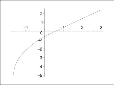
Figure 1: The temperature versus horizon radius in logarithmic scale for $n=8$, $\hat{\alpha}_{0}=1$, $\hat{\alpha}_{2}=0.2$, $\hat{\alpha}_{3}=0.05$, $\hat{\eta}_{2}=0.5$ and $\hat{\eta}_{3}=-0.2$.

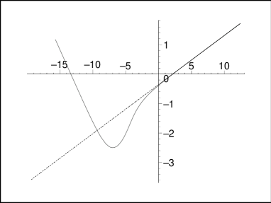
Figure 2: The temperature versus entropy in logarithmic scale for $n=8$, $\hat{\alpha}_{0}=1$, $\hat{\alpha}_{2}=0.2$ and $\hat{\alpha}_{3}=0.05$ with $\hat{\eta}_{2}=0.5$ and $\hat{\eta}_{3}=0.1$ (line), and $\hat{\eta}_{2}=\hat{\eta}_{3}=0$ (dotted).

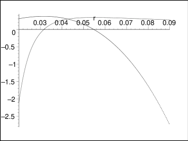
Figure 3: $10^{-2}dT/dS$ (line) and $10^{6}F$ (dotted) versus $r_{h}$ for $n=8$, $\hat{\alpha}_{0}=1$, $\hat{\alpha}_{2}=0.2$, $\hat{\alpha}_{3}=0.05$, $\hat{\eta}_{2}=0.5$ and $\hat{\eta}_{3}=0.006$.

The local stability of a thermodynamic system may be performed by analyzing the curve of $T$ versus $S$. Figure 2 depicts $\log T$ versus $\log S$ and shows that small black holes are unstable for positive $\hat{\eta}_{3}>\hat{\eta}_{3ext}$, while the very large black holes with nonconstant- curvature horizon are the same as black holes with constant curvature. To analyze the global stability, we should check the free energy of the black hole which is defined by $F\equiv M-TS$, whereby negative value ensures global stability Hawking . Substituting the expressions for mass, temperature and entropy from Eqs. (19), (32) and (31), one can perform the analysis of global stability. We plot the free energy versus the radius of black holes for $\hat{\eta}_{3}>\hat{\eta}_{3ext}$ in Fig. 3 which shows that small black holes are unstable both locally and globally, while there are medium black holes which may be locally stable, but they are globally unstable. So, in contrast to the case of $\kappa=0$ black holes with constant-curvature horizon which are stable Dehghani , the black hole solutions here may have unstable phases both locally and globally.

VI Concluding Remarks

In this paper, we assumed that the $n$-dimensional spacetime is a cross product of the two-dimensional Lorentzian spacetime and an $(n-2)$-dimensional nonconstant space. We found that the nontrivial Weyl tensor of such exotic horizons is exposed to the bulk dynamics through the higher- order Lovelock terms, severely constraining the allowed horizon geometries and adding a novel chargelike parameter to the black hole potential. Indeed, we found that the third-order Lovelock gravity can have a new class of black hole solutions with nonconstant-curvature horizons provided one imposes two conditions on the Weyl tensor. The first condition is the one which has been introduced by Dotti and Gleiser Dotti in Gauss-Bonnet gravity, while the second one is an additional condition involving the Weyl tensor of the horizon manifold with the advantage of higher curvature terms appearing in third-order Lovelock equations. This leads to a new class of static asymptotically flat and (A)dS black hole solutions. It is worth comparing our result with the already existing results in the literature. First, while in EGB gravity with an arbitrary Gauss-Bonnet coefficient only one condition is imposed on the Weyl tensor of Einstein horizon Dotti , here we faced with two conditions on the Weyl tensor of Einstein horizon. Second, as in the case of Gauss-Bonnet gravity with an arbitrary coupling constant we found that the horizon should be an Einstein manifold. However, for the cases when there is a unique maximally symmetric solution, the base manifold acquires more freedom Dot2 ; Bog ; Oliv1 ; Can ; Oliv2 . Third, while only one parameter appears in the solutions of Lovelock gravity in the Chern-Simons case Oliv1 or third- and higher-order Lovelock Born-Infeld gravity Can ; Oliv2 , here we encountered with two new different chargelike parameters $\hat{\eta}_{2}$ and $\hat{\eta}_{3}$. Thus, one may expect that in the case of Lovelock gravity with arbitrary Lovelock coefficients the number of charge-like parameters $\hat{\eta}_{p}$’s will increase as the order of Lovelock gravity becomes larger.

The thermodynamics of these black hole solutions have been investigated by calculating the temperature and the entropy through the use of the Wald formula. We found that the thermodynamic quantities satisfy the first law of thermodynamics. In contrast to the black holes of Lovelock gravity with constant curvature horizons, we found that there may exist extreme black holes with nonconstant-curvature horizon. We also found that the effect of the Weyl tensor in the metric and the expressions for temperature and entropy, lead to new features of the solutions that do not appear for the solutions of second-order Lovelock gravity with nonconstant-curvature horizons or in higher-order Lovelock gravity with constant-curvature ones. In order to show the main differences of black holes with constant- and nonconstant-curvature horizons, we went through the details of thermodynamics and stability analysis of black holes with $\kappa=0$. First, we found that the entropy does not obey the area law as a consequence of $\hat{\eta}_{2}$ appearing in the entropy expression. Second, we found that there may exist extreme black hole. Moreover, black holes with nonconstant-curvature horizons have an unstable phase both locally and globally, while those with constant-curvature horizons are stable both locally and globally Dehghani . But, it is worth mentioning that very large black holes with constant- and nonconstant-curvature horizons have the same features.

- (1) D. Lovelock, J. Math. Phys. 12, 498 (1971).
- (2) M. B. Greens, J. H. Schwarz, and E. Witten, Superstring Theory (Cambridge University Press, Cambridge, England, 1987); D. Lust and S. Theusen, Lectures on String Theory (Springer, Berlin, 1989); J. Polchinski, String Theory (Cambridge University Press, Cambridge, England, 1998).
- (3) D. G. Boulware and S. Deser, Phys. Rev. Lett. 55, 2656 (1985); J. T. Wheeler, Nucl. Phys. B268, 737 (1986); R. G. Cai, Phys. Rev. D 65, 084014 (2002).
- (4) Y. Brihaye and E. Radu, Phys. Lett. B 661, 167 (2008); S. Nojiri, S. D. Odintsov, and S. Ogushi, Phys. Rev. D 65, 023521 (2002); Y. Brihaye and E. Radu, J. High Energy Phys. 09 (2008) 006.
- (5) M. H. Dehghani and R. B. Mann, Phys. Rev. D 72, 124006 (2005); P. Mora, R. Olea, R. Troncoso, and J. Zanelli, J. High Energy Phys. 06 (2004) 036.
- (6) M. H. Dehghani and R. B. Mann, Phys. Rev. D 72, 124006 (2005); M. H. Dehghani and M. Shamirzaie, Phys. Rev. D 72, 124015 (2005); M. H. Dehghani and R. B. Mann, Phys. Rev. D 73, 104003 (2006).
- (7) R. G. Cai, L.M. Cao, Y. P. Hu, and S. P. Kim, Phys. Rev D 78, 124012 (2008); S.H. Mazharimousavi and M. Halilsoy, Phys. Lett. B 665, 125 (2008).
- (8) M. H. Dehghani and N. Farhangkhah, Phys. Rev. D 78, 064015 (2008); M. H. Dehghani and N. Farhangkhah, Phys. Lett. B 674, 243 (2009).
- (9) M. Ozkan and Y. Pang, J. High Energy Phys. 03 (2013) 158; 07 (2013) 152(E).
- (10) M. Kulaxizi and A. Parnachev, Phys. Rev. D 82, 066001 (2010); X.O. Camanho, J. D. Edelstein and M. F. Paulos, J. High Energy Phys. 05 (2011) 127.
- (11) X.O. Camanho, J. D. Edelstein, and M. F. Paulos, J. High Energy Phys. 05 (2011) 127; M. Brigante, H. Liu, R. C. Myers, S. Shenker, and S. Yaida, Phys. Rev. Lett. 100, 191601 (2008) ; Phys. Rev. D 77, 126006 (2008); J. de Boer, M. Kulaxizi, and A. Parnachev, J. High Energy Phys. 03 (2010) 087; X.O. Camanho and J. D. Edelstein, J. High Energy Phys. 06 (2010) 099; X.O. Camanho and J. D. Edelstein, J. High Energy Phys. 04 (2010) 007; A. Buchel, J. Escobedo, R. C. Myers, M. F. Paulos, A. Sinha, and M. Smolkin, J. High Energy Phys. 03 (2010) 111; J. de Boer, M. Kulaxizi and A. Parnachev, J. High Energy Phys. 06 (2010) 008.
- (12) R. G. Cai, Phys. Lett. B 582, 237 (2004); C. Garraffo and G. Giribet, Mod. Phys. Lett. A 23, 1810 (2008); C. Charmousis, Lect. Notes Phys. 769, 299 (2009); R. G. Cai and S. P. Kim, J. High Energy Phys. 02 (2005) 050; T. Padmanabhan and A. Paranjape, Phys. Rev. D 75, 064004 (2007).
- (13) H. Maeda, S. Willison, and S. Ray, Classical Quantum Gravity 28, 165005 (2011).
- (14) D. Kastor, S. Ray, and J. Traschen, Classical Quantum Gravity 27 235014 (2010).
- (15) D. N. Page, Phys. Lett. B 79, 235 (1978).
- (16) Y. Hashimoto, M. Sakaguchi and Y. Yasui, Commun. Math. Phys. 257, 273 (2005).
- (17) C. Bohm, Invent. Math. 134, 145 (1998).
- (18) G. Gibbons and S. A. Hartnoll, Phys. Rev. D 66, 064024 (2002).
- (19) H. Lu, D. N. Page, and C. N. Pope, Phys. Lett. B 593, 218 (2004).
- (20) J. P. Gauntlett, D. Martelli, J. F. Sparks, and D. Waldram, Adv. Theor. Math. Phys. 8, 987 (2006).
- (21) G. W. Gibbons, S. A. Hartnoll, and Y. Yasui, Classical Quantum Gravity 21, 4697 (2004).
- (22) G. W. Gibbons, S. A. Hartnoll, and C. N. Pope, Phys. Rev. D 67, 084024 (2003).
- (23) G. W. Gibbons and S. A. Hartnoll, Phys. Rev. D 66, 064024 (2002).
- (24) G. Dotti and R. J. Gleiser, Phys. Lett. B 627, 174 (2005).
- (25) H. Maeda, Phys. Rev. D 81, 124007 (2010).
- (26) H. Maeda, M. Hassaine, and C. Martinez, J. High Energy Phys. 08 (2010) 123.
- (27) G. Dotti, J. Oliva, and R. Troncoso, Phys. Rev. D 75, 024002 (2007); G. Dotti, J. Oliva, and R. Troncoso, Phys. Rev. D 76, 064038 (2007); G. Dotti, J. Oliva, and R. Troncoso, Int. J. Mod. Phys. A 24, 1690 (2009); G. Dotti, J. Oliva, and R. Troncoso, Phys. Rev. D 82, 024002 (2010).
- (28) C. Bogdanos, C. Charmousis, B. Gouteraux, and R. Zegers, J. High Energy Phys. 10 (2009) 037.
- (29) J. Oliva, J. Math. Phys. 54, 042501 (2013).
- (30) R. Troncoso and J. Zanelli, Classical Quantum Gravity 17, 4451 (2000); R. Aros, M. Contreras, R. Olea, R. Troncoso, and J. Zanelli, Phys. Rev. D 62, 044002 (2000).
- (31) F. Canfora and A. Giacomini, Phys. Rev. D 82, 024022 (2010).
- (32) A. Anabalon, F. Canfora, A. Giacomini, and J. Oliva, Phys. Rev. D 84, 084015 (2011).
- (33) M. H. Dehghani and R. Pourhasan, Phys. Rev. D 79 064015 (2009).
- (34) J. D. Beckenstein, Phys. Rev. D 7, 2333 (1973); W. Hawking, Nature (London) 248, 30 (1974); G. W. Gibbsons and S. W. Hawking, Phys. Rev D 15, 2738 (1977).
- (35) M. Lu and M. B. Wise, Phys. Rev. D 47, R3095 (1993); M. Visser, Phys. Rev. D 48, 583 (1993).
- (36) R. M. Wald, Phys. Rev. D 48, 3427 (1993); V. Iyer and R. M. Wald, Phys. Rev. D 50, 846 (1994); T. Jacobson, G. Kang, and R. C. Myers, Phys. Rev. D 49, 6587 (1994).
- (37) R. C. Myers and B. Robinson, J. High Energy Phys. 08 (2010) 067.
- (38) T. Jacobson and R. C. Myers, Phys. Rev. Lett. 70, 3684 (1993); M. Visser,Phys. Rev. D 48, 5697 (1993); (1994).
- (39) S. W. Hawking and D. N. Page, Commun. Math. Phys. 87, 577 (1983).