On Correlated Defaults and Incomplete Information

Wai-Ki Ching Advanced Modeling and Applied Computing Laboratory, Department of Mathematics, The University of Hong Kong, Pokfulam Road, Hong Kong. Email: wching@hku.hk.    Jia-Wen Gu Corresponding author, Department of Mathematical Sciences, University of Copenhagen, Universitetsparken 5, DK-2100 Copenhagen, Denmark. Email: jwgu.hku@gmail.com.    Harry Zheng Department of Mathematics, Imperial College, London, SW7 2AZ, UK. Email: h.zheng@imperial.ac.uk.
Abstract

In this paper, we study a continuous time structural asset value model for two correlated firms using a two-dimensional Brownian motion. We consider the situation of incomplete information, where the information set available to the market participants includes the default time of each firm and the periodic asset value reports. In this situation, the default time of each firm becomes a totally inaccessible stopping time to the market participants. The original structural model is first transformed to a reduced-form model. Then the conditional distribution of the default time together with the asset value of each name are derived. We prove the existence of the intensity processes of default times and also give the explicit form of the intensity processes. Numerical studies on the intensities of the two correlated names are conducted for some special cases. We also indicate the possible future research extension into three names case by considering a special correlation structure.

Keywords: Correlated Defaults, Brownian Motions, Incomplete Information, Intensity Models.

1 Introduction

There are two strands of literature for modeling credit risk, namely, the structural firm value model originated by Black and Scholes [3] and Merton [16] and the reduced-form model by Jarrow and Turnbull [12, 13]. In the classical firm value approach the asset value of a firm is described by a geometric Brownian motion and the default is triggered when the asset value falls below a given default barrier level. In the reduced-form intensity-based approach, defaults are modeled as exogenous events and their arrivals are described by using random point processes and the default time is a totally inaccessible stopping time.

The fundamental idea behind the paper dates back to the seminal paper by Duffie and Lando [5] where a concrete example is given to show how a reduced-form model can be obtained from a structural model by restricting the information structure. They consider a noisy and discretely observed firm asset value in a continuous-time setting, where the firm asset value is given by a diffusion process. This idea and associated mathematical issue has been studied by Eillott, Jeanblanc and Yor [9], Guo, Jarrow and Zeng [8]. It has been shown in these papers that it is possible to transform a structural model with a predictable default time into a reduced-form model, with a totally inaccessible default time, by introducing “incomplete information”.

However, most of the papers focus on one dimensional diffusions, while less attention has been placed to the correlation structure in the incomplete information model with multiple firms. Giesecke [6] proposes a model of correlated multi-firm default with incomplete information. Bond investors can observe issuers’ assets and defaults, but not the default threshold levels which are only revealed at times of default. Stochastic dependence between default events is induced through correlated asset values and correlated default thresholds.

We study the correlation structure in an incomplete information framework with asset values of firms being driven by a two-dimensional correlated Brownian motion and with known default threshold levels. The available information set includes the periodic asset value reports and the default times which are totally inaccessible stopping times to the market participants. We can transform the original structural model into a reduced-form intensity-based model and find the correlation structure of the two firms under such a transformation.

The main contribution of this paper is that we investigate the transformation from a structural model to reduced-form model with “incomplete information” on multiple correlated assets, provide the analytical expression for the conditional distribution of the default time, and prove the existence of the intensity process of default times, together with its explicit form. This paper sheds some new lights on the form of suitable intensity processes for portfolio credit risk. Our findings show that it is more reasonable to consider a contagion model, in which interacting intensities are time-varying with decaying default impacts ([7, 19, 20]).

The remainder of the paper is organized as follows. In Section 2 we present our model framework and give our main result: the default intensity process characterizing the correlation structure of the two firms. In Section 3 we illustrate our results by some numerical examples. In Section 4 we give the proof of our main result and preliminary results concerning the conditional default time and asset value distributions. In Section 5 we give concluding remarks and point out further research issues on the three-name case.

2 The Model and the Main Result

Assume $(\Omega,P,\mathcal{F})$ is a given probability space. The asset value process of firm $i$ is given by $V_{i}$, $i=1,2$. Define $\tau_{i}$ the default time of firm $i$ by

$$\tau_{i}:=\inf\{t>0:V_{i}(t)\leq B_{i}\},\ i=1,2,$$

where $B_{i}$ the default threshold value of firm $i$ satisfying $0<B_{i}<V_{i}(0)$. Denote by $X_{i}(t)=\ln\frac{V_{i}(t)}{B_{i}}$ for $t\geq 0$ and ${\bf X}=(X_{1}(t),X_{2}(t))^{T}$, ${\bf X}^{T}$ is the transpose of ${\bf X}$. Assume ${\bf X}$ stisfies the SDE,

$$d{\bf X}(t)=\mbox{\boldmath$\mu$}dt+\Sigma d{\bf W}(t),$$ (1)

where ${\bf W}$ is a two-dimensional standard Brownian motion, $\mu$ is a constant vector and $\Sigma$ is a constant matrix given by

$$\Sigma=\left(\begin{array}[]{cc}\sigma_{1}\sqrt{1-\rho^{2}}&\sigma_{1}\rho\\ 0&\sigma_{2}\end{array}\right),$$

in which $\sigma_{i}>0$ is the volatility of $X_{i}$, and $\rho$ is the correlation coefficient satisfying $|\rho|\leq 1$. Note that $X_{i}(0)>0,i=1,2$. By the continuity of $X_{i}$, the default time of firm $i$ can be written equivalently as

$$\tau_{i}=\inf\{t>0:X_{i}(t)=0\},\quad i=1,2.$$

Assume investors receive periodic information, at some fixed time instants

$$0=t_{0}<t_{1}<t_{2}<\ldots<t_{k}<\ldots.$$

The information available to investors up to time $t$ is given by

$$\mathcal{F}_{t}:=\mathcal{F}_{X_{1}}\vee\mathcal{F}_{X_{2}}\vee\sigma(1_{\{\tau_{1}\leq s\}},1_{\{\tau_{2}\leq s\}},0\leq s\leq t),$$

where

$$\mathcal{F}_{X_{i}}(t):=\sigma\left(X_{i}(t_{j}),j=0,1,\ldots,k_{i}\quad{\rm with}\quad t_{k_{i}}\leq\min\{t,\tau_{i}\}<t_{k_{i}+1}\right),\quad i=1,2.$$

Even though $X_{i}$ is a diffusion process and $B_{i}$ is a constant, $\tau_{i}$ is a totally inaccessible stopping time as investors can only observe the information of $X_{i}$ at discrete times $t_{k},k=0,1,\ldots$, and not the information of $X_{i}$ at all time $t\geq 0$ (which would lead to $\tau_{i}$ being a predictable stopping time). The main aim of this paper is to investigate the transformation from a structural model to a reduced-form model with this new information flow on two assets and deal with defaults with specified correlation structure.

We reformulate the problem by using a transformation proposed in Iyengar [11] and Metzler [17] and the default times $\tau_{i}\ (i=1,2)$ can be redefined. Let ${\bf Z}(t)=\Sigma^{-1}{\bf X}(t)$, we have

$$d{\bf Z}(t)={\bf m}dt+d{\bf W}(t),$$

where ${\bf m}=\Sigma^{-1}\mbox{\boldmath$\mu$}.$ The equivalent default times can be redefined as follows:

$$\left\{\begin{array}[]{ll}\tau_{1}&=\inf\left\{t>0:Z_{1}(t)=-\frac{\rho}{\sqrt{1-\rho^{2}}}Z_{2}(t)\right\},\\ \tau_{2}&=\inf\left\{t>0:Z_{2}(t)=0\right\}.\end{array}\right.$$

Denote by

$$\alpha=\left\{\begin{array}[]{ll}\pi+\tan^{-1}\left(-\frac{\sqrt{1-\rho^{2}}}{\rho}\right),&\rho>0,\\ \frac{\pi}{2},&\rho=0,\\ \tan^{-1}\left(-\frac{\sqrt{1-\rho^{2}}}{\rho}\right),&\rho<0.\end{array}\right.$$

We have $\alpha\in(0,\pi)$. Define

$${\tau:=\min(\tau_{1},\tau_{2})}.$$

Then $\tau$ is the first exit time of ${\bf Z}$ from the wedge

$$\Omega_{\alpha}:=\{(r\cos\theta,r\sin\theta)^{T}:r>0,0<\theta<\alpha\}$$

with the initial position of ${\bf Z}$ given by

$${\bf z}_{t_{0}}:={\bf Z}(0)=\Sigma^{-1}{\bf X}(0)=(r_{0}\cos\theta_{0},r_{0}\sin\theta_{0})^{T},\quad{\rm where}\quad 0<\theta_{0}<\alpha.$$

The unconditional joint distributions of $({\bf Z}(\tau),\tau)$ and $(\tau_{1},\tau_{2})$ are first derived in Iyengar [11] and corrected in Metzler [17]. The next theorem states their remarkable results.

Theorem 1

(Iyengar [11] and Metzler [17]) For ${\bf m}=(m_{1},m_{2})^{T}\in\mathcal{R}^{2}$,

$$P({\bf Z}(\tau)\in d{\bf z},\tau\in dt)=f(r,t,{\bf z}_{t_{0}})drdt,$$ (2)

where ${\bf z}=(r\cos\alpha,r\sin\alpha)^{T}$ and

$$f(r,t,{\bf z}_{t_{0}})=\exp\left({\bf m}^{T}[(r\cos\alpha,r\sin\alpha)^{T}-{\bf z}_{0}]-\frac{|{\bf m}|^{2}s}{2}\right)b(r,t,{\bf z}_{t_{0}})$$ (3)

and

$$b(r,t,{\bf z}_{t_{0}})=\frac{\pi}{\alpha^{2}tr}\exp\left(-\frac{r^{2}+r_{0}^{2}}{2t}\right)\sum_{n=1}^{\infty}n\sin\left(\frac{n\pi(\alpha-\theta_{0})}{\alpha}\right)I_{\frac{n\pi}{\alpha}}\left(\frac{rr_{0}}{t}\right)$$ (4)

and $I_{v}$ is the modified Bessel function of the first kind of order $v$, i.e.,

$$I_{v}(z)=\sum_{k=0}^{\infty}\frac{(\frac{1}{2}z)^{2k+v}}{k!\Gamma(v+k+1)}.$$ (5)

For $s<t$, let

$$g(s,t,{\bf z}_{t_{0}})=\int_{0}^{\infty}f(r,s,{\bf z}_{t_{0}})\pi(r\sin\alpha,t-s)dr,$$ (6)

where

$$\pi(x,h)=\frac{x}{\sqrt{2\pi h^{3}}}\exp\left(-\frac{(x+m_{2}h)^{2}}{2h}\right).$$ (7)

We have

$$P(\tau_{1}\in ds,\tau_{2}\in dt)=g(s,t,{\bf z}_{t_{0}})dsdt.$$ (8)
Remark 2

The function $\pi$ in Theorem 1 is the density of the hitting time to zero at time $h$ of a single Brownian motion with drift $m_{2}$ and initial value $x$. One can easily check by taking the partial derivative of $\pi(x,h)$ that, for fixed $h>0$, $\pi(.,h)$ achieves its maximum at $x=\frac{1}{2}\left(\sqrt{m_{2}^{2}h^{2}+4h}-m_{2}h\right)$ and for fixed $x>0$, $\pi(x,.)$ achieves its maximum at $h=\sqrt{\frac{x^{2}}{m_{2}^{2}}+\frac{9}{4m_{2}^{4}}}-\frac{3}{2m_{2}^{2}}$.

The conditional distributions of $\tau_{i}$ and $Z_{i}$, can be derived and characterized with the given information flow, see Lemmas 8 and 9 in Section 4.

The main objective of this paper is to find the intensity process $\lambda_{i}$ of $\tau_{i}$, given the filtration $\mathcal{F}_{u}$. The default time $\tau_{i}$ has an intensity process $\lambda_{i}$ with respect to the filtration $\mathcal{F}_{u}$ if $\lambda_{i}$ is a non-negative progressively measurable process satisfying

$$\int_{0}^{t}\lambda_{i}(u)du<\infty$$

a.s. for all $t$, such that

$$1_{\{\tau_{i}\leq t\}}-\int_{0}^{t}\lambda_{i}(u)du,t\geq 0$$

is an $\mathcal{F}_{t}$-martingale. Since investors receive periodic asset information at times $t_{k},k=0,1,\ldots$, the values ${\bf z}_{t_{k}}:={\bf Z}(t_{k})=(r_{k}\cos\theta_{k},r_{k}\sin\theta_{k})^{T}$ are known at $t_{k}$.

We can now state the main result of the paper.

Theorem 3

For $t_{j}\leq u<t_{j+1}$, the default intensity process of $\tau_{2}$ exists and is given by

$$\begin{array}[]{ll}\lambda_{2}(u)=&\displaystyle 1_{\{\tau_{2}>u\}}\cdot 1_{\{\tau_{1}>u\}}\left(\frac{\pi({z}_{t_{j}}^{(2)},u-t_{j})-\int_{0}^{u-t_{j}}g(s,u-t_{j},{\bf z}_{t_{j}})ds}{\int_{\Omega_{\alpha}}h(r,\theta,u-t_{j},{\bf z}_{t_{j}})drd\theta}\right)\\ &\displaystyle+1_{\{t_{j}\leq s<u\}}\cdot 1_{\{\tau_{2}>u\}}\cdot 1_{\{\tau_{1}=s\}}\left(\frac{g(s-t_{j},u-t_{j},{\bf z}_{t_{j}})}{\int_{u-t_{j}}^{\infty}g(s-t_{j},t,{\bf z}_{t_{j}})dt}\right)\\ &\displaystyle+1_{\{\tau_{2}>u\}}\cdot 1_{\{\tau_{1}<t_{j}\}}\left(\frac{\pi({z}_{t_{j}}^{(2)},u-t_{j})}{\int_{u-t_{j}}^{\infty}\pi({z}_{t_{j}}^{(2)},t)dt}\right),\end{array}$$ (9)

where ${z}_{t_{j}}^{(2)}$ represents the second component of ${\bf z}_{t_{j}}$, functions $g$ and $\pi$ are defined in (6) and (7), respectively, and $h$ is defined by

$$\begin{array}[]{lll}h(r,\theta,t,{\bf z}_{j})&=&\exp\left({\bf m}^{T}[(r\cos\theta,r\sin\theta)^{T}-{\bf z}_{j}]-\frac{|{\bf m}|^{2}t}{2}\right)\frac{2r}{t\alpha}\times\\ &&\exp\left(-\frac{r^{2}+r^{2}_{j}}{2t}\right)\sum_{n=1}^{\infty}\sin(\frac{n\pi\theta}{\alpha})\sin(\frac{n\pi\theta_{j}}{\alpha})I_{\frac{n\pi}{\alpha}}(\frac{rr_{j}}{t}).\end{array}$$ (10)

To derive the intensity process of default time $\tau_{1}$, we perform the transformation $\tilde{\bf W}=\tilde{T}{\bf W}$, $\tilde{\bf Z}=\tilde{T}\Sigma^{-1}{\bf X}$ and $\tilde{\bf m}=\tilde{T}\Sigma^{-1}\mbox{\boldmath$\mu$}$, where

$$\tilde{T}=\left(\begin{array}[]{cc}-\rho&\sqrt{1-\rho^{2}}\\ \sqrt{1-\rho^{2}}&\rho\end{array}\right).$$

Then we have

$$d\tilde{\bf Z}=\tilde{\bf m}dt+d\tilde{\bf W}.$$

The default times $\tau_{i},i=1,2$, are given by

$$\left\{\begin{array}[]{ll}\tau_{1}=\inf\{t>0:\tilde{Z}_{2}(t)=0\}\\ \tau_{2}=\inf\{t>0:\tilde{Z}_{1}(t)=-\frac{\rho}{\sqrt{1-\rho^{2}}}\tilde{Z}_{2}(t)\}.\end{array}\right.$$

Following the same argument, we have

Corollary 4

The intensity process of default time $\tau_{1}$ exists and is given by, for $t_{j}\leq u<t_{j+1}$,

$$\begin{array}[]{lll}\lambda_{1}(u)&=&\displaystyle 1_{\{\tau_{1}>u\}}\cdot 1_{\{\tau_{2}>u\}}\left(\frac{\pi(\tilde{z}_{t_{j}}^{(2)},u-t_{j})-\int_{0}^{u-t_{j}}\tilde{g}(s,u-t_{j},\tilde{\bf z}_{t_{j}})ds}{\int_{\Omega_{\alpha}}\tilde{h}(r,\theta,u-t_{j},\tilde{\bf z}_{t_{j}})drd\theta}\right)\\ &&\displaystyle+1_{\{t_{j}\leq s<u\}}\cdot 1_{\{\tau_{1}>u\}}\cdot 1_{\{\tau_{2}=s\}}\left(\frac{\tilde{g}(s-t_{j},u-t_{j},\tilde{\bf z}_{t_{j}})}{\int_{u-t_{j}}^{\infty}\tilde{g}(s-t_{j},t,\tilde{\bf z}_{t_{j}})dt}\right)\\ &&\displaystyle+1_{\{\tau_{1}>u\}}\cdot 1_{\{\tau_{2}<t_{j}\}}\left(\frac{\pi(\tilde{z}_{t_{j}}^{(2)},u-t_{j})}{\int_{u-t_{j}}^{\infty}\pi(\tilde{z}_{t_{j}}^{(2)},t)dt}\right),\end{array}$$ (11)

where $\tilde{g}$ and $\tilde{h}$ are the same as $g$ and $h$, respectively, with ${\bf m}$ replaced by $\tilde{\bf m}$.

Remark 5

Theorem 3 and Corollary 4 show that the operational status of one firm can have substantial impact to the default of another firm. The default of one firm may cause a significant change of default rate of another firm for a certain period and its impact decreases after new information is released. Starting from a reduced-form intensity model for portfolio credit risk, this theorem also shows that it is more reasonable to consider a contagion model, in which interacting intensities are time-varying with decaying default impacts.

The proof of Theorem 3 is given in Section 4. We first prove the case with single observation, and then extend to multiple observations. We show the existence of the local default rate and, with the help of Aven’s conditions [2], establish this local default rate being the intensity process. The proof relies on the hitting time distribution of correlated Brownian motions, see Iyengar [11] and Metzler [17]. We also derive the conditional distributions of default times and asset values as a by-product (Lemma 8, 9).

3 Valuation and Approximation

3.1 Valuation in Some Special Cases and Implications

It is not easy to find the intensities $\lambda_{1}$ and $\lambda_{2}$ as the results in (9) and (11) are complicated and In this section, we give the valuation of $\lambda_{1}$ and $\lambda_{2}$ in some special cases and give some insights about the correlation structure under incomplete information. Note that Iyengar [11] and Metzler [17] derive the expressions (6) and (10) by solving a PDE. When the correlation $\rho$ of the two Brownian motions satisfies certain conditions, the expressions in (6) and (10) can be simplified. Let

$$\rho_{k}=-\cos\left(\frac{\pi}{k}\right)\quad{\rm and}\quad\alpha_{k}=\frac{\pi}{k},\quad k=1,\ldots$$

For a fixed $k$, $T_{j}$ is the matrix representing the reflection across the line

$$y=x\tan(j\alpha_{k})\quad{\rm and}\quad S_{j}=T_{j}S_{j-1},\ \ S_{0}=I.$$

Then we have

Theorem 6

(Iyengar [11]) If ${\bf m}={\bf 0}$, $\alpha=\alpha_{k}$ and ${\bf z}\in\Omega_{\alpha}$, then

$$P_{\{{\bf m}={\bf 0}\}}({\bf Z}(t)\in d{\bf z},\tau>t)=\frac{1}{t}\sum_{j=0}^{2k-1}(-1)^{j}\Psi\left(\frac{z_{0}-S_{j}{\bf z}}{\sqrt{t}}\right)d{\bf z},$$

where $\Psi({\bf x})=(2\pi)^{-1}\exp(\frac{-{\bf x}^{T}{\bf x}}{2})$.

As claimed in Iyengar [11] and verified in Blanchet-Scalliet and Patras [4],

$$P_{\{{\bf m}={\bf 0}\}}({\bf Z}(t)\in d{\bf z},\tau\in dt)=\frac{1}{2}\frac{\partial}{\partial{\bf n}}P_{\{{\bf m}={\bf 0}\}}({\bf Z}(t)\in d{\bf z},\tau>t)$$

where $\frac{\partial}{\partial{\bf n}}$ denotes the derivative in the direction of inward normal to the boundary $\partial\Omega_{\alpha}$ at point ${\bf z}$. This simplifies the computation of $b(r,t,{\bf z}_{0})$ in (4) as follows:

$$\begin{array}[]{lll}b(r,t,{\bf z}_{0})&=&\displaystyle\frac{1}{2t}\sum_{j=0}^{2k-1}(-1)^{j}\frac{\partial}{\partial{\bf n}}\Psi\left(\frac{{\bf z}_{0}-S_{j}{\bf z}}{\sqrt{t}}\right)\\ &=&\displaystyle\frac{1}{2t}\sum_{j=0}^{2k-1}(-1)^{j}\frac{\partial}{\partial{\bf n}^{\prime}}\Psi\left(\frac{\tilde{\bf z}_{0}-S_{j}{\bf z}}{\sqrt{t}}\right)\\ &=&\displaystyle\frac{1}{2t^{2}}\sum_{j=0}^{2k-1}(-1)^{j}\Psi\left(\frac{\tilde{\bf z}_{0}-S_{j}\tilde{\bf z}}{\sqrt{t}}\right)({\tilde{\bf z}_{0}}^{T}S_{j}{\bf e}_{2}),\end{array}$$ (12)

where ${\bf n}=(\sin\alpha,-\cos\alpha)$, ${\bf n}^{\prime}=(0,1)$, $\tilde{\bf z}_{0}=(r_{0}\cos\tilde{\theta}_{0},r_{0}\sin\tilde{\theta}_{0})$ with $\tilde{\theta}_{0}=\alpha-\theta_{0}$ and $\tilde{\bf z}=(r,0)$. We can also get a simple expression for h, defined in (10), as

$$h(r,\theta,t,{\bf z}_{0})=\exp\left({\bf m}^{T}[(r\cos\theta,r\sin\theta)^{T}-{\bf z}_{0}]-\frac{|{\bf m}|^{2}t}{2}\right)\frac{r}{t}\sum_{j=0}^{2k-1}(-1)^{j}\Psi\left(\frac{{\bf z}_{0}-S_{j}{\bf z}}{\sqrt{t}}\right).$$ (13)

By combining Eq.s (9), (11), (12), and (13), we conduct a numerical study to investigate, in the special cases ($\alpha=\alpha_{k}$), the interacting intensities of the two firms.

Remark 7

We have $\rho_{k}\rightarrow-1$ as $k\rightarrow\infty$, which implies that when $\rho$ is sufficiently close to $-1$, one can approximate the intensity process by that of $\rho_{k}$, where $\rho_{k}\leq\rho<\rho_{k+1}$.

We next give two numerical examples to illustrate the infection effect of the two firms. The data used are ${\bf x}_{0}=(9,10)^{T},\ \mbox{\boldmath$\mu$}=(2,3)^{T},\ \sigma_{1}=4,\ {\rm and}\ \sigma_{2}=5.$

Figure 1 presents intensity process $\lambda_{2}$ of default time $\tau_{2}$ of firm B in independent case ($\rho=0$), negative correlated case ($\rho=-0.5$) and highly negative correlated case ($\rho=-0.7$), where the time length between two observations ($\Delta t$) is $10$ (years) and the default time of firm A is $\tau_{1}=2$. Note that when $\rho=0$, $\lambda_{2}$ is not affected by the default event of firm A, which is consistent with our expectation as firm A and B are independent of each other. The default of firm A has a substantial impact on the intensity process $\lambda_{2}$ when $\rho\neq 0$, which drops sharply as the two firms are negative correlated. The default of firm A has a even more significant impact on firm B when they are highly negative correlated. The figure also reveals a fact that before a default is observed, the intensity process $\lambda_{2}$ in the correlated case is nearly the same as that in the independent case.
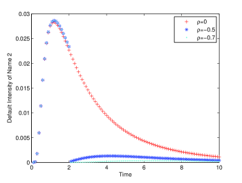
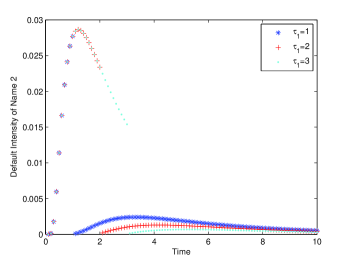
Refer to caption
Figure 1: Default Intensity process $\lambda_{2}$ when $\tau_{1}=2$

Figure 2 presents $\lambda_{2}$ with varying default times of firm A with the same data and $\rho=-0.5$. We observe that as two firms are negative correlated, $\lambda_{2}$ experiences a sharp drop at the default time of firm A, after which $\lambda_{2}$ increases slightly as the default impact decreases. In the long run, $\lambda_{2}$ tends to zero as the drift is positive.

Refer to caption
Figure 2: Default Intensities of firm B where $\rho=-0.5$

3.2 Approximation in General Cases

We now focus on the interval $[t_{0},t_{1}]$. To simplify the notations, we write $g(s,t,{\bf z}_{0})$ as $g(s,t)$ and $h(r,\theta,t,{\bf z}_{0})$ as $g(r,\theta,t)$ in the rest of the paper. The evaluation of the intensity of each firm by taking the integration of $g(s,t)$ and $h(r,\theta,t)$ incurs a large computational cost. We employ the numerical method in Kou and Zhong [15], Rogers and Shepp [18] to evaluate the Laplace transform of $(\tau_{1},\tau_{2})$ and $\tau$. Using the inverse Laplace transform, we can find the distributions of $(\tau_{1},\tau_{2})$ and $\tau$. The terms in the expression of $\lambda_{2}(t)$ in Theorem 14 can be expressed as:

$$\left\{\begin{array}[]{l}\displaystyle\int_{0}^{u}g(s,u)ds=\frac{dP(\tau_{1}\leq s,\tau_{2}\leq t)}{dt}\left|{}_{(s,t)=(u,u)}\right.\\ \displaystyle\int_{u}^{\infty}g(s,v)dv=\frac{dP(\tau_{1}\leq s,\tau_{2}>u)}{ds},\\ \displaystyle g(s,u)=\frac{d^{2}P(\tau_{1}\leq s,\tau_{2}\leq t)}{dsdt},\\ \displaystyle\int_{\Omega_{\alpha}}h(r,\theta,u)drd\theta=P(\tau>u).\\ \end{array}\right.$$

The Laplace transform of the joint distribution of $(\tau_{1},\tau_{2})$ is given by

$$E[e^{-p_{1}\tau_{1}-p_{2}\tau_{2}}\mid{\bf X}(0)=(x_{1},x_{2})].$$ (14)

The solution to the following PDE

$$\mathcal{L}(u)(x_{1},x_{2})=(p_{1}+p_{2})u$$

where

$$\mathcal{L}=\frac{1}{2}\sigma_{1}^{2}\frac{\partial^{2}}{\partial x_{1}^{2}}+\rho\sigma_{1}\sigma_{2}\frac{\partial^{2}}{\partial x_{1}\partial x_{2}}+\frac{1}{2}\sigma_{2}^{2}\frac{\partial^{2}}{\partial x_{2}^{2}}+\mu_{1}\frac{\partial}{\partial x_{1}}+\mu_{2}\frac{\partial}{\partial x_{2}}$$

if exists, has the representation given in Eq. (14). In their innovative papers [15, 18], Kontorovich-Lebedev transform and finite Fourier transform are proposed to solve the PDE for (14). We use these methods to solve the PDE and find the joint distribution numerically. We can then approximate the intensity process for general $\rho$.

Figure 3 presents the approximate and the exact intensity process $\lambda_{2}$ in independent case. Data used are ${\bf x}_{0}=(1,1)^{T},\ \mbox{\boldmath$\mu$}=(0.1,-0.2)^{T},\ \sigma_{1}=1.2,\ {\rm and}\ \sigma_{2}=0.5.$ Numerical tests show that the approximation method can give a good approximation of the default intensity process.

Refer to caption
Figure 3: Default Intensity Process $\lambda_{2}$ when $\rho=0$

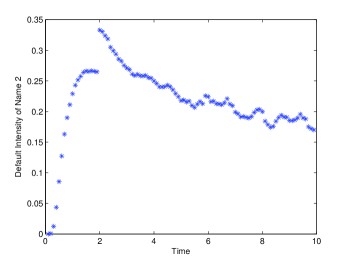
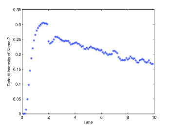
To give examples of the default intensity in general cases, we adopt the same parameters and assume the correlated parameter $\rho$ equals $0.1$ and $-0.1$. From Figures 5 and 6, we can observe a sharp upward jump in $\lambda_{2}$ when firm A defaults at time $\tau_{1}=2$ if $\rho=0.1$ and a sharp downward jump if $\rho=-0.1$. This is consistent with our intuition.

Refer to caption
Figure 4: Default Intensity Process $\lambda_{2}$ when $\tau_{1}=2$ and $\rho=0.1$
Refer to caption
Figure 5: Default Intensity Process $\lambda_{2}$ when $\tau_{1}=2$ and $\rho=-0.1$

4 Proof of Theorem 3

4.1 Preliminary Results

The objective of this subsection is to obtain the conditional distributions of $\tau_{i}$ and $Z_{i}$ ($i=1,2$) given $\mathcal{F}_{u}$. For simplicity, we assume that $t_{0}<u<t_{1}$. We only need to derive the conditional distribution of $\tau_{2}$ given $\mathcal{F}_{u}$, that of $\tau_{1}$ can be derived easily with a transformation. The derivation relies on the results given in Theorem 1.

We now give the conditional default time distribution given $\mathcal{F}_{u}$.

Lemma 8

For $0<s<u<v$, the conditional distribution of $\tau_{2}$ is given by,

$$\begin{array}[]{ll}1_{\{\tau_{2}>u\}}P(\tau_{2}\in dv\mid\mathcal{F}_{u})=&1_{\{\tau_{2}>u\}}\cdot 1_{\{\tau_{1}>u\}}\displaystyle\left(\frac{\pi(z_{0}^{(2)},v)-\int_{0}^{u}g(s,v)ds}{\int_{\Omega_{\alpha}}h(r,\theta,u)drd\theta}dv\right)\\ &+1_{\{\tau_{2}>u\}}\cdot 1_{\{\tau_{1}=s\}}\displaystyle\left(\frac{g(s,v)}{\int_{u}^{\infty}g(s,t)dt}dv\right),\end{array}$$ (15)

where $z_{0}^{(2)}$ is the second entry of ${\bf z}_{0}$ and $h(r,\theta,u)$ is given in Eq.(17).

Proof: By Bayes’ rule, for $s<u<v$, the conditional distribution of $\tau_{2}$ is given by

$$\begin{array}[]{ll}1_{\{\tau_{2}>u\}}\cdot P(\tau_{2}\in dv\mid\mathcal{F}_{u})=&1_{\{\tau_{2}>u\}}\cdot 1_{\{\tau_{1}>u\}}\cdot P(\tau_{2}\in dv\mid\tau>u)\\ &+1_{\{\tau_{2}>u\}}\cdot 1_{\{\tau_{1}=s\}}\cdot P(\tau_{2}\in dv\mid\tau_{2}>u,\tau_{1}=s).\end{array}$$ (16)

For the first term of the RHS of Eq. (16), we have

$$\begin{array}[]{lll}P(\tau_{2}\in dv\mid\tau>u)&=&\displaystyle\frac{P(\tau_{2}\in dv,\tau_{1}>u)}{P(\tau>u)}\\ &=&\displaystyle\frac{P(\tau_{2}\in dv)-P(\tau_{2}\in dv,\tau_{1}\leq u)}{P(\tau>u)}\\ &=&\displaystyle\frac{\pi(z_{0}^{(2)},v)-\int_{0}^{u}g(s,v)ds}{P(\tau>u)}dv.\end{array}$$

From Iyengar [11] and Metzler [17], we also have

$$P(\tau>u)=\int_{\Omega_{\alpha}}h(r,\theta,u)drd\theta,$$

where

$$\begin{array}[]{lll}h(r,\theta,t)&=&\displaystyle\frac{2r}{t\alpha}\exp\left(m_{1}(r\cos\theta-z_{0}^{(1)})+m_{2}(r\sin\theta-z_{0}^{(2)})-\frac{|{\bf m}|^{2}t}{2}\right)\exp\left(-\frac{r^{2}+r_{0}^{2}}{2t}\right)\times\\ &&\displaystyle\sum_{n=1}^{\infty}\sin\left(\frac{n\pi\theta}{\alpha}\right)\sin\left(\frac{n\pi\theta_{0}}{\alpha}\right)I_{\frac{n\pi}{\alpha}}\left(\frac{rr_{0}}{t}\right).\end{array}$$ (17)

Note that the second term of the RHS of Eq. (16) is

$$P(\tau_{2}\in dv\mid\tau_{2}>u,\tau_{1}=s)=\displaystyle\frac{P(\tau_{2}\in dv,\tau_{1}\in ds)}{P(\tau_{2}>u,\tau_{1}\in ds)}=\displaystyle\frac{g(s,v)}{\int_{u}^{\infty}g(s,t)dt}dv.$$

The result follows.

We also present the conditional distribution of $Z_{i}(u),i=1,2$ given the filtration $\mathcal{F}_{u}$. Again we give the conditional distribution of $Z_{2}(u)$, while the conditional distribution of $Z_{1}(u)$ can be derived similarly.

Lemma 9

For $0<s<u$,

$$\begin{array}[]{lll}1_{\{\tau_{2}>u\}}P(Z_{2}(u)\in dx\mid\mathcal{F}_{u})&=&1_{\{\tau_{2}>u\}}\cdot 1_{\{\tau_{1}>u\}}\displaystyle\left(\frac{\tilde{\pi}(x,z^{(2)}_{0},u)-p(x,u)}{\int_{\Omega_{\alpha}}h(r,\theta,u)drd\theta}dx\right)\\ &&+1_{\{\tau_{2}>u\}}\cdot 1_{\{\tau_{1}=s\}}\displaystyle\left(\frac{l(s,u,x)}{\int_{u}^{\infty}g(s,t)dt}dx\right),\end{array}$$ (18)

where

$$\left\{\begin{array}[]{lll}l(s,t,x)&=&\displaystyle\int_{0}^{\infty}f(r,s)\tilde{\pi}(x,r\sin\alpha,u-s)dr,\\ p(x,t)&=&\displaystyle\int_{0}^{t}l(s,t,x)ds,\\ \tilde{\pi}(x,x_{0},h)&=&\displaystyle\frac{1}{\sqrt{2\pi h}}\exp\left(-\frac{(x-x_{0}-m_{2}h)^{2}}{2h}\right)\left(1-\exp(-\frac{2x_{0}x}{h})\right).\end{array}\right.$$

Proof: By Bayes’ rule, one can obtain

$$\begin{array}[]{ll}1_{\{\tau_{2}>u\}}P(Z_{2}(u)\in dx\mid\mathcal{F}_{u})=&1_{\{\tau_{2}>u\}}\cdot 1_{\{\tau_{1}>u\}}P(Z_{2}(u)\in dx\mid\tau>u)\\ &+1_{\{\tau_{2}>u\}}\cdot 1_{\{\tau_{1}=s\}}P(Z_{2}(u)\in dx\mid\tau_{2}>u,\tau_{1}=s).\end{array}$$ (19)

We note that according to the density function of the first passage time and a straightforward calculation (see for instance Chapter 1 of Harrison [10]), the probability of a Brownian motion with drift $m_{2}$, conditioning on starting at some level $x_{0}$ at time 00, ends at level $x$ at time $h$ with running minimum being positive is

$$\tilde{\pi}(x,x_{0},h)=\displaystyle\frac{1}{\sqrt{2\pi h}}\exp\left(-\frac{(x-x_{0}-m_{2}h)^{2}}{2h}\right)\left(1-\exp(-\frac{2x_{0}x}{h})\right).$$

For the second term of Eq. (19),

$$P(Z_{2}(u)\in dx\mid\tau_{2}>u,\tau_{1}=s)=\displaystyle\frac{P(\tau_{2}>u,Z_{2}(u)\in dx,\tau_{1}\in ds)}{P(\tau_{1}\in ds,\tau_{2}>u)},$$

and

$$\begin{array}[]{lll}P(\tau_{2}>u,Z_{2}(u)\in dx,\tau_{1}\in ds)&=&\displaystyle\int_{0}^{\infty}f(r,s)P(\tau_{2}>u,Z_{2}(u)\in dx\mid Z_{2}(s)=r\sin\alpha)drds\\ &=&\displaystyle\int_{0}^{\infty}f(r,s)\tilde{\pi}(x,r\sin\alpha,u-s)drdxds\\ &=&l(s,u,x)dsdx.\end{array}$$

For the first term of Eq. (19),

$$\begin{array}[]{lll}P(Z_{2}(u)\in dx\mid\tau>u)&=&\displaystyle\frac{P(\tau>u,Z_{2}(u)\in dx)}{P(\tau>u)}\\ &=&\displaystyle\frac{P(\tau_{2}>u,Z_{2}(u)\in dx)-P(\tau_{1}\leq u,\tau_{2}>u,Z_{2}(u)\in dx)}{P(\tau>u)},\end{array}$$

where

$$P(\tau_{2}>u,Z_{2}(u)\in dx)=\tilde{\pi}(x,z^{(2)}_{0},u)dx,$$

and

$$P(\tau_{1}\leq u,\tau_{2}>u,Z_{2}(u)\in dx)=\int_{0}^{u}l(s,u,x)dsdx=p(x,u)dx.$$

The the result follows.

Given the survival to $u$, the above theorem gives us the conditional distribution of assets, because the conditional density of ${\bf V}(t)$ can be easily obtained from the conditional density of ${\bf Z}(t)$.

4.2 Existence and Explicit Form of $\lambda_{i}$

To prove Theorem 3, we first begin with single observations, i.e. $t_{0}<u<t_{1}$, and then extend to multiple observations. The intuitive meaning of the intensity is given by the local default rate,

$$\lim_{\delta u\rightarrow 0}\frac{1}{\delta u}P(\tau_{i}\in(u,u+\delta u]\mid\mathcal{F}_{u}).$$ (20)

To obtain the intensity process $\{\lambda_{i}(u)\}_{u\geq 0}$, we need the following lemmas.

Lemma 10

For a fixed $s$, $g(s,.)$ is continuous in $(s,+\infty)$.

Proof: By the following elementary inequalities

$$\sqrt{a+b}\pm\sqrt{a}\leq\sqrt{2(2a+b)},\ \ a>0,\ \ b>0,$$

and Remark 2, for a fixed $h>0$, $\pi(.,h)$ achieves its local maximum at

$$x=\frac{1}{2}\left(\sqrt{m^{2}_{2}h^{2}+4h}-m_{2}h\right).$$

We have

$$\pi(x,h)=\frac{x}{\sqrt{2\pi h^{3}}}\exp\left(-\frac{(x+m_{2}h)^{2}}{2h}\right)\leq\frac{\frac{1}{2}\left(\sqrt{m^{2}_{2}h^{2}+4h}-m_{2}h\right)}{\sqrt{2\pi h^{3}}}\leq\frac{\sqrt{m^{2}_{2}h+2}}{\sqrt{2\pi h^{2}}}.$$ (21)

For any $t>s$ and $n\in\mathcal{N}^{+}$,

$$g\left(s,t+\frac{1}{n}\right)=\int_{0}^{\infty}f(r,s)\pi\left(r\sin\alpha,t+\frac{1}{n}-s\right)dr,$$

where

$$\begin{array}[]{lll}f(r,s)\pi(r\sin\alpha,t+\frac{1}{n}-s)&\leq&\displaystyle f(r,s)\cdot\frac{\sqrt{m^{2}_{2}(t+\frac{1}{n}-s)+2}}{\sqrt{2\pi(t+\frac{1}{n}-s)^{2}}}\\ &\leq&\displaystyle f(r,s)\cdot\frac{\sqrt{m^{2}_{2}(t+1-s)+2}}{\sqrt{2\pi(t-s)^{2}}}.\end{array}$$

Since $f$ gives the joint density of $(\tau,{\bf Z}(\tau))$, we have

$$\int_{0}^{\infty}f(r,s)dr<\infty.$$

Using the Dominated Convergence Theorem (DCT) and the fact that $\pi$ is continuous in $(0,\infty)\times(0,\infty)$, we have

$$\begin{array}[]{lll}\displaystyle\lim_{n\rightarrow\infty}g\left(s,t+\frac{1}{n}\right)&=&\displaystyle\int_{0}^{\infty}\lim_{n\rightarrow\infty}f(r,s)\pi\left(r\sin\alpha,t+\frac{1}{n}-s\right)dr\\ &=&\int_{0}^{\infty}f(r,s)\pi(r\sin\alpha,t-s)dr\\ &=&g(s,t).\end{array}$$

Lemma 11

For modified Bessel function of the first kind of order $v$, $I_{v}$ (c.f. Eq. (5) ), we have for $z\in(0,1)$,

$$\sum_{n=1}^{\infty}nI_{\frac{n\pi}{2\alpha}}(z)\leq Cz^{\frac{\pi}{2\alpha}},$$

where we denote by $C$ a generic positive constant, not necessarily the same at each appearance in the rest of the paper.

Proof: For any positive real number $v$,

$$I_{v}(z)=\sum_{k=0}^{\infty}\frac{(\frac{1}{2}z)^{2k+v}}{k!\Gamma(v+k+1)}\leq\sum_{k=0}^{\infty}\frac{(\frac{1}{2}z)^{2k+v}}{k!}=e^{\frac{z^{2}}{4}}\left(\frac{1}{2}z\right)^{v}<e\left(\frac{1}{2}z\right)^{v}.$$

Therefore,

$$\sum_{n=1}^{\infty}nI_{\frac{n\pi}{2\alpha}}(z)<e\sum_{n=1}^{\infty}n\left(\frac{1}{2}z\right)^{\frac{n\pi}{2\alpha}}\leq\frac{e(1/2)^{\frac{\pi}{2\alpha}}z^{{}^{\frac{\pi}{2\alpha}}}}{[1-(z/2){{}^{\frac{\pi}{2\alpha}}}]^{2}}\leq\frac{e(1/2)^{\frac{\pi}{2\alpha}}z^{{}^{\frac{\pi}{2\alpha}}}}{[1-(1/2){{}^{\frac{\pi}{2\alpha}}}]^{2}}=Cz^{\frac{\pi}{2\alpha}}.$$

The next result characterizes the local default rate.

Lemma 12

For $0<s<u$ and $\{u_{n}\}$ a sequence decreasing to 00, we have

$$\begin{array}[]{ll}&\displaystyle\lim_{n\rightarrow\infty}\frac{1_{\{\tau_{2}>u\}}}{u_{n}}P(\tau_{2}\in(u,u+u_{n}]\mid\mathcal{F}_{u})\\ =&\displaystyle 1_{\{\tau_{2}>u\}}\cdot 1_{\{\tau_{1}>u\}}\left(\frac{\pi(z_{0}^{(2)},u)-\int_{0}^{u}g(s,u)ds}{\int_{\Omega_{\alpha}}h(r,\theta,u)drd\theta}\right)+1_{\{\tau_{2}>u\}}\cdot 1_{\{\tau_{1}=s\}}\left(\frac{g(s,u)}{\int_{u}^{\infty}g(s,v)dv}\right).\end{array}$$

Proof: By Theorem 8, for $s<u$, we have

$$\begin{array}[]{lll}1_{\{\tau_{2}>u\}}\cdot P(\tau_{2}\in(u,u+u_{n}]\mid\mathcal{F}_{u})=&\displaystyle 1_{\{\tau_{2}>u\}}\cdot 1_{\{\tau_{1}>u\}}\cdot\left(\frac{\int_{u}^{u+u_{n}}\pi(z_{0}^{(2)},v)dv-\int_{u}^{u+u_{n}}\int_{0}^{u}g(s,v)dsdv}{\int_{\Omega_{\alpha}}h(r,\theta,u)drd\theta}\right)\\ &\displaystyle+1_{\{\tau_{2}>u\}}\cdot 1_{\{\tau_{1}=s\}}\cdot\left(\frac{\int_{u}^{u+u_{n}}g(s,v)dv}{\int_{u}^{\infty}g(s,t)dt}\right).\end{array}$$ (22)

For the first term of the RHS of Eq. (22), we have

$$\lim_{n\rightarrow\infty}\frac{1}{u_{n}}\int_{u}^{u+u_{n}}\int_{0}^{u}g(s,v)dsdv=\int_{0}^{u}g(s,u)ds.$$ (23)

Eq. (23) can be proved as follows. Since $g$ is non-negative a.s., Fubini’s Theorem tells us that

$$\begin{array}[]{lll}\displaystyle\frac{1}{u_{n}}\int_{u}^{u+u_{n}}\int_{0}^{u}g(s,v)dsdv&=&\displaystyle\int_{0}^{u}\int_{0}^{\infty}f(r,s)\frac{1}{u_{n}}\left(\int_{u}^{u+u_{n}}\pi(r\sin\alpha,v-s)dv\right)drds\\ &=&\displaystyle\int_{0}^{u}\int_{0}^{\infty}f(r,s)\pi(r\sin\alpha,u+\eta_{n}-s)drds\\ &=&\displaystyle\int_{0}^{u}g(s,u+\eta_{n})ds,\end{array}$$ (24)

where $0<\eta_{n}<u_{n}$. Let $u^{*}\in(0,u)$ and $0<s<u<t$. For $s\in(0,u^{*})$, by Eq. (21)

$$g(s,t)\leq\frac{\sqrt{m^{2}_{2}(t-s)+2}}{\sqrt{2\pi}(t-s)}\int_{0}^{\infty}f(r,s)dr\leq\frac{\sqrt{m^{2}_{2}t+2}}{\sqrt{2\pi}(u-u^{*})}\int_{0}^{\infty}f(r,s)dr.$$ (25)

We can select $u^{*},\eta^{*}$ to be sufficiently close to $u$, such that for $t\in(u,\eta^{*})$ and $s\in[u^{*},u)$

$$\frac{r_{0}^{2}}{2s}\left(\frac{t-s}{t-s\cos 2\alpha}\right)\in(0,1).$$

This can be done since

$$t-s\cos 2\alpha=t-s+2s\sin^{2}\alpha\geq 2u^{*}\sin^{2}\alpha>0.$$

Then we claim that

g(s,t)Cstscos2α(ts)exp(|𝐦|2s2)n=1nsin(nπθ~0α)Inπ2α(r022ststscos2α)Cstscos2α(ts)exp(|𝐦|2s2)(r022ststscos2α)π2α(byLemma11)C(ts)π2α1[s(tscos2α)]12+π2αexp(|𝐦|2s2)Cu1+παexp(|𝐦|2u2)(ts)π2α1.𝑔𝑠𝑡𝐶𝑠𝑡𝑠2𝛼𝑡𝑠superscript𝐦2𝑠2superscriptsubscript𝑛1𝑛𝑛𝜋subscript~𝜃0𝛼subscript𝐼𝑛𝜋2𝛼superscriptsubscript𝑟022𝑠𝑡𝑠𝑡𝑠2𝛼missing-subexpression𝐶𝑠𝑡𝑠2𝛼𝑡𝑠superscript𝐦2𝑠2superscriptsuperscriptsubscript𝑟022𝑠𝑡𝑠𝑡𝑠2𝛼𝜋2𝛼byLemma11missing-subexpression𝐶superscript𝑡𝑠𝜋2𝛼1superscriptdelimited-[]𝑠𝑡𝑠2𝛼12𝜋2𝛼superscript𝐦2𝑠2missing-subexpression𝐶superscriptsuperscript𝑢1𝜋𝛼superscript𝐦2𝑢2superscript𝑡𝑠𝜋2𝛼1\begin{array}[]{lll}g(s,t)&\leq&\displaystyle\frac{C}{\sqrt{s}\sqrt{t-s\cos 2\alpha}(t-s)}\exp\left(\frac{|{\bf m}|^{2}s}{2}\right)\sum_{n=1}^{\infty}n\sin\left(\frac{n\pi\tilde{\theta}_{0}}{\alpha}\right)I_{\frac{n\pi}{2\alpha}}\left(\frac{r_{0}^{2}}{2s}\frac{t-s}{t-s\cos 2\alpha}\right)\\ &\leq&\displaystyle\frac{C}{\sqrt{s}\sqrt{t-s\cos 2\alpha}(t-s)}\exp\left(\frac{|{\bf m}|^{2}s}{2}\right)\left(\frac{r_{0}^{2}}{2s}\frac{t-s}{t-s\cos 2\alpha}\right)^{\frac{\pi}{2\alpha}}({\rm by\ Lemma\ \ref{Bessellemma}})\\ &\leq&\displaystyle\frac{C(t-s)^{\frac{\pi}{2\alpha}-1}}{[s(t-s\cos 2\alpha)]^{\frac{1}{2}+\frac{\pi}{2\alpha}}}\exp\left(\frac{|{\bf m}|^{2}s}{2}\right)\\ &\leq&\displaystyle\frac{C}{{u^{*}}^{1+\frac{\pi}{\alpha}}}\exp\left(\frac{|{\bf m}|^{2}u}{2}\right)(t-s)^{\frac{\pi}{2\alpha}-1}.\end{array} (26)

The first inequality in the RHS of Eq. (26) holds by first considering

$$\begin{array}[]{lll}&&f(r,s)\pi(r\sin\alpha,t-s)\\ &\leq&b(r,s)\exp\left(m_{1}(r\cos\alpha-z^{(1)}_{0})+m_{2}(r\sin\alpha-z^{(2)}_{0})-\frac{|{\bf m}|^{2}s}{2}\right)\times\\ &&\displaystyle\frac{r\sin\alpha}{\sqrt{2\pi(t-s)^{3}}}\exp\left(-\frac{r^{2}\sin^{2}\alpha}{2(t-s)}-m_{2}r\sin\alpha\right)\\ &=&\displaystyle b(r,s)\frac{r\sin\alpha}{\sqrt{2\pi(t-s)^{3}}}\exp\left(-\frac{r^{2}\sin^{2}\alpha}{2(t-s)}\right)\exp\left(m_{1}r\cos\alpha\right)\exp\left(-m_{1}z^{(1)}_{0}-m_{2}z^{(2)}_{0}-\frac{|{\bf m}|^{2}s}{2}\right)\\ &\leq&\displaystyle b(r,s)\frac{r\sin\alpha}{\sqrt{2\pi(t-s)^{3}}}\exp\left(-\frac{r^{2}\sin^{2}\alpha}{2(t-s)}\right)\times\\ &&\displaystyle\exp\left(\frac{r^{2}}{4s}+s(m_{1}\cos\alpha)^{2}\right)\exp\left(-m_{1}z^{(1)}_{0}-m_{2}z^{(2)}_{0}-\frac{|{\bf m}|^{2}s}{2}\right)\\ &\leq&\displaystyle b(r,s)\frac{r\sin\alpha}{\sqrt{2\pi(t-s)^{3}}}\exp\left(-\frac{r^{2}\sin^{2}\alpha}{2(t-s)}+\frac{r^{2}}{4s}\right)\exp\left(-m_{1}z^{(1)}_{0}-m_{2}z^{(2)}_{0}+\frac{|{\bf m}|^{2}s}{2}\right)\\ &=&\displaystyle\frac{\sqrt{\pi}\sin\alpha}{\sqrt{2(t-s)^{3}}\alpha^{2}s}\exp\left(-\frac{r^{2}_{0}}{2s}\right)\exp\left(-m_{1}z^{(1)}_{0}-m_{2}z^{(2)}_{0}+\frac{|{\bf m}|^{2}s}{2}\right)\\ &&\times\displaystyle\exp\left(-\frac{r^{2}}{4s}\frac{t-s\cos 2\alpha}{t-s}\right)\sum_{n=1}^{\infty}n\sin\left(\frac{n\pi\tilde{\theta}_{0}}{\alpha}\right)I_{\frac{n\pi}{\alpha}}(\frac{rr_{0}}{s})\\ &=&\displaystyle\frac{C}{\sqrt{(t-s)^{3}}s}\exp\left(-\frac{r^{2}_{0}}{2s}+\frac{|{\bf m}|^{2}s}{2}\right)\displaystyle\exp\left(-\frac{r^{2}}{4s}\frac{t-s\cos 2\alpha}{t-s}\right)\sum_{n=1}^{\infty}n\sin\left(\frac{n\pi\tilde{\theta}_{0}}{\alpha}\right)I_{\frac{n\pi}{\alpha}}(\frac{rr_{0}}{s}).\end{array}$$

By using the following identity (Abramowitz and Stegun [1]),

$$\int_{0}^{\infty}e^{-bt^{2}}I_{v}(at)dt=\frac{1}{2}\sqrt{\frac{\pi}{b}}\exp\left(\frac{a^{2}}{8b}\right)I_{\frac{v}{2}}\left(\frac{a^{2}}{8b}\right),$$
$$\begin{array}[]{lll}g(s,t)&=&\displaystyle\int_{0}^{\infty}f(r,s)\pi(r\sin\alpha,t-s)dr\\ &\leq&\displaystyle\frac{C}{\sqrt{s}\sqrt{t-s\cos 2\alpha}(t-s)}\exp\left(\frac{|{\bf m}|^{2}s}{2}\right)\exp\left(-\frac{r^{2}_{0}\sin^{2}\alpha}{t-s\cos 2\alpha}\right)\times\\ &&\displaystyle\sum_{n=1}^{\infty}n\sin\left(\frac{n\pi\tilde{\theta}_{0}}{\alpha}\right)I_{\frac{n\pi}{2\alpha}}\left(\frac{r_{0}^{2}}{2s}\frac{t-s}{t-s\cos 2\alpha}\right)\\ &\leq&\displaystyle\frac{C}{\sqrt{s}\sqrt{t-s\cos 2\alpha}(t-s)}\exp\left(\frac{|{\bf m}|^{2}s}{2}\right)\sum_{n=1}^{\infty}n\sin\left(\frac{n\pi\tilde{\theta}_{0}}{\alpha}\right)I_{\frac{n\pi}{2\alpha}}\left(\frac{r_{0}^{2}}{2s}\frac{t-s}{t-s\cos 2\alpha}\right).\end{array}$$

Combining Eq. (25) and Eq. (26), there exists $N_{0}\in\mathcal{N}^{+}$, such that for $n>N_{0}$,

$$g(s,u+\eta_{n})\leq f(u,u^{*},s),$$

where $f(u,u^{*},s)=$

$$\left\{\begin{array}[]{ll}\frac{\sqrt{m^{2}_{2}(u+u_{1})+2}}{\sqrt{2\pi}(u-u^{*})}\int_{0}^{\infty}f(r,s)dr,&s\in(0,u^{*}],\\ \frac{C}{{u^{*}}^{1+\frac{\pi}{\alpha}}}\exp\left(\frac{|{\bf m}|^{2}u}{2}\right)\left(1_{\{\alpha\leq\pi/2\}}(u+u_{1}-u^{*})^{\frac{\pi}{2\alpha}-1}+1_{\{\alpha>\pi/2\}}(u-s)^{\frac{\pi}{2\alpha}-1}\right),&s\in(u^{*},u),\end{array}\right.$$

is integrable on $(0,u)$ as a function of $s$. The DCT implies,

$$\lim_{n\rightarrow\infty}\int_{0}^{u}g(s,u+\eta_{n})ds=\int_{0}^{u}\lim_{n\rightarrow\infty}g(s,u+\eta_{n})ds=\int_{0}^{u}g(s,u)ds.$$

The result follows. Similarly $\pi$ is continuous in $(0,\infty)\times(0,\infty)$ we have

$$\frac{1}{u_{n}}\int_{u}^{u+u_{n}}\pi(z_{0}^{(2)},v)dv=\pi(z_{0}^{(2)},u+\xi_{n})\rightarrow\pi(z_{0}^{(2)},u)\quad{\rm as}\quad n\rightarrow\infty,$$

where $0<\xi_{n}<u_{n}$.

For the second term of the RHS of Eq. (22), by Lemma 10, when $n\rightarrow\infty$,

$$\frac{1}{u_{n}}\int_{u}^{u+u_{n}}g(s,v)dv=g(s,u+\psi_{n})\rightarrow g(s,u),$$

where $0<\psi_{n}<u_{n}$.

Before proving the main result of the subsection, we introduce the following result which is needed in the proof.

Lemma 13 (Aven [2])

Let $N(t)$ be a counting process adapted to $\{\mathcal{F}_{t}\}$ and assume there exists a process $\{\lambda(t)\}$ such that $\lambda(t)=\lim_{h_{n}\downarrow 0}Y_{n}$ where $Y_{n}=E[N(t+h_{n})-N(t)\mid\mathcal{F}_{t}]/h_{n}$, if the following conditions hold with $\{\lambda(t)\}$ and $\{y(t)\}$ non-negative and measurable processes:

  • for each $t$, $\lim_{n\rightarrow\infty}Y_{n}=\lambda(t)$,

  • for each $t$ there exists for almost all $\omega$ and $n_{0}=n_{0}(t,\omega)$, such that $|Y_{n}(s,\omega)-\lambda(s,\omega)|\leq y(s,\omega),s\leq t,n\geq n_{0}$,

  • $\int_{0}^{t}y(s)ds<\infty,0\leq t<\infty$.

Then $\{N(t)-\int_{0}^{t}\lambda(s)ds\}$ is an $\mathcal{F}_{t}$ martingale.

Theorem 14

The intensity process of $\tau_{2}$ is given by

$$\lambda_{2}(u)=1_{\{\tau_{2}>u\}}\cdot 1_{\{\tau_{1}>u\}}\left(\frac{\pi(z_{0}^{(2)},u)-\int_{0}^{u}g(s,u)ds}{\int_{\Omega_{\alpha}}h(r,\theta,u)drd\theta}\right)+1_{\{\tau_{2}>u\}}\cdot 1_{\{\tau_{1}=s\}}\left(\frac{g(s,u)}{\int_{u}^{\infty}g(s,v)dv}\right),$$

where $t_{0}<u<t_{1}$.

Proof: Lemma 12 gives a limit of the local default rate, for $0<s<u$,

$$\begin{array}[]{ll}&\displaystyle\lim_{n\rightarrow\infty}\frac{1_{\{\tau_{2}>u\}}}{u_{n}}P(\tau_{2}\in(u,u+u_{n}]\mid\mathcal{F}_{n})\\ =&\displaystyle 1_{\{\tau_{2}>u\}}\cdot 1_{\{\tau_{1}>u\}}\left(\frac{\pi(z_{0}^{(2)},u)-\int_{0}^{u}g(s,u)ds}{\int_{\Omega_{\alpha}}h(r,\theta,u)drd\theta}\right)+1_{\{\tau_{2}>u\}}\cdot 1_{\{\tau_{1}=s\}}\left(\frac{g(s,u)}{\int_{u}^{\infty}g(s,v)dv}\right).\end{array}$$

To prove this limit is indeed the intensity of $\tau_{2}$, we need to verify the three conditions in Lemma 13. For $\omega\in{\{\tau_{2}>u,\tau_{1}>u\}}$ and $0<u<t$, let

$$Y_{n}(u,\omega)=\frac{1}{u_{n}}\left(\frac{\int_{u}^{u+u_{n}}\pi(z_{0}^{(2)},v)dv-\int_{u}^{u+u_{n}}\int_{0}^{u}g(s,v)dsdv}{\int_{\Omega_{\alpha}}h(r,\theta,u)drd\theta}\right).$$

By Remark 2,

$$\pi(z_{0}^{(2)},u+\xi_{n})\leq\pi\left(z_{0}^{(2)},\sqrt{\frac{\left(z_{0}^{(2)}\right)^{2}}{m_{2}^{2}}+\frac{9}{4m_{2}^{4}}}-\frac{3}{2m_{2}^{2}}\right){}_{=}^{\rm def}\phi(z_{0}^{(2)}),$$

and $P(\tau>u)=\int_{\Omega_{\alpha}}h(r,\theta,u)drd\theta$ is decreasing in $u$, hence,

$$Y_{n}(u,\omega)\leq\frac{\pi(z_{0}^{(2)},u+\xi_{n})}{\int_{\Omega_{\alpha}}h(r,\theta,u)drd\theta}\leq\frac{\phi(z_{0}^{(2)})}{\int_{\Omega_{\alpha}}h(r,\theta,t)drd\theta}{}_{=}^{\rm def}\gamma(u,\omega).$$

For $\omega\in\{\tau_{1}=s,\tau_{2}>u\}$ and $0<u<t$, let

$$Y_{n}(u,\omega)=\frac{1_{\{u<s\}}}{u_{n}}\left(\frac{\int_{u}^{u+u_{n}}\pi(z_{0}^{(2)},v)dv-\int_{u}^{u+u_{n}}\int_{0}^{u}g(s,v)dsdv}{\int_{\Omega_{\alpha}}h(r,\theta,u)drd\theta}\right)+\frac{1_{\{u\geq s\}}}{u_{n}}\left(\frac{\int_{u}^{u+u_{n}}g(s,v)dv}{\int_{u}^{\infty}g(s,v)dv}\right).$$

One can check that

$$Y_{n}(u,\omega)\leq 1_{\{u<s\}}\left(\frac{\pi(z_{0}^{(2)},u+\xi_{n})}{\int_{\Omega_{\alpha}}h(r,\theta,t)drd\theta}\right)+1_{\{u\geq s\}}\left(\frac{g(s,u+\eta_{n})}{\int_{t}^{\infty}g(s,v)dv}\right).$$

Let $u^{**}(\omega)\in(s,t)$, for $u\in[u^{**},t)$, similar to Eq. (25),

$$g(s,u+\eta_{n})\leq\frac{\sqrt{m^{2}_{2}(u+u_{1})+2}}{\sqrt{2\pi}(u^{**}-s)}\int_{0}^{\infty}f(r,s)dr.$$ (27)

We can select $u^{**}(\omega)\in(s,t)$ to be sufficiently close to $s$ and $n_{0}(\omega)\in\mathcal{N}^{+}$ such that for $n>n_{0}(\omega)$ and $u\in(s,u^{**})$,

$$\frac{r_{0}^{2}}{2s}\left(\frac{u+\eta_{n}-s}{u+\eta_{n}-s\cos 2\alpha}\right)\in(0,1)$$

and

$$u+u_{n}-s\cos 2\alpha=u+u_{n}-s+2s\sin^{2}\alpha\geq 2s\sin^{2}\alpha,$$

which is a positive constant. Also similar to Eq. (26),

$$g(s,u+\eta_{n})\leq\frac{C}{s^{1+\frac{\pi}{\alpha}}}\exp\left(\frac{|{\bf m}|^{2}s}{2}\right)(u+u_{n}-s)^{\frac{\pi}{2\alpha}-1}.$$

Therefore, $g(s,u+\eta_{n})\leq\tilde{f}(u,u^{**},s)$ where $\tilde{f}(u,u^{**},s)=$

$$\left\{\begin{array}[]{ll}\displaystyle\frac{\sqrt{m^{2}_{2}(u+u_{1})+2}}{\sqrt{2\pi}(u^{**}-s)}\int_{0}^{\infty}f(r,s)dr,&u\in[u^{**},t),\\ \displaystyle\frac{C}{s^{1+\frac{\pi}{\alpha}}}\exp\left(\frac{|{\bf m}|^{2}s}{2}\right)\left(1_{\{\alpha\leq\pi/2\}}(u+u_{1}-s)^{\frac{\pi}{2\alpha}-1}+1_{\{\alpha>\pi/2\}}(u-s)^{\frac{\pi}{2\alpha}-1}\right),&u\in(s,u^{**}).\end{array}\right.$$

Thus, we obtain

$$Y_{n}(u,\omega)\leq 1_{\{u<s\}}\left(\frac{\phi(z_{0}^{(2)})}{\int_{\Omega_{\alpha}}h(r,\theta,t)drd\theta}\right)+1_{\{u\geq s\}}\left(\frac{\tilde{f}(u,u^{**},s)}{\int_{t}^{\infty}g(s,v)dv}\right){}_{=}^{\rm def}\gamma(u,\omega).$$

Since

$$\lim_{n\rightarrow\infty}Y_{n}(u,\omega)=\lambda_{2}(u,\omega),$$

we obtain that $\lambda_{2}(u,\omega)\leq\gamma(u,\omega)$. One can check that for $0<t\leq t_{1}$,

$$\int_{0}^{t}\gamma(u,\omega)du<\infty,a.s.$$

Then all three conditions can be verified.

Theorem 14 gives the intensity of $\tau_{2}$ when $t_{0}<u<t_{1}$. Theorem 3 follows immediately when multiply observations are included.

5 Further Work and Conclusion

One possible extension of our model is to incorporate more than two names. We assume there are three firms and the asset value of firm $i$ is given by $V_{i}(t)$, $i=1,2,3$. Let $X_{i}(t)=\ln\frac{V_{i}(t)}{B_{i}}$, where $B_{i}$ is the default threshold value of firm $i$. Then the default time of name $i$ is given by

$$\tau_{i}:=\inf\{t>0:X_{i}(t)\leq 0\}.$$

Assume that $X_{i}(t)$, $i=1,2,3$, follows the stochastic differential equation

$$d{\bf X}=\mbox{\boldmath$\mu$}dt+\Sigma d{\bf W},$$ (28)

where ${\bf W}$ is a two-dimensional standard Brownian motion,

$${\bf X}(t)=\left(\begin{array}[]{c}X_{1}(t)\\ X_{2}(t)\\ X_{3}(t)\end{array}\right),\quad\mbox{\boldmath$\mu$}=\left(\begin{array}[]{c}\mu_{1}\\ \mu_{2}\\ \mu_{3}\end{array}\right),\quad\Sigma=\left(\begin{array}[]{cc}\sigma_{1}\sqrt{1-\rho^{2}}&\sigma_{1}\rho\\ 0&\sigma_{2}\\ \sigma_{3}\sqrt{1-\bar{\rho}}&\sigma_{3}\bar{\rho}\end{array}\right)$$

and $X_{i}(0)>0$, $i=1,2,3$, and $\rho,\bar{\rho}$ ($\bar{\rho}\geq\rho$) characterize the correlation structure of the three names. Denote by

$$T=\left(\begin{array}[]{ccc}\sigma_{1}\sqrt{1-\rho^{2}}&\sigma_{1}\rho&0\\ 0&\sigma_{2}&0\\ 0&0&\sigma_{3}\end{array}\right)^{-1}$$

and define ${\bf Z}=T{\bf X}$, ${\bf m}=T{\mbox{\boldmath$\mu$}}$,

$$\sigma=T{\Sigma}=\left(\begin{array}[]{ccc}1&0\\ 0&1\\ \sqrt{1-\bar{\rho}}&\bar{\rho}\end{array}\right).$$

Then

$$d{\bf Z}={\bf m}dt+\sigma d{\bf W}.$$

The equivalent default times can be redefined as

$$\left\{\begin{array}[]{ll}\tau_{1}&=\inf\left\{t>0:Z_{1}(t)=-\frac{\rho}{\sqrt{1-\rho^{2}}}Z_{2}(t)\right\}\\ \tau_{2}&=\inf\left\{t>0:Z_{2}(t)=0\right\}\\ \tau_{3}&=\inf\left\{t>0:Z_{3}(t)=0\right\}.\end{array}\right.$$

Alternatively, we have

$$\left\{\begin{array}[]{l}dZ_{1}=m_{1}dt+dW_{1}\\ dZ_{2}=m_{2}dt+dW_{2}\\ dZ_{3}=(m_{3}-\sqrt{1-\bar{\rho}^{2}}m_{1}-\bar{\rho}m_{2})dt+\sqrt{1-\bar{\rho}^{2}}dZ_{1}+\bar{\rho}dZ_{2}.\end{array}\right.$$

If we assume that

$$m_{3}>\sqrt{1-\bar{\rho}^{2}}m_{1}+\bar{\rho}m_{2}$$

and

$$Z_{3}(0)>\sqrt{1-\bar{\rho}^{2}}Z_{1}(0)+\bar{\rho}Z_{2}(0),$$

then the default time $\tau_{3}>\min\{\tau_{1},\tau_{2}\}$ and the model has practical value. For instance, one can regard firm 1 as the reference entity of an insurance contract, firm 2 as the insurance company who provides protection to the contract buyer once the reference name defaults, firm 3 as a reinsurance company that is securer than firms 1 and 2 and provide a protection to the contract buyer if any of them defaults.

Under these assumptions, one can apply the information setting in Section 2 and study the intensity processes of the default names by the similar method since we can transform the three name case into two name case by first consider firms 1 and 2 and then the remaining two names if one of them defaults. The difficulty of the extension is that we need to take into account the value of $(Z_{1},Z_{2})$ at the first default time $\min(\tau_{1},\tau_{2})$ when considering the remaining two surviving names. We leave this for further research.

In summary, we present a continuous time structural asset value model describing the asset value of two firms driven by correlated Brownian motions and with incomplete information. We show that the original structural model can be transformed into a reduced-form intensity-based model. We derive the conditional distribution of the default time and that of the asset value of each name. Furthermore, we derive the explicit form of intensity processes of the two correlated names and demonstrate the valuation method of the default intensity in some special cases. Numerical experiments on the default intensity show that, the default intensity in the correlated case is nearly the same as that in independent case, when default is not observed. Once a default occurred, the default intensity has a sharp change and this impact decreases gradually.

Acknownledgement: This research work was supported by Research Grants Council of Hong Kong under Grant Number 17301214 and HKU CERG Grants and Hung Hing Ying Physical Research Grant.

References

  • [1] M. Abramowitz and I. Stegun (Eds.), Handbook of Mathematical Functions, US Department of Commerce, 1967.
  • [2] T. Aven, A theorem for determining the compensator of a counting process, Scandinavian Journal of Statistics, 12(1), 69-72, 1985.
  • [3] F. Black and M. Scholes, The pricing of options and corporate liabilities, Journal of Political Economy, 81, 637-654, 1973.
  • [4] C. Blanchet-Scalliet and F. Patras, Counterparty risk valuation for CDS, Working paper, 2008, available at http://arxiv.org/abs/0807.0309.
  • [5] D. Duffie and D. Lando, Term structures and credit spreads with incomplete accounting information, Econometrica, 69, 633-664, 2001.
  • [6] K. Giesecke, Correlated default with Incomplete Information, Journal of Banking and Finance, 28, 1521-1545, 2004.
  • [7] J. GU, W. CHING, T. SIU and H. ZHENG, On pricing basket credit default swaps, Quantitative Finance, 13, 1845–1854, 2013.
  • [8] X. Guo, R. Jarrow, and Y. Zeng, Credit risk models with incomplete information, Mathematics of Operations Research, 34, 320-332, 2009.
  • [9] R. J. Elliott, M. Jeanblanc and M. Yor, On models of default risk, Mathematical Finance, 10, 179-195, 2000.
  • [10] M. Harrison, Brownian Motion and Stochastic Flow Systems, New York, John Wiley and Sons.
  • [11] S. Iyengar, Hitting lines with two-dimensional Brownian motion, SIAM Journal of Applied Mathematics, 45, 983-989, 1985.
  • [12] R. Jarrow and S. Turnbull, Credit Risk: Drawing the analogy, Risk Magazine, 5, 1992.
  • [13] R. Jarrow and S. Turnbull, Pricing options of financial securities subject to default risk, Journal of Finance, 50, 53-86, 1995.
  • [14] F. C. Klebaner, Introduction to stochastic calculus with applications, Imperial College Press, 1998.
  • [15] S. Kou and H. Zhong, First Passage Times of Two-dimensional Correlated Brownian Motion, presentation at “Nonlinear Expectation, Stochastic Calculus under Knightian Uncertainty, and Related Topics”, Institute of Mathematical Sciences, National University of Singapore, Singapore, 3 June - 12 July, 2013.
  • [16] R.C. Merton, On the pricing of corporate debt: The risk structure of interest rates, Journal of Finance, 29, 449-470, 1974.
  • [17] A. Metzler, On the first passage problem for correlated Brownian motion, Statistics and Probability Letters, 80, 277-284, 2010.
  • [18] L. C. G. Rogers, L. Shepp, The correlation of the maxima of correlated Brownian motions, J. Applied Probability, 43, 880-883, 2006.
  • [19] F. YU, Correlated defaults in intensity-based models, Mathematical Finance, 17, 155–173, 2007.
  • [20] H. ZHENG and L. JIANG, Basket CDS pricing with interacting intensities, Finance and Stochastics, 13, 445–469, 2009.