DIFFUSION ON THE DISTORTED FERMI SURFACE

Abstract

The diffusion approximation to the relaxation on the distorted Fermi surface in a Fermi liquid is considered.  The dependence of the relaxation time on the multipolarity of a Fermi surface deformation is established.  The time evolution of the non-equilibrium particle-hole excitations is studied.

1 Introduction

An important aspect of the dynamics of a Fermi liquid is the presence of the Fermi motion of particles and the related effects of the dynamic Fermi-surface distortions.  Both can be considered in the fluid dynamic approximation, where the initial quantum mechanical equations of motion are converted into equations of motion for local quantities such as the nucleon density, current density, pressure, etc.  [1,​ 2].  Usually, this is done by means of the Fermi-surface deformation.  The fluid dynamic approximation gives a simple and clear-cut interpretation for the highly collectivized giant resonances and establishes a relation between the microscopic theory and phenomenological models such as the the liquid-drop one [3,​ 4,​ 5,​ 6].

The allowance of Fermi surface distortions leads to some features of the Fermi-liquid dynamics, for example, the the excitation of transverse waves [1,​ 3,​ 4], effect which do not occur in the non-viscous classical hydrodynamics.  Certain difficulties arise when one tries to describe the damping of the collective motion, where the macroscopic nuclear fluid dynamic description is far from being established.  The extension to the time-dependent mean-field theory which incorporates interparticle collisions into the kinetic equation for the many-body Fermi system leads to the necessity to consider the dynamic Fermi-surface distortion in the collision integral [5,​ 7,​ 8].

In this paper, we used the diffusion approximation [9] to the relaxation on the deformed Fermi surface.  This approach gives a simple result for the dependence of the relaxation time as a function of the Fermi surface deformation multipolarity.  In Section 2, we consider the kinetic equation for the Wigner distribution function and reduce it, by applying the diffuse approximation.  In Section 3, we establish the dependence of the relaxation time on the Fermi-surface distortion multipolarity and study the relaxation of particle-hole excitations.  Our conclusions are presented in Section 4.

2 Diffuse Approximation
to the Collisional Kinetic Equation

We will start from the collisional kinetic equation in the following form: [10,​ 11]

$$\frac{\partial f_{1}(\mathbf{R},\mathbf{p}_{1};t)}{\partial t}+\hat{L}f_{1}(\mathbf{R},\mathbf{p}_{1};t)=\delta\mathrm{St}\{f\}.$$ (1)

Here, $f(\mathbf{r},\mathbf{p};t)$ is the Wigner distribution function, $\delta{\rm St}\{f\}$ is the collision integral, and the operator $\hat{L}$ is given by

$$\hat{L}={\frac{1}{m}}\,\mathbf{p}\cdot\mathbf{\nabla}_{\mathbf{R}}-(\mathbf{\nabla}_{\mathbf{R}}U)\cdot\mathbf{\nabla}_{\mathbf{p}}.$$ (2)

The single-particle potential $U$ includes, in general, self-consistent and external fields.  We will use the collision integral $\delta\mathrm{St}\{f\}$ in Eq. (1) in the following general form:

$$\delta\mathrm{St}\{f\}=\int{\frac{g^{2}d\mathbf{p}_{2}d\mathbf{p}_{3}d\mathbf{p}_{4}}{(2\pi\hbar)^{6}}}w(\{\mathbf{p}_{j}\})Q(\{f_{j}\})\,\times$$

$$\times\,\delta(\Delta\epsilon)\delta(\Delta\mathbf{p}).$$ (3)

Here, $w(\{\mathbf{p}_{j}\})\equiv w(\mathbf{p}_{1},\mathbf{p}_{2};\mathbf{p}_{3},\mathbf{p}_{4})$ is the spin-isospin averaged probability for the two-body scattering, $g=$ $=4$ is the spin-isospin degeneracy factor, $Q(\{f_{j}\})=$ $=f_{1}f_{2}(1-f_{3})(1-f_{4})-(1-f_{1})(1-f_{2})f_{3}f_{4}$ is the Pauli blocking factor, $\Delta\mathbf{p}=\mathbf{p}_{1}+\mathbf{p}_{2}-\mathbf{p}_{3}-\mathbf{p}_{4},$ and $\Delta\epsilon=\epsilon_{1}+\epsilon_{2}-\epsilon_{3}-\epsilon_{4}$, with $\epsilon_{j}=p_{j}^{2}/2m+U(r_{j})$ being the single-particle energy.  With the integration over the initial $\mathbf{p}_{2}$ and final $\mathbf{p}_{4}$ momenta of the medium particles in the collision integral, one can reduce the kinetic equation (1) to the master equation with gain and loss terms. Namely,

$$\frac{\partial f_{1}(\mathbf{R},\mathbf{p}_{1};t)}{\partial t}+\hat{L}f_{1}(\mathbf{R},\mathbf{p}_{1};t)=\int{\frac{\mathsf{g}d\mathbf{p}_{2}}{(2\pi\hbar)^{3}}}\,\times$$

$$\times\,\bigl{[}W_{2\rightarrow 1}(\mathbf{p}_{1},\mathbf{p}_{2})\tilde{f}_{1}(\mathbf{R},\mathbf{p}_{1};t)\,f_{2}(\mathbf{R},\mathbf{p}_{2};t)\,-$$

$$-\,W_{1\rightarrow 2}(\mathbf{p}_{1},\mathbf{p}_{2})\,\tilde{f}_{2}\,(\mathbf{R},\mathbf{p}_{2};t)f_{1}(\mathbf{R},\mathbf{p}_{1};t)\bigr{]}\!,$$ (4)

where $\tilde{f}_{j}=1-f_{j}$.  The value $W_{i\leftrightarrows j}(\mathbf{p}_{1},\mathbf{p}_{2})$ in Eq. (4) gives the transition probability for the scattering of a particle from the state $\mathbf{p}_{i}$ to the state $\mathbf{p}_{j}$ in surroundings of medium particles.  The probability $W_{i\leftrightarrows j}(\mathbf{p}_{1},\mathbf{p}_{2})$ contains the square of the corresponding amplitude of scattering for the direct, $1\rightarrow 2$, and the reverse, $2\rightarrow 1$, transitions which are the same because of the detailed balance.  The probability $W_{i\leftrightarrows j}(\mathbf{p}_{1},\mathbf{p}_{2})$ includes also the distribution functions of the scattered particle in the initial and final states.  In the lowest orders of a change of the distribution function, we can put the equilibrium distribution function $f_{\mathrm{eq}}(\mathbf{r},\mathbf{p}),$ which is isotropic in the momentum space, into $W_{i\leftrightarrows j}(\mathbf{p}_{1},\mathbf{p}_{2})$. We also assume that the main contribution to the scattering amplitude is given by the transitions that correspond to a small momentum transfer: $|\mathbf{p}_{1}-\mathbf{p}_{2}|\ll p_{\rm F}$, where $p_{\rm F}$ is the Fermi momentum, see also Ref.  [11].  Finally, assuming Born’s approximation for the scattering amplitude, we can write the expansion

$$W(\mathbf{p}_{1},\mathbf{p}_{2})=W(|\mathbf{p}_{1}+\mathbf{s}/2|,s)=W(p_{1},s)\,+$$

$$+\,{\frac{1}{2}}s_{\nu}\mathbf{\nabla}_{p_{1},\nu}\,W(p_{1},s)\,+$$

$$+\,{\frac{1}{8}}s_{\nu}s_{\mu}\mathbf{\nabla}_{p_{1},\nu}\mathbf{\nabla}_{p_{1},\mu}W(p_{1},s)+...,$$ (5)

where $\mathbf{s}=\mathbf{p}_{2}-\mathbf{p}_{1},$ and the summation with respect to the repeated subscripts is understood.

Taking into account that the contribution to the collision integral is given by states near the Fermi surface and keeping terms up to the second order in the transferred momentum, we have finally

$${\frac{\partial f_{1}}{\partial t}}+\hat{L}f_{1}=-\mathbf{\nabla}_{p_{1},\nu}\,\Bigl{[}K_{p}\,(\mathbf{\nabla}_{p_{1},\nu}\,\epsilon_{1})\,f_{1}\,\tilde{f}_{1}\,+$$

$$+\,f_{1}^{2}\,\mathbf{\nabla}_{p_{1},\nu}\,D_{p}\Bigr{]}+\mathbf{\nabla}_{p_{1}}^{2}\,(f_{1}\,D_{p})$$ (6)

from Eq. (4). Here, the diffusion term $D_{p}$ in the momentum space is defined as [9]

$$D_{p}={\frac{1}{2}}\,\int d\mathbf{s}\,\,s^{2}\,W(p_{1},s).$$ (7)

The drift term $K_{p}$ in Eq. (6) is connected to the diffusion term $D_{p}$ by the relation

$$K_{p}=\,{\frac{\partial}{\partial\epsilon_{1}}}\,D_{p}.$$ (8)

The right-hand side of Eq. (6) can be identified as a collision integral

$$\mathrm{St}\{f\}=-\mathbf{\nabla}_{p_{1},\nu}\left[K_{p}\,(\mathbf{\nabla}_{p_{1},\nu}\epsilon_{1})f_{1}\tilde{f}_{1}+f_{1}^{2}\mathbf{\nabla}_{p_{1},\nu}D_{p}\right]+$$

$$+\,\mathbf{\nabla}_{p_{1}}^{2}\,(f_{1}\,D_{p}).$$ (9)

3 Relaxation Time
for Distorted Fermi Surface

The transport equation (6) is nonlinear differential equation for the Wigner distribution function $f(\mathbf{r},\mathbf{p};t)$.  We shall consider this equation further in the limit $D_{p}=\mathrm{const,}$ $K_{p}=\mathrm{const},$ and rewrite it as

$${\frac{\partial f}{\partial t}}+\hat{L}\,f=-K_{p}\,\mathbf{\nabla}_{p,\nu}\,f\,\tilde{f}\,\mathbf{\nabla}_{p,\nu}\,\epsilon+D_{p}\,\mathbf{\nabla}_{p}^{2}\,f.$$ (10)

In the limit $\partial f/\partial t=0,$ this equation leads to the correct equilibrium solution, which corresponds to a spherical Fermi surface and gives the Fermi-type momentum distribution

$$f=f_{\mathrm{eq}}(\mathbf{R},\mathbf{p})=\left(\!1+\mathrm{exp}{\frac{{p^{2}/2m+U-\lambda}}{T}}\!\right)^{\!\!-1}\!\!,$$ (11)

where $\lambda$ is the chemical potential, which is derived by the condition of the particle number $A$ conservation

$$\int{\frac{\mathsf{g}d\mathbf{r}d\mathbf{p}}{(2\pi\hbar)^{3}}}f_{\mathrm{eq}}(\mathbf{r},\mathbf{p})=A.$$ (12)

This statement follows from definition (2) of the operator $\hat{L},$

$$\hat{L}\,f_{\mathrm{eq}}=0,$$

and, further, from the fact that the right-hand side of Eq. (10)

$$\mathrm{St}\{f\}=-K_{p}\,\mathbf{\nabla}_{p,\nu}\,f\,\tilde{f}\,\mathbf{\nabla}_{p,\nu}\,\epsilon+D_{p}\,\mathbf{\nabla}_{p}^{2}\,f$$ (13)

for $D_{p}=\mathrm{const}$, $K_{p}=\mathrm{const}$ is equal to zero by $f=f_{\mathrm{eq}}$ and

$$T=-D_{p}/K_{p}.$$ (14)

This last relation can be interpreted as a definition for the temperature $T$.

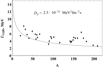
Fig. 1.: Width of the isoscalar GQR versus the nuclear mass number $A$.  The results are obtained from Eqs.  (17) and (16) with $D_{p}(p_{\rm F})=D_{p}=2.5\times 10^{-21}$ $\mathrm{MeV}^{2}\,\mathrm{fm}^{-2}\,\mathrm{s}$.  The experimantal data are taken from Ref. [15]

3.1 Multipole deformation of Fermi surface

In order to analyze the dependence of the collision integral $\mathrm{St}\{f\}$ and of the corresponding relaxation time on the multipolarity of a Fermi surface distortion, we consider below a small deviation $\delta f=f-f_{\mathrm{eq}}$ of the distribution function from the equilibrium.  We shall expand this deviation in a series in spherical harmonics such as

$$\delta f=-\frac{\partial f_{\mathrm{eq}}}{\partial\epsilon}\,\sum_{lm}\,\nu_{lm}(\mathbf{r},t)\,Y_{lm}(\Omega_{p}).$$ (15)

Putting this expanded form into the linearized collision integral (13), we obtain the multipole expansion of $\mathrm{St}\{f\},$ which contains all terms of $l$ starting from $l=0$.  This comes as a consequence of the above-used diffusion approximation.  However, the correct expression for the collision integral does not contain the $l=0$ and $l=1$ terms because of the conservations of the number of particles and the momentum in the collisions. With regard for these constraints, expansion (15), and the expression for the collision integral (9) linearized with respect to $\delta f,$ we derive the relaxation time $\tau_{r,l}$ for the $l$-multipole distortion of the Fermi surface:

$${\frac{1}{\tau_{r,l}}}=-\frac{\displaystyle\int{\frac{d\mathbf{p}}{(2\pi\hbar)^{3}}}\,\,\mathrm{St}\{f\}\,Y_{lm}(\Omega_{p})}{\displaystyle\int{\frac{d\mathbf{p}}{(2\pi\hbar)^{3}}}\,\,\delta f\,Y_{lm}(\Omega_{p})}=$$

$$={\frac{D_{p}(p_{\rm F})}{p_{\rm F}^{2}}}\,l\,(l+1),\quad l\geq 2.$$ (16)

As seen from Eq.  (16), the drift term and, thereby, the nuclear mean field $U$ do not contribute to the relaxation time $\tau_{r,l},$ which is only derived by the diffusion on the distorted Fermi surface.

One can also see from Eq.  (16) that the relaxation time $\tau_{r,l}$ decreases, as the multipolarity $l$ of the Fermi-surface deformation increases.  The nuclear fluid dynamics approximation (FLDA) for the isoscalar excitations corresponds to the case where $l=2$ is preferable, see Ref.  [14].  The fast damping of the higher multipolarities of the Fermi surface distortion in Eq.  (16) gives an argument for the applicability of the FLDA to the description of highly collectivized nuclear excitations.

Relation (16) can be used to adjust the diffusion coefficient $D_{p}(p_{\rm F})$ to the nuclear data.  Within the FLDA, the relaxation time $\tau_{r,l=2}$ derive the width $\Gamma_{\mathrm{GQR}}$ of the isoscalar Giant Quadrupole Resonance (GQR), see Ref.  [14].  Namely,

$$\Gamma_{\mathrm{GQR}}=\frac{4\ \epsilon_{\rm F}\ \hbar}{mr_{0}^{2}}\frac{\tau}{1+(\omega_{\rm R}\tau)^{2}}A^{-2/3},$$ (17)

where $\epsilon_{\rm F}$ is the Fermi energy, $r_{0}$ is the mean nucleon-nucleon distance in the nucleus, $\tau\equiv\tau_{r,l=2,}$ and $\omega_{\rm R}$ is the GQR eigenfrequency.  In Figure 1, we show the results of calculations and the comparison with experimental data for the GQR width for the nuclei through the Periodic table of elements.  We have here adopted $\epsilon_{\rm F}=40$ MeV, $r_{0}=1.2$ fm, and the experimental value of the GQR energy $\hbar\omega_{\rm R}=63A^{-1/3}$ MeV.  The relaxation time $\tau$ in Eq. (17) was taken from Eq. (16) with $D_{p}(p_{\rm F})=D_{p}=2.5\times 10^{-21}$ $\mathrm{MeV}^{2}\,\mathrm{fm}^{-2}\,\mathrm{s}$.

As can be seen from Fig. 1, the FLDA provides a quite satisfactory description of the widths $\Gamma_{\mathrm{GQR}},$ where the quadrupole distortions of the Fermi surface are taken into consideration, and the above-mentioned diffuse coefficient $D_{p}(p_{\rm F})$ is used.

We point out a some peculiarity of the nuclear isovector excitations.  The isovector current is not conserved in the neutron-proton collisions [16], and the dipole distortion of the Fermi surface is represented at the collision integral.  Thus, the term $l=1$ gives an additional contribution to the relaxation of collective isovector excitations [2,​ 17,​ 18].

3.2 Particle-hole distortion of Fermi surface

Another possibility for a distortion of the Fermi surface is the initial non-equilibrium particle-hole excitation.  We will restrict ourselves by a nuclear matter, which is homogeneous in the $\mathbf{r}$-space, and assume a spherical Fermi surface of radius $p_{\rm F}$.  The Fermi momentum is derived by the condition for the particle number $A$ within a fixed volume $\mathcal{V}$

$$\int\limits_{0}^{p_{\rm F}}\frac{4\pi\mathcal{V}\mathsf{g}}{(2\pi\hbar)^{3}}\ p^{2}dp=A.$$

The distorted particle distribution $f_{\mathrm{in}}(p,t=0)$ for the particle-hole excitation at the initial time $t=0$ is given by

$$f_{\mathrm{in}}(p,t=0)=$$

$$=\left[1-\theta(p-p_{1}^{\prime})+\theta(p-p_{2}^{\prime})\right]\left[1-\theta(p-p_{\rm F})\right]+$$

$$+\left[1-\theta(p-p_{2})\right]\theta(p-p_{1})\theta(p-p_{\rm F}),$$ (18)

which means the particle located at $p_{1}<p<p_{2}$ and the hole excitation at $p_{1}^{\prime}<p<p_{2}^{\prime}$ for the fixed $p_{1}>p_{\rm F}$ and $p_{2}^{\prime}<p_{\rm F}$, respectively.  Note that the intervals $\Delta p^{\prime}=p_{2}^{\prime}-p_{1}^{\prime}$ and $\Delta p=p_{2}-p_{1}$ should be taken from the conditions

$$\int\limits_{0}^{p_{\rm F}}\frac{4\pi\mathcal{V}\mathsf{g}dp}{(2\pi\hbar)^{3}}p^{2}f_{\mathrm{in}}(p,t=0)=A-1,$$

$$\int\limits_{p_{\rm F}}^{\infty}\frac{4\pi\mathcal{V}\mathsf{g}dp}{(2\pi\hbar)^{3}}p^{2}f_{\mathrm{in}}(p,t=0)=1.$$

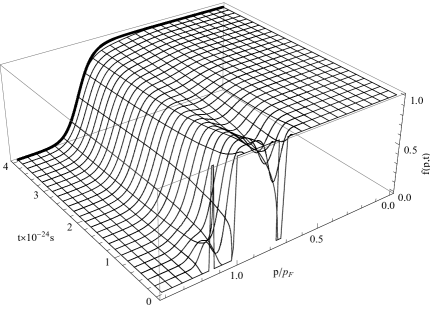
Fig. 2.: Time evolution of the initial distribution function (18) in the momentum space (in units of the Fermi momentum $p_{\rm F}$) with $p_{1}^{\prime}/p_{\rm F}\simeq 0.71$, $p_{2}^{\prime}/p_{\rm F}\simeq 0.75$, $p_{1}/p_{\rm F}\simeq 1.12$, $p_{2}/p_{\rm F}\simeq 1.13$, which corresponds to the initial excitation energy $E_{\mathrm{ex}}=30$  MeV.  The solid line is the Fermi distribution (11) with $T=-D_{p}/K_{p}$. The calculation was performed for $A=16$

Assuming the spherical symmetric distribution, the kinetic equation (10) is rewritten as

$${\frac{\partial f}{\partial t}}=-\frac{K_{p}}{m}\,\left[p\frac{\partial\,}{\partial p}f\,\tilde{f}+3f\,\tilde{f}\ \right]+\frac{D_{p}}{p^{2}}\frac{\partial\,}{\partial p}p^{2}\frac{\partial\,}{\partial p}\,f.$$ (19)

Equation (19) can be solved numerically under the initial condition of Eq. (18).  Below, we will use the transport coefficients $D_{p}=2.5\times 10^{-21}\,\,\mathrm{MeV}^{2}\,\mathrm{fm}^{-2}\,\mathrm{s}$ and $K_{p}=-6.25\times 10^{-22}\,\,\mathrm{MeV}\,\mathrm{fm}^{-2}\,\mathrm{s}$.

In Fig. 2, we have plotted the time evolution of the Wigner distribution function $f(p,t)$ for the initial particle-hole excitation in a nucleus with $A=16$. Here, we have started from the initial distribution $f_{\mathrm{in}}(p,t=0)$ given by Eq.  (18) and have assumed the initial excitation energy $E_{\mathrm{ex}}=30$ MeV.  One can see from Fig. 2 that the momentum distribution $f(p,t)$ evolves to a Fermi-type equilibrium limit $f_{\mathrm{eq}}(p)$ of the sort of Eq. (11).  The corresponding equilibrium temperature of the compound nucleus is obtained as $T=-D_{p}/K_{p}\approx 4\ \mathrm{MeV}$.

Note that the excitation energy $E_{\mathrm{ex}}$ is related to the equilibrium temperature $T$ of the compound nucleus as $E_{\mathrm{ex}}=aT^{2}$, where $a$ is the statistical level density parameter.  In the case under study, we find $a\approx A/8.5$ MeV ^-1.  The obtained value of the level density parameter $a$ agrees with the experimental one $a_{\exp}\simeq A/8$ MeV^-1 [19] quite well.

4 Conclusions

We have considered the equilibration in a many-body Fermi-system caused by the interparticle collision on the distorted Fermi surface.  Our approach combines both the dissipative and diffusive effects providing the time evolution of the system toward the equilibrium limit.  We have discussed two types of non-equilibrium states.  The first one is the multipole deformation of the Fermi surface, which occurs at the sound mode excitation.  We have established that the relaxation time $\tau_{r,l}$ decreases rapidly with the growing multipolarity $l$ of the Fermi-surface distortion. The relaxation time $\tau_{r,l}$ depends here on the diffuse coefficient $D_{p}$ and does not depend on the drift coefficient $K_{p}$.  The second one is the relaxation of the particle-hole excitation.  We have shown that the corresponding relaxation process depends on both transport coefficients $D_{p}$ and $K_{p},$ and the system drifts to the Fermi-type equilibrium limit with the equilibrium temperature $T=-D_{p}/K_{p}$.

В.М. Коломiєць, С.В. Лук’янов
ДИФУЗIЯ НА ДЕФОРМОВАНIЙ ПОВЕРХНI ФЕРМI
Р е з ю м е
Розглянуто наближення дифузiї для опису процесу релаксацiї на збуренiй поверхнi Фермi у фермi-рiдинi. Встановлено залежнiсть часу релаксацiї вiд мультипольностi деформацiї поверхнi Фермi. Дослiджено часову еволюцiю нерiвноважних збуджень частинка–дiрка.

References

- [1] G. Bertsch, Nucl. Phys. A 249, 253 (1975).
- [2] V.M. Kolomietz and H.H.K. Tang, Phys. Scripta 24, 915 (1981).
- [3] G. Eckart, G. Holzwarth, and J.P. da Providencia, Nucl. Phys. A 364, 1 (1981).
- [4] V.M. Kolomietz, Sov. J. Nucl. Phys. 37, 325 (1983).
- [5] A.G. Magner, V.M. Kolomietz, H. Hofmann, and S. Shlomo, Phys. Rev. C 51, 2457 (1995).
- [6] D. Kiderlen, V.M. Kolomietz, and S. Shlomo, Nucl. Phys. A 608, 32 (1996).
- [7] G. Bertsch, Z. Phys. A 289, 103 (1978).
- [8] V.M. Kolomietz, V.A. Plujko, and S. Shlomo, Phys. Rev. C 54, 3014 (1996).
- [9] E.M. Lifshitz and L.P. Pitaevskii, Physical Kinetics (Pergamon Press, Oxford, 1981), Ch. 2.
- [10] L.P. Kadanoff and G. Baym, Quantum Statistical Mechanics (Benjamin, London, 1962), Ch. 9.
- [11] A.A. Abrikosov and I.M. Khalatnikov, Rep. Progr. Phys. 22, 329 (1959).
- [12] P. Ring and P. Schuck, The Nuclear Many-Body Problem (Springer, New York, 1980), Ch. 13.
- [13] G. Wolshin, Phys. Rev. Lett. 48, 1004 (1982).
- [14] V.M. Kolomietz and S. Shlomo, Phys. Rep. 690, 133 (2004).
- [15] F.E. Bertrand, Nucl. Phys. A 354, 129 (1981).
- [16] K. Ando, A. Ikeda, and G. Holzwarth, Z. Phys. A 310, 223 (1983).
- [17] Cai Yanhuang and M. Di Toro, Phys. Rev. C 39, 105 (1989).
- [18] M. Di Toro, V.M. Kolomietz, and A.B. Larionov, Phys. Rev. C 59, 3099 (1999).
-
[19]
S. Shlomo and V.M. Kolomietz, Rep. Prog. Phys. 68, 1 (2005).
Received 15.01.14