Kernel Oriented Generator Distribution

Abstract: Matrix variate beta (MVB) distributions are used in different fields of hypothesis testing, multivariate correlation analysis, zero regression, canonical correlation analysis and etc. In this approach a unified methodology is proposed to generate matrix variate distributions by combining the kernel of MVB distributions of different types with an unknown Borel measurable function of trace operator over matrix space, called generator component. The latter component is a principal element of these newly defined generator type matrix variate distributions. The matrix variate Kummer beta distribution is amongst others a special case. Several statistical properties of this newly defined family of distributions are derived. In the conclusion other extensions and developments are discussed.

Key words and phrases: eigenvalues; generator; invariant polynomials; kernel; moment generating function; Taylor’s series expansion; Zonal polynomial.

AMS Classification: Primary: 62H10, Secondary: 62H15

1 Introduction

It is well-documented that change to the stucture of a known statistical distribution generates a new mutated distribution which performs better in some cases. One interesting and well-known approach is to incorporate the kernel of a statistical distribution to propose another one. Examples include the works of, but not restricted to, Jones (2004), Nadarajah and Kotz (2004, 2006), Brown et al. (2002), Pauw et al. (2010), Silva et al. (2010), Singla et al. (2012) and Ferreira et al. (2012). The weighted distribution is nothing but a mathematical construct to the statistical distribution where there is usually an underlying ‘chance mechanism’ associated with the population of interest (e.g. Nanda and Jain, 1999; Navarro et al., 2006; Kwam, 2008 and Sunoj and Linu, 2012).

In this paper the authors propose a new kernel-generator definition that is a composition of a kernel of a statistical distribution combined with a Borel measurable function of trace operator over matrix space. The kernel oriented generator approach, from matrix variate viewpoint, is defined as follows:

Definition 1.1.

The random symmetric matrix $\bm{X}$ has kernel oriented distribution if it can be represented as

$$f(\bm{X})=C_{o}f^{*}(\bm{X})h(\mathop{\mathrm{t}r}\nolimits\bm{\Phi}\bm{X}),\quad\bm{X}>\bm{0},$$

where $f^{*}(.)$ is the kernel of any statistical distribution, $h(.)$ is a Borel measurable function which admits Taylor’s series expansion, $\bm{\Phi}>\bm{0}$ is the canonical parameter and $C_{o}$ is the normalizing constant.

We turn the reader’s attention to the following:

1. Note: call $f^{\ast}(.)$ and $h(.)$ as the naïve kernel (NK) and principal kernel (PK), respectively.  The latter is also called the generator.

2. It would of major task to find the normalizing constant $C_{o}$, since the PK component can be any function. Recall that an elliptically contoured distribution (even matrix variate form) is a distribution whose characteristic function (density if exists) can be presented as a function of quadratic forms. Thus there is a similarity for the constant $C_{o}$ in the literature. However, we will address the solution to obtain $C_{o}$ by applying the Taylor’s series expansion under some mild regularity conditions.

3. It is thus possible to extend each statistical distribution by taking its NK component and compose it with an extra PK element, which gives an infinity class of distributions. The latter element has many statistical features where the shape of $f(.)$ is the important one. This approach is not restricted to matrix variate distributions only, however some univariate examples are also considered here.

Using Definition 1.1 in this paper, we focus on well-known matrix variate beta kernels. The resulting new distributions will be referred to as matrix variate beta kernel oriented generator distributions or matrix variate beta type 1/2/3 generator distribution (MBG1/2/3) for short.

We organize the paper as follows: In section 2 the definitions of  the matrix variate beta generator distributions of type I, II and III are given. Section 3 is devoted to some important statistical properties of these new distributions, followed by a discussion section. The expressions are given in terms of zonal polynomials, homogeneous invariant polynomials with two or more matrix arguments, Meijer’s G function. The reader is referred to the papers of (Chikuse, 1980; Davis, 1979, 1980 and James, 1961, 1964).

2 Matrix Variate Beta Generator Distributions

The well-known matrix variate beta distributions (Olkin and Rubin, 1962), used in different fields of hypothesis testing, multivariate correlation analysis, zero regression, have been extended by several authors. The matrix variate beta type 3 distribution has been defined, and some of its properties have been studied by Gupta and Nagar (2000b, 2009). More recently Nagar et al. (2013), by using extended matrix variate beta function, generalized the well-known matrix beta type 1 distribution. Gupta and Nagar (2006) extended the work of Nadarajah and Kotz (2006) by defining matrix variate hypergeometric beta distribution. Ehlers (2011) proposed the matrix variate beta type 5 distribution motivating from generalized hypothesis testing in multivariate setup (see also Bekker et al., 2012).

Let $\bm{X}$ be a random symmetric matrix of dimension $m$ and $\mathop{\mathrm{R}e}\nolimits(a),\mathop{\mathrm{R}e}\nolimits(b)>(m-1)/2$. According to Definition 1.1, in this section we define

1. matrix variate beta type 1 generator distribution (MBG1), by taking the NK to be

   $$\det(\bm{X})^{a-\frac{1}{2}(m+1)}\det(\bm{I}-\bm{X})^{b-\frac{1}{2}(m+1)}$$

2. matrix variate beta type 2 generator distribution (MBG2), by taking the NK to be

   $$\det(\bm{X})^{a-\frac{1}{2}(m+1)}\det(\bm{I}+\bm{X})^{-(a+b)}$$

3. matrix variate beta type 3 generator distribution (MBG3), by taking the NK to be

   $$\det(\bm{X})^{a-\frac{1}{2}(m+1)}\det(\bm{I}-\bm{X})^{b-\frac{1}{2}(m+1)}\det(\bm{I}+\bm{X})^{-(a+b)}$$

Further we consider some special cases.

Definition 2.2.

The random symmetric matrix $\bm{X}$ of dimension $m$ is said to have

1. MBG1 distribution with parameters $a$, $b$ and $\bm{\Phi}$ and shape generator $h$, denoted by $\bm{X}\sim MBG1_{m}(a,b,h,\bm{\Phi})$, if it has the following density function

   $$f(\bm{X})=\zeta_{a,b}^{(1)}\det(\bm{X})^{a-\frac{1}{2}(m+1)}\det(\bm{I}_{m}-\bm{X})^{b-\frac{1}{2}(m+1)}h(\mathop{\mathrm{t}r}\nolimits(\bm{\Phi}\bm{X})),\quad\bm{X}\in\mathcal{I}_{m},$$

2. MBG2 distribution with parameters $a$, $b$ and $\bm{\Phi}$ and shape generator $h$, denoted by $\bm{X}\sim MBG2_{m}(a,b,h,\bm{\Phi})$, if it has the following density function

   $$f(\bm{X})=\zeta_{a,b}^{(2)}\det(\bm{X})^{a-\frac{1}{2}(m+1)}\det(\bm{I}_{m}+\bm{X})^{-(a+b)}h(\mathop{\mathrm{t}r}\nolimits(\bm{\Phi}\bm{X})),\quad\bm{X}\in\mathcal{S}_{m},$$

3. MBG3 distribution with parameters $a$, $b$ and $\bm{\Phi}$ and shape generator $h$, denoted by $\bm{X}\sim MBG3_{m}(a,b,h,\bm{\Phi})$, if it has the following density function

   $$f(\bm{X})=\zeta_{a,b}^{(3)}\det(\bm{X})^{a-\frac{1}{2}(m+1)}\det(\bm{I}_{m}-\bm{X})^{b-\frac{1}{2}(m+1)}\det(\bm{I}_{m}+\bm{X})^{-(a+b)}h(\mathop{\mathrm{t}r}\nolimits(\bm{\Phi}\bm{X})),\quad\bm{X}\in\mathcal{I}_{m},$$

where, $\mathcal{S}_{m}$ is the space of all positive definite matrices of order $m$, $\mathcal{I}_{m}$ is the space of all square matrices of order $m$ such that $\bm{I}_{m}-\bm{X}\in\mathcal{S}_{m}$ iff $\bm{X}\in\mathcal{S}_{m}$, and $\mathop{\mathrm{R}e}\nolimits(a)>(m-1)/2$, $\mathop{\mathrm{R}e}\nolimits(b)>(m-1)/2$, $\bm{\Phi}$ is a symmetric complex matrix, $h(.)$ is a Borel measurable function that admits a Taylor’s series expansion and $\zeta_{a,b}^{(j)}$, $j=1,2,3$ are the normalizing constants.

Remark 1.

To find the normalizing constants in Definition 2.2, first we use the Taylor’s series expansion to get

$$h(\mathop{\mathrm{t}r}\nolimits\bm{\Phi}\bm{X})=\sum_{t=0}^{\infty}\frac{h^{(t)}(0)}{t!}\;\mathop{\mathrm{t}r}\nolimits(\bm{\Phi}\bm{X})^{t}=\sum_{t=0}^{\infty}\frac{h^{(t)}(0)}{t!}\sum_{\tau}C_{\tau}(\bm{\Phi}\bm{X}),$$ (1)

where $C_{\tau}(.)$ is the zonal polynomial, and we used ordered partitions in use of the zonal polynomials. Then $\zeta_{a,b}^{(j)}$, $j=1,2,3$ can be obtained after some matrix algebra as:

$$\left(\zeta_{a,b}^{(1)}\right)^{-1} = \sum_{t=0}^{\infty}\frac{h^{(t)}(0)}{t!}\sum_{\tau}\int_{\mathcal{I}_{m}}\det(\bm{X})^{a-\frac{1}{2}(m+1)}\det(\bm{I}_{m}-\bm{X})^{b-\frac{1}{2}(m+1)}C_{\tau}(\bm{\Phi}\bm{X})\textnormal{d}\bm{X}$$

$$= \sum_{t=0}^{\infty}\frac{h^{(t)}(0)}{t!}\sum_{\tau}\frac{\Gamma_{m}(a,\tau)\Gamma_{m}(b)}{\Gamma_{m}(a+b,\tau)}C_{\tau}(\bm{\Phi}),\quad\mbox{Theorem 7.2.10\;of\;Muirhead\;(2005)}$$

$$\left(\zeta_{a,b}^{(2)}\right)^{-1} = \sum_{t=0}^{\infty}\frac{h^{(t)}(0)}{t!}\sum_{\tau}\int_{\mathcal{S}_{m}}\det(\bm{X})^{a-\frac{1}{2}(m+1)}\det(\bm{I}_{m}+\bm{X})^{-(a+b)}C_{\tau}(\bm{\Phi}\bm{X})\textnormal{d}\bm{X}$$

$$= \sum_{t=0}^{\infty}\frac{h^{(t)}(0)}{t!}\sum_{\tau}\frac{\Gamma_{m}(a,\tau)\Gamma_{m}(b,-\tau)}{\Gamma_{m}(a+b)}C_{\tau}(\bm{\Phi}),\quad\mbox{Lemma 5\;of\;Khatri\;(1966)}$$

$$\left(\zeta_{a,b}^{(3)}\right)^{-1} = \sum_{t=0}^{\infty}\frac{h^{(t)}(0)}{t!}\sum_{\tau}\int_{\mathcal{I}_{m}}\det(\bm{X})^{a-\frac{1}{2}(m+1)}\det(\bm{I}_{m}-\bm{X})^{b-\frac{1}{2}(m+1)}\det(\bm{I}_{m}+\bm{X})^{-(a+b)}C_{\tau}(\bm{\Phi}\bm{X})\textnormal{d}\bm{X}$$

$$= \sum_{t=0}^{\infty}\frac{h^{(t)}(0)}{t!}\sum_{\tau}\sum_{k=0}^{\infty}\sum_{\kappa}\frac{(-1)^{k}(a+b)_{\kappa}}{k!}$$

$$\int_{\mathcal{I}_{m}}\det(\bm{X})^{a-\frac{1}{2}(m+1)}\det(\bm{I}_{m}-\bm{X})^{b-\frac{1}{2}(m+1)}C_{\kappa}(\bm{X})C_{\tau}(\bm{\Phi}\bm{X})\textnormal{d}\bm{X}\quad$$

$$= \sum_{t=0}^{\infty}\frac{h^{(t)}(0)}{t!}\sum_{\tau}\sum_{k=0}^{\infty}\sum_{\kappa}\frac{(-1)^{k}(a+b)_{\kappa}}{k!}\sum_{\phi\in\kappa\cdot\tau}\theta_{\phi}^{\kappa,\tau}$$

$$\int_{\mathcal{I}_{m}}\det(\bm{X})^{a-\frac{1}{2}(m+1)}\det(\bm{I}_{m}-\bm{X})^{b-\frac{1}{2}(m+1)}C_{\phi}^{\kappa,\tau}(\bm{X},\bm{\Phi}\bm{X})\textnormal{d}\bm{X},\quad\mbox{Eq. (2.8)\; of\; Davis\;(1979)}$$

$$= \sum_{t=0}^{\infty}\frac{h^{(t)}(0)}{t!}\sum_{\tau}\sum_{k=0}^{\infty}\sum_{\kappa}\frac{(-1)^{k}(a+b)_{\kappa}}{k!}\sum_{\phi\in\kappa\cdot\tau}\theta_{\phi}^{\kappa,\tau}$$

$$\frac{\Gamma_{m}(b)\Gamma_{m}(a,\phi)}{\Gamma_{m}(a+b,\phi)}C_{\phi}^{\kappa,\tau}(\bm{I}_{m},\bm{\Phi}),\quad\mbox{Eq. (3.28)\; of\; Chikuse\;(1980)}$$

$$= \sum_{\tau,\kappa,\phi}\frac{(-1)^{k}(a+b)_{\kappa}h^{(t)}(0)}{t!k!}\frac{\Gamma_{m}(b)\Gamma_{m}(a,\phi)}{\Gamma_{m}(a+b,\phi)}\frac{\left(\theta_{\phi}^{\kappa,\tau}\right)^{2}C_{\phi}(\bm{I}_{m})}{C_{\tau}(\bm{I}_{m})}C_{\tau}(\bm{\Phi}),$$

$$\qquad\qquad\qquad\qquad\qquad\qquad\qquad\qquad\qquad\qquad\qquad\qquad\mbox{Eq. (2.2)\; of\; Davis\;(1979)},$$

where $\theta_{\phi}^{\kappa,\tau}=C_{\phi}^{\kappa,\tau}(\bm{I}_{m},\bm{I}_{m})/C_{\phi}(\bm{I}_{m})$, $\sum_{\tau,\kappa,\phi}\equiv\sum_{t=0}^{\infty}\sum_{k=0}^{\infty}\sum_{\tau}\sum_{\kappa}\sum_{\phi\in\kappa\cdot\tau}$, $\Gamma_{p}(.)$ represents the multivariate gamma function, and $\Gamma_{p}(.,\kappa)$ the generalized gamma function of weight $\kappa$. (See Gupta and Nagar, 2000a)

3 Characteristics

In this section we provide some important statistical properties for three different types of matrix variate beta generator distributions.

The following result is straightforward.

Theorem 3.1.

Let $\bm{X}_{i}\sim MBGi_{m}(a,b,h,\bm{\Phi})$, $i=1,2,3$. Then it follows that

$$E\left(\det(\bm{X}_{1})^{r}\right) = \zeta_{a,b}^{(1)}\sum_{t=0}^{\infty}\frac{h^{(t)}(0)}{t!}\sum_{\tau}\frac{\Gamma_{m}(a+r,\tau)\Gamma_{m}(b)}{\Gamma_{m}(a+r+b,\tau)}C_{\tau}(\bm{\Phi}),$$

$$E\left(\det(\bm{X}_{2})^{r}\right) = \zeta_{a,b}^{(2)}\sum_{t=0}^{\infty}\frac{h^{(t)}(0)}{t!}\sum_{\tau}\frac{\Gamma_{m}(a+r,\tau)\Gamma_{m}(b,-\tau)}{\Gamma_{m}(a+r+b)}C_{\tau}(\bm{\Phi}),$$

$$E\left(\det(\bm{X}_{3})^{r}\right) = \zeta_{a,b}^{(3)}\sum_{\tau,\kappa,\phi}\frac{(-1)^{k}(a+b)_{\kappa}h^{(t)}(0)}{t!k!}\frac{\Gamma_{m}(a+r,\phi)\Gamma_{m}(b)}{\Gamma_{m}(a+b+r,\phi)}\frac{\left(\theta_{\phi}^{\kappa,\tau}\right)^{2}C_{\phi}(\bm{I}_{m})}{C_{\tau}(\bm{I}_{m})}C_{\tau}(\bm{\Phi})$$

In the following theorem, we give the moment generating function (MGF) for each type of MBG distribution.

Theorem 3.2.

Denote the MGF of $\bm{X}_{i}\sim MBGi_{m}(a,b,h,\bm{\Phi})$, $i=1,2,3$ by $\mathcal{M}_{i}$. Then we have

$$\mathcal{M}_{1}(\bm{T}) = \zeta_{a,b}^{(1)}\sum_{\tau,\kappa,\phi}\frac{h^{(t)}(0)}{t!k!}\theta_{\phi}^{\kappa,\tau}\frac{\Gamma_{m}(a,\phi)\Gamma_{m}(b)}{\Gamma_{m}(a+b,\phi)}C_{\phi}^{\kappa,\tau}(\bm{T},\bm{\Phi}),$$

$$\mathcal{M}_{2}(\bm{T}) = \zeta_{a,b}^{(2)}\det(\bm{T})^{-a}\sum_{\tau,\kappa,\phi}\frac{h^{(t)}(0)}{t!}\frac{(-1)^{-(am+t)}(a+b)_{\kappa}}{k!}\theta_{\phi}^{\kappa,\tau}\Gamma_{m}(a,\phi)C_{\phi}(\bm{T}^{-1},\bm{T}^{-1}\bm{\Phi}),$$

$$\mathcal{M}_{3}(\bm{T}) = \zeta_{a,b}^{(3)}\sum_{\tau,\kappa,\lambda,\phi}\frac{h^{(t)}(0)}{t!k!}\frac{(-1)^{l}(a+b)_{\lambda}}{l!}\theta_{\phi}^{\kappa,\tau,\lambda}\frac{\Gamma_{m}(a,\phi)\Gamma_{m}(b)}{\Gamma_{m}(a+b,\phi)}C_{\phi}^{\kappa,\tau,\lambda}(\bm{T},\bm{\Phi},\bm{I}),$$

where $\sum_{\tau,\kappa,\lambda,\phi}\equiv\sum_{t=0}^{\infty}\sum_{\tau}\sum_{k=0}^{\infty}\sum_{\kappa}\sum_{l=0}^{\infty}\sum_{\lambda}\sum_{\phi\in\kappa\cdot\tau\cdot\lambda}$ and $\theta_{\phi}^{\kappa,\tau,\lambda}=C_{\phi}^{\kappa,\tau,\lambda}(\bm{I}_{m},\bm{I}_{m},\bm{I}_{m})/C_{\phi}(\bm{I}_{m})$.

Proof: The proof of $\mathcal{M}_{1}$ is straightforward. Here we provide the proofs of $\mathcal{M}_{2}$ & $\mathcal{M}_{3}$.

Using Taylor’s series expansion for $h$, and Eq. (3.10) of Chikuse (1980) we get

$$\mathcal{M}_{2}(\bm{T}) = \zeta_{a,b}^{(2)}\int_{\mathcal{S}_{m}}\det(\bm{X})^{a-\frac{1}{2}(m+1)}\det(\bm{I}_{m}+\bm{X})^{-(a+b)}$$

$$h(\mathop{\mathrm{t}r}\nolimits(\bm{\Phi}\bm{X}))\mathop{\mathrm{e}tr}\nolimits(\bm{T}\bm{X})\mathnormal{d}\bm{X}$$

$$= \zeta_{a,b}^{(2)}\sum_{t=0}^{\infty}\sum_{\tau}\sum_{k=0}^{\infty}\sum_{\kappa}\frac{h^{(t)}(0)}{t!}\frac{(-1)^{k}(a+b)_{\kappa}}{k!}$$

$$\int_{\mathcal{S}_{m}}\det(\bm{X})^{a-\frac{1}{2}(m+1)}C_{\tau}(\bm{\Phi}\bm{X})C_{\kappa}(\bm{X})\mathop{\mathrm{e}tr}\nolimits(\bm{T}\bm{X})\mathnormal{d}\bm{X}$$

$$= \zeta_{a,b}^{(2)}\sum_{t=0}^{\infty}\sum_{\tau}\sum_{k=0}^{\infty}\sum_{\kappa}\frac{h^{(t)}(0)}{t!}\frac{(-1)^{k}(a+b)_{\kappa}}{k!}\sum_{\phi\in\kappa\cdot\tau}\theta_{\phi}^{\kappa,\tau}$$

$$\int_{\mathcal{S}_{m}}\det(\bm{X})^{a-\frac{1}{2}(m+1)}C_{\phi}^{\kappa,\tau}(\bm{X},\bm{\Phi}\bm{X})\mathop{\mathrm{e}tr}\nolimits(\bm{T}\bm{X})\mathnormal{d}\bm{X}.$$

Using Eq. (3.21) of Chikuse (1980) we obtain

$$\mathcal{M}_{2}(\bm{T}) = \zeta_{a,b}^{(2)}\sum_{t=0}^{\infty}\sum_{\tau}\sum_{k=0}^{\infty}\sum_{\kappa}\frac{h^{(t)}(0)}{t!}\frac{(-1)^{k}(a+b)_{\kappa}}{k!}\sum_{\phi\in\kappa\cdot\tau}\theta_{\phi}^{\kappa,\tau}$$

$$\Gamma_{m}(a,\phi)(-1)^{-(am+t+k)}\det(\bm{T})^{-a}C_{\phi}(\bm{T}^{-1},\bm{T}^{-1}\bm{\Phi}).$$

For the MGF of MBG3, by making use of Taylor’s series expansion for $h$, and Eq. (3.10) of Chikuse (1980) we get

$$\mathcal{M}_{3}(\bm{T}) = \zeta_{a,b}^{(3)}\int_{\mathcal{I}_{m}}\det(\bm{X})^{a-\frac{1}{2}(m+1)}\det(\bm{I}_{m}-\bm{X})^{b-\frac{1}{2}(m+1)}\det(\bm{I}_{m}+\bm{X})^{-(a+b)}$$

$$h(\mathop{\mathrm{t}r}\nolimits(\bm{\Phi}\bm{X}))\mathop{\mathrm{e}tr}\nolimits(\bm{T}\bm{X})\mathnormal{d}\bm{X}$$

$$= \zeta_{a,b}^{(3)}\sum_{t=0}^{\infty}\sum_{\tau}\sum_{k=0}^{\infty}\sum_{\kappa}\frac{h^{(t)}(0)}{t!k!}\sum_{l=0}^{\infty}\sum_{\lambda}\frac{(-1)^{l}(a+b)_{\lambda}}{l!}$$

$$\int_{\mathcal{I}_{m}}\det(\bm{X})^{a-\frac{1}{2}(m+1)}\det(\bm{I}_{m}-\bm{X})^{b-\frac{1}{2}(m+1)}C_{\tau}(\bm{\Phi}\bm{X})C_{\kappa}(\bm{T}\bm{X})C_{\lambda}(\bm{X})\mathnormal{d}\bm{X}$$

$$= \zeta_{a,b}^{(3)}\sum_{t=0}^{\infty}\sum_{\tau}\sum_{k=0}^{\infty}\sum_{\kappa}\frac{h^{(t)}(0)}{t!k!}\sum_{l=0}^{\infty}\sum_{\lambda}\frac{(-1)^{l}(a+b)_{\lambda}}{l!}\sum_{\phi\in\kappa\cdot\tau\cdot\lambda}\theta_{\phi}^{\kappa,\tau,\lambda}$$

$$\int_{\mathcal{I}_{m}}\det(\bm{X})^{a-\frac{1}{2}(m+1)}\det(\bm{I}_{m}-\bm{X})^{b-\frac{1}{2}(m+1)}C_{\phi}^{\kappa,\tau,\lambda}(\bm{T}\bm{X},\bm{\Phi}\bm{X},\bm{X})\mathnormal{d}\bm{X}.$$

Finally applying Eq. (3.28) of Chikuse (1980), yields

$$\mathcal{M}_{3}(\bm{T}) = \zeta_{a,b}^{(3)}\sum_{t=0}^{\infty}\sum_{\tau}\sum_{k=0}^{\infty}\sum_{\kappa}\frac{h^{(t)}(0)}{t!k!}\sum_{l=0}^{\infty}\sum_{\lambda}\frac{(-1)^{l}(a+b)_{\lambda}}{l!}$$

$$\sum_{\phi\in\kappa\cdot\tau\cdot\lambda}\theta_{\phi}^{\kappa,\tau,\lambda}\frac{\Gamma_{m}(a,\phi)\Gamma_{m}(b)}{\Gamma_{m}(a+b,\phi)}C_{\phi}^{\kappa,\tau,\lambda}(\bm{T},\bm{\Phi},\bm{I}).$$

and the proof is complete. $\blacksquare$

In the following result, we give the exact expressions for the cumulative distribution function (CDF) of MBG1/2/3 distribution.

Theorem 3.3.

Denote the CDF of $\bm{X}_{i}\sim MBGi_{m}(a,b,h,\bm{\Phi})$, $i=1,2,3$ by $F_{i}$. Then we have

$$F_{1}(\bm{Y}) = \zeta_{a,b}^{(1)}\det(\bm{Y})^{a}\sum_{\tau,\kappa,\phi}\frac{\left(-b+\frac{1}{2}(m+1)\right)_{\kappa}}{k!}\frac{h^{(t)}(0)}{t!}\frac{\Gamma_{m}(a,\phi)\Gamma\left(\frac{m+1}{2}\right)}{\Gamma\left(a+\frac{m+1}{2},\phi\right)}$$

$$\times\theta_{\phi}^{\kappa,\tau}C_{\phi}^{\kappa,\tau}(\bm{Y},\bm{Y}^{\frac{1}{2}}\bm{\Phi}\bm{Y}^{\frac{1}{2}}),$$

$$F_{2}(\bm{Y}) = \zeta_{a,b}^{(2)}\det(\bm{Y})^{a}\sum_{\tau,\kappa,\phi}\frac{(-1)^{k}\left(a+b\right)_{\kappa}}{k!}\frac{h^{(t)}(0)}{t!}\frac{\Gamma_{m}(a,\phi)\Gamma\left(\frac{m+1}{2}\right)}{\Gamma\left(a+\frac{m+1}{2},\phi\right)}$$

$$\times\theta_{\phi}^{\kappa,\tau}C_{\phi}^{\kappa,\tau}(\bm{Y},\bm{Y}^{\frac{1}{2}}\bm{\Phi}\bm{Y}^{\frac{1}{2}}),$$

$$F_{3}(\bm{Y}) = \zeta_{a,b}^{(3)}\det(\bm{Y})^{a}\sum_{\kappa,\tau,\lambda,\phi}\frac{\left(-b+\frac{1}{2}(m+1)\right)_{\kappa}}{k!}\frac{h^{(t)}(0)}{t!}\frac{(-1)^{l}(a+b)_{\lambda}}{l!}\frac{\Gamma_{m}\left(\frac{m+1}{2}\right)\Gamma_{m}(a,\phi)}{\Gamma_{m}\left(a+\frac{m+1}{2},\phi\right)}$$

$$\times\theta_{\phi}^{\kappa,\tau,\lambda}C_{\phi}^{\kappa,\tau,\lambda}(\bm{Y},\bm{Y}^{\frac{1}{2}}\bm{\Phi}\bm{Y}^{\frac{1}{2}},\bm{Y})$$

Proof: For the CDF of MBG1 distribution, we have by definition

$$F_{1}(\bm{Y})=\zeta_{a,b}^{(1)}\int_{0<\bm{X}<\bm{Y}<\bm{I}_{m}}\det(\bm{X})^{a-\frac{1}{2}(m+1)}\det(\bm{I}_{m}-\bm{X})^{b-\frac{1}{2}(m+1)}h(\mathop{\mathrm{t}r}\nolimits(\bm{\Phi}\bm{X}))\mathnormal{d}\bm{X}.$$

Making the transformation $\bm{G}=\bm{Y}^{-\frac{1}{2}}\bm{X}\bm{Y}^{-\frac{1}{2}}$ with the Jacobian $J(\bm{X}\rightarrow\bm{G})=\det(\bm{Y})^{\frac{1}{2}(m+1)}$ we get

$$F_{1}(\bm{Y}) = \zeta_{a,b}^{(1)}\det(\bm{Y})^{a}\int_{\mathcal{I}_{m}}\det(\bm{G})^{a-\frac{1}{2}(m+1)}\det(\bm{I}_{p}-\bm{Y}^{\frac{1}{2}}\bm{G}\bm{Y}^{\frac{1}{2}})^{b-\frac{1}{2}(m+1)}$$

$$\times h\left(\mathop{\mathrm{t}r}\nolimits(\bm{\Phi}\bm{Y}^{\frac{1}{2}}\bm{G}\bm{Y}^{\frac{1}{2}})\right)\mathnormal{d}\bm{G}$$

$$= \zeta_{a,b}^{(1)}\det(\bm{Y})^{a}\sum_{k=0}^{\infty}\sum_{\kappa}\frac{\left(-b+\frac{1}{2}(m+1)\right)_{\kappa}}{k!}\int_{\mathcal{I}_{m}}\det(\bm{G})^{a-\frac{1}{2}(m+1)}$$

$$\times C_{\kappa}(\bm{Y}^{\frac{1}{2}}\bm{G}\bm{Y}^{\frac{1}{2}})h\left(\mathop{\mathrm{t}r}\nolimits(\bm{\Phi}\bm{Y}^{\frac{1}{2}}\bm{G}\bm{Y}^{\frac{1}{2}})\right)\mathnormal{d}\bm{G}.$$

Make use of Taylor’s series expansion for $h(.)$ term and equations (3.10) and (3.32) of Chikuse (1980) to obtain

$$F_{1}(\bm{Y}) = \zeta_{a,b}^{(1)}\det(\bm{Y})^{a}\sum_{k=0}^{\infty}\sum_{\kappa}\frac{\left(-b+\frac{1}{2}(m+1)\right)_{\kappa}}{k!}\sum_{t=0}^{\infty}\frac{h^{(t)}(0)}{t!}\sum_{\tau}$$

$$\times\int_{\mathcal{I}_{m}}\det(\bm{G})^{a-\frac{1}{2}(m+1)}C_{\phi}^{\kappa,\tau}(\bm{Y}\bm{G},\bm{Y}^{\frac{1}{2}}\bm{\Phi}\bm{Y}^{\frac{1}{2}}\bm{G})\mathnormal{d}\bm{G}$$

$$= \zeta_{a,b}^{(1)}\det(\bm{Y})^{a}\sum_{k=0}^{\infty}\sum_{\kappa}\frac{\left(-b+\frac{1}{2}(m+1)\right)_{\kappa}}{k!}\sum_{t=0}^{\infty}\frac{h^{(t)}(0)}{t!}\sum_{\tau}\sum_{\phi\in\kappa\cdot\tau}\theta_{\phi}^{\kappa,\tau}$$

$$\times\frac{\Gamma_{m}(a,\phi)\Gamma_{m}\left(\frac{1}{2}(m+1)\right)}{\Gamma_{m}\left(a+\frac{1}{2}(m+1),\phi\right)}C_{\phi}^{\kappa,\tau}(\bm{Y},\bm{Y}^{\frac{1}{2}}\bm{\Phi}\bm{Y}^{\frac{1}{2}}).$$

The CDF of MBG2 distribution can be obtained in the same fashion as for the CDF of MBG1 distribution. For the CDF of MBG3 distribution, using the same procedure as in the proof of the CDF of MBG1 distribution, we have

$$F_{3}(\bm{Y}) = \zeta_{a,b}^{(3)}\det(\bm{Y})^{a}\sum_{k=0}^{\infty}\sum_{\kappa}\frac{\left(-b+\frac{1}{2}(m+1)\right)_{\kappa}}{k!}\sum_{t=0}^{\infty}\frac{h^{(t)}(0)}{t!}\sum_{\tau}\sum_{l=0}^{\infty}\sum_{\lambda}\frac{(-1)^{l}(a+b)_{\lambda}}{l!}$$

$$\times\int_{\mathcal{I}_{m}}\det(\bm{G})^{a-\frac{1}{2}(m+1)}C_{\kappa}(\bm{Y}\bm{G})C_{\tau}(\bm{Y}^{\frac{1}{2}}\bm{\Phi}\bm{Y}^{\frac{1}{2}}\bm{G})C_{\lambda}(\bm{Y}\bm{G})\mathnormal{d}\bm{G}$$

$$= \zeta_{a,b}^{(3)}\det(\bm{Y})^{a}\sum_{k=0}^{\infty}\sum_{\kappa}\frac{\left(-b+\frac{1}{2}(m+1)\right)_{\kappa}}{k!}\sum_{t=0}^{\infty}\frac{h^{(t)}(0)}{t!}\sum_{\tau}\sum_{l=0}^{\infty}\sum_{\lambda}\frac{(-1)^{l}(a+b)_{\lambda}}{l!}\sum_{\phi\in\kappa\cdot\tau\cdot\lambda}\theta_{\phi}^{\kappa,\tau,\lambda}$$

$$\times\int_{\mathcal{I}_{m}}\det(\bm{G})^{a-\frac{1}{2}(m+1)}C_{\phi}^{\kappa,\tau,\lambda}(\bm{Y}\bm{G},\bm{Y}^{\frac{1}{2}}\bm{\Phi}\bm{Y}^{\frac{1}{2}}\bm{G},\bm{Y}\bm{G})\mathnormal{d}\bm{G},\quad\mbox{Eq.\;(3.10)\;of\;Chikuse\;(1980)}.$$

Make use of Eq. (3.32) of Chikuse (1980) to get

$$F_{3}(\bm{Y}) = \zeta_{a,b}^{(3)}\det(\bm{Y})^{a}\sum_{k=0}^{\infty}\sum_{\kappa}\frac{\left(-b+\frac{1}{2}(m+1)\right)_{\kappa}}{k!}\sum_{t=0}^{\infty}\frac{h^{(t)}(0)}{t!}\sum_{\tau}\sum_{l=0}^{\infty}\sum_{\lambda}\frac{(-1)^{l}(a+b)_{\lambda}}{l!}\sum_{\phi\in\kappa\cdot\tau\cdot\lambda}\theta_{\phi}^{\kappa,\tau,\lambda}$$

$$\times\frac{\Gamma_{m}\left(\frac{m+1}{2}\right)\Gamma_{m}(a,\phi)}{\Gamma_{m}\left(a+\frac{m+1}{2},\phi\right)}C_{\phi}^{\kappa,\tau,\lambda}(\bm{Y},\bm{Y}^{\frac{1}{2}}\bm{\Phi}\bm{Y}^{\frac{1}{2}},\bm{Y})$$

which completes the proof. $\blacksquare$
In what follows, we are interested in the distribution of quadratic forms from MBG distributions. Assume $\bm{\Psi},\bm{\Omega}\in\mathcal{S}_{m}$ are some known matrix parameters and under the meaning of partial löwner ordering, $\bm{\Omega}>\bm{\Psi}$. We are interested in the distribution of the random matrix variate

$$\bm{Y}_{i}=(\bm{\Omega}-\bm{\Psi})^{\frac{1}{2}}\bm{X}_{i}(\bm{\Omega}-\bm{\Psi})^{\frac{1}{2}}+\bm{\Psi},$$ (2)

where $\bm{X}_{i}\sim MBGi_{m}(a,b,h,\bm{\Phi})$, $i=1,2,3$. The distribution of $\bm{Y}_{i}$ is the MBG distribution, which is given in the following result.

Theorem 3.4.

Suppose that $f(\bm{Y}_{i})$ is the density function given by $\eqref{composite}$, while $\bm{X}_{i}\sim MBGi_{m}(a,b,h,\bm{\Phi})$, $i=1,2,3$. Then we have

$$f(\bm{Y}_{1}) = \zeta_{a,b}^{(1)}\det(\bm{Y}_{1}-\bm{\Psi})^{a-\frac{1}{2}(m+1)}\det(\bm{\Omega}-\bm{Y}_{1})^{b-\frac{1}{2}(m+1)}\det(\bm{\Omega}-\bm{\Psi})^{-(a+b)+\frac{1}{2}(m+1)}h(\mathop{\mathrm{t}r}\nolimits\bm{\Theta}(\bm{Y}_{1}-\bm{\Psi})),$$

$$f(\bm{Y}_{2}) = \zeta_{a,b}^{(2)}\det(\bm{Y}_{2}-\bm{\Psi})^{a-\frac{1}{2}(m+1)}\det(\bm{\Omega}+\bm{Y}_{2}-2\bm{\Psi})^{-(a+b)}\det(\bm{\Omega}-\bm{\Psi})^{b}h(\mathop{\mathrm{t}r}\nolimits\bm{\Theta}(\bm{Y}_{2}-\bm{\Psi}))$$

$$f(\bm{Y}_{3}) = \zeta_{a,b}^{(3)}\det(\bm{Y}_{3}-\bm{\Psi})^{a-\frac{1}{2}(m+1)}\det(\bm{\Omega}-\bm{Y}_{3})^{b-\frac{1}{2}(m+1)}\det(\bm{\Omega}+\bm{Y}_{3}-2\bm{\Psi})^{-(a+b)}$$

$$\det(\bm{\Omega}-\bm{\Psi})^{\frac{1}{2}(m+1)}h(\mathop{\mathrm{t}r}\nolimits\bm{\Theta}(\bm{Y}_{3}-\bm{\Psi})),$$

where $\bm{\Psi}<\bm{Y}_{i}<\bm{\Omega}$, $i=1,2,3$ and $\bm{\Theta}=(\bm{\Omega}-\bm{\Psi})^{-\frac{1}{2}}\bm{\Phi}(\bm{\Omega}-\bm{\Psi})^{-\frac{1}{2}}$.

Proof: From Definition 2.2 and the fact that the Jacobian of transformation is $J(\bm{X}\rightarrow\bm{Y})=\det(\bm{\Omega}-\bm{\Psi})^{-\frac{1}{2}(m+1)}$, the result follows. $\blacksquare$.

Remark 2.

Suppose that $\bm{X}_{i}\sim MBGi_{m}(a,b,\bm{\Phi},h)$, $i=1,2,3$ and $\bm{A}$ is a constant $m$-dimensional nonsingular matrix. Then using Theorem 3.4, the linear combination $\bm{A}\bm{X}_{i}\bm{A}^{\prime}$, $i=1,2,3$ has the MBG distribution.

Remark 3.

In Theorem 3.4, it might be seemed that “generalized noncentral” MBG distributions of three types are defined.

Entropy measures the uncertainty as confined in a distribution. Formally let $(\chi,\mathcal{B},\mathcal{P})$ be a probability space, $f(.)$ is a density function of matrix variate $\bm{X}$, associated with $\mathcal{P}$, dominated by the $\sigma$-measure $\mu$ on $\chi$. The Shannon entropy measures the expected information contained in the data and is equivalent to the unpredicted component of a distribution. Then the well-known Shannon entropy of $f$ is defined by

$$E_{S}(f)=-\int_{\chi}f(\bm{X})\log f(\bm{X})\mathnormal{d}\mu.$$

As an extension to the above measure, Rényi entropy is defined as

$$E_{R}(f)=\frac{1}{1-\nu}\log\int_{\chi}f^{\nu}(\bm{X})\mathnormal{d}\mu,\quad\nu>0\ \mbox{and}\ \nu\neq 1.$$

The additional parameter $\nu$, is used to describe complex behavior in probability models and the associated process under study. Rényi entropy monotonically decreasing in $\nu$, while Shannon entropy is obtained from Rényi for $\nu\uparrow 1$. For details see Zagrafos and Nadarajah (2005). The Rényi entropy for these distributions is derived as follows.

Theorem 3.5.

1. Let $\bm{X}\sim MBG1_{m}(a,b,h,\bm{\Phi})$. Then the Rényi entropy is given by

   $$E_{R}(f) = \frac{1}{1-\nu}\log\bigg{[}\left(\zeta_{a,b}^{(1)}\right)^{\nu}\sum_{t=0}^{\infty}\frac{u^{(t)}(0)}{t!}\sum_{\tau}$$

   $$\frac{\Gamma_{m}\left(\nu a-\frac{1}{2}(\nu-1)(m+1),\tau\right)\Gamma_{m}\left(b\nu-\frac{1}{2}(\nu-1)(m+1)\right)}{\Gamma_{m}\left(\nu a+\nu b-(\nu-1)(m+1),\tau\right)}C_{\tau}(\bm{\Phi})\bigg{]},$$

2. Let $\bm{X}\sim MBG2_{m}(a,b,h,\bm{\Phi})$. Then the Rényi entropy is given by

   $$E_{R}(f) = \frac{1}{1-\nu}\log\bigg{[}\left(\zeta_{a,b}^{(2)}\right)^{\nu}\sum_{t=0}^{\infty}\frac{u^{(t)}(0)}{t!}\sum_{\tau}$$

   $$\frac{\Gamma_{m}\left(\nu a-\frac{1}{2}(\nu-1)(m+1),\tau\right)\Gamma_{m}\left(b\nu-\frac{1}{2}(\nu-1)(m+1),-\tau\right)}{\Gamma_{m}\left(\nu a+\nu b-(\nu-1)(m+1)\right)}C_{\tau}(\bm{\Phi})\bigg{]},$$

3. Let $\bm{X}\sim MBG3_{m}(a,b,h,\bm{\Phi})$. Then the Rényi entropy is given by

   $$E_{R}(f) = \frac{1}{1-\nu}\log\bigg{[}\left(\zeta_{a,b}^{(3)}\right)^{\nu}\sum_{\tau,\kappa,\phi}\frac{(-1)^{k}(\nu a+\nu b-(\nu-1)(m+1))_{\kappa}h^{(t)}(0)}{t!k!}$$

   $$\frac{\Gamma_{m}\left(\nu a-\frac{1}{2}(\nu-1)(m+1),\phi\right)\Gamma_{m}\left(b\nu-\frac{1}{2}(\nu-1)(m+1)\right)}{\Gamma_{m}(\nu a+\nu b-(\nu-1)(m+1),\phi)}\frac{\left(\theta_{\phi}^{\kappa,\tau}\right)^{2}C_{\phi}(\bm{I}_{m})}{C_{\tau}(\bm{I}_{m})}C_{\tau}(\bm{\Phi})\bigg{]},$$

where $u^{(t)}$ is the $t$-th derivative of $h^{\nu}$.

Proof: By Definition 2.2, for MBG1 distribution, we have that

$$I(\nu) = \int_{\mathcal{I}_{m}}f^{\nu}(\bm{X})\mathnormal{d}\bm{X}$$

$$= \left(\zeta_{a,b}^{(1)}\right)^{\nu}\int_{\mathcal{I}_{m}}\det(\bm{X})^{\nu a-\frac{1}{2}(\nu-1)(m+1)-\frac{1}{2}(m+1)}\det(\bm{I}_{m}-\bm{X})^{\nu b-\frac{1}{2}(\nu-1)(m+1)-\frac{1}{2}(m+1)}$$

$$\times h^{\nu}(\mathop{\mathrm{t}r}\nolimits(\bm{\Phi}\bm{X}))\mathnormal{d}\bm{X}.$$

Since $u(\mathop{\mathrm{t}r}\nolimits(\bm{\Phi}\bm{X}))=h^{\nu}(\mathop{\mathrm{t}r}\nolimits(\bm{\Phi}\bm{X}))$ is a Borel measurable function that admits a Taylor’s series expansion in zonal polynomials under some mild conditions, we get

$$I(\nu) = \left(\zeta_{a,b}^{(1)}\right)^{\nu}\int_{\mathcal{I}_{m}}\det(\bm{X})^{\nu a-\frac{1}{2}(\nu-1)(m+1)-\frac{1}{2}(m+1)}\det(\bm{I}_{m}-\bm{X})^{\nu b-\frac{1}{2}(\nu-1)(m+1)-\frac{1}{2}(m+1)}$$

$$\times u(\mathop{\mathrm{t}r}\nolimits(\bm{\Phi}\bm{X}))\mathnormal{d}\bm{X}$$

$$= \left(\zeta_{a,b}^{(1)}\right)^{\nu}\sum_{t=0}^{\infty}\frac{u^{(t)}(0)}{t!}\sum_{\tau}\frac{\Gamma_{m}\left(\nu a-\frac{1}{2}(\nu-1)(m+1),\tau\right)\Gamma_{m}\left(\nu b-\frac{1}{2}(\nu-1)(m+1)\right)}{\Gamma_{m}\left(\nu a+\nu b-(\nu-1)(m+1),\tau\right)}C_{\tau}(\bm{\Phi}).$$

Taking the logarithm from the above result gives the Rényi entropy. The proof for the other two types is the same. $\blacksquare$

As the final important property, the joint distribution of eigenvalues for three type of MBG distributions will be given in the next theorem.

Theorem 3.6.

Let $g_{i}(\bm{\Lambda})$ denote the joint density function of eigenvalues $(\bm{\Lambda}=\mathop{\mathrm{d}iag}\nolimits(\lambda_{1},\ldots,\lambda_{m}))$ of $\bm{X}_{i}\sim MBGi_{m}(a,b,\bm{\Phi},h)$. Then we have

$$g_{1}(\bm{\Lambda}) = \frac{\pi^{\frac{1}{2}m^{2}}\zeta_{a,b}^{(1)}}{\Gamma_{m}\left(\frac{1}{2}m\right)}\sum_{k=0}^{\infty}\sum_{\kappa}\frac{h^{(k)}(0)}{k!}\frac{C_{\kappa}(\bm{\Phi})}{C_{\kappa}(\bm{I}_{m})}$$

$$\times\prod_{i<j}^{m}(\lambda_{i}-\lambda_{j})\prod_{i=1}^{m}\left(\lambda_{i}^{a-\frac{1}{2}(m+1)}(1-\lambda_{i})^{b-\frac{1}{2}(m+1)}\right)C_{\kappa}(\bm{\Lambda}),\;1>\lambda_{1}>\ldots>\lambda_{m}>0,$$

$$g_{2}(\bm{\Lambda}) = \frac{\pi^{\frac{1}{2}m^{2}}\zeta_{a,b}^{(2)}}{\Gamma_{m}\left(\frac{1}{2}m\right)}\sum_{k=0}^{\infty}\sum_{\kappa}\frac{h^{(k)}(0)}{k!}\frac{C_{\kappa}(\bm{\Phi})}{C_{\kappa}(\bm{I}_{m})}$$

$$\times\prod_{i<j}^{m}(\lambda_{i}-\lambda_{j})\prod_{i=1}^{m}\left(\lambda_{i}^{a-\frac{1}{2}(m+1)}(1+\lambda_{i})^{-(a+b)}\right)C_{\kappa}(\bm{\Lambda}),\;\lambda_{1}>\ldots>\lambda_{m}>0,$$

$$g_{3}(\bm{\Lambda}) = \frac{\pi^{\frac{1}{2}m^{2}}\zeta_{a,b}^{(3)}}{\Gamma_{m}\left(\frac{1}{2}m\right)}\sum_{k=0}^{\infty}\sum_{\kappa}\frac{h^{(k)}(0)}{k!}\frac{C_{\kappa}(\bm{\Phi})}{C_{\kappa}(\bm{I}_{m})}$$

$$\times\prod_{i<j}^{m}(\lambda_{i}-\lambda_{j})\prod_{i=1}^{m}\left(\lambda_{i}^{a-\frac{1}{2}(m+1)}(1-\lambda_{i})^{b-\frac{1}{2}(m+1)}(1+\lambda_{i})^{-(a+b)}\right)C_{\kappa}(\bm{\Lambda}),\;1>\lambda_{1}>\ldots>\lambda_{m}>0.$$

Proof: From Theorem 3.2.17 of Muirhead (2005), the density of $\bm{\Lambda}$, for MBG1 distribution, is given by

$$g_{1}(\bm{\Lambda}) = \frac{\pi^{\frac{1}{2}m^{2}}}{\Gamma_{m}\left(\frac{1}{2}m\right)}\prod_{i<j}^{m}(\lambda_{i}-\lambda_{j})\int_{\mathcal{O}(m)}f(\bm{H}\bm{\Lambda}\bm{H}^{\prime})\mathnormal{d}\bm{H}$$

$$= \frac{\pi^{\frac{1}{2}m^{2}}}{\Gamma_{m}\left(\frac{1}{2}m\right)}\prod_{i<j}^{m}(\lambda_{i}-\lambda_{j})\zeta_{a,b}^{(1)}\det(\bm{\Lambda})^{a-\frac{1}{2}(m+1)}\det(\bm{I}_{m}-\bm{\Lambda})^{b-\frac{1}{2}(m+1)}$$

$$\times\int_{\mathcal{O}(m)}h\left(\mathop{\mathrm{t}r}\nolimits\bm{\Phi}\bm{H}\bm{\Lambda}\bm{H}^{\prime}\right)\mathnormal{d}\bm{H}.$$

Making use of Eq. (36) of Muirhead (2005) follows

$$\int_{\mathcal{O}(m)}h\left(\mathop{\mathrm{t}r}\nolimits\bm{\Phi}\bm{H}\bm{\Lambda}\bm{H}^{\prime}\right)\mathnormal{d}\bm{H} = \sum_{k=0}^{\infty}\sum_{\kappa}\frac{h^{(k)}(0)}{k!}\int_{\mathcal{O}(m)}C_{\kappa}\left(\bm{\Phi}\bm{H}\bm{\Lambda}\bm{H}^{\prime}\right)\mathnormal{d}\bm{H}$$

$$= \sum_{k=0}^{\infty}\sum_{\kappa}\frac{h^{(k)}(0)}{k!}\frac{C_{\kappa}(\bm{\Phi})C_{\kappa}(\bm{\Lambda})}{C_{\kappa}(\bm{I}_{m})}.$$

Thus the final result immediately follows by noting that $\det(\bm{\Lambda})^{a-\frac{1}{2}(m+1)}=\prod_{i=1}^{m}\lambda_{i}^{a-\frac{1}{2}(m+1)}$ and $\det(\bm{I}_{m}-\bm{\Lambda})^{b-\frac{1}{2}(m+1)}=\prod_{i=1}^{m}(1-\lambda_{i})^{b-\frac{1}{2}(m+1)}$. The proof for the other two types can be achieved in a similar fashion. $\blacksquare$

4 Discussion

Some research questions that emanates from Definition 1.1 are highlighted below.

4.1) Different well-known matrix variate distributions, as well as new case(s) follows from this Definition 2.2. In 2002, Nagar and Gupta proposed the matrix variate Kummer beta distribution extending the work of Ng and Kotz (1995). Now in this section we will focus on the matrix variate Kummer beta (MKB1/2/3) distribution as special case of MBG1/2/3 distribution, that can be obtained by taking $h(x)=\exp(-x)$ in Definition 2.2. The first two types are well-known in literature, however MKB type 3 is new. In this regard, we have the following general definition.

Definition 4.3.

Let $\mathop{\mathrm{R}e}\nolimits(a)>(m-1)/2$, $\mathop{\mathrm{R}e}\nolimits(b)>(m-1)/2$ and $\bm{\Phi}\in\mathcal{S}_{m}$. Then the random symmetric matrix $\bm{X}$ of dimension $m$ is said to have

1. MKB1 distribution with parameters $a$, $b$ and $\bm{\Phi}$ and shape generator $h$, denoted by $\bm{X}\sim MKB1_{m}(a,b,\bm{\Phi})$, if it has the following density function

   $$f(\bm{X})=K_{a,b}^{(1)}\det(\bm{X})^{a-\frac{1}{2}(m+1)}\det(\bm{I}_{m}-\bm{X})^{b-\frac{1}{2}(m+1)}\exp(-\mathop{\mathrm{t}r}\nolimits(\bm{\Phi}\bm{X})),\quad\bm{X}\in\mathcal{I}_{m},$$

   where $\left(K_{a,b}^{(1)}\right)^{-1}=B_{m}(a,b)\;_{1}F_{1}(a,a+b;-\bm{\Phi})$ (see Nagar and Gupta, 2002).

2. MKB2 distribution with parameters $a$, $b$ and $\bm{\Phi}$ and shape generator $h$, denoted by $\bm{X}\sim MKB2_{m}(a,b,\bm{\Phi})$, if it has the following density function

   $$f(\bm{X})=K_{a,b}^{(2)}\det(\bm{X})^{a-\frac{1}{2}(m+1)}\det(\bm{I}_{m}+\bm{X})^{-(a+b)}\exp(-\mathop{\mathrm{t}r}\nolimits(\bm{\Phi}\bm{X})),\quad\bm{X}\in\mathcal{S}_{m},$$

   where using Lemma 5 of Khatri (1966)

   $$\left(K_{a,b}^{(2)}\right)^{-1} = \sum_{k=0}^{\infty}\sum_{\kappa}\frac{1}{k!}\int_{\mathcal{S}_{m}}\det(\bm{X})^{a-\frac{1}{2}(m+1)}\det(\bm{I}_{m}+\bm{X})^{-(a+b)}C_{\kappa}(-\bm{\Phi}\bm{X})\textnormal{d}\bm{X}$$

   $$= \sum_{k=0}^{\infty}\sum_{\kappa}\frac{1}{k!}\frac{\Gamma_{m}(a,\kappa)\Gamma_{m}(b,-\kappa)}{\Gamma_{m}(a+b)}C_{\kappa}(-\bm{\Phi}).$$

3. MKB3 distribution with parameters $a$, $b$ and $\bm{\Phi}$ and shape generator $h$, denoted by $\bm{X}\sim MKB3_{m}(a,b,\bm{\Phi})$, if it has the following density function

   $$f(\bm{X})=K_{a,b}^{(3)}\det(\bm{X})^{a-\frac{1}{2}(m+1)}\det(\bm{I}_{m}-\bm{X})^{b-\frac{1}{2}(m+1)}\det(\bm{I}_{m}+\bm{X})^{-(a+b)}\exp(-\mathop{\mathrm{t}r}\nolimits(\bm{\Phi}\bm{X})),\quad\bm{X}\in\mathcal{I}_{m},$$

   where using Eq. (2.8) of Davis (1979) and Eq. (3.28) of Chikuse (1980),

   $$\left(K_{a,b}^{(3)}\right)^{-1} = \sum_{k=0}^{\infty}\sum_{\kappa}\frac{(-1)^{k}}{k!}\sum_{t=0}^{\infty}\sum_{\tau}\frac{(-1)^{t}(a+b)_{\tau}}{t!}$$

   $$\int_{\mathcal{S}_{m}}\det(\bm{X})^{a-\frac{1}{2}(m+1)}\det(\bm{I}_{m}-\bm{X})^{b-\frac{1}{2}(m+1)}C_{\kappa}(\bm{\Phi}\bm{X})C_{\tau}(\bm{X})\textnormal{d}\bm{X}$$

   $$= \sum_{\tau,\kappa,\phi}\frac{(-1)^{t+k}(a+b)_{\tau}}{t!k!}\frac{\Gamma_{m}(b)\Gamma_{m}(a,\phi)}{\Gamma_{m}(a+b,\phi)}\frac{\left(\theta_{\phi}^{\kappa,\tau}\right)^{2}C_{\phi}(\bm{I}_{m})}{C_{\kappa}(\bm{I}_{m})}C_{\kappa}(\bm{\Phi}).$$

To illustrate the effect of the shape structure ascribed to the Borel measurable function combined with the kernel of a statistical distribution, graphical representations are provided for some cases. Some 3-dimensional graphical representations are provided in Figure 1 for different parameter values of $\phi$; 2-dimensional representations are also given for different set parameters $\bm{\Theta}=(a,b,\phi)$ in Figure 2, for $h(x)=\exp(-x)$.

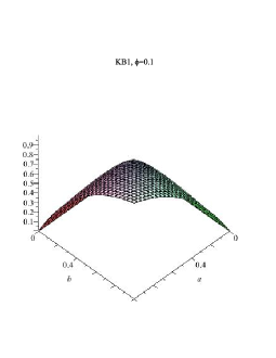
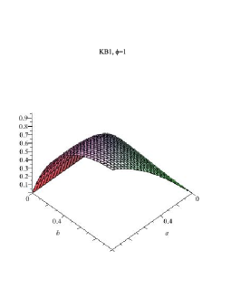
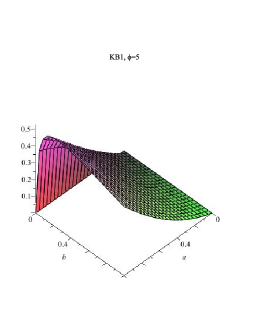
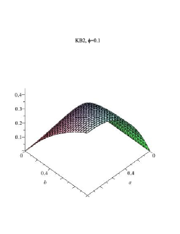
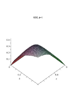
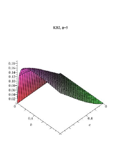
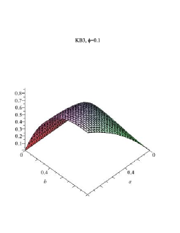
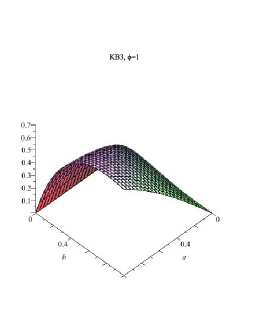
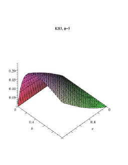
Figure 1: Kummer beta distributions for different $\phi$ parameter values

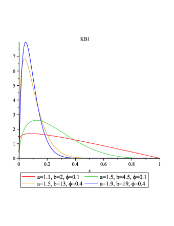
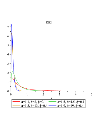
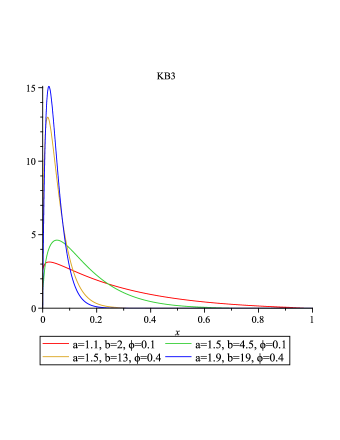
Figure 2: 2-dimensional representation for univariate Kummer beta distributions

4.2) According to Definition 1.1 all PK functions were functions of the trace argument, however it is also possible to extend the definition to include for example the PK function with the determinant as argument. In this regard, we propose the following definition.

Definition 4.4.

The random symmetric matrix $\bm{X}$ of dimension $m$ is said to have matrix variate beta generator distribution with parameters $a$, $b$ and $\bm{\Phi}$ and shape generator $h$, if it has the following density

1. (i) 1st kind

   $$f(\bm{X}) = \left(\sum_{t=0}^{\infty}\frac{h^{(t)}(0)B_{m}(a+t,b)}{t!}\det(\bm{\Phi})^{t}\right)^{-1}$$

   $$\det(\bm{X})^{a-\frac{1}{2}(m+1)}\det(\bm{I}_{m}-\bm{X})^{b-\frac{1}{2}(m+1)}\;h(\det(\bm{\Phi}\bm{X})),\quad\bm{X}\in\mathcal{I}_{m},$$

2. (ii) 2nd kind

   $$f(\bm{X}) = \left(\sum_{t=0}^{\infty}\frac{h^{(t)}(0)B_{m}(a+t,b-t)}{t!}\det(\bm{\Phi})^{t}\right)^{-1}$$

   $$\det(\bm{X})^{a-\frac{1}{2}(m+1)}\det(\bm{I}_{m}+\bm{X})^{-(a+b)}\;h(\det(\bm{\Phi}\bm{X})),\quad\bm{X}\in\mathcal{S}_{m},$$

3. (iii) 3rd kind

   $$f(\bm{X}) = \left(\sum_{t=0}^{\infty}\frac{h^{(t)}(0)B_{m}(a+t,b)}{2^{m(a+t)}t!}\det(\bm{\Phi})^{t}\right)^{-1}$$

   $$\det(\bm{X})^{a-\frac{1}{2}(m+1)}\det(\bm{I}_{m}-\bm{X})^{b-\frac{1}{2}(m+1)}\det(\bm{I}_{m}+\bm{X})^{-(a+b)}\;h(\det(\bm{\Phi}\bm{X})),\quad\bm{X}\in\mathcal{I}_{m},$$

   where $\mathop{\mathrm{R}e}\nolimits(a),\mathop{\mathrm{R}e}\nolimits(b)>(m-1)/2$, $\bm{\Phi}\in\mathcal{I}_{m}$ is a symmetric complex matrix, $h(.)$ is a Borel measurable function that admits a Taylor series expansion in zonal polynomials

4.3) It is known that the Wilks’ statistic plays the same role in multivariate analysis as the F statistic plays in univariate analysis. Bekker et al. (2011) derived an exact expression for the non-null distribution of the Wilks’ statistics. Bekker et al. (2012) proposed new multivariate test statistics and their exact distributions. Thus it is of interest to find the distribution of the determinant where the matrix variate has the MGB$i(i=1,2,3)$ distribution leading to generalized Wilks’ statistics.

Theorem 4.7.

Let $\bm{X}_{i}\sim MBGi_{m}(a,b,\bm{\Phi},h)$, $i=1,2,3$. Then

1. $y=\det(\bm{X}_{1})$ has the following density function

   $$f(y)=\zeta_{a,b}^{(1)}\Gamma_{m}(b)\sum_{t=0}^{\infty}\frac{h^{(t)}(0)}{t!}\sum_{\tau}C_{\tau}(\bm{\Phi})G_{m,m}^{m,0}\left(y\big{|}\begin{array}[]{c}c_{1},\ldots,c_{m}\\ d_{1},\ldots,d_{m}\end{array}\right),$$

   where $c_{j}=a+b+t_{j}-\frac{1}{2}(j+1)$ and $d_{j}=a+t_{j}-\frac{1}{2}(j+1)$.

2. $y=\det(\bm{X}_{2})$ has the following density function

   $$f(y)=\zeta_{a,b}^{(2)}\sum_{t=0}^{\infty}\frac{h^{(t)}(0)}{t!}\sum_{\tau}\Gamma_{m}(b,-\tau)C_{\tau}(\bm{\Phi})G_{m,m}^{m,0}\left(y\big{|}\begin{array}[]{c}c_{1},\ldots,c_{m}\\ d_{1},\ldots,d_{m}\end{array}\right),$$

   where $c_{j}=a+b+t_{j}-\frac{1}{2}(j+1)$ and $d_{j}=a+t_{j}-\frac{1}{2}(j+1)$.

3. $y=\det(\bm{X}_{3})$ has the following density function

   $$f(y)=\zeta_{a,b}^{(3)}\Gamma_{m}(b)\sum_{\tau,\kappa,\phi}\frac{(-1)^{k}h^{(t)}(0)\left(\theta_{\phi}^{\kappa,\tau}\right)^{2}}{t!k!C_{\tau}(\bm{I}_{m})}C_{\tau}(\bm{\Phi})G_{2m,2m}^{2m,0}\left(y\big{|}\begin{array}[]{c}c_{1},\ldots,c_{2m}\\ d_{1},\ldots,d_{2m}\end{array}\right),$$

   where

   $$c_{j} = \left\{\begin{array}[]{cc}a+b-1+\phi_{\frac{i+1}{2}}-\frac{1}{4}(i-1),&i=1,3,5,\ldots,2m-1\\ a+b-1-\frac{1}{4}(i-2),&i=2,6,10,\ldots,2m\end{array}\right.$$

   $$d_{j} = \left\{\begin{array}[]{cc}a+b-1+k_{\frac{i+1}{2}}-\frac{1}{4}(i-1),&i=1,3,5,\ldots,2m-1\\ a-1+\phi_{\frac{i}{2}}-\frac{1}{4}(i-2),&i=2,6,10,\ldots,2m\end{array}\right.$$

where $G(.)$ denotes the Meijer’s G function.

Proof: We only give the proof for item 1; the proofs of other two types are the same. Using Theorem 3.1, the Mellin transform is given by (see Mathai, 1993)

$$\mathcal{M}_{f}(r) \equiv E\left(\det(\bm{X})^{r-1}\right)$$

$$= \zeta_{a,b}^{(1)}\sum_{t=0}^{\infty}\frac{h^{(t)}(0)}{t!}\sum_{\tau}\frac{\Gamma_{m}(a+r-1,\tau)\Gamma_{m}(b)}{\Gamma_{m}(a+b+r-1,\tau)}C_{\tau}(\bm{\Phi}).$$

Thus the distribution of $y$ is uniquely obtained from the inverse Mellin transform of the above and the definition of the Meijer’s G-function, $G(.)$. The proof is complete. $\blacksquare$

In this paper we developed the conventional matrix variate beta distributions to more general ones, where the kernel of a matrix variate beta type 1/2/3 with a further Borel measurable function of scalar value were combined. Important statistical characteristics were derived such as the moment generating function as well as the joint density function of eigenvalues. The matrix variate Kummer beta distributions were discussed as special cases. The authors are currently developing more theory and results based on the principle of Definition 1.1 and the theory applied in the paper. The program of work will include amongst others the noncentral beta as kernel combined with numerous different generators (see Arashi et al., 2013 and Van Niekerk et al., 2013).

With the similar idea of generating new families of matrix-variate distributions, another families of distributions can be generated by utilizing the “Wishart-type kernels” combined with an unknown Borel measurable function of trace and/or determinant operators. In this case the algebra will need evaluating ”Laplace-type integrals” involving zonal polynomials. (Refer to Bekker et al., 2013)

We deem that the proposed results in this paper should stimulate research and applications beyond the known matrix variate distributions.

References

M. Arashi, A. Bekker, J. J. J. Roux, and J. Van Niekerk, (2013). Noncentral beta kernel oriented generator family. Technical Report, University of Pretoria, South Africa.

A. Bekker, J. J. J. Roux, and M. Arashi, (2011). Exact nonnull distribution of Wilks’ statistic: The ratio and product of independent components, J. Mult. Anal., 102, 619-628.

A. Bekker, J. J. J. Roux, R. Ehlers and M. Arashi, (2012). Distribution of the product of determinants of noncentral bimatrix beta variates, J. Mult. Anal., 109, 73-87.

A. Bekker, M. Arashi, J. J. J. Roux, and J. van Niekerk, (2013). Wishart kernel oriented generator distribution: Weighted Wishart distribution, Technical Report ISBN: 978-1- 77592-067-0, University of Pretoria, South Africa.

B. W. Brown, M. S. Floyd, L. B. Levy, (2002). The log F: a distribution for all seasons. Comput. Statist., 17, 47-58.

Yasuko Chikuse, (1980). Invariant polynomials with matrix arguments and their applications in Multivariate Statistical Analysis, 1, 54-68.

A. W. Davis, (1979). Invariant polynomials with two matrix arguments extending the zonal polynomials: Applications to multivariate distribution theory, Ann. Inst. Statist. Math., 31(A), 465-485.

A. W. Davis, (1980). Invariant polynomials with two matrix arguments, extending the zonal polynomials, Multivariate Ananlysis-V (ed. P. R. Krishnaiah), 287-299.

R. Ehlers, (2011). Bimatrix Variate Distributions of Wishart Ratios With Application, Unpublished PhD Dissertation, University of Pretoria.

M. Ferreia, M. I. Gomez, and V. Leiva, (2012). On an extreme value version of the Birnbaum-Sanders distribution, REVSTAT, 10(2), 181-210.

Arjun K. Gupta and Daya K. Nagar, (2000a). Matrix variate distributions, Chapman and Hall / CRC, Boca Raton.

Arjun K. Gupta and Daya K. Nagar, (2000b). Matrix-variate beta distribution, Int. J. Math. Sci., 24(7), 49-459.

Arjun K. Gupta and Daya K. Nagar, (2002). Matrix-variate Kummer-beta distribution, J. Aust. Math. Sci., 73, 11-25.

Arjun K. Gupta and Daya K. Nagar, (2006). A Generalized Matrix Variate Beta Distribution, Int. J. Appl. Math. Sci., 3(1), 21-36.

Arjun K. Gupta and Daya K. Nagar, (2009). Properties of matrix variate beta type 3 distribution, Int. J. Mathematics Math. Sci., http://dx.doi.org/10.1155/2009/308518.

A. T. James, (1961). Zonal polynomials of the real positive definite symmetric matrices, Ann. Math., 35, 456-469.

A. T. James, (1964). Distribution of matrix variate and latent roots derived from normal samples, Ann. Math. Statist., 35, 475-501.

M. C. Jones, (2004). Family of distributions arising from distribution of order statistics. Test 13, 1-43.

C. G. Khatri, (1966). On certain distribution problemsbased on positive definite quadratic functions in normal vector, Ann. Math. Statist., 37, 468-479.

P. Kvam, (2008). Length bias in the measurements of carbon nanotubes, Technometrics, 50(4), 462-467.

A. M. Mathai, (1993). A Handbook of Generalized Special Functions for Statistical and Physical Sciences, Clarendon Press, Oxford.

Rob J. Muirhead, (2005). Aspects of Multivariate Statistical Theory, 2nd Ed., John Wiley, New York.

S. Nadarajah and S. Kotz, (2004). The beta Gumbel distribution, Math. Prob. Eng., 10, 323-332.

S. Nadarajah and S. Kotz, (2006). The beta exponential distribution, Reliab. Eng. Syst. Saf., 91, 689-697.

S. Nadarajah and S. Kotz, (2006). Some beta distributions, Bull. Brazilian Math. Soc., New Series, 37(1), 103-125.

Daya K. Nagar and Arjun K. Gupta, (2002). Matrix-variate Kummer-beta distribution, J. Australian Math. Soc., 73(1), 11-25.

Daya K. Nagar, Alejandro Roldá-Correa and Arjun K. Gupta, (2013). Extended matrix variate gamma and beta functions, J. Mult. Anal., 122, 53-69.

A. K. Nanda and K. Jain (1999). Some weighted distribution results on univariate and bivariate cases, J. Statist. Plann. Inf., 77, 169-180.

J. Navarro, J. M. Ruiz and Y. DeL Aguila, (2006). Multivariate weighted distributions: a review and some extensions, Statistics, 40(1), 51-64.

K. W. Ng and S. Kotz, (1995). Kummer gamma and Kummer beta univariate and multivariate distributions, Research Report No. 84, (Department of Statistics, The University of Hong Kong, Hong Kong).

I. Olkin, and H. Rubin, (1962). A characterization of the Wishart distribution, Ann. Math. Statist., 33, 1272-1280.

J. Pauw, A. Bekker and J. J. J. Roux, (2010). Densities of composite Weibullized generalized gamma variables, S. Afr. Statist. J., 44, 17-42.

G. O. Silva, E. M. M. Ortega, and G. M. Cordeiro, (2010). The beta modified Weibull distribution, Lifetime Data Anal., 16, 409-430.

N. Singla, K. Jain, and S. K. Sharma, (2012). The beta generalized Weibull distribution: Properties and applications, Reliability Eng. Sys. Safety, 102, 5-15.

S. M. Sunoj, and M. N. Linu, (2012). Dynamic cumulative residual Renyi’s entropy, Statistics, 46(1), 41-56.

J. Van Niekerk, M. Arashi, A. Bekker and J. J. J. Roux, (2013). Wishart kernel oriented generator distributions with application, Technical Report, University of Pretoria, South Africa.

K. Zagrafos and S. Nadarajah, (2005). Expression for Rényi and Shannon entropies for multivariate distributions, Statist. Prob. Lett., 71, 71-84.