The general recombination equation
in continuous time and its solution
Ellen Baake
Technische Fakultät, Universität Bielefeld,
Postfach 100131, 33501 Bielefeld, Germany
, Michael Baake
Fakultät für Mathematik, Universität Bielefeld,
Postfach 100131, 33501 Bielefeld, Germany
and Majid Salamat
Technische Fakultät, Universität Bielefeld,
Postfach 100131, 33501 Bielefeld, Germany
Abstract.
The process of recombination in population genetics, in its
deterministic limit, leads to a nonlinear ODE in the Banach space of
finite measures on a locally compact product space. It has an
embedding into a larger family of nonlinear ODEs that permits a
systematic analysis with lattice-theoretic methods for general
partitions of finite sets. We discuss this type of system, reduce it
to an equivalent finite-dimensional nonlinear problem,
and establish a connection with an ancestral partitioning process,
backward in time. We solve the
finite-dimensional problem recursively for generic sets of parameters
and briefly
discuss the singular cases, and how to extend the solution to this
situation.
1. Introduction
This contribution is concerned with differential equation models for
the dynamics of the genetic composition of populations that evolve
under recombination. Here, recombination is the genetic mechanism in
which two parent individuals are involved in creating the mixed type
of their offspring during sexual reproduction. The essence of this
process is illustrated in Fig. 1 and may be
idealised and summarised as follows.
Genetic information is encoded in terms of finite sequences.
Eggs and sperm (i.e., female and male germ cells or
gametes) each carry one such sequence. They go through the
following life cycle: At fertilisation, two gametes meet randomly and
unite, thus starting the life of a new individual, which is equipped
with both the maternal and the paternal sequence. At maturity, this
individual generates its own germ cells. This process may include
recombination, that is, the maternal and paternal sequences perform
one or more crossovers and are cut and relinked accordingly, so
that two ‘mixed’ sequences emerge. These are the new gametes and start
the next round of fertilisation (by random mating within a large
population).
Figure 1. Life cycle of a
population under sexual reproduction and recombination. Each line
symbolises a sequence of sites that defines a gamete (such as the
two at the top that start the cycle as ‘egg’ and ‘sperm’). The
pool of gametes at the left and the right comes from a large
population of recombining individuals. These sequences meet
randomly to start the life of a new individual. Altogether, each
of these sequences has been pieced together from two randomly
chosen parental sequences.
Models of this process aim at describing the dynamics of the genetic
composition of a population that goes through this life cycle
repeatedly. These models come in various flavours: in discrete or
continuous time; with various assumptions about the crossover pattern;
and in a deterministic or a stochastic formulation, depending on
whether or not the population is assumed to be so large that
stochastic fluctuations may be neglected. We will employ the
deterministic continuous-time approach here, but allow for very
general crossover patterns.
The biologically relevant cases will be mentioned throughout the
paper, as will various connections to the existing body of literature.
From now on, we describe populations at the level of their gametes and
thus identify gametes with individuals. Their genetic information is
encoded in terms of a linear arrangement of sites, indexed by the set
. For each site , there is a set
of ‘letters’ that may possibly occur at that site. For the sake of
concreteness, we use finite sets for
the moment; we generalise this to arbitrary locally compact spaces
in Section 6.
A type is thus defined as a sequence , where is called the
type space. By construction, is the -th component
or coordinate of , and we define
as the collection of ‘coordinates’ with indices in , where is a
subset of . A population is identified with
(or described by) a probability
vector on , where denotes
the proportion of individuals of type in . Note that we assume
the sequences to have fixed length. Additional processes that may
change this, such as copying blocks, are disregarded here; see
[22] and references therein for possible extensions.
With Fig. 1 in mind, recombination may now be
modelled as follows. A new (‘offspring’) sequence is formed as the
‘mixture’ of two randomly chosen parental sequences (say and )
from the population: It copies the letters of at some of its sites
and those of at all others. If, for example, a double crossover
happens between sites and and between and (),
then the offspring sequence reads . The offspring
sequence replaces a randomly chosen sequence (possibly one of the
parents, but this is negligibly rare in a large population). Viewed
differently, the offspring sequence in our example reads whenever
the parents are of the form and . Here, a ‘’ at site stands for an arbitrary
element of , so means marginalisation. This will be helpful when
formulating the differential equation.
The sites that come from the paternal and the maternal sequences,
respectively, define a partition of into two
parts. Due to the random choice of the parents, we need not keep track
of which sequence was ‘maternal’ and which was ‘paternal’. In
principle, all partitions of into two parts ()
can be realised, via a suitable number of crossovers at suitable
positions. If no crossover happens, then the partition is , and the offspring is an exact copy of the first
parent. Reproduction with recombination according to a partition
happens at rate .
We shall introduce all notions with more care later. For now, we turn
the verbal description into a differential equation system and obtain
(1)
for all , where denotes the set of
partitions of into two parts. Eq. (1) may be
understood as a ‘mass balance’ equation: For every , sequences of type are ‘produced’ from the
corresponding parental sequences at overall rate , where the
product reflects the random combination; at the same time, sequences
of type are lost (i.e., replaced by new ones) at overall rate
. Note that the case provides no net contribution to , since gain
and loss are equal in this case.
The resulting ODE system appears difficult to handle, due to the large
number of possible states and the nonlinearity of the right-hand side.
In previous papers [6, 5, 4, 26, 3, 7, 8], we have
concentrated on a special case, namely, the situation in which at most
one crossover happens at any given time. That is, we restricted
attention to ordered partitions into two parts, corresponding
to the sites before and after a single-crossover point. We have
analysed the resulting models in continuous time (both deterministic
and stochastic), as well as in discrete time. For the deterministic
continuous-time system, a simple explicit solution is available
[6, 5]. This simplicity is due to some underlying linearity.
It is now time to tackle the case of general partitions (in continuous
time). Therefore, in this contribution, we give up the
single-crossover assumption – and even allow for an arbitrary number
of parents in a given recombination event, which leads to partitions
with more than two parts. Even though this is not a common biological
feature, we will see that it requires little extra mathematical
effort. Also, it is a very natural structure on the lattice of
partitions of a (finite) set.
The restriction to partitions form the biologically most relevant
subset will always be possible by a suitable choice
of the model parameters, which are the recombination rates
.
This contribution is motivated by the pioneering work of Geiringer
[18] and Bennett [10], who worked on a similar system in
discrete time (but restricted to a special type space);
the later work of Lyubich [19, Chapter 6], who worked out
much of the underlying structure and got close to
a solution in 1992; and by
more recent work of Dawson [12, 13], who presented a (recursive)
solution in
2000 and 2002. It relies on a certain nonlinear transformation from
(gamete or type) frequencies to suitable correlation functions, which
decouple from each other and decay geometrically. If sequences of more
than three sites are involved, this transformation must be constructed
via recursions that involve the parameters of the recombination
process.
Dawson’s construction testifies to remarkable insight into the
problem. However, it is not easy to penetrate to the mathematical core
of his arguments. We therefore start at the very beginning and
formulate the model on a fairly general type space, in a
measure-theoretic framework, and allowing for arbitrary partitions.
More importantly, we put the problem into a systematic
lattice-theoretic setting; this will become the key for the
transparent construction of the solution.
Furthermore, we establish a connection with a partitioning process
backward in time, which describes how an individual in the present
population has been pieced together from the genetic material of its
ancestors.
This provides a link to the ancestral recombination graph (ARG),
which is the ancestral process commonly used in models
of recombination in finite populations, see
[14, Ch. 3.4].
The paper is organised as follows. After introducing the mathematical
objects we need and some of their properties in
Section 2, the general recombination equation is
discussed in Section 3. As a first step, this is done
in the setting of a measure-valued ordinary differential equation
(ODE), which is then reduced to a finite-dimensional ODE
system. Section 4 solves this system under a linearity
assumption, which is motivated by previous work, but does not give
the solution in sufficient generality.
As a further preparation for the general solution, we study the
behaviour of the system under marginalisation in
Section 5.
Based on this, Section 6
establishes the connection with the partitioning
process. This is followed by the derivation
of the general solution in Section 7, which is
recursive in nature and applies to the generic choice of the
recombination rates. More detailed properties of the solution are
investigated in Section 8, while
Section 9 deals with various types of non-generic
cases. The Appendix provides some material for the treatment of
degenerate cases.
This paper builds on previous work, most importantly on
[6, 5]. Some of the results from these papers will freely be
used below, and not re-derived here (though we will always provide
precise references).
2. Partitions, measures and recombinators
Let be a finite set, and consider the lattice of
partitions of ; see [1] for general background on lattice
theory. When the cardinality of is , the set contains
elements, known as the Bell number; compare [23, A 000110]. With , these numbers are recursively computed
as for ,
with generating function and explicit formula . A subset of relevance to us,
for the biological applications, consists of all partitions of
into two parts, , which contains elements. Note
that generates the lattice in an obvious way.
Here, we write a partition of as , where is the number of its parts (or blocks), and one has for all together with . The natural ordering relation is denoted by
, where means that is
finer than , or that is coarser than .
The conditions and are
synonymous, while means together
with .
The joint refinement of two partitions and is written as
, and is the coarsest partition below and .
The unique minimal partition within the lattice is
denoted as , while the unique
maximal one is . When ,
we also employ the interval notation . For a general subset of
, we write the complement as . Finally, when , the coarsest partition below
all elements of is denoted by . Note that
by convention.
When and are disjoint (finite) sets, two partitions
and can be joined to form an
element of . We denote such a joining by
, and similarly for multiple joinings. Conversely, if
, a partition , with say, defines a unique partition of by
restriction. The latter is denoted by , and its parts
are precisely all non-empty sets of the form with
.
Let now and define , where each is a locally compact space. In many
concrete applications, the will be finite sets, but we do not
make such a restriction as it is neither necessary nor
desirable. In particular, there are situations in quantitative
genetics [11] that will profit from the more general setting
we employ here.
When and are given, we denote the natural projection to the
th component by , so . Similarly, for
an arbitrary non-empty subset , we use the notation
for the projection to the subspace .
Let denote the space of finite, regular Borel measures on
, equipped with the usual total variation norm , which
makes it into a Banach space. Also, we need the closed subset (or
cone) of positive measures, which we mean to include the
zero measure. Within , we denote the closed subset of
probability measures by . Note that and
are convex sets. The restriction of a measure to a subspace is written as , which is consistent with marginalisation of
measures. For any Borel set , one thus has the
relation .
Given a measure and a partition , we define the mapping by with and, for ,
(2)
where the product is (implicitly) ‘site ordered’, i.e. it matches the
ordering of the sites as specified by the set . We shall also use
site ordering for cylinder or product sets. We call a mapping of type
a recombinator. Note that recombinators are
nonlinear whenever .
Proposition 1.
Let and as above. Now, let be arbitrary, and consider the corresponding recombinator as
defined by Eq. (2). Then, the following assertions
are true.
(1)
is positive homogeneous of degree , which
means that holds
for all and .
(2)
is globally Lipschitz on , with
Lipschitz constant .
(3)
holds for
all .
(4)
maps into itself.
(5)
preserves the norm of positive measures,
and hence also maps into itself.
Proof.
Claims (1) and (4) are elementary consequences of the definition.
Claim (3) follows easily from the arguments used in
[6, Sec. 3.1], while (5) is clear from the observation that
for , which then implies by standard arguments; compare
[6, Fact 2].
It remains to prove (2). Let be a
partition with parts, where . Then,
one can show inductively in that
(3)
for arbitrary . If one of them is the zero
measure, the Lipschitz estimate is a consequence of claim (3).
Let now both be non-zero, and assume that
. Using Eq. (3)
together with positive homogeneity of , we have
(4)
where we used that and are measures of
norm . Next, one has
which, on inserting into Eq. (4), gives the inequality
from which our claim follows, with .
∎
Remark 1.
Let us mention that there is an alternative way to see the Lipschitz
property, at least for finite . This is because the dynamics may
then be reformulated in terms of a chemical reaction system. This is
a large class of models, for which a substantial body of theory is
available; see [24] for a review. In particular, the Lipschitz
property applies under very general conditions, which are satisfied
in our case.
The estimate used above is rather coarse, but suffices for our needs
here. When using the invariance of , one simply employs
Eq. (3) from the last proof to establish the
following consequence.
Corollary 1.
On , with , the
recombinator is
Lipschitz with . ∎
Before we embark on the recombination equation and its solution, we
need to establish one technical result on the relation between
recombinators and projectors to subsystems, as defined by non-empty
sets . Here, the system on which
a recombinator acts is marked by an upper index (for the full
system) or (for the subsystem). Later, we will drop this index
whenever the meaning is unambiguous.
Lemma 1.
Let be a finite set as above, and an arbitrary partition. If
is non-empty and , one has
where and the upper index of a
recombinator indicates on which measure space it acts.
Proof.
We shall show the claimed identity by verifying it for certain
‘rectangular’ measurable sets that suffice for the equality of the
two measures as Baire measures, and then rely on the unique
extension of Baire measures to regular Borel measures; compare the
discussion around [6, Fact 1]. To this end, let
be given as ,
and write as , where . Each is contained in
precisely one part of . Without loss of generality, we may
thus assume that for , while for all (when ,
this case does not occur).
Now, let be a Borel set in , and consider the corresponding ‘rectangular’
set , where we again assume that the product observes proper site
ordering. When evaluated on , the right-hand side of our claim
gives
where we have used that and where denotes a projector that is only
defined on the subspace . This is now to be compared
with the evaluation of the left hand side of the claim, which gives
(with )
which agrees with our previous expression and thus proves the claim.
∎
Lemma 1 has some interesting consequences for the
structure of recombinators. We only state the result and omit the
proof, as it is analogous to the corresponding result in [6].
Proposition 2.
Let . On , the corresponding
recombinators satisfy
In particular, each recombinator is an idempotent and any two
recombinators commute. ∎
Below, we shall also need probability vectors on , which
form the compact space . An interesting subclass of them can
be constructed as follows. Let
be a function on the lattice , and consider
(5)
for , which clearly satisfies .
Moreover, one has
(6)
wherefore , which means that is a probability
vector on the lattice .
At this point, we have gathered the core material to embark on the
discussion of the recombination equation and its properties.
3. The general recombination equation
With the tools at hand, it is now rather obvious how to generalise the
‘mass balance’ equation (1) of the Introduction to
our measure-theoretic setting. Within the Banach space , we thus consider the nonlinear ODE
(7)
with non-negative numbers that have the meaning of
recombination rates in our context. They are written in this
way because we consider
as an element of the Möbius algebra over ; see
[1, 25] for background. We will usually assume that an
initial condition for is given for
the ODE (7), and then speak of the corresponding
Cauchy problem (or initial value problem). Biologically,
Eq. (7) describes the change in composition of a
population in which offspring is produced by piecing together
sequences from various parents according to the collection of the
with . More precisely, with rate
for every , the sites in
inherited from parent are reassociated with the sites in
inherited from parent , and with the sites in inherited
from parent for .
Remark 2.
Since , the value of is
immaterial, and the corresponding term could clearly be omitted on
the right-hand side of Eq. (7). We nevertheless keep
it here, as it will become useful in connection with the reduction
to subsystems.
Another way to write the ODE is
with being the total
recombination rate.
With , we can now simply write
(8)
but we must keep in mind that is a nonlinear operator.
Nevertheless, one has the following basic result; compare [2]
for background on ODEs on Banach spaces.
Proposition 3.
Let be a finite set and the corresponding locally
compact product space as introduced above. Then, the Cauchy problem
of Eq. (7) with initial condition has a unique solution. Moreover, the cone is forward invariant, and the flow is norm-preserving on
. In particular, is forward invariant under
the flow.
Proof.
By part (2) of Proposition 1, all are globally Lipschitz on , which is then also true
of . Therefore, the uniqueness statement for the Cauchy
problem is clear.
Next, let and consider an arbitrary Borel set
with . Then, with as above in
Remark 2, we have
because by assumption and all other terms are non-negative
as a result of part (4) of Proposition 1 together
with for all . Positive
invariance of the closed cone now follows from a classic
continuity argument; see [2, Thm. 16.5 and Rem. 16.6] for
details and [6, Thm. 1] for the analogous argument in the
single-crossover model.
When is a positive measure, one has as a consequence of Proposition 1, and hence
which implies the preservation of the norm of a positive measure under
the forward flow. The last claim is then obvious.
∎
In view of our underlying biological problem, we restrict our
attention to the investigation of the recombination equation on the
cone , and on in particular. To proceed, we
will first bring the ODE (7) into a simpler form. To
this end, observe the structure of , which suggests that, as
the flow proceeds forward in time from an initial measure , the solution picks up fractions of components of the form
for various or even all ,
depending on which recombination rates are positive and which
partitions can thus be reached in the course of time.
Let and fix some . Now, define the
(finite-dimensional) set
which is the closed convex set that consists of all convex linear
combinations of the measures with . In fact, when the rates run through all
non-negative values, is the smallest closed
convex set that contains all measures which can be reached in the
course of recombination from the initial measure . The dimension
of depends on the nature of , and can even
be . When the dimension is maximal (meaning , which is
the generic case), is a simplex and the
measures are the extremal measures of the
simplex in the sense of convex analysis. Observe that
holds for any , which follows from a straightforward
though slightly technical calculation (details of which are given
below). This now suggests the ansatz
(9)
for the solution of our above Cauchy problem, with (generic) initial
condition and coefficient functions ,
the latter thus with .
For each , we view as an element of the Möbius algebra. We shall prove a
posteriori that the strategy of Eq. (9) works, and
that the original Banach space ODE is thus reduced to a
finite-dimensional system of ODEs, whose solution consists of a
one-parameter family of probability vectors on . The case of
non-generic initial conditions will be discussed afterwards.
To proceed, we now have to calculate the action of on a
general measure . It is convenient to
first consider probability measures, as the extension to general
positive measures is then immediate via the positive homogeneity of
the recombinators. So, let , which means
. Consider a single partition and observe that
where we have used Lemma 1 in the last step.
Observing that the product measure in the last expression is a measure
of the form for some with
, and that each such must occur here, we
see that
(10)
where we use a dot under a symbol to mark it as the summation
variable, thus following the notation of [1]. Next, if
, Proposition 1 implies that
are two equivalent ways to write .
Consequently, we extend our previous formula as
(11)
where we define the function as
(12)
for any with , and as
otherwise. In Eq. (12),
may be any real vector of dimension , even though we have only
considered positive ones above. Also, one has for consistency.
Remark 3.
When is a probability vector on , one has . The right-hand side of
Eq. (11) can then be read as a product of
marginalised probabilities for the subsystems defined by the
parts of the partition . This structure will be made
explicit in Section 5 (see
Lemma 1 in particular) and will later pave the way
to a recursive solution of the recombination equation.
For fixed , the function is an element of
the incidence algebra of our lattice over the field
. Following [1], we denote this algebra by , with convolution as multiplication. The latter is defined
as
Note that this definition automatically gives if , as it must. Important
elements of include the unit , defined
by , the zeta
function , defined by for
and otherwise, and the
Möbius function , which is the multiplicative (left
and right) inverse of . One then has . We refer to [25] for details and more
advanced aspects of incidence algebras.
With and , Eq. (11) allows us
to continue as follows,
(13)
which is the desired action of on elements of .
Inserting Eq. (9) into the recombination equation
(7) now gives the following result.
Lemma 2.
The ansatz (9) for the solution
of the recombination equation (7)
on leads to a system of induced ODEs for the
coefficient functions , namely
Clearly, Eq. (14) is the result of a
comparison of coefficients, based on the original equation
(7), its short form (8), and
Eq. (13). For a generic , this is
justified by the fact that the measures
with then are the extremal measures of the
forward-invariant simplex . Since the set of
generic is dense in , and the solution of the
Cauchy problem depends continuously on the initial condition, the
extension to all is consistent.
∎
Note that our above calculation was based upon the action of
recombinators on positive measures, because we have used
Lemma 1. Consequently, we do not know how
Eqs. (7) and (14) are related
beyond this case. Fortunately, this is not required, as the next
result shows, where we use .
Proposition 4.
The ODE system defined by Eq. (14), with
as in Eq. (12), is of dimension
, and has a unique solution for its Cauchy problem.
The closed cone is
invariant in forward time, and the -norm of
non-negative initial conditions is preserved. In particular, the
simplex of probability vectors on is
invariant in forward time.
Proof.
The ODE system of Eq. (14) can be written
as , where is
nonlinear. The first claim is clear, while solution uniqueness
once again follows from Lipschitz continuity of , which is
obvious here.
Let
be arbitrary and consider any subset
such that . Then, one has
since by assumption and all as
well as all are non-negative. This gives the
invariance of under the forward flow by standard
arguments [2, Thm. 16.5].
Repeating the calculation for yields
Now, the last sum (for any fixed ) is
(15)
as follows from Eq. (11) by taking norms on both
sides and observing that for all as well as , while one has for
any ; alternatively, one can also verify this
with a direct calculation on the basis of the definition of .
Consequently, , which implies
the claimed norm preservation. The positive invariance of
is then clear.
∎
Remark 4.
Observing that holds for any
, one can rewrite the ODE of
Eq. (7) as
which corresponds to the observation made in Remark 2.
With Proposition 4, we may now conclude that
our ansatz (14) is consistent and suitable
for the reduction of the original problem to a finite-dimensional one.
Theorem 1.
The one-parameter family of measures is a solution of the Cauchy problem of
Eq. (7) with initial condition if and only if it is of the form
where the coefficient functions satisfy the Cauchy problem of
Eq. (14) with initial condition
.
Proof.
The solution property is clear from our above calculations, while
the correspondence of the initial conditions is obvious for the
generic case, and extends to the general case by a standard
continuity argument. The claim now follows from the uniqueness
statements for the two Cauchy problems.
∎
Remark 5.
Let us mention that an alternative path to
Theorem 1 is possible via [2, Thm. 16.5 and
Rem. 16.6], by showing that the convex set
is forward invariant for any as initial
condition. This requires the verification of the ‘inside reflection
property’ for any piece of the boundary of ,
which is somewhat tedious in view of the possible degeneracies. This
is the reason why we opted for our approach above.
Let us briefly discuss the structure of for a
general , including the non-generic cases. Each
gives rise to a set of partitions
which is non-empty (since for all ) and
defines a unique partition
so that . The partition also defines the sublattice of
product form, with elements. It is precisely this
sublattice of that determines the structure of the convex
set , which is now the Cartesian product of
simplices, and of total dimension .
It is clear that the time evolution of a measure
under the flow of the recombination equation (7) can
thus be reduced to a smaller ODE system, which is fully consistent
with our above treatment as a consequence of
Eq. (10), as then means that effectively
only partitions from the set are involved. We leave it to
the reader to spell out the details for the modified correspondence
and the appropriate initial conditions for the finite-dimensional ODE
system.
We are now in the position to approach a solution of the recombination
equation.
4. Solution under a linearity
assumption
The relatively simple solution structure in the case of
single-crossover dynamics (see references [6, 5]) was due to the
fact that the nonlinear recombinators acted linearly along
solutions. Since this is a special case of our general model, via
setting for any that fails to be an ordered
partition with (at most) two parts, it is reasonable to consider this
point of view also more generally. It will turn out that the linearity
assumption is false in general, but we can still learn some
interesting things along the way.
Thus, let us assume that also the more general
recombinators act linearly along the solution. A simple calculation
shows that our coefficient functions then have to satisfy the ODEs
(16)
for all , where, for any fixed ,
(17)
is another element of the incidence algebra . The
difference of Eq. (16) to the general equation
(14) thus lies in the replacement of the
function by the significantly simpler linear function
.
Proposition 5.
The Cauchy problem defined by Eq. (16) together with
the initial condition has the unique solution given by
which, for , constitutes a one-parameter family of
probability vectors on .
Proof.
Consider the (upper) summatory function , which is
and hence satisfies the simple ODE
(18)
together with the initial condition for all .
On the other hand, for fixed with
, we have
wherefore the summatory function of the right-hand side of
Eq. (16), evaluated at , becomes
which agrees with the right-hand side of Eq. (18).
The claim now follows from (upper) Möbius inversion, because, for
all and for all , one has
(19)
where denotes the Möbius function for the
lattice .
The fact that , for each , is a probability
vector on follows from our earlier calculation in
Eq. (5), with .
∎
This approach clearly has a lattice-theoretic basis, which lends
itself to a number of interesting further aspects and insights
[9].
Remark 6.
Let us note that Eqs. (18) and
(19) allow a re-interpretation of the coefficient
formula from Proposition 5 as
(20)
with
being the decay rate of the corresponding (exponential)
term. This relation means , so that the recombination rates are
obtained from the decay rates by means of (upper) Möbius inversion
as
where it is assumed that the total recombination rate is
known. This detail corresponds to the fact that
does not contribute to any of the .
Either version of permits the determination of the asymptotic
properties of the coefficients as , and hence that
of the measure . In particular, when the partition
subset satisfies
, one has
with convergence in the -topology. This is the obvious
generalisation of the known asymptotic properties in the special
cases treated in [11, 6].
Remark 7.
Let us briefly mention that the linear system of ODEs defined by
Eq. (16) can still be solved when the recombination
rates become time-dependent, as was previously observed in
[5, Addendum] for single-crossover recombination. Indeed, if
all are non-negative functions of time
(which is needed to preserve all claims of
Proposition 4 also for
Eq. (16) with time-dependent rates), the solution
formula from Proposition 5 becomes
for the same initial conditions. The proof is completely analogous to
that of Proposition 5, now with
Let be or a partition into
two parts, one of which is a singleton set. Then, the coefficient
formula from Proposition 5 gives the correct
solution also for the Cauchy problem of the general recombination
equation from Eq. (14).
Proof.
Let a probability vector on be given. The definitions
of and from Eqs. (15) and
(17) imply, via a simple calculation, that
holds for any . This gives the claim for , because Eqs. (14) and
(16) are equal in this case, hence
.
More generally, when for some , one finds that
so that the ODEs from Eqs. (14) and
(16) coincide also for such partitions , which
proves the second claim.
∎
Corollary 2.
The coefficient formula from Proposition 5
gives the correct solution of Eq. (14) for
all whenever is a finite set
with .
Proof.
There is nothing to prove for . The claim for is
obvious, and also follows from [5, Prop. 3]. When , all
partitions except satisfy the conditions of
Theorem 2. Since , the claim follows.
∎
Remark 8.
In the special situation of single-crossover recombination, where
only for ordered partitions into
two parts, the solution formula of Proposition 5
reduces to the known solution for this case from [6, 5]. In
particular, the linearity assumption is satisfied, and the solution
holds for all system sizes and all values of the single-crossover
rates.
Note, however, that already for , when we are beyond the
single-crossover case, the coefficients and can
differ, for instance for , which is a
biologically relevant partition. We thus need to proceed without the
linearisation assumption.
5. General case: Marginalisation consistency
It is clear that our general recombination equation can only be
considered a reasonable model if it is marginalisation
consistent. By this we mean that the restriction to a subsystem,
via appropriate marginalisation, gives a solution of the recombination
equation for the subsystem. We now discuss this in more detail, and
then establish this consistency property for our model, both in the
measure-theoretic and in the finite-dimensional version. The latter
case will depend on an interesting interplay between elements of the
Möbius and the incidence algebras at hand.
Let be as above, or any other finite set with elements, and
consider a subsystem as specified by . When is the solution of the general recombination
equation (7) with initial condition according to Proposition 3, it is natural
to define
(21)
as the corresponding (marginalised) measure for the subsystem defined
by . Then, recalling that the projector is linear,
we get
where the fourth step is an application of Lemma 1,
while the last step anticipates the definition of the induced
(or marginal )
recombination rates for the subsystem as
(22)
for any . It is obvious that non-negativity of the
rates implies that of the marginal rates .
Our little calculation proves the following result.
Proposition 6.
Let be a finite set and a non-empty subset.
If is a solution of the recombination equation
(7), with recombination rates for and with initial condition
, the marginalised measure
from Eq. (21) solves the
recombination equation for the subsystem defined by ,
provided the recombination rates for
are defined according to
Eq. (22). ∎
Remark 9.
The problem of marginalisation consistency has been observed early
on in mathematical population genetics. Ewens and Thomson [16]
have tackled it in 1977 in models that describe the combined action
of recombination and selection for the two-parent case in
discrete time; see also the review in
[11, pp. 69–72]. The corresponding dynamics is, in
general, not marginalisation consistent. However, it is
obvious from the calculations in [16] that consistency does
apply in the case without selection, and the dynamics is then
governed by the marginal recombination probabilities, which are the
two-parent, discrete-time analogues of our marginal recombination
rates.
Let us see how this result translates to the finite-dimensional ODE
systems at the level of the coefficient functions .
Given a general probability vector on , we define
the corresponding marginal probabilities via
(23)
for any partition , in complete analogy to
Eq. (22).
Clearly, one has , while proper normalisation follows from
(24)
where the penultimate step follows from the observation that the inner
sum over consists of precisely one term because the restriction
of a partition to a subset is unique.
Let us note for later use that, for and , we also have
(25)
because
As special cases of Eqs. (23) and
(25), let us also note that, for
and , one has
(26)
Remark 10.
The (upper) summatory function defined by can also be calculated
by marginalisation, namely as
wherefore consistency at this level is obvious.
Let us return to the recombination rates for
together with
compare Remark 2, and consider the marginal rates
with and . Repeating the above calculation of the normalisation
condition, one finds
(27)
as it should be. The total recombination rate is thus the same on all
levels, and independent of , as it must. Note that, in this
process, need
not vanish. This does not matter because the corresponding
recombinator (on the subsystem) is the identity, and hence does not
affect the solution; compare Remark 2.
Let us now see how the result of
Proposition 6 translates to properties of
the coefficients for the ODE system and its subsystems. Here, the
desired marginalisation consistency will depend on the following
slightly technical, but somewhat surprising identity.
Lemma 3.
Let be as before, and let
with be arbitrary, but fixed. Then, for
any with , one has the
product representation and reduction relation
where is any probability vector on ,
its marginalisation according to Eq. (23), and
is defined as in Eq. (12), but with
replaced by .
Proof.
Let with be given, and
assume . With our definition of
the -function in Eq. (12) together with
Eqs. (26) and (23),
the right-hand side evaluates as
(28)
For an arbitrary with and , this is now to be compared
with
(29)
where the last step is once again a consequence of
Eq. (23). To proceed, we now rewrite the partition
as with and
for (which is
without loss of generality) and for . Note that is
possible, in which case no is present and .
Now, any partition in the summation in
Eq. (29) must be a joining of the form
with and
, subject to
the additional condition that we always have ,
which means for
all . The summation on the right-hand side of
Eq. (29) can now be broken into smaller sums that
can be absorbed into the factors, which amounts to refining each block
of individually. This turns the right-hand side of
Eq. (29) into a product of two terms, namely
Now, the sum in each factor of the second product is clearly
because is a probability vector on
, compare Eq. (24).
Consequently, the entire second term is , which is also true if
(in which case we have the empty product here). Likewise, the
sum in the th factor of the first product equals by Eq. (26),
because by our assumptions. We thus get
Together with Eqs. (28) and (29),
this proves the lemma.
∎
The marginalisation consistency can now be stated as follows.
Proposition 7.
Let be a finite set and a non-empty
subset. If the family of probability vectors is a solution of the Cauchy problem of
Eq. (14) with initial condition
, the marginalised
family , with
defined according to
Eq. (23) for all , solves the
corresponding Cauchy problem for the subsystem, with initial
condition and the
marginal recombination rates of
Eq. (22). Explicitly, it satisfies the ODE
(30)
The analogous statement remains true for a general probability
vector as initial condition, with the marginalised
initial condition according to
Eq. (23) on the subsystem.
Proof.
Let be a solution of
Eq. (14), and let be
fixed. Then, we have
where we have used Lemma 3 in the second-last step.
This made the -term independent of , which in turn
allowed the last step on the basis of Eq. (22)
and another application of Lemma 3. The second-last
step shows that the marginalised family indeed satisfies the proper
ODE for the subsystem as defined for
via Eq. (14), as it must; the last step then
leads to Eq. (30).
It is an easy exercise that is the
initial condition for the subsystem that emerges as the
marginalisation of the original initial condition . Since was arbitrary, the main
statement is proved. The last claim is an obvious generalisation.
∎
Note that Proposition 7 can also be viewed as
a consequence of Proposition 6 and
Theorem 1. We have nevertheless opted for an
explicit verification because several steps of the above proof will
reappear when we proceed to a solution of the recombination equation.
6. The backward point of view: Partitioning process
Now that we have understood the structure of the ODE for in
the usual (forward) direction of time, let us consider a related
(stochastic) process that will provide an additional meaning for
. Let be a Markov
chain in continuous time with values in that is constructed
as follows. Start with . If the current state is
, then part of is replaced by at rate , independently of all
other parts. That is, the transition from to occurs at rate for for
all and . Obviously, is a
process of progressive refinements, which we call the
partitioning process. Likewise, we define the partitioning
process on for
in the same way as
, but based on the marginal
recombination rates .
Now let , where denotes
probability. That is, is the transition
probability (in standard notation) from ‘state’ to ‘state’
during a time interval of length . Since
is a process of progressive
refinements, it is obvious that
(31)
Furthermore, since the parts are (conditionally) independent
once they appear, we have
(32)
Let us now consider the distribution of , that
is, the collection . Clearly, the initial value is . The time evolution is given by
(33)
Here, the first step is an application of the Kolmogorov
backward equation (for background, see [17, Ch. XVII.8] or
[21, Ch. 2.1]), namely, the decomposition according to the
first transition away from , which is to state with rate
for all . The second step uses
Eqs. (31) and (32). The
argument is illustrated in Figure 2.
Figure 2. A sketch of the partitioning process. Each
dot represents one part of the corresponding partition, while the
lines indicate the partitioning.
Comparing Eq. (33) with Eq. (30), we see that
the quantities and , with and , satisfy the same
collection of ODEs, and the initial values also agree at . By an obvious inductive argument, the two families
can thus be identified. We have therefore shown the following result.
Theorem 3.
The probability vector agrees with the distribution
of the partitioning process . Explicitly, we
have
for all , and all
. ∎
As the reader may have noticed, the partitioning process was defined
so as to reflect the action of recombination on the ancestry of the
genetic material of an individual backward in time. Namely, if
a sequence is pieced together according to a partition from various parents forwards in time, this implies
that the sequence is partitioned into the parts of when we look
backwards in time, where each part is associated with a different
parent. In this light, Theorem 3 means the following:
If we follow the ancestry of the genetic material of an individual
from the present population (that is, starting at time ) backward
in time, then is the probability that the sites are
partitioned into different parents according to at time
before the present. That is, the sites in go back to one
individual in the initial population, the sites in go back to a
second individual and so on, and the sites in go back to an
th individual. The partitioning process is the deterministic limit
of the corresponding stochastic process in finite populations, namely,
the ancestral recombination graph (ARG); see
[14, Ch. 3.4], but note that the ARG is usually described
for single crossovers only.
At the same time, the above suggests a nice interpretation of the
solution of the recombination equation in
Theorem 1. Indeed, the type distribution at
present may be obtained in a two-step procedure. In the first step,
one decides how the sites of a present individual have been pieced
together from different parents from the initial population. In the
second step, one assigns letters to the various parts (that is,
parents): If the corresponding partition is , then the letters for the sites in are drawn from
, and so on, until the letters
for the sites in are drawn from — and this independently, due to the infinite
population. The resulting type distribution of our individual today
is . What we have described here in words
amounts to a duality relation between the recombination
dynamics forward in time and the partitioning process backward in
time. We do not go into detail here; for more, see [8] and
[15].
7. Generic case: Recursive solution
Motivated by the Möbius formula in Eq. (20) and by a
reminiscent structure in the solution of the discrete recombination
equation, compare [3], we now restrict
Eq. (14) to the forward-invariant simplex
, compare Proposition 4, and
make the ansatz
(34)
for any non-empty , with decay rates and coefficient functions . Our aim is to
determine by a comparison of coefficients once we
know a (recursive) formula for the rate function
together with linear independence of the exponentials in
Eq. (34). Note that this will then also solve the ODE
(14) with an initial condition from via multiplying the right-hand side of
Eq. (34) by the norm of the initial condition.
From our results of Section 4, see
Theorem 2 and
Remark 6 in comparison
with Eq. (34), we know that
(35)
Note that we have used the fact that for all ,
which is obvious.
In particular, this gives for any with
, which is the trivial limiting case with an empty sum on the
right-hand side. All other values are now defined recursively by
(36)
which is motivated by the well-known eigenvalues in the two-parent,
discrete-time analogue of our model; see [19, Theorem 6.4.3] or
[20]. In the context of our partitioning process, is the total rate of any further partitioning of part ,
and so, due to the independence of the parts,
is the total rate of transitions out of state . For any with
, one has ,
while one finds for all non-empty
. This is consistent with the fact that no further
partitioning (or ‘decay’) is possible when starting from the partition
of .
The decay rates defined this way have important summation properties
as follows.
Lemma 4.
Let be a finite set and
be arbitrary, but fixed. If is a
partition of , with , one has . If is the number of the parts of
that are singletons, this can be simplified as
In particular, holds for all non-empty
.
Moreover, for arbitrary with
, one has
Proof.
The first claim follows from the relation , where does
not depend on as a consequence of
Eq. (27). For any part that is a singleton, one
has , which implies the
second identity. The latter, in turn, confirms that for all , since in
this case.
For the remaining identity, fix . If is a
refinement of , we have and must be a
joining of the form
with for all . Writing , we have because
implies the existence of a bijection between the
two families and
. Eq. (36) now implies
that the right-hand side of our claim is
holds for any . For larger , this relation holds
for and any with if one of the
parts is a singleton set, as follows from
Theorem 2.
Lemma 5.
Let the decay rates with
be distinct and assume that the recombination rates for subsystems
are calculated according to Eq. (22). Then,
for any non-empty , the decay rates with are distinct as well. In this case,
the exponential functions with
are linearly independent over .
Proof.
Assume distinctness of the rates with and fix a non-empty . If exist with but , we may choose with , (hence ) and
. Since , we can employ Lemma 4 to
derive that
which is a contradiction to the distinctness assumption. This proves
the first claim, while the second assertion is standard.
∎
Below, we need to understand the decay rates in various ways. Let us
thus expand on their relation with the recombination rates. Starting
from the definition in Eq. (36), with , one
obtains
(38)
where denotes the characteristic function
of the condition in its subscript.
Lemma 6.
The decay rates defined in Eq. (36) are linear
functions of the recombination rates of the form
, with
In particular, the coefficients are
non-negative integers, and one has
if and only if .
Proof.
The first claim summarises our calculation in
Eq. (38). It is obvious from the explicit formula
that , for all . The coefficient vanishes if and only if each condition
under the summation is true, which means for all . But
the latter condition, in turn, is equivalent with , which proves the assertion.
∎
Remark 11.
One important consequence of Lemma 6 is
that, as linear functions of the recombination rates, and are different whenever ,
because the intervals and are then
different, too. By a standard Baire category argument, the
situation that the rates with are
distinct is then generic. In fact, the exceptional set with any
degeneracy among the decay rates is a union of true hyperplanes in
parameter space . Consequently, it is both a
nowhere dense set and a null set. The corresponding statement
remains true if we restrict our attention to the parameter space .
Let us now return to the original ansatz (34). The
coefficient function is an element of the incidence
algebra . Since is our initial condition, we see that, for and any , we must have
hence (as mentioned above)
together with
(39)
for . This way, for non-empty and
, the coefficients are
either fixed or recursively determined from with .
which has to be compared with the right-hand side of
Eq. (30). Inserting the corresponding expression for the
coefficients of the subsystem according to our ansatz yields the
expression
where the second part of Lemma 4 was used
in the last step. Inserting the expression (34)
for , changing
summation variables and regrouping terms gives
(41)
where the second step effectively removes all terms with
; compare Remark 2.
Let be non-empty and let us assume that the
exponential functions on the right-hand side of
Eq. (34) are linearly independent. By
Lemma 5, this is certainly the case when the rates
with are distinct; compare
Remark 11. Now, a comparison of coefficients in
Eq. (41) with those of the right-hand side of
Eq. (40) yields the relations
for all with . Note that our
assumption entails the condition that for all , so that we
get
(42)
for all , where the
-coefficients for the subsystems are themselves determined
recursively, under the distinctness condition for the subsystem decay
rates, which follows from our assumption by
Lemma 5. Since we know for any
with from Corollary 2 and
Remark 6, see also
Corollary 5 below, the recursion
(42) uniquely determines all -coefficients.
We have thus shown the following result for the generic situation
of Remark 11.
Theorem 4.
Let be a finite set, and assume that the decay
rates with are distinct. Let
the decay rates for non-empty subsets be
defined via Eqs. (35) and (36),
where the marginal recombination rates on subsystems are given by
Eq. (22).
Then, our exponential ansatz (34) solves the Cauchy
problem of Eq. (14) with initial
condition if and only
if the coefficients are recursively determined
by Eq. (42) together with and Eq. (39). ∎
Let us mention in passing that a similar result can be derived for
other initial conditions as well. We concentrate on this one as it
fits Theorem 1 and thus also provides a solution
of the original recombination equation.
Remark 12.
The recursion in Eq. (42), and the solution thus
constructed for the recombination dynamics, is similar in structure
to the corresponding relations (6.5.1) and (6.5.2) in Lyubich’s book
[19] for the two-parent case in discrete time. However, in
contrast to our ’s, Lyubich’s coefficients depend on
. As noted in [19], this dependence on the
initial condition poses a serious difficulty to the solution, since
it makes an explicit iteration impossible. Put differently, our
approach achieves the complete separation of the recombination
structure from the types, as already inherent in
Theorem 4 and further discussed in
Section 6; this entails a crucial
simplification.
In the situation of Theorem 4, we thus know that our
original ansatz (34) leads to a solution. Since we
then also know that holds only for ,
and otherwise, we have the following
immediate consequence for the asymptotic behaviour of the solution.
which means that the corresponding solution of
the ODE (7), with initial condition
, -converges to the equilibrium
as . Moreover, the
convergence is exponentially fast, with the rate given by , while the individual rate
for the convergence of is given by . ∎
The recursive nature of our solution does not immediately help
to understand its structure and meaning. Let us thus study some
aspects of it in more detail.
8. Generic solution: Structure and further properties
To begin, let us observe that Theorem 4 has an
interesting consequence which contrasts the result of
Lemma 6 and shows a surprising structural
similarity with the corresponding relation of
Remark 6.
Corollary 4.
Let be as in Theorem 4 and assume that the
decay rates with are distinct.
Then, the recombination and the decay rates are related by
and the corresponding relation holds for any subsystem
that is defined by a non-empty .
Proof.
By Theorem 4 and
Proposition 4, we know that the ansatz of
Eq. (34), for , leads to the unique solution
of the ODE (14) with initial condition
. Thus, we may equate the
right-hand side of Eq. (14) with that of
Eq. (40), again for , and consider the
resulting identity at . Observing that
holds for our probability vector as a result of
Eq. (12), the first claim is clear.
The second assertion follows by the corresponding calculation with
, which is justified by
Proposition 7 together with
Lemma 5.
∎
Note that the relation of Corollary 4 is a
nonlinear one, because the -coefficients themselves generally
depend on the recombination rates. To make any further progress, we
need to better understand these coefficients, beyond and the relations in Eq. (39).
Proposition 8.
Under the assumptions of Theorem 4, one finds the
following properties.
(1)
for all non-empty
;
(2)
holds for all ;
(3)
Assume further that is strictly positive on all
partitions of with two parts. Then, for all and all non-empty
; In particular, is then an
invertible element of the incidence algebra for
over .
Proof.
For the first claim, observe that for any with
, so in this case. Assume now that the claim is true for all with
, and consider a larger set, say. With , we then get from Eq. (42) that
where the second step uses the induction hypothesis (note that we
always have ), while the last step
employs Eq. (37) which applies here.
Next, the normalisation property of the implies
Since and since the decay rates with are distinct by our assumption together
with Lemma 5, the functions are linearly independent. Consequently, the last
identity is equivalent to the second claim.
For the third claim, recall that the dimension of the ODE system
(14) is if the set of partitions
with generates the entire
lattice , which is the case under our assumptions. The convex
set that is spanned by the solution functions is then a
simplex of dimension , and the normalisation condition
is the only linear relation
between these functions.
We already know that , and one easily
finds
for any with . One may now
proceed inductively in the number of parts. If there were some
with , where we may assume
to be the coarsest partition with this property, we would get
from Eq. (34) an additional linear relations among
the solution functions , which is impossible. Since
by the second assertion, the claim is
true on the top level (defined by ). Repeating the argument
for any non-empty completes the argument.
Finally, the invertibility of as an element of the
incidence algebra is a standard consequence of
claim (3); compare [1].
∎
Consequently, under the assumptions of part (3) of
Proposition 8, has a unique (left
and right) inverse, say. This means that
holds for all . The coefficients are
thus determined by
together with the recursion
for , which derives from the left equality above.
Alternatively, one may use the corresponding formula that derives from
the other identity.
Either from direct calculations, or by invoking the results from
Section 4, in particular
Theorem 2 and Corollary 2,
the following result is obvious (see the text after
Remark 3 for the definitions of and ).
Corollary 5.
For any with , one has
, and hence also . For larger sets , one has for and for all with
two parts, if one of them is a singleton set. In the latter case,
also .
Proof.
Corollary 2 implies the first claim, while
Theorem 2 gives the second one for
as well as for any with two parts, provided one of
them is a singleton set. The last claim follows from .
∎
Let us now define
(43)
which is an analogue of the summatory function from
Section 4 (see the proof of
Proposition 5). Using , we now obtain
(44)
hence for all as a consequence of ; compare
Lemma 4. One difference to the linear case is that
the summation weights in Eq. (43) generally depend
on the recombination rates, while they were constant (in fact, given
by the -function of the incidence algebra) in
Section 4. Due to the properties of the decay rates
, one inherits the corresponding relations among the
coefficient functions for . In particular,
together with
determines all coefficients, while Lemma 4
implies the additional relation
for any with .
Note that the function generally does not emerge
from via marginalisation in the sense of
Eq. (22), which is another important
difference to the special situation of Section 4 and
Remark 10.
Lemma 7.
Let denote the coefficients from
Theorem 4 in the case of distinct rates, and
assume that for all
with two parts, so that is an invertible element of
the incidence algebra. Then, for any non-empty , one has the following properties.
(1)
;
(2)
holds for all
;
(3)
holds for all and all .
Proof.
The invertibility of is clear from part (3) of
Proposition 8, while is a consequence of the first assertion
of the same proposition.
Next, we already know that . For , we can proceed inductively via the standard inversion
formula [1] for , which gives
where the second step employs the induction hypothesis while the
second assertion of Proposition 8 was used in the
penultimate step.
The third claim is a consequence of the initial conditions together
with Eqs. (43) and (44), because
holds for any .
∎
It is quite clear that the structure of is somewhat simpler
than that of . At present, we have defined as the
inverse function to in the incidence algebra, but it would be
nice to also have a direct way to calculate it, for instance via
another recursion.
9. Some comments on the singular cases
Our focus in the previous section was on the generic case that
allowed for a recursively defined, general solution. Let us now
briefly look into what happens when certain degeneracies among
the decay rates occur.
Recall that our ansatz (34) requires, a priori, the
linear independence of the exponential functions , and thus the distinctness of the decay rates
, for , separately for all non-empty
. A posteriori, we need to understand what happens
when two decay rates, as functions of the recombination rates
of the system on the top level, become equal. Once
again, this is best looked at inductively. If satisfies , we are in the
realm of the ‘linear’ solution of Section 4, and no
consequences emerge from degeneracies. In other words, the solution
formula from Proposition 5 is valid for all
values of the recombination rates, irrespective of possible
degeneracies; compare Corollaries 5 and
2.
When we step up in system size, there can be degeneracies that are
still ‘harmless’ in the sense that the -coefficients extend
continuously to these situations. In this case, the (now reduced) set
of exponentials in Eq. (34) is still sufficient, and
the solution valid. However, as is evident from
Eq. (42), the situation changes when for some , as we then hit a
singularity. To understand the underlying phenomenon, let us assume
that corresponds to the smallest subsystem where this type of
‘bad’ degeneracy occurs. Now, rewrite Eq. (41) as
with . Note that the are well-defined
for all and all values of the recombination
rates, because only -coefficients of subsystems smaller than
occur in the product. We are now in the standard situation of
ODE theory that we have summarised in Lemma 8 of the
Appendix: Precisely when for
some , we need an additional function for our ansatz,
namely . So, our original
ansatz (34) no longer suffices, and has to be
modified accordingly. At the same time, in line with our previous
observation, additional degeneracies of the form with are harmless.
Now, this dichotomic structure continues on each new level: There are
‘harmless’ degeneracies that do not require additional functions for
our ansatz, while degeneracies of the type once again render the function set of the ansatz
incomplete, even one that was augmented in the previous
step. Lemma 9 of the Appendix reviews a typical case,
while the remarks following it show how the degenerate case produces
extra monomial factors of increasing exponents for each degeneracy of
the ‘bad’ type. At this point, we hope that the general structure is
sufficiently clear, so that we can leave further details to the
reader.
Let us summarise our discussion as follows.
Corollary 6.
If is a finite set as before, the generic recursive solution
from Theorem 4 extends to all recombination
rates , with , such that
holds for all non-empty
and all . ∎
Appendix
Here, we state some useful results from classical ODE theory, whose
proofs are straightforward exercises that are left to the reader.
Lemma 8.
Let and
be non-negative real numbers. Then, the Cauchy problem defined by
the ODE
together with the initial condition has the
unique solution
where
is a smooth function that is non-negative for all and
symmetric under the exchange of the two parameters and
. ∎
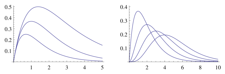
An illustration of the function is shown in the left
panel of Figure 3. A similar type of result emerges for
mixtures of exponentials with higher order monomials.
Figure 3. Left panel: Illustration of the function
of Lemma 8 for
and three values of , namely (top curve),
(middle) and (bottom). Right panel: Illustration of for parameters
(from left to right).
Lemma 9.
Let and be non-negative real numbers, and . Then, the Cauchy problem
with initial condition has the unique solution
, where
is a smooth non-negative function for all . ∎
Some examples are illustrated in the right panel of
Figure 3. By standard results from ODE theory, it is
clear how to combine the results of Lemmas 8 and
9 to cover further situations. Let us only add that the
ODE
with initial condition has the unique solution
which explains the appearance of monomial factors with increasing
powers in the solution of such equations with degenerate rates.
Acknowledgements
MB would like to thank Roland Speicher for valuable discussions. We
thank an anonymous reviewer for his insightful and constructive
comments. This work was supported by the German Research Foundation
(DFG), within the SPP 1590.
References
[1]
M. Aigner,
Combinatorial Theory, reprint,
Springer, Berlin (1997).
[2]
H. Amann,
Gewöhnliche Differentialgleichungen,
2nd ed., de Gryuter, Berlin (1995).
[3]
E. Baake,
Deterministic and stochastic aspects of single-crossover recombination,
in: Proceedings of the International Congress of Mathematicians,
Hyderabad, India, 2010, Vol. VI, ed. J. Bhatia,
Hindustan Book Agency, New Delhi (2010), pp. 3037–3053;
arXiv:1101.2081.
[4]
E. Baake and I. Herms,
Single-crossover dynamics: Finite versus
infinite populations,
Bull. Math. Biol.70 (2008) 603–624;
arXiv:q-bio/0612024.
[5]
M. Baake,
Recombination semigroups on measure spaces,
Monatsh. Math.146 (2005) 267–278
and 150 (2007) 83–84 (Addendum);
arXiv:math.CA/0506099.
[6]
M. Baake and E. Baake,
An exactly solved model for mutation, recombination
and selection,
Can. J. Math.55 (2003) 3–41
and 60 (2008) 264–265 (Erratum);
arXiv:math.CA/0210422.
[7]
E. Baake and T. Hustedt,
Moment closure in a Moran model with recombination,
Markov Proc. Rel. Fields17 (2011)
429–446;
arXiv:1105.0793.
[8]
E. Baake and U. von Wangenheim,
Single-crossover recombination and ancestral recombination trees,
J. Math. Biol.68 (2014) 1371-1402;
arXiv:1206.0950.
[9]
M. Baake and R. Speicher, in preparation.
[10]
J.H. Bennett,
On the theory of random mating,
Ann. Human Gen.18 (1954) 311–317.
[11]
R. Bürger,
The Mathematical Theory of Selection, Recombination
and Mutation, Wiley, Chichester (2000).
[12]
K.J. Dawson,
The decay of linkage disequilibrium under random union of
gametes: How to calculate Bennett’s principal components,
Theor. Popul. Biol.58 (2000) 1–20.
[13]
K.J. Dawson,
The evolution of a population under recombination: How to linearise the dynamics,
Lin. Alg. Appl.348 (2002) 115–137.
[14]
R. Durrett,
Probability Models for DNA Sequence Evolution,
2nd ed., Springer, New York (2008).
[15]
M. Esser, S. Probst and E. Baake,
Partitioning, duality, and linkage disequilibria in the Moran
model with recombination,
submitted; preprint arXiv:1502.05194.
[16]
W.J. Ewens and G. Thomson,
Properties of equilibria in multi-locus genetic systems,
Genetics87 (1977) 807–819.
[17]
W. Feller,
An Introduction to Probability Theory and Its Applications,
Vol. I, 3rd ed., Wiley, New York (1986).
[18]
H. Geiringer,
On the probability theory of linkage in Mendelian heredity,
Ann. Math. Stat.15 (1944) 25–57.
[19]
Y.I. Lyubich,
Mathematical Structures in Population Genetics,
Springer, Berlin (1992).
[20]
T. Nagylaki, J. Hofbauer and P. Brunovski,
Convergence of multilocus systems under weak epistasis or
weak selection,
J. Math. Biol.38 (1999) 103–133.
[22]
O. Redner and M. Baake,
Unequal crossover dynamics in discrete and
continuous time,
J. Math. Biol.49 (2004) 201–226;
arXiv:math.DS/0402351.
[23]
N.J.A. Sloane,
The On-Line Encyclopedia of Integer Sequences,
OEIS Foundation; online available via
https://oeis.org/
[24]
E. D. Sontag,
Structure and stability of certain chemical networks and applications
to the kinetic proofreading model of T-cell receptor signal
transduction,
IEEE Trans. Automatic Control46 (2001), 1028–1047;
arXiv:math.DS/0002113.
[25]
E. Spiegel and C.J. O’Donnell,
Incidence Algebras,
Marcel Dekker, New York (1997).
[26]
U. von Wangenheim, E. Baake and M. Baake,
Single-crossover recombination in discrete time,
J. Math. Biol.60 (2010) 727–760;
arXiv:0906.1678.