Elliptic Waves in Two Component Long Wave–Short Wave Resonance Interaction System in One and Two dimensions

Abstract

We consider (2+1) and (1+1) dimensional long-wave short-wave resonance interaction systems. We construct an extensive set of exact periodic solutions of these systems in terms of Lamé polynomials of order one and two. The periodic solutions are classified into three categories as similar, mixed, superposed elliptic solutions. We also discuss the hyperbolic solutions as limiting cases.

1 Introduction

The study of nonlinear waves is of broad scientific interest [1]. Nonlinear waves in multi component long-wave-short-wave resonant interaction (LSRI) system have received significant attention in recent years. Here nonlinear resonance interaction between a low frequency long-wave (LW) and multiple high frequency short-waves (SWs) takes place when the phase velocity (say $v_{p}$) of the former exactly or approximately matches with the group velocity (say $v_{g}$) of the short-waves, that is, $v_{p}$ $\simeq$ $v_{g}$. This LSRI phenomenon has a wide range of applications ranging from water waves to nonlinear optics which also include bio-physics and plasma physics. In the SW components the soliton is formed due to a delicate balance between the dispersion and the nonlinear interaction of LW with the SWs while in the LW component, the soliton formation is determined solely by the self-interaction of short wave-packets.

The pioneering work of LSRI system was done by Zakharov [2]. Later on, the general Zakharov equations in one dimension have been reduced to the integrable Yajima-Oikawa system in Ref. [3]. At the same time, independently Benney has derived the model equation for the interaction of short wind-driven capillary gravity wave in deep water [4]. The experimental study of LSRI in a three layer fluid was carried out by Kopp and Redekopp [5]. Then, in a physical set up of two layer fluid model the one and two dimensional LSRI systems have been derived and bright and dark soliton solutions have also been obtained in Refs. [6, 7].

Recently, Kanna et al. have shown that the following (1+1) dimensional (i.e. one time and one space dimensions) LSRI system [8]

$$iS_{j,t}+\delta S_{j,xx}+LS_{j}=0,\quad\quad j=1,2,$$ (1a)

$$L_{t}=2\displaystyle\sum_{j=1}^{2}c_{j}|S_{j}|^{2}_{x},$$ (1b)

can be deduced from a set of three coupled nonlinear Schrödinger equations governing the propagation of three optical fields in a triple mode optical fiber, by applying the asymptotic reduction procedure. In eq. (1), $S_{j}$ and $L$, respectively, indicate $j^{th}$ short wave and (one) long wave, $t$ and $x$ represent the partial derivatives with respect to evolutional and spatial coordinates, respectively, and the nonlinearity coefficients $c_{j},j=1,2,$ are arbitrary real parameters. Here $\delta=\pm 1$ and for $\delta=1$ the above system (1) is nothing but the two component Yajima-Oikawa (YO) system. Eq. (1) also appears in the study of interaction of quasi resonant two frequency short wave pulses with a long wave [9]. Such multi-component YO system also has been derived in the context of multiple component magnon-phonon system [10]. In Ref. [8], we have obtained the bright n-soliton solution of the above system (1) and have revealed the fact that the bright solitons can undergo two types of fascinating energy sharing collisions. Here the presence of the long wave induces nonlinear interaction between two SWs which leads to nontrivial collision behaviour. The rogue waves of LSRI system with $j=1$ (one SW and LW components) and $\delta=1$ have been reported in Ref. [11].
The two dimensional multi-component LSRI system has also received equally good attention as that of their one-dimensional counterpart. Particularly the following two component analogue of the (2+1) dimensional (i.e. two spatial coordinates $x$, $y$ and one time coordinate) LSRI system

$$i[S_{j,t}+\varepsilon_{j}S_{j,y}]+\delta~{}S_{j,xx}+LS_{j}=0,\quad j=1,2,$$ (2a)

$$L_{t}=2\displaystyle\sum_{j=1}^{2}c_{j}|S_{j}|^{2}_{x},$$ (2b)

where the subscripts $x$ and $y$ represent the partial derivatives with respect to spatial coordinates and $t$ represents temporal coordinate, the nonlinearity coefficients $c_{1}$ and $c_{2}$ and the co-efficient $\varepsilon_{j}$, $j=1,2$, are real arbitrary parameters and $\delta=\pm 1$. Eq. (2) has been derived as the governing equation for the interaction of three nonlinear dispersive waves in optical fiber or in photorefractive medium by applying a reductive perturbation method [12]. In the above system, two SWs propagate in anomalous dispersion regime and the real long wave propagates in the normal dispersion regime. In a recent work [13], Kanna et al. have generalized the approach of [12] and derived a $M$-component LSRI system as the propagation equation for multiple dispersive waves (say $(M+1)$ waves ) in a weak Kerr type nonlinear medium in the small amplitude limit. To get further physical insight into the above system (2), we would like to point out that the one component ($j=1$) version of Eq. (2) can be derived from the governing equation for two-dimensional two wave interaction [14, 15] by following the approach of [12]. Thus system (2) is a three- wave generalization of two wave system in (2+1) dimensions. From a mathematical perspective, the soliton solutions of system (2), with $c_{1}=c_{2}=1$ are constructed in Refs. [12, 16]. Particularly, in Ref. [16] it has been shown that the bright solitons exhibit interesting energy sharing collisions characterized by intensity (energy) redistribution, amplitude dependent phase-shifts and change in relative separation distances.

Periodic nonlinear waves can also arise in real physical systems. For example, generation of ultrashort pulse-train by using nonlinear transform of a twin frequency signal is one such real system arising in nonlinear optics ([17] and references there in). Thus to describe real situations one may need special type of periodic solutions. Several periodic solutions of integrable and nonintegrable mullticomponent nonlinear Schrödinger equations with focusing, defocusing and mixed type nonlinear interactions have been obtained in Refs. [17]-[26], in terms of Jacobi elliptic functions. So far, such elliptic wave solutions have not been constructed for the one- and two- dimensional two component LSRI systems (1) and (2) as these integrable systems have been reported recently. This paper is aimed at constructing different families of elliptic wave solutions of (1) and (2) in a systematic way.

The organization of the paper is as follows. In section 2, the elliptic wave solutions of the $(2+1)$ dimensional two component LSRI system (2) are obtained in terms of Lamé polynomials of orders one and two. Similar solutions of $(1+1)$ dimensional two component LSRI system (1) are dicussed in section 3. Finally, conclusions are drawn in the last section.

2 Jacobi Elliptic function solutions of the (2+1)-dimensional two component LSRI system

We start with the $(2+1)$ dimensional LSRI system (2). To construct the Jacobi elliptic solutions of eq. (2a) we choose the travelling wave ansatz

$$S_{j}(x,y,t)=f_{j}[\beta(x-vt-wy+\delta_{0})]e^{-i(\omega_{j}t+\nu_{j}y-k_{j}x+\delta_{j})}, j=1,2.$$ (3)

Here $f_{j}$ are real functions of $x$, $y$ and $t$; $\beta,\delta_{0}$ and $\delta_{1,2}$ are real constants, $\omega_{j}$ is the frequency of the $j^{th}$ SW component, $k_{j}$ is the wave number, $v$ is the velocity, $w$ and $\nu_{j}$ are real parameters. Note that both the short waves are travelling with the same velocity. Inserting the above ansatz (3) into Eq. (2b), we obtain the LW component as

$$L=-\frac{2}{v}(c_{1}|S_{1}|^{2}+c_{2}|S_{2}|^{2}).$$ (4)

Following this, by substituting the ansatz (3) into (2) and also by using (4), we get a set of complex equations. On equating the real and imaginary parts, we respectively obtain

$$\frac{d^{2}f_{j}}{du^{2}}+\left[\frac{\delta(\omega_{j}+\varepsilon_{j}\nu_{j})-k_{j}^{2}}{\beta^{2}}-\frac{2\delta}{v\beta^{2}}\left(c_{1}f_{1}^{2}+c_{2}f_{2}^{2}\right)\right]f_{j}=0,\;\;\;j=1,2,$$ (5a)

$$v+\varepsilon_{j}w=2\delta k_{j},\qquad\qquad\qquad\qquad\qquad\qquad$$ (5b)

where $u=\beta(x-vt-wy+\delta_{0})$. At a first look it might seem that (5) is similar to the coupled nonlinear Schrödinger system given in [19]. But a careful analysis shows that they are essentially different. This is due to the presence of the long wave component $L$. In fact, here the solution parameters $\beta$ and the velocity $v$ explicitly appear before the non-linear term $(c_{1}f_{1}^{2}+c_{2}f_{2}^{2})$ . This makes the present system different from that of [19]. Particularly, this $v$ determines the nature of the solution, i.e., whether the solution is singular or not, as will be shown later. Thus the results presented here are distinct from those given in [19], though the elliptic function solutions take standard Lamé function profiles as will be demonstrated below. These solutions can be viewed as velocity locked solutions.
Next, we assume the Lamé function ansatz for $f_{j}$, that is,

$$f_{j}=\rho_{j}\psi_{j}^{(l)},\quad\quad l,j=1,2,$$ (6)

where $\psi_{j}^{(l)}$ can be anyone of the three first order Lamé polynomials for $l=1$ and for $l=2$, it can be any one of the five second order Lamé polynomials and satisfy the Lamé equation [27],

$$\frac{d^{2}\psi_{j}^{(l)}}{du^{2}}+[\lambda_{j}^{(l)}-l(l+1)m{\rm sn}^{2}(u,m)]\psi_{j}^{(l)}=0,$$ (7)

where $m$ ($0\leq m\leq 1$) is the modulus parameter of the Jacobi elliptic function ${\rm sn}(u,m)$,  $l~{}(=1,2)$ represents the order of the Lamé polynomial $\psi_{j}^{(l)}$ and $\lambda_{j}^{(l)}$ is the corresponding eigenvalue. Thus we will have two distinct families of solutions corresponding to the Lamé polynomials of order 1 ($l=1$) and of order 2 ($l=2$). First, we present and discuss periodic solutions in terms of Lamé polynomials of order one and then we present the second order solutions.

2.1 Solutions in terms of Lamé polynomals of order 1

The two component LSRI system (2) admits seven distinct periodic solutions in terms of Lamé polynomials of order 1. These first order solutions of Eq. (2) corresponding to $l=1$ can be expressed in terms of Jacobi elliptic functions [28]. We classify these solutions as similar, mixed and superposed elliptic solutions. By similar we mean same kind of standard elliptic function profile for both the short wave components. For the mixed elliptic solutions, the two short wave components take distinct elliptic function profiles. The superposed solutions are special and they are constructed by superposition of two elliptic functions. Apart from these elliptic functions, we also discuss the hyperbolic (soliton/solitary wave) solutions by fixing the modulus parameter $m$ as one.

2.1.1 Similar elliptic solutions

The similar elliptic solutions are listed in Table 1.

Table 1: Similar elliptic solutions of order 1

Similar	$f_{1}(u)$	$f_{2}(u)$	Constraints on	Long wave
elliptic	$S_{1}=f_{1}$	$S_{2}=f_{2}$	parameters	component
solutions	$\times e^{-i(\omega_{1}t+\nu_{1}y-k_{1}x+\delta_{1})}$	$\times e^{-i(\omega_{2}t+\nu_{2}y-k_{2}x+\delta_{2})}$
(1)	$A~{}\textit{{\rm dn}(u,m)}$	$B~{}\textit{{\rm dn}(u,m)}$	$v+\varepsilon_{1}w=2\delta k_{1},~{}v+\varepsilon_{2}w=2\delta k_{2}$,	$\left(2\delta\beta^{2}\right){\rm dn}^{2}(u,m)$
			$\beta^{2}=-\delta\frac{\left(c_{1}A^{2}+c_{2}B^{2}\right)}{v}>0$,
			$\omega_{1}+\varepsilon_{1}\nu_{1}-\delta\left(k_{1}^{2}-(2-m)\beta^{2}\right)=0$,
			$\omega_{2}+\varepsilon_{2}\nu_{2}-\delta\left(k_{2}^{2}-(2-m)\beta^{2}\right)=0$.
(2)	$A~{}\sqrt{m}~{}\textit{{\rm cn}(u,m)}$	$B~{}\sqrt{m}~{}\textit{{\rm cn}(u,m)}$	$v+\varepsilon_{1}w=2\delta k_{1},~{}v+\varepsilon_{2}w=2\delta k_{2}$,	$\left(2\delta m\beta^{2}\right){\rm cn}^{2}(u,m)$
			$\beta^{2}=-\delta\frac{\left(c_{1}A^{2}+c_{2}B^{2}\right)}{v}>0$,
			$\omega_{1}+\varepsilon_{1}\nu_{1}-\delta\left(k_{1}^{2}-(2m-1)\beta^{2}\right)=0$,
			$\omega_{2}+\varepsilon_{2}\nu_{2}-\delta\left(k_{2}^{2}-(2m-1)\beta^{2}\right)=0$.
(3)	$A~{}\sqrt{m}~{}\textit{{\rm sn}(u,m)}$	$B~{}\sqrt{m}~{}\textit{{\rm sn}(u,m)}$	$v+\varepsilon_{1}w=2\delta k_{1},~{}v+\varepsilon_{2}w=2\delta k_{2}$,	$\left(-2\delta m\beta^{2}\right){\rm sn}^{2}(u,m)$
			$\beta^{2}=\delta\frac{\left(c_{1}A^{2}+c_{2}B^{2}\right)}{v}>0$,
			$\omega_{1}+\varepsilon_{1}\nu_{1}-\delta\left(k_{1}^{2}+(1+m)\beta^{2}\right)=0$,
			$\omega_{2}+\varepsilon_{2}\nu_{2}-\delta\left(k_{2}^{2}+(1+m)\beta^{2}\right)=0$.

In Table 1, $(u,m)=(\beta(x-vt-wy+\delta_{0}),m)$. The long wave solutions are also given in the last column of Table 1. Each of the above solutions contains fifteen real parameters along with five constraints. Note that the period of second and third solution is twice that of first solution. The amplitudes of solution (1) for the two SW components are A and B while that of solutions (2) and (3) are $A\sqrt{m}$ and $B\sqrt{m}$. The distinction of the present solutions from the solutions of coupled nonlinear Schrödinger equations [19] mainly lies in the constraint conditions which significantly alters the nature of the solutions. Particularly, to get regular solution, we require $\beta^{2}$ to be positive. Once the signs of $c_{1}$ and $c_{2}$ as well as $\delta$ are fixed this can be achieved by suitably choosing the sign of $v$. To get insight into another physical aspect of the present solutions, let us consider the constraint expression for $\beta^{2}$ in solution (1) with $c_{1}=c_{2}=1$, for simplicity. Then one can find $A^{2}+B^{2}=-\frac{\beta^{2}v}{\delta}$, $\delta=\pm 1$. This indicates that for a given value of $\frac{\beta^{2}v}{\delta}$ any change in intensity (square of the amplitude) in one SW component will in turn influence the intensity of the other. Thus the solution displays intensity exchange. Ultimately, intensity of a particular SW component can be enhanced by suppressing that of the other component. Same conclusion can be drawn for the solutions (2) and (3) too. Such kind of intensity sharing depending upon the velocity is a special feature of the present two-component LSRI system.

2.1.2 Mixed elliptic solutions

The mixed elliptic solutions admitting different profiles of elliptic wave trains in the the short wave components $S_{1}$ and $S_{2}$ of Eq. (2) are tabulated below.

Table 2: Mixed elliptic solutions of order 1

Mixed	$f_{1}(u)$	$f_{2}(u)$	Constraints on	Long wave
elliptic	$S_{1}=f_{1}$	$S_{2}=f_{2}$	parameters	component
solutions	$\times e^{-i(\omega_{1}t+\nu_{1}y-k_{1}x+\delta_{1})}$	$\times e^{-i(\omega_{2}t+\nu_{2}y-k_{2}x+\delta_{2})}$
(1)	$A~{}\textit{{\rm dn}(u,m)}$	$B~{}\sqrt{m}~{}\textit{{\rm sn}(u,m)}$	$v+\varepsilon_{1}w=2\delta k_{1}$,	$-2~{}[\left(\frac{c_{2}}{v}\right)~{}B^{2}$
			$v+\varepsilon_{2}w=2\delta k_{2}$
			$\beta^{2}=\delta\frac{\left(c_{2}B^{2}-c_{1}A^{2}\right)}{v}>0$,	$-\delta\beta^{2}{\rm dn}^{2}(u,m)]$
			$\omega_{1}+\varepsilon_{1}\nu_{1}-\delta\left(k_{1}^{2}+m\beta^{2}\right)-\frac{2}{v}c_{1}A^{2}=0$,
			$\omega_{2}+\varepsilon_{2}\nu_{2}-$
			$\delta\left(k_{2}^{2}+(1+m)\beta^{2}\right)-\frac{2}{v}c_{1}A^{2}=0$.

(2)	$A~{}\sqrt{m}~{}\textit{{\rm cn}(u,m)}$	$B~{}\sqrt{m}~{}\textit{{\rm sn}(u,m)}$	$v+\varepsilon_{1}w=2\delta k_{1}$,	$-2[\left(\frac{c_{2}}{v}\right)~{}m~{}B^{2}$
			$v+\varepsilon_{2}w=2\delta k_{2}$,	$-m\delta\beta^{2}{\rm cn}^{2}(u,m)]$
			$~{}~{}\beta^{2}=\delta\frac{\left(c_{2}B^{2}-c_{1}A^{2}\right)}{v}>0$,
			$\omega_{1}+\varepsilon_{1}\nu_{1}$
			$-\delta\left(k_{1}^{2}+\beta^{2}\right)-\frac{2}{v}mc_{1}A^{2}=0$,
			$\omega_{2}+\varepsilon_{2}\nu_{2}$
			$-\delta\left(k_{2}^{2}+(1+m)\beta^{2}\right)-\frac{2}{v}mc_{1}A^{2}=0$.
(3)	$A~{}\textit{{\rm dn}(u,m)}$	$B~{}\sqrt{m}~{}\textit{{\rm cn}(u,m)}$	$v+\varepsilon_{1}w=2\delta k_{1}$,
			$v+\varepsilon_{2}w=2\delta k_{2}$,	$2~{}[\left(\frac{(1-m)}{v}\right)~{}c_{2}~{}B^{2}$
			$\beta^{2}=-\delta\frac{\left(c_{1}A^{2}+c_{2}B^{2}\right)}{v}>0$,	$-\delta\beta^{2}{\rm dn}^{2}(u,m)]$
			$\omega_{1}+\varepsilon_{1}\nu_{1}$
			$-\delta\left(k_{1}^{2}-m\beta^{2}\right)+\frac{2}{v}(1-m)c_{1}A^{2}=0$,
			$\omega_{2}+\varepsilon_{2}\nu_{2}$
			$-\delta\left(k_{2}^{2}-(1-2m)\beta^{2}\right)+\frac{2}{v}(1-m)c_{1}A^{2}=0$.

In the above table, $(u,m)=(\beta(x-vt-wy+\delta_{0}),m)$. Here the solutions are characterized by fifteen real parameters along with five constraints. As in the similar solutions the intensity sharing property is exhibited by the above solutions. This is evident from the expression for $\beta^{2}$ in the column ”constraint on parameter” in Table 2.

2.1.3 Superposed elliptic solution

The two component LSRI system (2) admits the following superposed elliptic solution [29]:

$$S_{1}(x,t) = \left[\frac{1}{2}(A~{}\textit{{\rm dn}(u,m)}+D~{}\sqrt{m}\textit{{\rm cn}(u,m)})\right]e^{-i(\omega_{1}t+\nu_{1}y-k_{1}x+\delta_{1})},$$ (8a)

$$S_{2}(x,t) = \left[\frac{1}{2}(B~{}\textit{{\rm dn}(u,m)}+E~{}\sqrt{m}\textit{{\rm cn}(u,m)})\right]e^{-i(\omega_{2}t+\nu_{2}y-k_{2}x+\delta_{2})},$$ (8b)

$$L = \left(\frac{\delta\beta^{2}}{2}\right)(\textit{{\rm dn}(u,m)}~{}\pm~{}\sqrt{m}~{}\textit{{\rm cn}(u,m)})^{2}.$$ (8c)

Here the parametric restriction can be expressed as

$$v+\varepsilon_{1}w=2\delta k_{1},~{}v+\varepsilon_{2}w=2\delta k_{2},~{}D=\pm A,~{}E=\pm B,~{}\beta^{2}=-\delta\frac{\left(c_{1}A^{2}+c_{2}B^{2}\right)}{v}>0,$$

$$~{}\omega_{1}+\varepsilon_{1}\nu_{1}-\delta\left(k_{1}^{2}-\frac{(1+m)}{2}\beta^{2}\right)=0,~{}~{}\omega_{2}+\varepsilon_{2}\nu_{2}-\delta\left(k_{2}^{2}-\frac{(1+m)}{2}\beta^{2}\right)=0.$$ (8d)

Here the signs of $D$ and $E$ are correlated i.e. for $D=A~{}(D=-A)$, $E=B~{}(E=-B)$.

2.1.4 Hyperbolic solution($m=1$)

(a) In the limit $m=1$, mixed elliptic solutions (1) and (2) of Table 2 go over to the hyperbolic solution

$$S_{1} = \left[A~{}{\rm sech}(\beta(x-vt-wy+\delta_{0}))\right]~{}e^{-i(\omega_{1}t+\nu_{1}y-k_{1}x+\delta_{1})},$$ (9a)

$$S_{2} = \left[B~{}\tanh(\beta(x-vt-wy+\delta_{0}))\right]~{}e^{-i(\omega_{2}t+\nu_{1}y-k_{2}x+\delta_{2})},$$ (9b)

$$L = -2\left[\frac{c_{1}A^{2}}{v}+\delta\beta^{2}\tanh^{2}(\beta(x-vt-wy+\delta_{0}))\right],$$ (9c)

with the parametric restriction

$$v+\varepsilon_{1}w=2\delta k_{1},~{}v+\varepsilon_{2}w=2\delta k_{2},~{}\beta^{2}=\delta\frac{\left(c_{2}B^{2}-c_{1}A^{2}\right)}{v}>0,$$

$$\omega_{1}+\varepsilon_{1}\nu_{1}-\delta\left(k_{1}^{2}+\beta^{2}\right)-\frac{2}{v}c_{1}A^{2}=0,~{}\omega_{2}+\varepsilon_{2}\nu_{2}-\delta\left(k_{2}^{2}+2\beta^{2}\right)-\frac{2}{v}c_{1}A^{2}=0.$$ (9d)

Here the SW components $S_{1}$ and $S_{2}$ are comprised of bright and dark solitary waves, respectively while the LW component is comprised of anti-dark (bright solitary wave with non-zero asymptotics) solitary wave. In Eq. (2), the nonlinearity is said to be of focusing type, if the co-efficients ($c_{1},c_{2}$) of nonlinearity and $\delta$ appearing before the dispersion term admit same sign. In that case, usually the system (2) admits bright soliton solution. But here the nonlinear interaction of SWs with LW leads to the possibility of such mixed (bright-dark) solitary wave solution in system (2) even with focusing type nonlinearities.
(b) Further, the mixed elliptic solution (3) of Table 2, the similar elliptic solutions (1) and (2) given in Table 1 and superposed elliptic solution (8) reduce to the hyperbolic (localized solitary wave/soliton) form given below:

$$S_{1} = \left[A~{}{\rm sech}(\beta(x-vt-wy+\delta_{0}))\right]~{}e^{-i(\omega_{1}t+\nu_{1}y-k_{1}x+\delta_{1})},$$ (10a)

$$S_{2} = \left[B~{}{\rm sech}(\beta(x-vt-wy+\delta_{0}))\right]~{}e^{-i(\omega_{2}t+\nu_{2}y-k_{2}x+\delta_{2})},$$ (10b)

$$L = \left(2\delta\beta^{2}\right){\rm sech}^{2}(\beta(x-vt-wy+\delta_{0})),$$ (10c)

along with parametric restriction

$$v+\varepsilon_{1}w=2\delta k_{1},~{}v+\varepsilon_{2}w=2\delta k_{2},~{}\beta^{2}=-\delta\frac{\left(c_{1}A^{2}+c_{2}B^{2}\right)}{v}>0,$$

$$\omega_{1}+\varepsilon_{1}\nu_{1}-\delta\left(k_{1}^{2}-\beta^{2}\right)=0,~{}\omega_{2}+\varepsilon_{2}\nu_{2}-\delta\left(k_{2}^{2}-\beta^{2}\right)=0.$$ (10d)

Thus the SW and LW components admit bright-type solitary wave solutions. If the signs of ($c_{1},c_{2}$) and $\delta$ are opposite then the nonlinearity is said to be of defocusing type. Normally, this nonlinearity will support dark or bright-dark solitons/solitary waves. From Eq. (10), we observe that even for this choice $\beta^{2}$ can be made positive by suitably choosing the sign of the velocity and the system can admit bright type solitary waves. This is a feature of two component LSRI system (2).
(c) Finally, the similar elliptic solution (3) in Table 1 reduces to the hyperbolic solution with a kink-like form

$$S_{1} = \left[A~{}\tanh(\beta(x-vt-wy+\delta_{0}))\right]~{}e^{-i(\omega_{1}t+\nu_{1}y-k_{1}x+\delta_{1})},$$ (11a)

$$S_{2} = \left[B~{}\tanh(\beta(x-vt-wy+\delta_{0}))\right]~{}e^{-i(\omega_{2}t+\nu_{2}y-k_{2}x+\delta_{2})},$$ (11b)

$$L = -\left(2\delta\beta^{2}\right)\tanh^{2}(\beta(x-vt-wy+\delta_{0})),$$ (11c)

along with parametric restriction

$$v+\varepsilon_{1}w=2\delta k_{1},~{}v+\varepsilon_{2}w=2\delta k_{2},~{}\beta^{2}=\delta\frac{\left(c_{1}A^{2}+c_{2}B^{2}\right)}{v}>0,$$

$$\omega_{1}+\varepsilon_{1}~{}\nu_{1}-\delta\left(k_{1}^{2}+2\beta^{2}\right)=0,~{}\omega_{2}+\varepsilon_{1}~{}\nu_{2}-\delta\left(k_{2}^{2}+2\beta^{2}\right)=0.$$ (11d)

Here the SW and LW components admit dark-type solitary wave solutions. It is interesting to notice that even for focusing nonlinearity ($c_{1},c_{2}$ and $\delta$ having same sign) the two components of LSRI system support dark-dark solitary waves through the nonlinear interaction of SWs with LW.

Figure 1: Red and dashed blue plots correspond to first and second components of short wave, respectively. (a) intensity plot of similar elliptic solution (3) given in Table 1, for the velocity value $v=-1.2$, $m=0.8$. (b) intensity plot of mixed elliptic solution (1) given in Table 2, for the velocity value $v=0.2$, $m=0.8$. (c) superposed solution given by Eq. (8) for the velocity value $v=1.2$, $m=0.8$ and for the condition $A=D$, $B=E$. (d) plot of regular bright-solitary wave solution in $S_{1}$ component and dark-solitary wave solution in $S_{2}$ component given by Eqs. (9a) and (9b) for the velocity value $v=1.2$, $m=1$. In all the figures, $y=0.5$, $t=1$, the parameters $A=1.5$, $B=1.2$, $\nu_{1}=\nu_{2}=1.2$, $w=1.5$, $\delta=-1$, $\varepsilon_{1,2}=1$, $\delta_{0}=\delta_{1}=\delta_{2}=c_{1}=c_{2}=1$.

For illustrative purpose, we present some of the intensity plots of elliptic solutions of the short wave components in Fig. 1. Fig. 1(a) shows the periodic solution given by the similar solution (3) in Table 1. Fig. 1(b) shows the intensity plots of short waves given by mixed elliptic solution (1) in Table 2. It can be observed from Fig. 1(a) that the maximum of $S_{1}$ and $S_{2}$ are in-phase as they occur at the same value of $x$, while in the Fig. 1(b) they are out-of-phase as the intensity of one component reaches maximum when the other component takes minimum vale. So one can also refer to the corresponding elliptic function solutions as in-phase and out-of-phase solutions. Then, superposed periodic wave solutions for the short wave components ((8a) and (8b)) are depicted in Fig. 1(c). These superposed solutions show that there is a significant increase in the pulse amplitude as compared with Fig. 1(a), even for same amplitudes A and B. Thus superposed elliptic solutions can be successfully employed for the generation of amplified pulse trains. Finally, in Fig. 1(d) we have displayed the hyperbolic (bright-dark soliton) solutions given by Eqs. (9a) and (9b). Here the first component is comprised of bright solitary wave (soliton) and the second component of short wave is a dark solitary wave (soliton). These type of solitary waves arise with mixed boundary conditions $S_{1}\longrightarrow 0$ and $S_{2}\longrightarrow$ constant as $x\longrightarrow\pm\infty$.

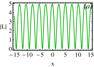
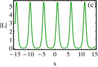
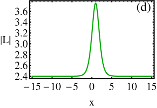
Figure 2: Plots of long wave component corresponding to the short wave components given in Fig. 2.

In Fig. 2, we have plotted the profiles of the long wave corresponding to the short waves shown in Fig. 1, in a clockwise manner. In Fig. 2((a)-(c)), one can observe periodic solitary waves. A localized anti-dark solitary wave structure is depicted in Fig. 2(d). This anti-dark structure results from the boundary condition $L\longrightarrow$ constant as $x\longrightarrow\pm\infty$. Such anti-dark solitons has been observed in (2+1) dimensional generalized nonlinear Schrödinger equation [30] and in cubic-quintic nonlinear Scrödinger equation [31]. All the parameters have the same values as in Fig. 1.

2.2 Solutions in terms of Lamé Polynomials of Order 2

In this sub-section, we present the periodic solutions of order 2 (l=2) of the (2+1) dimensional LSRI system (2). This case does not admit similar elliptic solutions. Here we obtain only mixed and superposed elliptic solutions which we present one by one.

2.2.1 Mixed elliptic solutions

We find there exist seven possible combinations of mixed elliptic solutions which are given below in Table 3.

Table 3: Mixed elliptic solutions of order 2

Mixed	$f_{1}(u)$	$f_{2}(u)$	Constraints on	Long wave
elliptic	$S_{1}=f_{1}$	$S_{2}=f_{2}\times$	parameters	component
solutions	$\times e^{-i(\omega_{1}t+\nu_{1}y-k_{1}x+\delta_{1})}$	$\times e^{-i(\omega_{2}t+\nu_{2}y-k_{2}x+\delta_{2})}$
(1)	$A~{}\sqrt{m}~{}\textit{{\rm cn}(u,m)}$ $\times\textit{{\rm dn}(u,m)}~{}$	$B~{}\sqrt{m}~{}\textit{{\rm sn}(u,m)}$ $\times\textit{{\rm dn}(u,m)}$	$v+\varepsilon_{1}w=2\delta k_{1}$,
			$~{}v+\varepsilon_{2}w=2\delta k_{2}$,
			$~{}c_{1}A^{2}=c_{2}B^{2}$,
			$\beta^{2}=-\delta\frac{\left(mc_{1}A^{2}\right)}{3v}>0$,	$\left(6\delta\beta^{2}\right){\rm dn}^{2}(u,m)$
			$\omega_{1}+\varepsilon_{1}\nu_{1}-\delta\left(k_{1}^{2}-(5-m)\beta^{2}\right)=0$,
			$\omega_{2}+\varepsilon_{2}\nu_{2}$
			$-\delta\left(k_{2}^{2}-(5-4m)\beta^{2}\right)=0$.

$$v+\varepsilon_{1}w=2\delta k_{1},~{}v+\varepsilon_{2}w=2\delta k_{2},~{}F=\pm A,~{}G=\pm B,~{}c_{1}A^{2}=-c_{2}B^{2},$$

$$~{}\beta^{2}=-\delta\frac{\left(2(p-q)c_{1}A^{2}\right)}{3\nu}>0,~{}p=\frac{D}{A},~{}q=\frac{E}{B},~{}p\neq q=-\frac{1}{12}[(5-m)\pm\sqrt{1+14m+m^{2}}],$$

$$~{}\omega_{1}+\varepsilon\nu_{1}-\delta\left(k_{1}^{2}-[5-m+3(3p+q)]\beta^{2}\right)=0,~{}\omega_{2}+\varepsilon\nu_{2}-\delta\left(k_{2}^{2}-[5-m+3(p+3q)]\beta^{2}\right)=0.$$ (12d)

Note that the signs of $F$ and $G$ are correlated, i.e. if $F=A~{}(F=-A)$ then $G=B~{}(G=-B)$.

2.2.3 Hyperbolic solutions $m=1$

The interesting hyperbolic solutions can be deduced by fixing the modulus parameter $m=1$ in the above second order elliptic function solutions. (a) The mixed solutions (1) and (2) of order 2 given in Table 3, reduce to the following hyperbolic form

$$S_{1} = \left[A~{}{\rm sech}^{2}(\beta(x-vt-wy+\delta_{0}))\right]~{}e^{-i(\omega_{1}t+\nu_{1}y-k_{1}x+\delta_{1})},$$ (13a)

$$S_{2} = \left[B~{}{\rm sech}(\beta(x-vt-wy+\delta_{0}))~{}\tanh(\beta(x-vt-wy+\delta_{0}))\right]~{}e^{-i(\omega_{2}t+\nu_{2}y-k_{2}x+\delta_{2})},$$ (13b)

$$L = \left(6\delta\beta^{2}\right){\rm sech}^{2}(\beta(x-vt-wy+\delta_{0})),$$ (13c)

along with the parametric restriction

$$v+\varepsilon_{1}w=2\delta k_{1},~{}v+\varepsilon_{2}w=2\delta k_{2},~{}c_{1}A^{2}=c_{2}B^{2},~{}\beta^{2}=-\delta\frac{c_{1}A^{2}}{3v}>0,$$

$$\omega_{1}+\varepsilon_{1}\nu_{1}-\delta\left(k_{1}^{2}-4\beta^{2}\right)=0,~{}\omega_{2}+\varepsilon_{2}\nu_{2}-\delta\left(k_{2}^{2}-\beta^{2}\right)=0.$$ (13d)

The above solitary wave solutions can be viewed as the blue-white-blue solutions reported in Ref. [18] for the three coupled nonlinear Schrödinger system. (b) It can be easily verified that the mixed solutions (3) and (4) of order 2 given in Table 3, either go over to above solutions (13) with $D=0$ or reduce to the hyperbolic solution

$$S_{1} = \left[A~{}{\rm sech}^{2}(\beta(x-vt-wy+\delta_{0}))~{}+D\right]~{}e^{-i(\omega_{1}t+\nu_{1}y-k_{1}x+\delta_{1})},$$ (14a)

$$S_{2} = \left[B~{}{\rm sech}(\beta(x-vt-wy+\delta_{0}))~{}\tanh(\beta(x-vt-wy+\delta_{0}))\right]~{}e^{-i(\omega_{2}t+\nu_{2}y-k_{2}x+\delta_{2})},$$ (14b)

$$L = \left(6\delta\beta^{2}\right){\rm sech}^{2}(\beta(x-vt-wy+\delta_{0}))-8~{}\delta~{}\beta^{2},$$ (14c)

along with the parametric restriction

$$v+\varepsilon_{1}w=2\delta k_{1},~{}v+\varepsilon_{2}w=2\delta k_{2},~{}~{}c_{1}A^{2}=c_{2}B^{2},~{}\beta^{2}=\delta\frac{\left(c_{1}A^{2}\right)}{9v}>0,$$

$$\omega_{1}+\varepsilon_{1}\nu_{1}-\delta\left(k_{1}^{2}+8\beta^{2}\right)=0,~{}\frac{D}{A}=p=-\frac{2}{3},~{}\omega_{2}+\varepsilon_{2}\nu_{2}-\delta\left(k_{2}^{2}+7\beta^{2}\right)=0.$$ (14d)

The above solitary wave solutions are similar to the red-white-red solutions discussed in Ref. [18] for the three coupled nonlinear Schrödinger system. But these solution behave different from that of Ref. [18] due to the constraint condition (14).

(c) The mixed elliptic solution (5) given in Table 3 takes the hyperbolic form given below:

$$S_{1} = \left[A~{}{\rm sech}^{2}(\beta(x-vt-uy+\delta_{0}))~{}+D\right]~{}e^{-i(\omega_{1}t+\nu_{1}y-k_{1}x+\delta_{1})},$$ (15a)

$$S_{2} = \left[B~{}{\rm sech}^{2}(\beta(x-vt-uy+\delta_{0}))\right]~{}e^{-i(\omega_{2}t+\nu_{2}y-k_{2}x+\delta_{2})},$$ (15b)

$$L = -\left(9\delta\beta^{2}\right)\left[p~{}{\rm sech}^{2}(\beta(x-vt-wy+\delta_{0}))+\frac{p^{2}}{2}\right],$$ (15c)

where the parameters are constrained by the following conditions:

$$v+\varepsilon_{1}w=2\delta k_{1},~{}v+\varepsilon_{2}w=2\delta k_{2},~{}\ ~{}c_{1}A^{2}=-c_{2}B^{2},~{}\beta^{2}=\delta\frac{\left(4c_{1}A^{2}\right)}{9v}>0,$$

$$\omega_{1}+\varepsilon_{1}\nu_{1}-\delta\left(k_{1}^{2}+2\beta^{2}\right)=0,~{}\frac{D}{A}=p=-\frac{2}{3},~{}\omega_{2}+\varepsilon_{2}\nu_{2}-\delta\left(k_{2}^{2}-2\beta^{2}\right)=0.$$ (15d)

This solution looks like red-blue-red solutions discussed in Ref. [18]. In the limit $m=1$, mixed elliptic solution (7) given in Table 3 and the superposed solution (LABEL:12) go over to solution (15), i.e., for these solutions $D\neq 0$, $E=0$ and rest of the solution is as given by (15). Needless to say, there is another solution similar to (15), i.e., in that case $E\neq 0$, $D=0$. Finally, in the limit $m=1$, the mixed elliptic solution (6) in Table 3 does not exist as $\beta^{2}$ becomes zero for this choice.

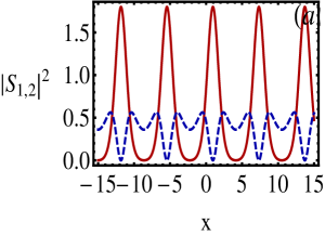
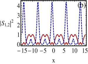
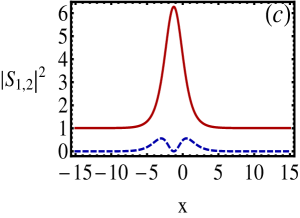
Figure 3: Red and dashed blue plots correspond to first and second components of short wave, respectively. (a) intensity plot of mixed elliptic solution (1) given in Table 3, for the choice $v=1.2$, $m=0.8$. (b) superposed solution given by Eq. (LABEL:12) for the choice $v=-0.5$, $m=0.8$ and for the condition $c_{1}=-c_{2}=1$. (c) intensity plot of anti-dark solitary wave solution in $S_{1}$ component and non-trivial bright bi-solitary wave solution in $S_{2}$ component given by Eqs. (14a) and (14b) for the choice $A=B$, $v=-1.0$, $m=1$. For Fig. 3(a) and Fig. 3(c) $c_{1}=c_{2}=1$. In all the figures, $y=0.5$, $t=1$, the parameters $A=1.5$, $\nu_{1}=\nu_{2}=1.2$, $w=1.5$, $\delta=-1$, $\varepsilon_{1,2}=1$, and $\delta_{0}=\delta_{1}=\delta_{2}=1$. In the case of $\delta=1$ also, we get same thing, so simply we present the $\delta=-1$ case only.

For illustrative purpose we have plotted some of the second order solutions in Fig. 3. In Fig. 3(a) the periodic waves given by mixed elliptic solution (1) in Table 3 is plotted. Here $S_{1}$ admits periodic solitary wave train and the $S_{2}$ admits doubly-periodic wave train. The superposed periodic waves given by Eq. (LABEL:12) are shown in Fig. 3(b). These superposed solutions show significant amplification in the pulse train. Finally, we have depicted the hyperbolic solutions given by Eqs. (14a) and (14b) in Fig.3(c). Here the first component ($S_{1}$) admits anti-dark solitary wave profile and the second component ($S_{2}$) has a bi-solitary wave profile.

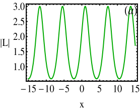
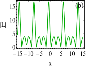
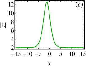
Figure 4: Intensity plots of long wave component corresponding to the short wave components given in Fig. (4).

Fig. 4(a) displays periodic solitary wave trains in the LW component (see solution 1 in Table 3) while Fig. 4(b) shows a doubly periodic wave train given by Eq. (13c). Fig. 4(c) shows an anti-dark solitary wave like structure given by Eq. (14c). One can verify that (15c) also admits such anti-dark solitary wave.

3 Jacobi Elliptic function solutions of the (1+1)-Dimensional two component LSRI system

In this section, we construct the Jacobi elliptic solution for (1+1) dimensional two component LSRI system (1). We can follow the same mathematical treatment as in the case of (2+1) dimensional case. Here also, we choose the travelling wave ansatz.

$$S_{j}=f_{j}[\beta(x-vt+\delta_{0})]e^{-i(\omega_{j}t-kx+\delta_{j})},\quad\quad j=1,2,$$ (16)

to construct the elliptic function solution of Eq. (1a). Here $f_{j}$ are real functions of $x$ and $t$; $\beta$, $\delta_{0}$ and $\delta_{1,2}$ are arbitrary real constants, $\omega_{j}$ is the frequency of the $j^{th}$ SW component, $k$ is the wave number and $v$ is the velocity of the short wave. Note that both the short waves are travelling with same velocity.

By substituting the above ansatz (16) into Eq. (1b), we obtain the LW component as

$$L=\frac{-2}{v}(c_{1}|S_{1}|^{2}+c_{2}|S_{2}|^{2}).$$ (17)

Substitution of the ansatz (16) in (1a) and using (17) result in a set of complex equations. On equating real and imaginary parts of the complex equations we respectively get

$$\frac{d^{2}f_{j}}{du^{2}}+\left[\frac{\delta\omega_{j}-k^{2}}{\beta^{2}}-\frac{2\delta}{v\beta^{2}}\left(c_{1}f_{1}^{2}+c_{2}f_{2}^{2}\right)\right]f_{j}=0,\;\;\;j=1,2,$$ (18a)

$$v=2\delta k.\qquad\qquad\qquad\qquad\qquad\qquad$$ (18b)

Here $\delta=\pm 1$ and $u=\beta(x-vt+\delta_{0})$. Next, we assume the Lamé function ansatz for $f_{j}$, that is,

$$f_{j}=\rho_{j}\psi_{j}^{(l)},\quad\quad l,j=1,2,$$ (19)

where $\psi_{j}^{(l)}$ is the first (second) order Lamé polynomials for $l=1$ ($l=2$), and satisfies the Lamé equation (7).

3.1 Solutions in terms of Lamé polynomials

As in the (2+1) dimensional case, here also we obtain similar, mixed, superposed elliptic solution of order one and mixed as well as superposed solutions of order two. For brevity, we mention how to write these solutions from their (2+1) dimensional counterparts. The first order solutions for the similar and mixed cases will be the same as given in Tables 1 and 2 while the second order mixed solutions will be similar to those given in Table 3 with $\varepsilon_{1}=\varepsilon_{2}=\nu_{1}=\nu_{2}=0$, $k_{1}=k_{2}=k$. Here one has to consider the corresponding constraint with this choice for a given pair of elliptic function solutions. For example, for this choice the similar elliptic solution (1) presented in Table 1 becomes;

$$S_{1} = A~{}{\rm dn}(u,m)e^{-i(\omega_{1}-kx+\delta_{1})},$$ (20a)

$$S_{2} = B~{}{\rm dn}(u,m)e^{-i(\omega_{2}-kx+\delta_{2})},$$ (20b)

$$L = \left[\left(2\delta\beta^{2}\right){\rm dn}^{2}(u,m)\right],$$ (20c)

where $$u=\beta(x-vt+\delta_{0})$$, with the parametric restriction

$$v=2\delta k,~{}\beta^{2}=-\delta\frac{\left(c_{1}A^{2}+c_{2}B^{2}\right)}{v}>0,~{}\omega_{1}=\delta\left[k^{2}-(2-m)\beta^{2}\right],~{}\omega_{2}=\omega_{1}.$$ (20d)

In a similar way all the first and second order solutions can be written. Similarly the first and second order superposed elliptic solutions and hyperbolic solutions also can be written from the corresponding two dimensional solutions by restricting the parameters as $\varepsilon_{1}=\varepsilon_{2}=\nu_{1}=\nu_{2}=0$, $k_{1}=k_{2}=k$. The associated constraint conditions also have to be rewritten appropriately with the above choice of parameters.

Figure 5: Red and dashed blue plots correspond to first and second components of short wave, respectively. (a) intensity plot of similar elliptic solution (1) given in Table 1, for the velocity value $v=1.2$, $m=0.8$. (b) intensity plot of mixed elliptic solution (2) given in Table 2, for the velocity value $v=0.2$, $m=0.8$. (c) superposed solution given by Eq. (8) for the velocity value $v=1.2$, $m=0.8$ and for the condition $A=D$, $B=E$. (d) plot of dark-dark solitary wave solution given by Eqs. (11a) and (11b) for the velocity value $A=1.2$, $B=1.2$, $v=1.2$, $m=1$. In all the figures, $y=0$, $t=1$, the parameters $A=1.5$ (except the Fig. 5(c)), $B=1.2$, $\nu_{1}=\nu_{2}=0$, $w=0$, $\delta=-1$, $\varepsilon_{1,2}=0$, $\delta_{0}=\delta_{1}=\delta_{2}=c_{1}=c_{2}=1$.

For illustrative purpose,we present some of the intensity plots of elliptic and hyperbolic solutions of the short wave components in Fig. 5. Here, Fig. 5(a) shows the periodic solution given by the similar solution (1) in Table 1, with the choice of parameters $\varepsilon_{1}=\varepsilon_{2}=\nu_{1}=\nu_{2}=0$, $k_{1}=k_{2}=k$. Fig. 5(b) shows the intensity plot of the mixed elliptic solution (2) given in Table 2, with the same above choice of parameters. It can be observed from the Fig. 5(a) and Fig. 5(b) that associated SW solutions are in-phase and out-of-phase. Then, superposed periodic wave solutions for the short wave components given by Eqs. (8a) and (8b) with the choice of parameters $\varepsilon_{1}=\varepsilon_{2}=\nu_{1}=\nu_{2}=0$, $k_{1}=k_{2}=k$ are plotted in Fig. 5(c). Finally, Fig. 5(d), depicts hyperbolic (dark-dark soliton) solution given by Eqs. (11a) and (11b) for the same above choice of parameters $\varepsilon_{1}=\varepsilon_{2}=\nu_{1}=\nu_{2}=0$, $k_{1}=k_{2}=k$. Here the first and second SW components are comprised of dark solitary waves.

Figure 6: Figures. 6((a)-(d)) depict the long wave component corresponding to the short wave components given in Figure. 5((a)-(d)), respectively.

In Fig. 6, we have plotted the profiles of the long wave corresponding to the short waves shown in Fig. 5. All the arbitrary parameters are same as in Fig. 5. Interestingly, in Fig. 5(d) corresponding to the solution given by Eq. (11c) with choice of parameters $\varepsilon_{1}=\varepsilon_{2}=\nu_{1}=\nu_{2}=0$, $k_{1}=k_{2}=k$, we observe a grey W type solitary wave.

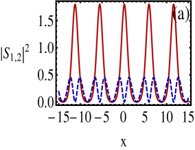
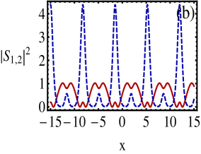
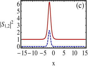
Figure 7: Red and dashed blue plots correspond to first and second components of short wave, respectively. (a) intensity plot of mixed elliptic solution (2) given in Table 3, for the choice $v=1.2$, $m=0.8$. (b) superposed solution given by Eq. (LABEL:12) for the choice $v=-0.5$, $m=0.8$ and for the condition $c_{1}=-c_{2}=1$. (c) intensity plot of anti-dark solitary wave solution in $S_{1}$ component and regular bright-solitary wave solution in $S_{2}$ component given by Eqs. (15a) and (15b) for the choice $A=B$, $v=-1.0$, $m=1$. For Fig. 3(a) and Fig. 3(c) $c_{1}=c_{2}=1$. In all the figures, $y=0$, $t=1$, the parameters $A=1.5$, $\nu_{1}=\nu_{2}=0$, $w=0$, $\delta=-1$, $\varepsilon_{1,2}=0$, and $\delta_{0}=\delta_{1}=\delta_{2}=1$. In the case of $\delta=1$ also, we get same thing, so simply we present the $\delta=-1$ case only.

Fig. 7(a) shows the periodic waves given by the second order mixed solution (2) in Table 3 with the choice of parameters $\varepsilon_{1}=\varepsilon_{2}=\nu_{1}=\nu_{2}=0$, $k_{1}=k_{2}=k$. Here the periodic wave train for the second component $S_{2}$ is intricate and it attains one minimum intensity when the other component $S_{1}$ reaches the maximum, while it reaches the second minimum exactly at the minimum of the second component $S_{2}$. Fig. 7(b) depicts the superposed periodic wave given by Eq. (LABEL:12) with the same choice of above parameters, but with significant compression in their widths and amplification in their amplitudes. Finally, in Fig. 7(c) we have depicted the hyperbolic solutions given by Eq. (15) with the choice of parameters $\varepsilon_{1}=\varepsilon_{2}=\nu_{1}=\nu_{2}=0$, $k_{1}=k_{2}=k$. Here the first component ($S_{1}$) is comprised of anti-dark solitary wave while the second component ($S_{2}$) admits standard bright solitary wave.

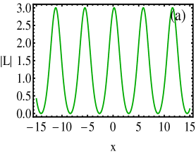
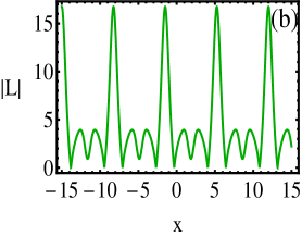
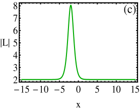
Figure 8: Plots of long wave component corresponding to the short wave components given in Fig. 7.

In Fig. 8, we have plotted the profile of the long wave corresponding to the short waves shown in Fig. 7. All the arbitrary parameters are same as in Fig. 7.

4 Conclusion

To conclude, first we obtain the Jacobi elliptic function solutions of two component (2+1) dimensional LSRI system (2) in terms of Lamé polynomials of order 1 and 2. We classified the solutions as similar, mixed and superposed elliptic waves based on their wave profile in the two SW components. We have reported special in-phase and out-of phase periodic wave train solutions. The similar elliptic solutions do not exist for the second order solutions. By considering the hyperbolic limit, we have identified anti-dark and double-hump solitary waves in the SW component with an anti-dark solitary wave like structure in the LW component. Then we extend the same mathematical treatment to the (1+1) dimensional two component LSRI system and constructed order-1 and order-2 elliptic waves. We have demonstrated that the SW components as well as LW component support rich profile structures like bright, dark, anti-dark and grey W type solitary waves. It is of future interest to generalize this study to M-component LSRI system with $M>2$. There are several other coupled systems [32]-[36] and higher dimensional systems [37] for which such elliptic wave solutions can be constructed. It will also be an interesting further work to numerically study the non-integrable versions of Eqs. (1) and (2) by making use of the elliptic function solutions as well as hyperbolic solutions reported here.

ACKNOWLEDGMENTS

The author AK acknowledges Department of Atomic Energy (DAE). Govt. of India for the financial support through Raja Ramanna Fellowship. The authors TK and KT acknowledge the Principal and Management of Bishop Heber College, Tiruchirapalli, for constant support and encouragement.

References

- [1] Whitham G B, 1999 Linear and Nonlinear Waves John Wiley, New York
- [2] Zakharov V E, 1972 Collapse of Langmuir waves Zh. Eksp. Teor. Fiz 35 908
- [3] Yajima N, Oikawa M, 1976 Formation and Interaction of Sonic-Langmuir Solitons Prog. Theor. Phys 56 1719
- [4] Benny D J, 1976 Significant interactions between small and large scale surface waves Stud. Appl. Phys 55 93; 1977 A general theory for interactions between short and long waves Stud. Appl. Phys 56 81
- [5] Kopp C G, Redekopp L G, 1981 The interation of long and short internal gravity waves: Theory and experiments J. Fluid Mech 111 367
- [6] Funakoshi M, Oikawa M, 1983 The resonant interaction between a long internal gravity wave and a surface gravity wave packet J. Phys. Soc.Jpn 52 1982
- [7] Oikawa M, Okamura M, Funakoshi M, 1989 Two-Dimensional Resonant Interaction between Long and Short Waves J. Phys. Soc.Jpn 58 4416
- [8] Kanna T, Sakkaravarthi K, Tamilselvan K, 2013 General multicomponent Yajima-Oikawa system: Painlevé analysis, soliton solutions, and energy-sharing collisions Phys. Rev. E 88 062921
- [9] Sazonov S V, Ustinov N V, 2011 Vector solitons generated by the long-wave–short-wave interaction JETP Lett. 94 610
- [10] Myrzakulov R, Pashaev O K, Kholmurodov Kh T, 1986 Particle-Like Excitations in Many Component Magnon-Phonon Systems Phys. Scr. 33 378
- [11] Chen S, Grelu P, Soto-Crespo J M, 2014 Dark- and bright-rogue-wave solutions for media with long-wave–short-wave resonance Phys. Rev. E 89 011201(R)
- [12] Ohta Y, Maruno K, Oikawa M, 2007 Two-component analogue of two-dimensional long-wave–short-wave resonance interaction equations: a derivation and solutions J. Phys. A:Math.Theor. 40 7659.
- [13] Kanna T, Vijayajayanthi M, Lakshmanan M, 2012 Mixed solitons in (2+1) dimensional multicomponent long-wave–short-wave system arXiv:1212.0097[nlin.SI](2012).
- [14] Onorato M, Osborne A R, Serio M, 2006 Modulational Instability in Crossing Sea States: A Possible Mechanism for the Formation of Freak Waves Phys. Rev. Lett. 96 014503
- [15] Shukla P K, Kourakis I, Eliasson B, Marklund M, Stenflo L, 2006 Instability and Evolution of Nonlinearly Interacting Water Waves Phys. Rev. Lett. 97 094501
- [16] Kanna T, Vijayajayanthi M, Sakkaravarthi K, Lakshmanan M, 2009 Higher dimensional bright solitons and their collisions in a multicomponent long wave–short wave system J. Phys. A: Math. Theor. 42 115103
- [17] Chow K W, Nakkeeran K, Malomed B A, 2003 Periodic waves in bimodal fibers Opt. Commun. 219 251
- [18] Hioe F T, 1998 Solitary waves for two and three coupled nonlinear Schrödinger equations Phys. Rev. E 58 6700
- [19] Hioe F T, Slater J S, 2002 Special set and solutions of coupled nonlinear Schrödinger equations J. Phys. A 35 8913
- [20] Hioe F T, 2002 N coupled nonlinear Schrödinger equations:Special set and applications to N=3 J. Math. Phys.43 6325
- [21] Hioe F T, 2002 N coupled nonlinear Schrödinger equations with mixed nonlinear interactions Phys. Lett. A 304 30
- [22] Chow K W, Lai D W C, 2003 Periodic solutions for systems of coupled nonlinear Schrödinger equations with three and four components Phys. Rev. E 68 017601
- [23] Chow K W, Lai D W C, 2002 Periodic solutions for systems of coupled nonlinear Schrödinger equations with five and six components Phys. Rev. E 65 026613
- [24] Florjanczyk M, Tremblay R, 1989 Periodic and solitary waves in bimodal optical fibers Phys. Lett. A 141 34
- [25] Petnikova V M, Shuvalov V V, Vysloukh V A, 1999 Multicomponent photorefractive cnoidal waves: stability, localization and soliton asymptotics Phys. Rev. E 60 1009
- [26] Wright III O C, 2013 On elliptic solutions of a coupled nonlinear Schrödinger system Phys. D 264 1-16
- [27] Whittaker E T, Watson G N, 1886 A course of modern analysis Cambridge University Press, London
- [28] Abramowitz M, Stegun I A, 1964 Handbook of mathematical functions: with formulas, graphs, and mathematical tables Dover Publications, USA; Gradshteyn I S, Ryzhik I M, 1980 Table of Integrals, Series and Products Academic Press, Boston
- [29] Khare A, Saxena A, 2013 Linear superposition for large number of nonlinear equations Phys. Lett. A 377 2761; 2014 Superposition of elliptic functions as solution of large number of nonlinear equations J. Math. Phys. 55 032701
- [30] Nistazakis, H E, Frantzeskakis D J, Balourdos P S, Tsigopoulos A, Malomed B A, 2000 Dynamics of anti-dark and dark solitons in (2+1)-dimensional generalized nonlinear Schrödinger equation Phys. Lett. A 278 68-76
- [31] Crosta M, Fratalocchi A, Trillo S, 2011 Bistability and instability of dark-antidark solitons in the cubic-quintic nonlinear Schrödinger equation Phys. Rev. A 84 063809
- [32] Zuo D W, Gao Y T, Meng G Q, Shen Y J, Yu X, 2014 Multi-soliton solutions for the three-coupled KdV equations engendered by the Neumann system 75 701–708
- [33] Kanna T, Vijayajayanthi M, Lakshmanan M, 2010 Coherently coupled bright optical solitons and their collisions J. Phys. A: Math. Theor. 43 434018
- [34] Wang Y F, Tian B, Li M, Wang P, Wang M, 2014 Integrability and soliton-like solutions for the coupled higher-order nonlinear Schrödinger equations with variable coefficients in inhomogeneous optical fibers Commun. Nonlinear Sci. Numer. Simul. 19 1783-1791
- [35] Wang D S,Zhang D J, Yang J, 2010 Integrable properties of the general coupled nonlinear Schrödinger equations J. Math. Phys. 51 023510
- [36] Kanna T, Babu Mareeswaran R, Sakkaravarthi K, 2014 Non-autonomous bright matter wave solitons in spinor Bose-Einstein condensates Phys. Lett. A 378 158-170
- [37] Zhen H L, Tian B, Wang Y F, Zhong H, Sun W R, 2014 Dynamic behavior of the quantum Zakharov-Kuznetsov equations in dense quantum magnetoplasmas Phys. Plasmas 21 012304