Spectator Scattering and Annihilation Contributions
as a Solution to the ${\pi}K$ and ${\pi}{\pi}$ Puzzles
within QCD Factorization Approach

Abstract

The large branching ratios for pure annihilation $\bar{B}_{s}^{0}$ $\to$ $\pi^{+}\pi^{-}$ and $\bar{B}_{d}^{0}$ $\to$ $K^{+}K^{-}$ decays reported by CDF and LHCb collaborations recently and the so-called ${\pi}K$ and ${\pi}{\pi}$ puzzles indicate that spectator scattering and annihilation contributions are important to the penguin-dominated, color-suppressed tree dominated, and pure annihilation nonleptonic $B$ decays. Combining the available experimental data for $B_{u,d}$ ${\to}$ $\pi\pi$, ${\pi}K$ and $K\bar{K}$ decays, we do a global fit on the spectator scattering and annihilation parameters $X_{H}({\rho}_{H}$, ${\phi}_{H})$, $X_{A}^{i}({\rho}_{A}^{i},{\phi}_{A}^{i})$ and $X_{A}^{f}({\rho}_{A}^{f},{\phi}_{A}^{f})$, which are used to parameterize the endpoint singularity in amplitudes of spectator scattering, nonfactorizable and factorizable annihilation topologies within the QCD factorization framework, in three scenarios for different purpose. Numerically, in scenario II, we get $({\rho}_{A}^{i},{\phi}_{A}^{i}[^{\circ}])=(2.88^{+1.52}_{-1.30},-103^{+33}_{-40})$ and $({\rho}_{A}^{f},{\phi}_{A}^{f}[^{\circ}])=(1.21^{+0.22}_{-0.25},-40^{+12}_{-8})$ at the $68\%$ confidence level, which are mainly demanded by resolving ${\pi}K$ puzzle and confirm the presupposition that $X_{A}^{i}\neq X_{A}^{f}$. In addition, correspondingly, the $B$-meson wave function parameter $\lambda_{B}$ is also fitted to be $0.18^{+0.11}_{-0.08}\,MeV$, which plays an important role for resolving both ${\pi}K$ and $\pi\pi$ puzzles. With the fitted parameters, the QCDF results for observables of $B_{u,d}$ $\to$ $\pi\pi$, $\pi K$ and $K\bar{K}$ decays are in good agreement with experimental measurements. Much more experimental and theoretical efforts are expected to understand the underlying QCD dynamics of spectator scattering and annihilation contributions.

I Introduction

Charmless hadronic $B$-meson decays provide a fertile ground for testing the Standard Model (SM) and exploring the source of $CP$ violation, which attract much attention in the past years. Thanks to the fruitful accomplishment of BABAR and Belle, the constraints on the sides and interior angles of the unitarity triangle significantly reduce the allowed ranges of some of the CKM elements, and many rare $B$ decays are well measured. With the successful running of LHC and the advent of Belle II at SuperKEKB, heavy flavour physics has entered a new exciting era and more $B$ decay modes will be measured precisely soon.

Recently, the evidence of pure annihilation decays $\bar{B}_{s}^{0}$ ${\to}$ ${\pi}^{+}{\pi}^{-}$ and $\bar{B}_{d}^{0}$ ${\to}$ $K^{+}K^{-}$ are firstly reported by CDF Collaboration CDFanni , and soon confirmed by LHCb Collaboration LHCbanni . The Heavy Flavor Averaging Group (HFAG) presents their branching ratios HFAG

$${\cal B}(\bar{B}_{s}^{0}{\to}{\pi}^{+}{\pi}^{-})=(0.73{\pm}0.14){\times}10^{-6},$$ (1)

$${\cal B}(\bar{B}_{d}^{0}{\to}K^{+}K^{-})=(0.12{\pm}0.05){\times}10^{-6}.$$ (2)

Such results, if confirmed, imply unexpectedly large annihilation contributions in $B$ decays and significant flavour symmetry breaking effects between the annihilation amplitudes of $B_{u,d}$ and $B_{s}$ decays, which attract much attention recently, for instance Refs. zhu1 ; zhu2 ; chang1 ; xiao1 .

Theoretically, as noticed already in Refs. pqcd ; relaRef ; du1 ; Beneke2 , even though the annihilation contributions are formally $\Lambda_{QCD}/m_{b}$ power suppressed, they are very important and indispensable for charmless $B$ decays. By introducing the parton transverse momentum and the Sudakov factor to regulate the endpoint divergence, there is a large complex annihilation contribution within the perturbative QCD (pQCD) approach pqcd ; relaRef . The latest renewed pQCD estimations ${\cal B}(\bar{B}_{s}^{0}\to\pi^{+}\pi^{-})$ $=$ $(5.10^{+1.96+0.25+1.05+0.29}_{-1.68-0.19-0.83-0.20})\times 10^{-7}$ and ${\cal B}(\bar{B}_{d}^{0}\to K^{+}K^{-})$ $=$ $(1.56^{+0.44+0.23+0.22+0.13}_{-0.42-0.22-0.19-0.09})\times 10^{-7}$ xiao1 give an appropriate account of the CDF and LHCb measurements within uncertainties. In the QCD factorization (QCDF) framework Beneke1 , the endpoint divergence in annihilation amplitudes is usually parameterized by $X_{A}(\rho_{A},\phi_{A})$ (see Eq.(9)). The parameters $\rho_{A}$ $\sim$ $1$ and $\phi_{A}$ $\sim$ $-55^{\circ}$ (scenario S4) Beneke2 are adopted conservatively in evaluating the amplitudes of $B$ $\to$ $PP$ decays, which lead to the predictions ${\cal B}(\bar{B}_{s}^{0}\to\pi^{+}\pi^{-})$ $=$ $(0.26^{+0.00+0.10}_{-0.00-0.09})\times 10^{-6}$ and ${\cal B}(\bar{B}_{d}^{0}\to K^{+}K^{-})$ $=$ $(0.10^{+0.03+0.03}_{-0.02-0.03})\times 10^{-6}$ Cheng2 . It is obvious that the QCDF prediction of ${\cal B}(\bar{B}_{d}^{0}\to K^{+}K^{-})$ agrees well with the data Eq.(2), but the one of ${\cal B}(\bar{B}_{s}^{0}\to\pi^{+}\pi^{-})$ is much smaller than the present experimental measurement Eq.(1). This discrepancy kindles the passions of restudy on annihilation contributions zhu1 ; zhu2 ; chang1 .

At present, there are two major issues among the well-concerning focus on the annihilation contributions within the QCDF framework, one is whether $X_{A}(\rho_{A},\phi_{A})$ is universal for $B$ decays, and the other is what its value should be. As to the first issue, there is no an imperative reason for the annihilation parameters $\rho_{A}$ and $\phi_{A}$ to be the same for different $B_{u,d,s}$ decays, even for different annihilation topologies, although they were usually taken to be universal in the previous numerical calculation for simplicity du1 ; Beneke2 . Phenomenologically, it is almost impossible to account for all of the well-measured two-body charmless $B$ decays with the universal values of $\rho_{A}$ and $\phi_{A}$ based on the QCDF approach zhu2 ; chang1 ; Beneke2 ; Cheng2 . In addition, the pQCD study on $B$ meson decays also indicate that the annihilation parameters $\rho_{A}$ and $\phi_{A}$ should be process-dependent. In fact, in the practical QCDF application to the $B$ ${\to}$ $PP$, $PV$ decays (where $P$ and $V$ denote the light pseudoscalar and vector $SU(3)$ meson nonet, respectively), the non-universal values of annihilation phase $\phi_{A}$ with respect to PP and PV final states are favored (scenario S4) Beneke2 ; the process-dependent values of $\rho_{A}$ and $\phi_{A}$ are given based on an educated guess Cheng2 ; Cheng1 or the comparison with the updated measurements chang1 ; the flavour-dependent values of $\rho_{A}$ and $\phi_{A}$ are suggested recently in the nonfactorizable annihilation contributions zhu2 . In principle the value of $\rho_{A}$ and $\phi_{A}$ should differ from each other for different topologies with different flavours, but we hope that the QCDF approach can accommodate and predict much more hadronic $B$ decays with less input parameters. So much attention in phenomenological analysis on the weak annihilation $B$ decays is devoted to what the appropriate values of the parameters $\rho_{A}$ and $\phi_{A}$ should be. This is the second issue. In principle, a large value of $\rho_{A}$ is unexpected by the power counting rules and the self-consistency validation within the QCDF framework. The original proposal is that $\rho_{A}$ ${\leq}$ $1$ and an arbitrary strong interaction phase $\phi_{A}$ are universal for all decay processes, and that a fine-tuning of the phase $\phi_{A}$ is required to be reconciled with experimental data when $\rho_{A}$ is significantly larger than 1 Beneke2 . The recent study on the annihilation contributions show that $\rho_{A}$ $>$ $2$ and ${|}\phi_{A}{|}$ $\geq$ $30^{\circ}$ are acceptable, even necessary, to reproduce the data for some two-body nonleptonic $B_{u,d,s}$ decay modes zhu2 ; chang1 . In this paper, we will perform a fitting on the parameters $\rho_{A}$ and $\phi_{A}$ by considering $B$ ${\to}$ ${\pi}{\pi}$, ${\pi}K$ and $K\bar{K}$ decay modes, on one hand, to investigate the strength of annihilation contribution, on the other hand, to study their effects on the anomalies in $B$ physics, such as the well-known ${\pi}K$ and ${\pi}{\pi}$ puzzles.

The so-called ${\pi}K$ puzzle is reflected by the difference between the direct $CP$ asymmetries for $B^{-}$ ${\to}$ $K^{-}\pi^{0}$ and $\bar{B}^{0}$ ${\to}$ $K^{-}\pi^{+}$ decays. With the up-to-date HFAG results HFAG , we get

$$\Delta A\equiv A_{CP}(B^{-}{\to}K^{-}{\pi}^{0})-A_{CP}(\bar{B}^{0}\to K^{-}\pi^{+})=(12.2\pm 2.2)\%,$$ (3)

which differs from zero by about $5.5\sigma$. However, the direct $CP$ asymmetries of $A_{CP}(B^{-}\to K^{-}\pi^{0})$ and $A_{CP}(\bar{B}^{0}\to K^{-}\pi^{+})$ are expected to be approximately equal with the isospin symmetry in the SM, numerically for instance $\Delta A\sim 0.5\%$ in the S4 scenario of QCDF Beneke2 .

The so-called ${\pi}{\pi}$ puzzle is reflected by the following two ratios of the $CP$-averaged branching fractions pipipuz :

$$R_{+-}^{\pi\pi}\equiv 2\Big{[}\frac{{\cal B}(B^{-}\to\pi^{-}\pi^{0})}{{\cal B}(\bar{B}^{0}\to\pi^{+}\pi^{-})}\Big{]}\frac{\tau_{B^{0}}}{\tau_{B^{+}}},\qquad R_{00}^{\pi\pi}\equiv 2\Big{[}\frac{{\cal B}(\bar{B}^{0}\to\pi^{0}\pi^{0})}{{\cal B}(\bar{B}^{0}\to\pi^{+}\pi^{-})}\Big{]}.$$ (4)

It is generally expected that branching ratio ${\cal B}(\bar{B}^{0}\to\pi^{+}\pi^{-})\gtrsim{\cal B}(B^{-}\to\pi^{-}\pi^{0})$ and ${\cal B}(\bar{B}^{0}\to\pi^{+}\pi^{-})\gg{\cal B}(\bar{B}^{0}\to\pi^{0}\pi^{0})$ within the SM. To date, the agreement of $R_{+-}^{\pi\pi}$ between the S4 scenario QCDF $R_{+-}^{\pi\pi}(\text{QCDF})$ $=$ $1.83$ Beneke2 and the refined experimental data $R_{+-}^{\pi\pi}(\text{Exp.})$ $=$ $1.99\pm 0.15$ HFAG can be achieved consistently within experimental error, while the discrepancy in $R_{00}^{\pi\pi}$ between the S4 scenario QCDF $R_{00}^{\pi\pi}(\text{QCDF})$ $=$ $0.27$ (where theoretical uncertainties are unenclosed) Beneke2 and the progressive experimental data $R_{+-}^{\pi\pi}(\text{Exp.})$ $=$ $1.99\pm 0.15$ HFAG is unexpectedly large.

It is claimed pipipuz that the so-called ${\pi}{\pi}$ puzzle could be accommodated by the nonfactorizable contributions in SM. It is argued Cheng1 ; pipipuz that to solve the so-called ${\pi}K$ puzzle, a large complex color-suppressed tree amplitude $C^{\prime}$ or a large complex electroweak penguin contribution $P_{\rm EW}^{\prime}$ or a combination of them are essential. An enhanced complex $P_{\rm EW}^{\prime}$ with a nontrivial strong phase can be obtained from new physics effects pipipuz . To get a large complex $C^{\prime}$, one can resort to spectator scattering and final state interactions Cheng1 ; Cheng2 . Recently, the annihilation amplitudes with large parameters $\rho_{A}$ is suggested to conciliate the recent measurements Eq.(1) and Eq.(2), so surprisingly, the ${\pi}K$ puzzle is also resolved simultaneously zhu2 . Theoretically, the power corrections, such as spectator scattering at the twist-3 order and annihilation amplitudes, are important to account for the large branching ratios and $CP$ asymmetries of penguin-dominated and/or color-suppressed tree-dominated $B$ decays. So, before claiming a new physics signal, it is essential to examine whether power corrections could retrieve “problematic” deviations from the SM expectations. Interestingly, our study show that with appropriate parameters, the annihilation and spectator scattering contributions could provide some possible solutions to the $\pi K$ and $\pi\pi$ puzzles.

Our paper is organized as following. In section II, we give a brief overview of the hard spectator and annihilation calculations and recent studies within QCDF. In section III, focusing on $\pi K$ and $\pi\pi$ puzzles, the effects of spectator scattering and annihilation contributions on $B$ $\to$ $\pi\pi$, $\pi K$ and $K\bar{K}$ decays are studied in detail in bluethree scenarios. In each scenario, a fitting on relevant parameters are performed. Our conclusions are summarized in section IV. Appendix A recapitulates the building blocks of annihilation and spectator scattering amplitudes. The input parameters and our fitting approach are given in Appendix B and C, respectively.

II Brief Review of Spectator Scattering and Annihilation Amplitudes within QCDF

The effective Hamiltonian for nonleptonic $B$ weak decays is Buchalla:1996vs

$${\cal H}_{\rm eff} = \frac{G_{F}}{\sqrt{2}}\sum\limits_{p,q}V_{pb}V_{pq}^{\ast}\Big{\{}\sum\limits_{i=1}^{10}C_{i}O_{i}+C_{7\gamma}O_{7\gamma}+C_{8g}O_{8g}\Big{\}}+{\rm h.c.},$$ (5)

where $V_{pb}V_{pq}^{\ast}$ ($p$ $=$ $u$, $c$ and $q$ $=$ $d$, $s$) is the product of the Cabibbo-Kobayashi-Maskawa (CKM) matrix elements; $C_{i}$ is the Wilson coefficient corresponding to the local four-quark operator $O_{i}$; $O_{7\gamma}$ and $O_{8g}$ are the electromagnetic and chromomagnetic dipole operators.

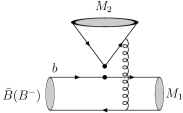
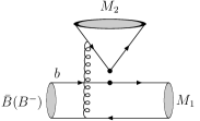
Figure 1: The lowest order diagrams of weak annihilation (a-d) and spectator scattering (e,f).

With the effective Hamiltonian Eq.(5), the QCDF method has been fully developed and extensively employed to calculate the hadronic two-body $B$ decays, for example, see du1 ; Beneke1 ; Beneke2 ; Cheng2 . The spectator scattering and annihilation amplitudes (see Fig.1) are expressed as the convolution of scattering functions with the light-cone wave functions of the participating mesons Beneke1 ; Beneke2 . The explicit expressions for the basic building blocks of spectator scattering and annihilation amplitudes have been given by Ref. Beneke2 , which are also listed in the appendix A for convenience. With the asymptotic light-cone distribution amplitudes, the building blocks for annihilation amplitudes of Eq.(34-38) could be simplified as Beneke2

$$A_{1}^{i} \simeq A_{2}^{i}\simeq 2\pi\alpha_{s}\Big{[}9\,\Big{(}X_{A}-4+\frac{\pi^{2}}{3}\Big{)}+r_{\chi}^{M_{1}}r_{\chi}^{M_{2}}X_{A}^{2}\Big{]},$$ (6)

$$A_{3}^{i} \simeq 6\pi\alpha_{s}\big{(}r_{\chi}^{M_{1}}-r_{\chi}^{M_{2}}\big{)}\Big{(}X_{A}^{2}-2X_{A}+\frac{\pi^{2}}{3}\Big{)},$$ (7)

$$A_{3}^{f} \simeq 6\pi\alpha_{s}(r_{\chi}^{M_{1}}+r_{\chi}^{M_{2}})(2X_{A}^{2}-X_{A}),$$ (8)

where the superscripts $i$ (or $f$) refers to gluon emission from the initial (or final) state quarks, respectively (see Fig.1). For the $\pi\pi$, $\pi K$ and $K\bar{K}$ final-state, $A_{3}^{i}$ is numerically negligible due to $r_{\chi}^{M_{1}}$ $\simeq$ $r_{\chi}^{M_{2}}$. The model-dependent parameter $X_{A}$ is used to estimate the endpoint contributions, and expressed as

$$\int_{0}^{1}\frac{dx}{x}\to X_{A}=(1+\rho_{A}e^{i\phi_{A}})\ln\frac{m_{B}}{\Lambda_{h}},$$ (9)

where $\Lambda_{h}$ $=$ $0.5$ GeV. For spectator scattering contributions, the calculation of twist-3 distribution amplitudes also suffers from endpoint divergence, which is usually dealt with the same manner as Eq.(9) and labelled by $X_{H}$ Beneke2 . Moreover, a quantity $\lambda_{B}$ is used to parameterize our ignorance about $B$-meson distribution amplitude [see Eq.(39)] through Beneke2

$$\int_{0}^{1}\frac{d\xi}{\xi}\Phi_{B}(\xi)\ \equiv\ \frac{m_{B}}{\lambda_{B}}.$$ (10)

The QCDF approach itself cannot give information or/and constraint on the phenomenological parameters of $X_{A}$, $X_{H}$ and ${\lambda_{B}}$. These parameters should be determined from experimental data. To conform with measurements of nonleptonic $B$ ${\to}$ $PP$ decays, we will adopt a similar method used in Ref.zhu2 to deal with the contributions from weak annihilation and spectator scattering. Focusing on the flavor dependence, without consideration of theoretical uncertainties, annihilation contributions are reevaluated in detail zhu2 to explain the ${\pi}K$ puzzle and the recent measurements on pure annihilation decays $\bar{B}_{s}^{0}$ ${\to}$ ${\pi}^{+}{\pi}^{-}$ and $\bar{B}_{d}^{0}$ ${\to}$ $K^{+}K^{-}$ [see Eq.(1,2)]. The authors of Ref. zhu2 find that the flavour symmetry breaking effects should be carefully considered for $B_{u,d,s}$ decays, and suggest that the parameters of $\rho_{A}$ and $\phi_{A}$ in nonfactorizable annihilation topologies $A^{i}_{k}$ [see Eq.(6,7)] should be different from those in factorizable annihilation topologies $A^{f}_{k}$ [see Eq.(8)]. (1) For factorizable annihilation topologies, i.e., the gluon emission from the final states Fig.1(c,d), the flavor symmetry breaking effects are embodied in the decay constants, because the asymptotic light-cone distribution amplitudes of final states are the same. In addition, all decay constants have been factorized outside from the hadronic matrix elements of factorizable annihilation topologies. So $A^{f}_{k}$ is independent of the initial state, and is the same for $B_{u,d,s}$ annihilation decays to two light pseudoscalar mesons, that is to say, $\rho^{f}_{A}$ and $\phi^{f}_{A}$ should be universal for $B_{u,d,s}$ $\to$ $PP$ decays. (2) For nonfactorizable annihilation topologies, i.e., the gluon emission from the initial $B$ meson Fig.1(a,b), besides the factorized decay constants and the same asymptotic light-cone distribution amplitudes, $B$ meson wave functions $\Phi_{B}(\xi)$ are involved in the convolution integrals of hadronic matrix elements. Hence, $A^{i}_{k}$ should depend on the initial state and be different for $B_{u,d}$ from $B_{s}$ meosn due to flavor symmetry breaking effects, i.e., parameters of $\rho^{i}_{A}$ and $\phi^{i}_{A}$ should be non-universal for $B_{s}$ and $B_{u,d}$ meson decays, and be different from parameters of $\rho^{f}_{A}$ and $\phi^{f}_{A}$ for $A^{f}_{k}$. In fact, the symmetry breaking effects have been considered in pervious QCDF study on two-body hadronic $B$ decays Cheng1 ; Cheng2 ; Cheng3 ; Beneke2 ; chang1 , but with parameters of $\rho^{f}_{A}$ $=$ $\rho^{i}_{A}$ and $\phi^{f}_{A}$ $=$ $\phi^{i}_{A}$. So, it is essential to systematically reevaluate factorizable and nonfactorizable annihilation contributions and preform a global fit on the annihilation parameters with the current available experimental data. In this paper, we will pay much attention to $B_{u,d}$ ${\to}$ $KK$, ${\pi}K$, ${\pi}{\pi}$ decays and the aforementioned ${\pi}K$, ${\pi}{\pi}$ puzzles with a distinction between ($\rho^{f}_{A}$, $\phi^{f}_{A}$) and ($\rho^{i}_{A}$, $\phi^{i}_{A}$), i.e., $X_{A}^{i}$ $\neq$ $X_{A}^{f}$.

As aforesaid Cheng1 ; pipipuz , the nonfactorizable spectator scattering amplitudes contribute to a large complex $C^{\prime}$, which is important to resolve the ${\pi}K$, ${\pi}{\pi}$ puzzles. From the building block Eq.(39), it can be easily seen that $B$ meson wave functions $\Phi_{B}(\xi)$ appear in the spectator scattering amplitudes. Therefore, the symmetry breaking effects should also be considered for the quantity $X_{H}$ that is introduced to parameterize the endpoint singularity in the twist-3 level spectator scattering corrections. Similar to $X_{A}^{i}$, the quantity $X_{H}$ is related to the topologies that gluon emit from the initial $B$ meson. So, for simplicity, the approximation $X_{H}$ $=$ $X_{A}^{i}$ is assumed in our coming numerical evaluation (scenarios I and II, see the next section for detail). Of course, this approximation is neither based on solid ground or from some underlying principle, and should be carefully studied and deserve much research. In fact, our coming phenomenological study (scenarios III) shows that the approximation $X_{H}$ $=$ $X_{A}^{i}$ is allowable with the up-to-date measurement on $B_{u,d}$ ${\to}$ $KK$, ${\pi}K$, ${\pi}{\pi}$ decays. In addition, it can be seen from Eq.(39) that the spectator scattering corrections depend strongly on the inverse moment parameter ${\lambda}_{B}$ given in Eq.(10). Recently, the value of ${\lambda}_{B}$ is an increasing concern of theoretical and experimental physicists Beneke5 ; Beneke4 ; Braun ; BaBarBA1 ; BaBarBA2 ; lambda . A scrutiny of parameter ${\lambda}_{B}$ becomes imperative. In this paper, we will give some information on ${\lambda}_{B}$ required by present experimental data of $B_{u,d}$ ${\to}$ $K\bar{K}$, ${\pi}K$, ${\pi}{\pi}$ decays.

III numerical analysis and discussions

With the conventions in Ref. Beneke2 , the decay amplitudes for $B_{u,d}$ ${\to}$ $\pi K$, $K\bar{K}$, $\pi\pi$ decays within the QCDF framework can be written as

$${\cal A}_{B^{-}\to\pi^{-}\bar{K}^{0}} = \sum\limits_{p=u,c}V_{pb}V_{ps}^{\ast}A_{\pi K}\Big{\{}\alpha_{4}^{p}-\frac{1}{2}\alpha_{4,{\rm EW}}^{p}+{\delta}_{pu}\beta_{2}+\beta_{3}^{p}+\beta_{3,{\rm EW}}^{p}\Big{\}},$$ (11)

$$\sqrt{2}{\cal A}_{B^{-}\to\pi^{0}K^{-}} = \sum\limits_{p=u,c}V_{pb}V_{ps}^{\ast}\Big{\{}A_{\pi K}\Big{[}\delta_{pu}(\alpha_{1}+\beta_{2})+\alpha_{4}^{p}+\alpha_{4,{\rm EW}}^{p}+\beta_{3}^{p}+\beta_{3,{\rm EW}}^{p}\Big{]}$$ (12)

$$+A_{K\pi}\Big{[}\delta_{pu}\alpha_{2}+\frac{3}{2}\alpha_{3,{\rm EW}}^{p}\Big{]}\Big{\}},$$

$${\cal A}_{\bar{B}^{0}\to\pi^{+}K^{-}} = \sum\limits_{p=u,c}V_{pb}V_{ps}^{\ast}A_{\pi K}\Big{\{}\delta_{pu}\alpha_{1}+\alpha_{4}^{p}+\alpha_{4,{\rm EW}}^{p}+\beta_{3}^{p}-\frac{1}{2}\beta_{3,{\rm EW}}^{p}\Big{\}},$$ (13)

$$\sqrt{2}{\cal A}_{\bar{B}^{0}\to\pi^{0}\bar{K}^{0}} = \sum\limits_{p=u,c}V_{pb}V_{ps}^{\ast}\Big{\{}A_{\pi K}\Big{[}-\alpha_{4}^{p}+\frac{1}{2}\alpha_{4,{\rm EW}}^{p}-\beta_{3}^{p}+\frac{1}{2}\beta_{3,{\rm EW}}^{p}\Big{]}$$ (14)

$$+A_{K\pi}\Big{[}\delta_{pu}\alpha_{2}+\frac{3}{2}\alpha_{3,{\rm EW}}^{p}\Big{]}\Big{\}},$$

$${\cal A}_{B^{-}\to K^{0}\bar{K}^{0}} = \sum\limits_{p=u,c}V_{pb}V_{pd}^{\ast}A_{KK}\Big{\{}\alpha_{4}^{p}-\frac{1}{2}\alpha_{4,{\rm EW}}^{p}+\delta_{pu}\beta_{2}+\beta_{3}^{p}+\beta_{3,{\rm EW}}^{p}\Big{\}},$$ (15)

$${\cal A}_{\bar{B}^{0}\to K^{-}K^{+}} = \sum\limits_{p=u,c}V_{pb}V_{pd}^{\ast}\Big{\{}B_{\bar{K}K}\Big{[}\delta_{pu}b_{1}+b_{4}^{p}+b_{4,{\rm EW}}^{p}\Big{]}+B_{K\bar{K}}\Big{[}b_{4}^{p}-\frac{1}{2}b_{4,{\rm EW}}^{p}\Big{]}\Big{\}},$$ (16)

$${\cal A}_{\bar{B}^{0}\to\bar{K}^{0}K^{0}} = \sum\limits_{p=u,c}V_{pb}V_{pd}^{\ast}\Big{\{}A_{\bar{K}K}\Big{[}\alpha_{4}^{p}-\frac{1}{2}\alpha_{4,{\rm EW}}^{p}+\beta_{3}^{p}+\beta_{4}^{p}-\frac{1}{2}\beta_{3,{\rm EW}}^{p}-\frac{1}{2}\beta_{4,{\rm EW}}^{p}\Big{]}$$ (17)

$$+B_{K\bar{K}}\Big{[}b_{4}^{p}-\frac{1}{2}b_{4,{\rm EW}}^{p}\Big{]}\Big{\}},$$

$$\sqrt{2}{\cal A}_{B^{-}\to\pi^{-}\pi^{0}} = \sum\limits_{p=u,c}V_{pb}V_{pd}^{\ast}A_{\pi\pi}\Big{\{}\delta_{pu}(\alpha_{1}+\alpha_{2})+\frac{3}{2}(\alpha_{3,{\rm EW}}^{p}+\alpha_{4,{\rm EW}}^{p})\Big{\}},$$ (18)

$${\cal A}_{\bar{B}^{0}\to\pi^{+}\pi^{-}} = \sum\limits_{p=u,c}V_{pb}V_{pd}^{\ast}A_{\pi\pi}\Big{\{}\delta_{pu}(\alpha_{1}+\beta_{1})+\alpha_{4}^{p}+\alpha_{4,{\rm EW}}^{p}+\beta_{3}^{p}+2\beta_{4}^{p}$$ (19)

$$-\frac{1}{2}\beta_{3,{\rm EW}}^{p}+\frac{1}{2}\beta_{4,{\rm EW}}^{p}\Big{\}},$$

$$-{\cal A}_{\bar{B}^{0}\to\pi^{0}\pi^{0}} = \sum\limits_{p=u,c}V_{pb}V_{pd}^{\ast}A_{\pi\pi}\Big{\{}\delta_{pu}(\alpha_{2}-\beta_{1})-\alpha_{4}^{p}+\frac{3}{2}\alpha_{3,{\rm EW}}^{p}+\frac{1}{2}\alpha_{4,{\rm EW}}^{p}$$ (20)

$$-\beta_{3}^{p}-2\beta_{4}^{p}+\frac{1}{2}\beta_{3,{\rm EW}}^{p}-\frac{1}{2}\beta_{4,{\rm EW}}^{p})\Big{\}}.$$

For the sake for convenient discussion, we reiterate the expressions of the annihilation coefficients Beneke2 ,

$${\beta}_{i}^{p} = b_{i}^{p}B_{M_{1}M_{2}}/A_{M_{1}M_{2}},$$ (21)

$$b_{1} = \frac{C_{F}}{N_{c}^{2}}\,C_{1}A_{1}^{i},\quad\quad\quad b_{2}=\frac{C_{F}}{N_{c}^{2}}\,C_{2}A_{1}^{i},$$ (22)

$$b_{3}^{p} = \frac{C_{F}}{N_{c}^{2}}\,\Big{[}C_{3}A_{1}^{i}+C_{5}(A_{3}^{i}+A_{3}^{f})+N_{c}C_{6}A_{3}^{f}\Big{]},$$ (23)

$$b_{4}^{p} = \frac{C_{F}}{N_{c}^{2}}\,\Big{[}C_{4}A_{1}^{i}+C_{6}A_{2}^{i}\Big{]},$$ (24)

$$b_{3,\rm EW}^{p} = \frac{C_{F}}{N_{c}^{2}}\,\Big{[}C_{9}A_{1}^{i}+C_{7}(A_{3}^{i}+A_{3}^{f})+N_{c}C_{8}A_{3}^{f}\Big{]},$$ (25)

$$b_{4,\rm EW}^{p} = \frac{C_{F}}{N_{c}^{2}}\,\Big{[}C_{10}A_{1}^{i}+C_{8}A_{2}^{i}\Big{]}.$$ (26)

Numerically, coefficients of $b_{3,\rm EW}^{p}$ and $b_{4,\rm EW}^{p}$ are negligible compared with the other effective coefficients due to the small electroweak Wilson coefficients, and so their effects would be not discussed in this paper.

In order to illustrate the contributions of annihilation and spectator scattering, we explore three parameter scenarios in which certain parameters are changed freely.

• Scenario I: $B_{u,d}$ ${\to}$ $\pi K$ and $K\bar{K}$ decays, including the $\pi K$ puzzle and pure annihilation decay $B_{d}$ $\to$ $K^{-}K^{+}$, are studied in detail. Combining the latest experimental data on the $CP$-averaged branching ratios, direct and mixing-induced $CP$-asymmetries, total 14 observables (see Table.2, 3, 4) for seven $B_{u,d}$ ${\to}$ $\pi K$, $K\bar{K}$ decay modes [see Eq.(11—17)], the fit on four parameters ($\rho^{f}_{A}$, $\phi^{f}_{A}$) and ($\rho^{i}_{A}$, $\phi^{i}_{A}$) is performed with the fixed value $\lambda_{B}$ $=$ 0.2 GeV and the approximation ($\rho_{H}$, $\phi_{H}$) = ($\rho^{i}_{A}$, $\phi^{i}_{A}$), where ($\rho^{f}_{A}$, $\phi^{f}_{A}$), ($\rho^{i}_{A}$, $\phi^{i}_{A}$) and ($\rho_{H}$, $\phi_{H}$) are assumed to be universal for factorizable annihilation amplitudes, nonfactorizable annihilation amplitudes and spectator scattering corrections, respectively.

• Scenario II: $B_{u,d}$ ${\to}$ $\pi K$, $K\bar{K}$ and $\pi\pi$ decays, including $\pi\pi$ puzzle, are studied. Combining the latest experimental data on the $CP$-averaged branching ratios, direct and mixing-induced $CP$-asymmetries, total 21 observables (see Table.2, 3, 4) for ten $B_{u,d}$ ${\to}$ $\pi K$, $K\bar{K}$, $\pi\pi$ decay modes [see Eq.(11—20)], the fit on five parameters ($\rho^{f}_{A}$, $\phi^{f}_{A}$), ($\rho^{i}_{A}$, $\phi^{i}_{A}$) and $\lambda_{B}$ is performed with the approximation ($\rho_{H}$, $\phi_{H}$) = ($\rho^{i}_{A}$, $\phi^{i}_{A}$).

• Scenario III: As a general scenario, to clarify the relative strength among ($\rho^{f}_{A}$, $\phi^{f}_{A}$), ($\rho^{i}_{A}$, $\phi^{i}_{A}$) and ($\rho_{H}$, $\phi_{H}$), and check whether the approximation ($\rho_{H}$, $\phi_{H}$) = ($\rho^{i}_{A}$, $\phi^{i}_{A}$) is allowed or not, a fit on such six free parameters is performed.

Other input parameters used in our evaluation are summarized in Appendix B. Our fit approach is illustrated in detail in Appendix C.

III.1 Scenario I

Comparing Eq.(12) with Eq.(13), it can be clearly seen that $\sqrt{2}{\cal A}_{B^{-}\to\pi^{0}K^{-}}$ $\simeq$ ${\cal A}_{\bar{B}^{0}\to\pi^{+}K^{-}}$ if $\delta_{pu}\alpha_{2}$ $+$ $\frac{3}{2}\alpha_{3,{\rm EW}}^{p}$ is negligible compared with $\delta_{pu}\alpha_{1}$ $+$ $\alpha_{4}^{p}$. Hence it is expected $\Delta A$ $\simeq$ 0 in SM, which significantly disagrees with the current experimental data in Eq.(3), this is the so-called $\pi K$ puzzle. To resolve the $\pi K$ puzzle, one possible solution is that there is a large complex contributions from $\delta_{pu}\alpha_{2}$ $+$ $\frac{3}{2}\alpha_{3,{\rm EW}}^{p}$. Many proposals have been offered, such as the enhancement of color-suppressed tree amplitude $\alpha_{2}$ in Ref.Cheng1 , significant new physics corrections to the electroweak penguin coefficient $\alpha_{3,{\rm EW}}^{p}$ in Ref.pipipuz , and so on. Indeed, it has been shown Beneke2 that the coefficients $\alpha_{2}$ and $\alpha_{3,{\rm EW}}^{p}$ are seriously affected by spectator scattering corrections within QCDF framework. Consequently, the nonfactorizable spectator scattering parameters $X_{H}$ or ($\rho_{H}$, $\phi_{H}$) will have great influence on the observable $\Delta A$. Furthermore, a scrutiny of difference between Eq.(12) and Eq.(13), another possible resolution to the $\pi K$ puzzle might be provided by annihilation contributions, such as coefficient $\beta_{2}$, as suggested in Ref.zhu2 . If so, then $\Delta A$ will depend strongly on the nonfactorizable annihilation parameters ($\rho_{A}^{i}$, $\phi_{A}^{i}$) because $\beta_{2}$ is proportional to $A_{1}^{i}$ in Eq.(22). Additionally, it can be seen from Eq.(12) and Eq.(13) that annihilation coefficient $\beta_{3}^{p}$ contributes to amplitudes both ${\cal A}_{B^{-}\to\pi^{0}K^{-}}$ and ${\cal A}_{\bar{B}^{0}\to\pi^{+}K^{-}}$. If $\beta_{3}^{p}$ could offer a large strong phase, then its effect should contribute to the direct $CP$ asymmetries $A_{CP}(B^{-}\to\pi^{0}K^{-})$ and $A_{CP}(\bar{B}^{0}\to\pi^{+}K^{-})$ rather than $\Delta A$. Due to the fact that the lion’s share of $\beta_{3}^{p}$ comes from $N_{c}C_{6}A_{3}^{f}$ in Eq.(23), the direct $CP$ asymmetries $A_{CP}(B^{-}\to\pi^{0}K^{-})$ and $A_{CP}(\bar{B}^{0}\to\pi^{+}K^{-})$ should vary greatly with the factorizable annihilation parameters $X_{A}^{f}$, while $\Delta A$ should be insensitive to variation of parameters ($\rho_{A}^{f}$, $\phi_{A}^{f}$). The above analysis and speculations are confirmed by Fig.2.

From Eq.(16), it is seen that the amplitude ${\cal A}_{\bar{B}^{0}\to K^{-}K^{+}}$ depends heavily on coefficients $\beta_{1}$ and $\beta_{4}^{p}$, which are closely associated with the nonfactorizable annihilation parameter $X_{A}^{i}$ only. The factorizable annihilation contributions vanish due to the isospin symmetry, which is consistent with the pQCD calculation xiao1 . The large branching ratio Eq.(2) would appeal for large nonfactorizable annihilation parameter $X_{A}^{i}$ or $\rho_{A}^{i}$. The dependence of branching ratio ${\cal B}(\bar{B}^{0}\to K^{-}K^{+})$ on the parameters ($\rho_{A}^{i}$, $\phi_{A}^{i}$) is displayed in Fig.3.

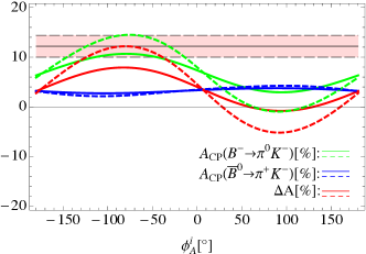
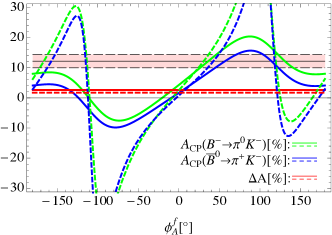
Figure 2: The direct $CP$ asymmetries $A_{CP}(B^{-}\to\pi^{0}K^{-})$, $A_{CP}(\bar{B}^{0}\to\pi^{+}K^{-})$ and their difference $\Delta A$ via (a) parameters ($\rho_{A}^{i}$, $\phi_{A}^{i}$) with $\rho_{A}^{f}$ $=$ $\phi_{A}^{f}$ $=$ $0$; and (b) parameters ($\rho_{A}^{f}$, $\phi_{A}^{f}$) with $\rho_{A}^{i}$ $=$ $\phi_{A}^{i}$ $=$ $0$, where the solid and dashed lines correspond to $\rho_{A}^{i,f}$ $=$ $1$ and $2$, respectively; The shaded band is the experimental result for $\Delta A$ with $1\sigma$ error.

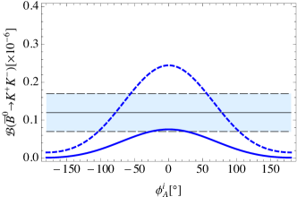
Figure 3: The dependence of branching ratio ${\cal B}(\bar{B}^{0}\to K^{-}K^{+})$ on nonfactorizable annihilation parameters ($\rho_{A}^{i}$, $\phi_{A}^{i}$). The notes are the same as Fig.2.

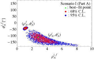
Figure 4: The allowed regions of annihilation parameters at $68\%$ C. L. and $95\%$ C. L. in $(\rho_{A}^{i,f},\phi_{A}^{i,f})$ planes, where the best-fit points of part A and B correspond to $\chi^{2}_{\rm min}$ $=$ $2.47$ and $\chi^{2}_{\rm min}$ $=$ $2.46$, respectively.

Table 1: Numerical results of annihilation parameters in scenario I.

	$\rho_{H}$ $=$ $\rho_{A}^{i}$	$\phi_{H}$ $=$ $\phi_{A}^{i}\,[^{\circ}]$	$\rho_{A}^{f}$	$\phi_{A}^{f}[^{\circ}]$
Part A	$2.82^{+2.73}_{-1.15}$	$-108^{+44}_{-50}$	$1.07^{+0.30}_{-0.20}$	$-40^{+10}_{-11}$
Part B	$2.86^{+2.68}_{-1.20}$	$-108^{+42}_{-51}$	$2.72^{+0.30}_{-0.22}$	$166^{+3}_{-4}$

Table 2: The CP-averaged branching ratios (in units of $10^{-6}$) of $B$ ${\to}$ $\pi K$, $K\bar{K}$, $\pi\pi$ decays. For the Part A results of scenario I and II, the first and second theoretical uncertainties are caused by the CKM and other input parameters, respectively.

Decay Mode	Exp. HFAG	scenario I	scenario II	S4 Beneke2
$B^{-}\to\pi^{-}\bar{K}^{0}$	$23.79\pm 0.75$	$20.53^{+1.52+4.28}_{-0.65-3.87}$	$21.54^{+1.60+4.40}_{-0.68-3.99}$	$20.3$
$B^{-}\to\pi^{0}K^{-}$	$12.94^{+0.52}_{-0.51}$	$11.29^{+0.88+2.14}_{-0.45-1.96}$	$11.78^{+0.92+2.20}_{-0.47-2.01}$	$11.7$
$\bar{B}^{0}\to\pi^{+}K^{-}$	$19.57^{+0.53}_{-0.52}$	$17.54^{+1.34+3.61}_{-0.65-3.27}$	$18.51^{+1.41+3.73}_{-0.67-3.38}$	$18.4$
$\bar{B}^{0}\to\pi^{0}\bar{K}^{0}$	$9.93\pm 0.49$	$8.05^{+0.60+1.84}_{-0.27-1.65}$	$8.60^{+0.65+1.90}_{-0.29-1.72}$	$8.0$
$B^{-}\to K^{-}K^{0}$	$1.19\pm 0.18$	$1.45^{+0.13+0.32}_{-0.09-0.29}$	$1.51^{+0.13+0.32}_{-0.09-0.29}$	$1.46$
$\bar{B}^{0}\to K^{-}K^{+}$	$0.12\pm 0.05$	$0.13^{+0.01+0.02}_{-0.01-0.02}$	$0.15^{+0.02+0.02}_{-0.01-0.02}$	$0.07$
$\bar{B}^{0}\to K^{0}\bar{K}^{0}$	$1.21\pm 0.16$	$1.22^{+0.11+0.27}_{-0.08-0.24}$	$1.32^{+0.12+0.27}_{-0.08-0.25}$	$1.58$
$B^{-}\to\pi^{-}\pi^{0}$	$5.48^{+0.35}_{-0.34}$	$5.20^{+0.64+1.11}_{-0.47-1.00}$	$5.59^{+0.68+1.15}_{-0.51-1.04}$	$5.1$
$\bar{B}^{0}\to\pi^{+}\pi^{-}$	$5.10\pm 0.19$	$5.88^{+0.66+1.66}_{-0.49-1.45}$	$5.74^{+0.64+1.63}_{-0.47-1.42}$	$5.2$
$\bar{B}^{0}\to\pi^{0}\pi^{0}$	$1.91^{+0.22}_{-0.23}$	$1.67^{+0.22+0.25}_{-0.19-0.23}$	$2.13^{+0.29+0.32}_{-0.24-0.29}$	$0.7$
$R_{+-}^{\pi\pi}$	$1.99\pm 0.15$	$1.64^{+0.06+0.13}_{-0.06-0.11}$	$1.80^{+0.07+0.17}_{-0.07-0.13}$	$1.82$
$R_{00}^{\pi\pi}$	$0.75\pm 0.09$	$0.57^{+0.06+0.16}_{-0.06-0.12}$	$0.74^{+0.08+0.22}_{-0.08-0.17}$	$0.27$

Table 3: The direct CP asymmetries (in units of $10^{-2}$) of $B$ ${\to}$ $\pi K$, $K\bar{K}$, $\pi\pi$ decays. The notes on uncertainties are the same as Table2.

Decay Mode	Exp. HFAG	scenario I	scenario II	S4 Beneke2
$B^{-}\to\pi^{-}\bar{K}^{0}$	$-1.5\pm 1.9$	$-0.05^{+0.00+0.13}_{-0.00-0.15}$	$-0.17^{+0.01+0.14}_{-0.01-0.15}$	$0.3$
$B^{-}\to\pi^{0}K^{-}$	$4.0\pm 2.1$	$3.2^{+0.2+0.6}_{-0.2-0.6}$	$2.5^{+0.1+0.6}_{-0.1-0.6}$	$-3.6$
$\bar{B}^{0}\to\pi^{+}K^{-}$	$-8.2\pm 0.6$	$-7.7^{+0.4+0.9}_{-0.4-0.9}$	$-9.1^{+0.4+0.9}_{-0.5-0.9}$	$-4.1$
$\bar{B}^{0}\to\pi^{0}\bar{K}^{0}$	$-1\pm 10$	$-10.3^{+0.6+0.9}_{-0.6-1.0}$	$-10.6^{+0.6+0.9}_{-0.6-0.9}$	$0.8$
$\Delta A$	$12.2\pm 2.2$	$10.9^{+0.6+0.9}_{-0.5-0.8}$	$11.6^{+0.6+0.9}_{-0.6-0.8}$	$0.5$
$B^{-}\to K^{-}K^{0}$	$3.9\pm 14.1$	$-0.6^{+0.0+3.2}_{-0.0-2.9}$	$2.0^{+0.1+3.4}_{-0.1-3.0}$	$-4.3$
$\bar{B}^{0}\to K^{0}\bar{K}^{0}$	$-6\pm 26$	$-17^{+1+2}_{-1-2}$	$-16^{+1+2}_{-1-2}$	$-11.5$
$B^{-}\to\pi^{-}\pi^{0}$	$2.6\pm 3.9$	$-1.1^{+0.1+0.1}_{-0.1-0.1}$	$-1.2^{+0.1+0.1}_{-0.1-0.1}$	$-0.02$
$\bar{B}^{0}\to\pi^{+}\pi^{-}$	$29\pm 5$	$19^{+1+4}_{-1-4}$	$24^{+2+5}_{-2-4}$	$10.3$
$\bar{B}^{0}\to\pi^{0}\pi^{0}$	$43\pm 24$	$46^{+3+6}_{+3-6}$	$38^{+2+6}_{-2-6}$	$-19.0$

Table 4: The mixing-induced $CP$ asymmetries (in units of $10^{-2}$) of $B$ ${\to}$ $\pi K$, $K\bar{K}$, $\pi\pi$ decays. The notes on uncertainties are the same as Table2.

Decay Mode	Exp. HFAG	scenario I	scenario II
$\bar{B}^{0}\to\pi^{0}\bar{K}^{0}$	$57\pm 17$	$78^{+3+1}_{-3-1}$	$79^{+3+1}_{-3-1}$
$\bar{B}^{0}\to K^{-}K^{+}$	—	$-86^{+6+0}_{-5-0}$	$-86^{+6+0}_{-5-0}$
$\bar{B}^{0}\to K^{0}\bar{K}^{0}$	$-108\pm 49$	$-10^{+1+0}_{-1-0}$	$-11^{+1+0}_{-1-0}$
$\bar{B}^{0}\to\pi^{+}\pi^{-}$	$-65\pm 6$	$-59^{+11+2}_{-10-3}$	$-60^{+10+2}_{-10-2}$
$\bar{B}^{0}\to\pi^{0}\pi^{0}$	—	$77^{+6+1}_{-8-2}$	$77^{+7+1}_{-9-2}$

To get more information on annihilation and spectator scattering, we perform a fit on the parameters $X_{H}$ $=$ $X_{A}^{i}$ and $X_{A}^{f}$, considering the constraints of the $CP$-averaged branching ratios, direct and mixing-induced $CP$-asymmetries, from $B$ ${\to}$ $\pi K$, $K\bar{K}$ decays. The experimental data are summarized in the second column of Tables 2-4. Our fitting results are shown by Fig.4, and the corresponding numerical results are listed in Table 1-4.

It is found that two possible solutions entitled Part A and B in Table 1, correspond to almost the same $(\rho_{A}^{i},\phi_{A}^{i})$ $\approx$ $(2.8,-108^{\circ})$. The large errors on parameter $(\rho_{A}^{i},\phi_{A}^{i})$ are mainly caused by the current loose experimental constraints on $CP$ asymmetries measurements for $B$ ${\to}$ ${\pi}K$, $K\bar{K}$ decays. In principle, the pure annihilation $\bar{B}^{0}\to K^{-}K^{+}$ decays whose amplitudes depend predominantly on $(\rho_{A}^{i},\phi_{A}^{i})$, besides the decays constants, should give rigorous constraint on $X_{A}^{i}$. It’s a pity that the available measurement accuracy on its branching ratio is too poor to efficiently confine $(\rho_{A}^{i},\phi_{A}^{i})$ to some tiny spaces. The large $(\rho_{A}^{i},\phi_{A}^{i})$ mean large $X_{A}^{i}$ and $X_{H}$, i.e., there must exist large nonfactorizable annihilation and spectator scattering contributions to accommodate the current measurements. Our fit results on parameter $\rho_{A}^{i}$ provide a robust evidence to the educated guesswrok about $\rho_{Ad}^{i}$ $=$ 2.5 in Ref.zhu2 . In fact, the strong phase $\phi_{A}^{i}$ educed from measurements of branching ratios for $B^{0}$ $\to$ $K\bar{K}$ decays in Ref.zhu2 can have either positive or negative values with the magnitudes of $\gtrsim$ $100^{\circ}$ (see Fig.5 of Ref.zhu2 ), where the positive value $\phi_{A}^{i}$ $=$ $+100^{\circ}$ used in Ref.zhu2 will be excluded by our fit with much more experimental data on $B$ ${\to}$ $\pi K$, $K\bar{K}$ decays. The large value of $\phi_{A}^{i}$, corresponding to a large imaginary part of the enhanced complex corrections, also lends some support to the pQCD claim that the annihilation amplitudes can provide a large strong phase pqcd .

There are two possible solutions for the factorizable annihilation parameters, namely, Part A $(\rho_{A}^{f},\phi_{A}^{f})$ $\approx$ $(1.1,-40^{\circ})$ and Part B $(\rho_{A}^{f},\phi_{A}^{f})$ $\approx$ $(2.7,166^{\circ})$. From Fig.4, it can be seen that there is no overlap between the regions of $(\rho_{A}^{f},\phi_{A}^{f})$ and $(\rho_{A}^{i},\phi_{A}^{i})$ at the 95% confidence level, which indicates that it might be wrong to treat $(\rho_{A}^{f},\phi_{A}^{f})$ $=$ $(\rho_{A}^{i},\phi_{A}^{i})$ $=$ $(\rho_{A},\phi_{A})$ as universal parameters for nonfactorizable and factorizable annihilation topologies in pervious studies. Our fit results certify the suggestion of Ref.zhu1 ; zhu2 that different annihilation topologies should be parameterized by different annihilation parameters, i.e., $(\rho_{A}^{f},\phi_{A}^{f})$ $\neq$ $(\rho_{A}^{i},\phi_{A}^{i})$. Compared with the results of $(\rho_{A}^{i},\phi_{A}^{i})$, the errors on parameter $(\rho_{A}^{f},\phi_{A}^{f})$ are relatively small (see Table 1), because the available measurements on branching ratios for $B$ ${\to}$ ${\pi}K$ decays are highly precise. The conjecture about $(\rho_{A}^{f},\phi_{A}^{f})$ in zhu2 is somewhat alike to our fit results of Part A.

The value of term $(2X_{A}^{f}-X_{A}^{f})$ in Eq.(38) is about $(27.2-i26.2)$ with parameters for Part A and $(28.9-i25.5)$ for Part B, that is to say, these two solutions, Part A and B, will present similar factorizable annihilation contributions. Nevertheless, a small value of $\rho_{A}^{f}$ is more easily accepted by the QCDF approach Beneke2 . So with the best fit parameters of Part A in Table 1, we present our evaluations on branching ratios, direct and mixing-induced $CP$ asymmetries for $B_{u,d}$ ${\to}$ $\pi K$, $K\bar{K}$, $\pi\pi$ decays in the “scenario I” column of Table 2, 3 and 4, respectively. For comparison, the results of scenario S4 QCDF Beneke2 are also collected in the “S4” column. It is easily found that all theoretical results are in good agreement with experimental data within errors. Especially, the difference $\Delta A$, which $\sim$ 0.5% in scenario S4 QCDF, is enhanced to the experimental level $\sim$ 11%. It is interesting that although $B$ $\to$ $\pi\pi$ decays are not considered in the “scenario I” fit, all predictions on these decays, including the ratios $R_{+-}^{\pi\pi}$ and $R_{00}^{\pi\pi}$, are also in good consistence with the experimental measurements within errors, which implies that the $\pi K$ and $\pi\pi$ puzzles could be resolved by annihilation and spectator corrections, at the same time, without violating the agreement of other observables. The reason will be excavated in Scenario II.

III.2 Scenario II

From Eq.(18), it is obviously found that the amplitude of $B^{-}\to\pi^{-}\pi^{0}$ decay is independent of annihilation contributions, and dominated by $\alpha_{1}$ $+$ $\alpha_{2}$. Moreover, comparing Eq.(19) with Eq.(20), it is easily found that the annihilation contributions are almost helpless for $R_{00}^{\pi\pi}$ puzzle due to ${\cal A}_{B^{0}\to\pi^{+}\pi^{-}}^{\rm anni}$ $\simeq$ ${\cal A}_{B^{0}\to\pi^{0}\pi^{0}}^{\rm anni}$. So, the spectator scattering corrections, which play an important role in the color-suppressed coefficient $\alpha_{2}$ Beneke2 ; Cheng1 ; Cheng3 , would be another important key for the good results of scenario I, especially for $B$ $\to$ $\pi\pi$ decays.

Within QCDF framework, besides $X_{H}$, the inverse moment $\lambda_{B}$ of $B$ wave function defined by Eq.(10) is another important quantity in evaluating the contributions of spectator scattering. Unfortunately, its value is hardly to be obtained reliably with theoretical methods until now, for instance $350{\pm}150$ MeV (200 MeV in scenario S2) in Ref.Beneke2 , $200^{+250}_{-0}$ MeV in Ref.Beneke4 and $300{\pm}100$ MeV in Ref.Cheng1 , though QCD sum rule prefer $460{\pm}110$ MeV at the scale of 1 GeV Braun . Experimentally, the upper limit on parameter $\lambda_{B}$ are set at the 90% C.L. via measurements on branching fraction of radiative leptonic $B$ $\to$ $\ell\bar{\nu}_{\ell}\gamma$ decay by BABAR collaboration, $\lambda_{B}$ $>$ 669 (591) MeV with different priors based on 232 million $B\bar{B}$ sample where the photon is not required to be sufficiently energetic in order not to sacrifice statistics BaBarBA1 , and $\lambda_{B}$ $>$ 300 MeV based on 465 million $B\bar{B}$ pairs BaBarBA2 . Considering radiative and power corrections, an improved analysis is preformed in Ref.Beneke5 with the conclusion that present BABAR measurements cannot put significant constrains on $\lambda_{B}$ and that $\lambda_{B}$ $>$ 115 MeV from the experimental results BaBarBA2 . Anyway, the study of hadronic $B$ decays favors a relative small value of $\lambda_{B}$ $\approx$ 200 MeV to achieve a satisfactory description of color-suppressed tree decay modes lambda . At the present time, the value of $\lambda_{B}$ is still a point of controversy. In the following analysis and evaluations, we treat $\lambda_{B}$ as a free parameter.

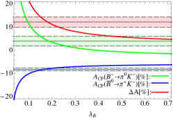
Figure 5: The dependance of the direct $CP$ asymmetries $A_{CP}(B^{-}\to\pi^{0}K^{-})$, $A_{CP}(\bar{B}^{0}\to\pi^{+}K^{-})$ and their difference $\Delta A$ on $\lambda_{B}$ (in unites of GeV) with the fitted annihilation parameters of scenario I (Part A). Their experimental results with $1\sigma$ error are shown by shaded bands with the same color as the lines.

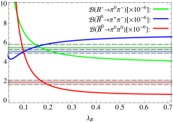
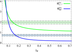
Figure 6: The dependence of the branching fractions ${\cal B}(B^{-}\to\pi^{-}\pi^{0})$, ${\cal B}(\bar{B}^{0}\to\pi^{+}\pi^{-})$, ${\cal B}(\bar{B}^{0}\to\pi^{0}\pi^{0})$ and ratios $R_{+-}^{\pi\pi}$, $R_{00}^{\pi\pi}$ on $\lambda_{B}$ with the same notes as Fig.5.

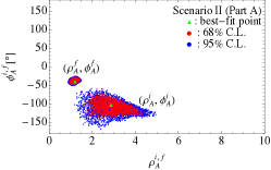
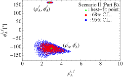
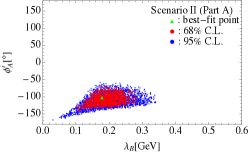
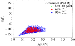
Figure 7: The allowed regions of annihilation parameters ($\rho_{A}^{i,f}$, $\phi_{A}^{i,f}$) and $\lambda_{B}$ at $68\%$ C.L. and $95\%$ C.L.. The best-fit points of part A and B correspond to $\chi^{2}_{\rm min}=3.66$ and $\chi^{2}_{\rm min}=3.67$, respectively.

Table 5: Numerical results of annihilation parameters and moment parameter $\lambda_{B}$ in Scenario II.

	$\rho_{A}^{i}$	$\phi_{A}^{i}[^{\circ}]$	$\rho_{A}^{f}$	$\phi_{A}^{f}[^{\circ}]$	$\lambda_{B}$ [GeV]
Part A	$2.88^{+1.52}_{-1.30}$	$-103^{+33}_{-40}$	$1.21^{+0.22}_{-0.25}$	$-40^{+12}_{-8}$	$0.18^{+0.11}_{-0.08}$
Part B	$2.98^{+1.50}_{-1.40}$	$-106^{+35}_{-39}$	$2.78^{+0.29}_{-0.18}$	$165^{+4}_{-3}$	$0.19^{+0.09}_{-0.10}$

To explicitly show the effects of spectator scattering contributions on $\pi K$ puzzle, dependance of $A_{CP}(B^{-}\to\pi^{0}K^{-})$, $A_{CP}(\bar{B}^{0}\to\pi^{+}K^{-})$ and their difference $\Delta A$ on parameter $\lambda_{B}$ are displayed in Fig.5. It is found that (1) observables of $A_{CP}(B^{-}\to\pi^{0}K^{-})$ and $\Delta A$ are more sensitive to variation of $\lambda_{B}$ than $A_{CP}(\bar{B}^{0}\to\pi^{+}K^{-})$ in the region of $\lambda_{B}$ $\geq$ 100 MeV. The reason is aforementioned fact that coefficient $\alpha_{2}$ in amplitude ${\cal A}_{B^{-}\to\pi^{0}K^{-}}$ [see Eq.(12)] receives significant spectator scattering corrections. A noticeable change of observables is easily seen in the low region of $\lambda_{B}$ because spectator scattering corrections are inversely proportional to $\lambda_{B}$ [see Eq.(10) and Eq.(39)]. (2) a relative small value of $\lambda_{B}$ $\in$ [150 MeV, 220 MeV], as expected in lambda , is required to confront with available measurements. Especially, the value $\lambda_{B}$ $\approx$ 190 MeV provides a perfect description of the experimental data on $A_{CP}(B^{-}\to\pi^{0}K^{-})$, $A_{CP}(\bar{B}^{0}\to\pi^{+}K^{-})$ and $\Delta A$ simultaneously. For $B$ $\to$ $\pi\pi$ decays, from Eqs.(18-20), it is easily seen that amplitude ${\cal A}_{B^{-}\to\pi^{-}\pi^{0}}$ $\propto$ $\alpha_{1}$ + $\alpha_{2}$, ${\cal A}_{\bar{B}^{0}\to\pi^{+}\pi^{-}}$ $\propto$ $\alpha_{1}$, ${\cal A}_{\bar{B}^{0}\to\pi^{0}\pi^{0}}$ $\propto$ $\alpha_{2}$. The coefficient $\alpha_{2}$, corresponding to the color-suppressed tree contribution, its value is small relative to $\alpha_{1}$, so the experimental data on $R_{+-}^{\pi\pi}$ can be well explained with scenario S4 QCDF where $X_{A}^{i}$ $=$ $X_{A}^{f}$ and $\rho_{A}^{f,i}$ = 1 (see Table 2). But as to observable $R_{00}^{\pi\pi}$ or/and branching ratio ${\cal B}(\bar{B}^{0}\to\pi^{0}\pi^{0})$, an enhanced $\alpha_{2}$ is desirable. Hence, the nonfactorizable spectator scattering contributions, which have significant effects on $\alpha_{2}$, would play an important role in studying the color-suppressed tree $B$ decays, and possibly provide a solution to the $\pi\pi$ puzzle. The dependencies of the branching fractions of $B$ $\to$ $\pi\pi$ decays and ratios $R_{+-}^{\pi\pi}$, $R_{00}^{\pi\pi}$ on $\lambda_{B}$ are shown in Fig.6 where the fitted parameters of Part A in Table 1 is used. It is interesting that beside a large value $\rho_{H}$, a small value of $\lambda_{B}$ $\sim$ 200 MeV is also required to confront with experimental data on ${\cal B}(B\to\pi\pi)$, $R_{+-}^{\pi\pi}$ and $R_{00}^{\pi\pi}$.

With the available experimental data on $B$ $\to$ $\pi\pi$, $\pi K$ and $K\bar{K}$ decays, we perform a comprehensive fit on both annihilation parameters ($\rho_{A}^{i,f}$, $\phi_{A}^{i,f}$) and $B$-meson wave function parameter $\lambda_{B}$. The allowed parameter spaces are shown in Fig.7, and the corresponding numerical results are summarized in Table 5. Like scenario I, there are two allowed spaces which are labelled by part A and B. It is easily found that (1) parameters $(\rho_{A}^{i},\phi_{A}^{i})$ $=$ $(\rho_{H},\phi_{H})$ are still required to have large values (see Table 5), that is to say, it is necessary for penguin-dominated or color-suppressed tree $B$ decays to own large corrections from nonfactorizable annihilation and spectator scattering topologies. (2) There is still no overlap between the regions of $(\rho_{A}^{f},\phi_{A}^{f})$ and $(\rho_{A}^{i},\phi_{A}^{i})$ at the 95% confidence level. (3) The cental values of $\rho_{A}^{i,f}$ are a little larger than those in scenario I. The uncertainties on $(\rho_{A}^{i},\phi_{A}^{i})$ are a little smaller than those in scenario I, because more processes from $B$ $\to$ $\pi\pi$ decays are considered in fitting and the amplitudes for $B$ $\to$ $\pi\pi$ decays are sensitive to $X_{A}^{i}$ and $X_{H}$ rather than $X_{A}^{f}$. (4) A small value of parameter $\lambda_{B}$ $\leq$ 350 MeV at the 95% confidence level is strongly required to reconcile discrepancies between results of QCDF approach and available experimental data on $B$ $\to$ $\pi\pi$, $\pi K$ and $K\bar{K}$ decays.

The two solutions of scenario II, Part A and B, will give similar results, as discussed before. With the best fit parameters of Part A in Table 5, we present our evaluations on branching ratios, direct and mixing-induced $CP$ asymmetries for $B_{u,d}$ ${\to}$ $\pi K$, $K\bar{K}$, $\pi\pi$ decays in the “scenario II” column of Table 2, 3 and 4, respectively. It is found that the central values of branching ratios for $B$ $\to$ $\pi\pi$, $\pi K$ and $K\bar{K}$ decays, expect $\bar{B}^{0}$ $\to$ $\pi^{+}\pi^{-}$ decay, with the Part A parameters of scenario II, are a little larger than those of scenario I (see Table 2), because a bit larger values of $\rho_{A}^{i,f}$ and a bit smaller value of $\lambda_{B}$ than those of scenario I are taken in scenario II. Compared with results of scenario S4 QCDF, agreement between theoretical results within two scenarios and experimental measurements is improved, especially for the observables $\Delta A$, $R_{00}^{\pi\pi}$ and $A_{CP}(B^{0}\to\pi\pi)$.

III.3 Scenario III

The above analyses and results are based on the assumption that $X_{A}^{i}$ $=$ $X_{H}$ (i.e. $(\rho_{A}^{i},\phi_{A}^{i})$ $=$ $(\rho_{H},\phi_{H})$) for simplicity. While, there is no compellent requirement for such simplification, except for the fact that wave functions of $B$ mesons are involved in the convolution integrals of both spectator scattering and nonfactorizable annihilation corrections, but are irrelevant to the factorable annihilation amplitudes. So, as a general scenario (named scenario III), we would reevaluate the strength of annihilation and hard-spectator contributions without any simplification for the parameters $(\rho_{A}^{i},\phi_{A}^{i})$, $(\rho_{A}^{i},\phi_{A}^{i})$ and $(\rho_{H},\phi_{H})$.

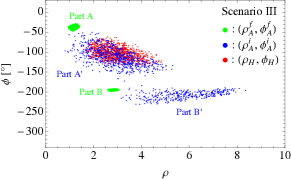
Figure 8: The allowed regions of annihilation and hard-spectator parameters ($\rho_{A}^{f}$, $\phi_{A}^{f}$), ($\rho_{A}^{i}$, $\phi_{A}^{i}$) and ($\rho_{H}$, $\phi_{H}$) at $68\%$ C.L.. The two solutions of ($\rho_{A}^{f}$, $\phi_{A}^{f}$) and ($\rho_{A}^{i}$, $\phi_{A}^{i}$) are labeled as Part A, B and $\rm A^{\prime}$, $\rm B^{\prime}$, respectively.

Considering the constraints from observables of $B_{u,d}$ ${\to}$ $K\bar{K}$, ${\pi}K$ and ${\pi}{\pi}$ decays, a fit for the annihilation and hard-spectator parameters is performed again. In this fit, $(\rho_{A}^{f},\phi_{A}^{f})$, $(\rho_{A}^{i},\phi_{A}^{i})$ and $(\rho_{H},\phi_{H})$ are treated as six free parameters. Moreover, from the hard-spectator corrections illustrated by Eq. (39), it can be seen that $\lambda_{B}$ and $X_{H}$ are always combined together.

Although the inverse moment $\lambda_{B}$ of $B$ wave function could be determined or constricted by further experiments Beneke5 ; BaBarBA1 ; BaBarBA2 ; lambda , $\lambda_{B}$ is more like a free parameter for the moment due to loose limitation on it. So it is impossible to strictly bound on $\lambda_{B}$ and $X_{H}$ simultaneously due to the interference effects between them. In our following fit, we will fix $\lambda_{B}=200\,{\rm MeV}$. Our fitting results at $68\%$ C.L. are presented in Fig. 8, where the range of ${\phi}$ ${\in}$ $[-360^{\circ},0^{\circ}]$ is assigned to illustrate their relative magnitude. Numerically, we get

$$(\rho_{A}^{f},\phi_{A}^{f}[^{\circ}])=\left\{\begin{array}[]{ll}&(1.18^{+0.26}_{-0.23},-40^{+12}_{-8})\qquad\text{Part A }\\ &(2.79^{+0.26}_{-0.20},-196^{+5}_{-3})\qquad\text{Part B }\end{array}\right.$$ (29)

$$(\rho_{A}^{i},\phi_{A}^{i}[^{\circ}])=\left\{\begin{array}[]{ll}&(2.85^{+2.18}_{-1.92},-103^{+52}_{-63})\qquad\text{Part ${\rm A}^{\prime}$ }\\ &(6.54^{+1.81}_{-3.30},-206^{+23}_{-24})\qquad\text{Part ${\rm B}^{\prime}$ }\end{array}\right.$$ (32)

$$(\rho_{H},\phi_{H}[^{\circ}])=(3.09^{+1.64}_{-1.53},-102^{+40}_{-31})\,.$$ (33)

It can be easily seen from Fig. 8 that: (1) for factorizable annihilation parameters $(\rho_{A}^{f},\phi_{A}^{f})$, similar to scenarios I and II, there are two allowed regions (labelled by part A and B); (2) for nonfactorizable annihilation parameters $(\rho_{A}^{i},\phi_{A}^{i})$, besides the solution similar to scenarios I and II (labelled by part ${\rm A}^{\prime}$), another solution (labelled by part ${\rm B}^{\prime}$) with a very large value of $\rho_{A}^{i}$ is gotten. (3) It is very intersting that the allowed space of $(\rho_{H},\phi_{H})$ overlaps almost entirely with the “part ${\rm A}^{\prime}$” allowed space of $(\rho_{A}^{i},\phi_{A}^{i})$. Moreover, their best-fit points $(\rho_{A}^{i},\phi_{A}^{i})$ $=$ $(2.85,-103^{\circ})$ of “part ${\rm A}^{\prime}$” and $(\rho_{H},\phi_{H})$ $=$ $(3.09,-102^{\circ})$ are very close to each other. It might imply that the assumption $X_{A}^{i}$ $(\rho_{A}^{i},\phi_{A}^{i})$ $=$ $X_{H}$ $(\rho_{H},\phi_{H})$ used in scenarios I and II is a good simplification.

With the best fit parameters in scenarios III, either the small value of $\rho_{A}^{i}$ in “part ${\rm A}^{\prime}$” or the large value in “part ${\rm B}^{\prime}$”, our evaluations on branching ratios, direct and mixing-induced $CP$ asymmetries for $B_{u,d}$ ${\to}$ $\pi K$, $K\bar{K}$, $\pi\pi$ decays are similar to those given in our scenarios I and II, so no longer listed here. For the two solutions ${\rm A}^{\prime}$ and ${\rm B}^{\prime}$ of $(\rho_{A}^{i},\phi_{A}^{i})$, it is expected by QCDF approach Beneke2 that the parameter $\rho_{A}^{i}$ should have a small value, which is also favored by our scenarios I and II fit. In fact, such two solutions lead to the same results of $A^{i}_{1,2}$, but the different ones of $A^{i}_{3}$, which principally provides an opportunity to refute one of them. However, because $A^{i}_{3}$ is numerically trivial due to $(r_{\chi}^{M_{1}}-r_{\chi}^{M_{2}})\sim 0$ for the light mesons, such way is practically unfeasible for current accuracies of theoretical calculation and experimentally measurement.

IV Conclusions

The recent CDF and LHCb measurements of large branching ratios for pure annihilation $\bar{B}_{s}^{0}$ $\to$ $\pi^{+}\pi^{-}$ and $\bar{B}_{d}^{0}$ $\to$ $K^{+}K^{-}$ decays imply possible large annihilation contributions, which induce us to modify the traditional QCDF treatment for annihilation parameters. Following the suggestion of Ref.zhu2 , two sets of annihilation parameters $X_{A}^{i}$ and $X_{A}^{f}$ are used to parameterize the endpoint singularity in nonfactorizable and factorizable annihilation amplitudes, respectively. Besides annihilation effects, the resolution of so-called ${\pi}K$ and ${\pi}{\pi}$ puzzles also expect constructive contributions from spectator scattering topologies. With the approximation of $X_{A}^{i}$ $=$ $X_{H}$, we perform a global fit on both annihilation parameters ($\rho_{A}^{i,f}$, $\phi_{A}^{i,f}$) and $B$-meson wave function parameter $\lambda_{B}$ based on available experimental data for $B$ $\to$ $\pi\pi$, $\pi K$ and $K\bar{K}$ decays. Our main conclusions and findings are summarized as:

• The $95\%$ C.L. allowed region of $(\rho_{A}^{i},\phi_{A}^{i})$ is entirely different from that of $(\rho_{A}^{f},\phi_{A}^{f})$. This fact means that the traditional QCDF treatment $(\rho_{A},\phi_{A})$ as universal parameters for different annihilation topologies might be unapplicable to hadronic $B$ decays.

• The current experimental data on $B$ $\to$ $\pi\pi$, $\pi K$ and $K\bar{K}$ decays seems to favor a large value of $\rho_{A}^{i}$ $\sim$ 2.9, which corresponds to a sizable nonfactorizable annihilation contributions. But the range of $(\rho_{A}^{i},\phi_{A}^{i})$ is still very large, because the measurement precision of $CP$ asymmetries is low now.

• There are two possible choices for parameters $(\rho_{A}^{f},\phi_{A}^{f})$. One is $(\rho_{A}^{f},\phi_{A}^{f})$ $\sim$ $(1.1,-40^{\circ})$, the other is $(\rho_{A}^{f},\phi_{A}^{f})$ $\sim$ $(2.7,165^{\circ})$. These two choices correspond to similar factorizable annihilation contributions, although the QCDF approach tends to have a small value of $\rho_{A}^{f}$ Beneke2 . The space for $(\rho_{A}^{f},\phi_{A}^{f})$ is relatively tight due to the well measured branching ratios for $B$ $\to$ $\pi\pi$, $\pi K$ and $K\bar{K}$ decays.

• The spectator scattering corrections play an important role in resolving both $\pi K$ and $\pi\pi$ puzzles. Within QCDF approach, the spectator scattering amplitudes depend on parameters $(\rho_{H},\phi_{H})$ and $B$-meson wave function parameter $\lambda_{B}$. In our analysis, the approximation $(\rho_{H},\phi_{H})$ $=$ $(\rho_{A}^{i},\phi_{A}^{i})$ is assumed, which is proven to be a good simplification by a global fit in scenario III. A small value of $\lambda_{B}$ $\leq$ 350 MeV at the 95% C.L. is obtained by the global fit on $B$ $\to$ $\pi\pi$, $\pi K$ and $K\bar{K}$ decays, which needs to be further tested by future improved measurement on $B$ $\to$ $\ell\nu_{\ell}\gamma$ decays. An enhanced color-suppressed tree coefficient $\alpha_{2}$, which is supported by both large value of $\rho_{H}$ $\sim$ 2.9 and small value of $\lambda_{B}$ $\sim$ 200 MeV, is helpful to reconcile discrepancies on $\Delta A$ and $R_{00}^{\pi\pi}$ between QCDF approach and experiments.

The spectator scattering and annihilation contributions can offer significant corrections to observables of hadronic $B$ decays, and deserve intensive research especially when we apply the QCDF approach to the penguin-dominated, color-suppressed tree, and pure annihilation nonleptonic $B$ decays. As suggested in Ref.zhu1 ; zhu2 and proofed by the pQCD approach pqcd , different parameters corresponding to different topologies should be introduced to regulate the endpoint divergences in spectator scattering and annihilation amplitudes within QCDF approach, even parameters reflecting the flavor symmetry-breaking effects should be considered for $B_{u,d,s}$ decays zhu1 ; zhu2 ; Cheng1 ; Cheng2 ; Cheng3 ; Beneke2 ; chang1 . This treatment might provide possible solution to “problematic” discrepancies between QCDF results and available measurements. Of course, a fine-tuning of these parameters is required to be compatible with the experimental constraints. With the running LHCb and the upcoming SuperKEKB experiments, more refined measurements on $B$-meson decays can be obtained, which will provide more powerful grounds to test various approach and confirm or refute some theoretical hypotheses.

Appendix A Building blocks of annihilation and spectator scattering contributions

The annihilation amplitudes for two-body nonleptonic $B$ $\to$ $M_{1}M_{2}$ decays (here $M_{i}$ denotes the light pseudoscalar meson) can be expressed as the following building blocks Beneke2 ,

$$A_{1}^{i} = \pi\alpha_{s}\int_{0}^{1}dxdy\Big{\{}\Phi_{M_{2}}^{a}(x)\Phi_{M_{1}}^{a}(y)\Big{[}\frac{1}{y(1-x\bar{y})}+\frac{1}{\bar{x}^{2}y}\Big{]}+r_{\chi}^{M_{1}}r_{\chi}^{M_{2}}\frac{2\Phi_{M_{2}}^{p}(x)\Phi_{M_{1}}^{p}(y)}{\bar{x}y}\Big{\}},$$ (34)

$$A_{2}^{i} = \pi\alpha_{s}\int_{0}^{1}dxdy\Big{\{}\Phi_{M_{2}}^{a}(x)\Phi_{M_{1}}^{a}(y)\Big{[}\frac{1}{\bar{x}(1-x\bar{y})}+\frac{1}{\bar{x}y^{2}}\Big{]}+r_{\chi}^{M_{1}}r_{\chi}^{M_{2}}\frac{2\Phi_{M_{2}}^{p}(x)\Phi_{M_{1}}^{p}(y)}{\bar{x}y}\Big{\}},$$ (35)

$$A_{3}^{i} = \pi\alpha_{s}\int_{0}^{1}dxdy\Big{\{}r_{\chi}^{M_{1}}\frac{2\bar{y}\ \Phi_{M_{2}}^{a}(x)\Phi_{M_{1}}^{p}(y)}{\bar{x}y(1-x\bar{y})}-r_{\chi}^{M_{2}}\frac{2x\ \Phi_{M_{1}}^{a}(y)\Phi_{M_{2}}^{p}(x)}{\bar{x}y(1-x\bar{y})}\Big{\}},$$ (36)

$$A_{1}^{f} = A_{2}^{f}=0,$$ (37)

$$A_{3}^{f} = \pi\alpha_{s}\int_{0}^{1}dxdy\Big{\{}r_{\chi}^{M_{1}}\frac{2(1+\bar{x})\ \Phi_{M_{2}}^{a}(x)\Phi_{M_{1}}^{p}(y)}{\bar{x}^{2}y}+r_{\chi}^{M_{2}}\frac{2(1+y)\ \Phi_{M_{1}}^{a}(y)\Phi_{M_{2}}^{p}(x)}{\bar{x}y^{2}}\Big{\}},$$ (38)

where the subscripts $k$ on $A^{i,f}_{k}$ correspond to three possible Dirac current structures, namely, $k$ $=$ $1$, $2$, $3$ for $(V-A)\otimes(V-A)$, $(V-A)\otimes(V+A)$, $-2(S-P)\otimes(S+P)$, respectively. $r_{\chi}^{M}$ $=$ $2m_{M}^{2}/m_{b}(m_{1}+m_{2})$, where $m_{1,2}$ are the current quark mass of the pseudoscalar meson with mass $m_{M}$. $\Phi_{M}^{a}$ and $\Phi_{M}^{p}$ are the twist-2 and twist-3 light-cone distribution amplitudes, respectively. Their asymptotic forms are $\Phi_{M}^{a}(x)$ $=$ $6x\bar{x}$ and $\Phi_{M}^{p}(x)$ $=$ $1$.

The spectator scattering corrections are given by Beneke2

$$H_{i}(M_{1}M_{2})=\left\{\begin{array}[]{l}\displaystyle+\frac{B_{M_{1}M_{2}}}{A_{M_{1}M_{2}}}{\int}_{0}^{1}d{\xi}\frac{\Phi_{B}(\xi)}{\xi}\int_{0}^{1}dxdy\Big{[}\frac{\Phi_{M_{2}}^{a}(x)\Phi_{M_{1}}^{a}(y)}{\bar{x}\bar{y}}+r_{\chi}^{M_{1}}\frac{\Phi_{M_{2}}^{a}(x)\Phi_{M_{1}}^{p}(y)}{x\bar{y}}\Big{]},\\ \qquad\qquad\qquad\text{for }\,i=1,2,3,4,9,10\\ \displaystyle-\frac{B_{M_{1}M_{2}}}{A_{M_{1}M_{2}}}{\int}_{0}^{1}d{\xi}\frac{\Phi_{B}(\xi)}{\xi}\int_{0}^{1}dxdy\Big{[}\frac{\Phi_{M_{2}}^{a}(x)\Phi_{M_{1}}^{a}(y)}{x\bar{y}}+r_{\chi}^{M_{1}}\frac{\Phi_{M_{2}}^{a}(x)\Phi_{M_{1}}^{p}(y)}{\bar{x}\bar{y}}\Big{]},\\ \qquad\qquad\qquad\text{for }\,i=5,7\\ 0,\qquad\qquad\quad\text{for }\,i=6,8\end{array}\right.$$ (39)

where the factorized matrix elements are parameterized as Beneke2

$$A_{M_{1}M_{2}}=i\frac{G_{F}}{\sqrt{2}}m_{B}^{2}F_{0}^{B{\to}M_{1}}f_{M_{2}},\qquad\qquad B_{M_{1}M_{2}}=i\frac{G_{F}}{\sqrt{2}}f_{B}f_{M_{1}}f_{M_{2}}.$$ (40)

Appendix B Theoretical input parameters

For the CKM matrix elements, we adopt the fitting results for the Wolfenstein parameters given by the CKMfitter group CKMfitter

$$\bar{\rho}=0.140^{+0.027}_{-0.026},\quad\bar{\eta}=0.343^{+0.015}_{-0.014},\quad A=0.802^{+0.029}_{-0.011},\quad\lambda=0.22543^{+0.00059}_{-0.00094}.$$ (41)

The pole masses of quarks are PDG12

$$m_{u}=m_{d}=m_{s}=0,\quad m_{c}=1.67\pm 0.07\,{\rm GeV},$$

$$m_{b}=4.78\pm 0.06\,{\rm GeV},\quad m_{t}=173.5\pm 1.0\,{\rm GeV}.$$ (42)

The running masses of quarks are PDG12

$$\frac{\bar{m}_{s}(\mu)}{\bar{m}_{q}(\mu)}=27\pm 1,\quad\bar{m}_{s}(2\,{\rm GeV})=95\pm 5\,{\rm MeV},\quad\bar{m}_{c}(\bar{m}_{c})=1.275\pm 0.025\,{\rm GeV},$$

$$\bar{m}_{b}(\bar{m}_{b})=4.18\pm 0.03\,{\rm GeV},\quad\bar{m}_{t}(\bar{m}_{t})=160.0^{+4.8}_{-4.3}\,{\rm GeV}.$$ (43)

The decay constants of $B$-meson and light mesons are PDG12

$$f_{B}=(0.190\pm 0.013)\,{\rm GeV},\quad f_{\pi}=(130.4\pm 0.2)\,{\rm MeV},\quad f_{K}=(156.1\pm 0.8)\,{\rm MeV}.$$ (44)

We take the following heavy-to-light transition form factors BallZwicky

$$F^{B\to\pi}_{0}(0)=0.258\pm 0.031,\qquad F^{B\to K}_{0}(0)=0.331\pm 0.041.$$ (45)

Moreover, for the Gegenbauer coefficients, we take BallG

$$a_{1}^{\pi}({\rm 2GeV})=0,\quad a_{2}^{\pi}({\rm 2GeV})=0.17,\quad a_{1}^{K}({\rm 2GeV})=0.05,\quad a_{2}^{K}({\rm 2GeV})=0.17.$$ (46)

For the other inputs, such as the masses and lifetimes of mesons and so on, we take their central values given by PDG PDG12 .

Appendix C Fitting Approach

Our fit is performed in a simple way, which is similar to the one adopted in Ref.Vernazza based on the frequentist framework. Considering a set of $N$ observables $f_{j}$, the experimental measurements are assumed to be Gaussian distributed with the mean value $f_{j\,\rm exp}$ and error $\sigma_{j\,\rm exp}$. The theoretical prediction $f_{j\,\rm theo}$ for each observable could be treated as a function of a set of “unknown” free parameters $\{y_{i}\}$ (here $y_{i}$ $=$ $\rho_{A}^{i,f}$, $\phi_{A}^{i,f}$ and $\lambda_{B}$ in this paper). To estimate the values of “unknown” parameters $\{y_{i}\}$ and compare the theoretical results $f_{j\,\rm theo}$ with the experimental data $f_{j\,\rm exp}$, typically, it is need to construct a $\chi^{2}$ function as

$$\chi^{2}(\{y_{i}\})=\sum\limits_{j=1}^{N}\frac{(f_{j\,\rm theo}(\{y_{i}\})-f_{j\,\rm exp})^{2}}{\sigma_{j\,\rm exp}^{2}}.$$ (47)

In the evaluation of $f_{j\,\rm theo}$ for hadronic B decays, ones always encounter theoretical uncertainties induced by input parameters, like form factor and decay constant, whose probability distribution is unknown. Following the treatment of Rfit scheme CKMfitter ; Rfit that input values are treated on an equal footing, irrespective of how close they are from the edge of the allowed range, the $\chi^{2}$ function is modified as Vernazza

$$\chi^{2}=\sum_{j=1}^{N}\left\{\begin{array}[]{cl}\displaystyle\frac{([f_{j\,\rm theo}-\delta_{j\,\rm theo,\,sub}]-f_{j\,\rm exp})^{2}}{\sigma_{j\,\rm exp}^{2}}&\quad\text{if }f_{j\,\rm exp}<[f_{j\,\rm theo}-\delta_{j\,\rm theo,\,sub}],\\ \displaystyle\frac{(f_{j\,\rm exp}-[f_{j\,\rm theo}+\delta_{j\,\rm theo,\,sup}])^{2}}{\sigma_{j\,\rm exp}^{2}}&\quad\text{if }f_{j\,\rm exp}>[f_{j\,\rm theo}+\delta_{j\,\rm theo,\,sup}],\\ 0&\quad\text{otherwise}\end{array}\right.$$ (48)

where $\delta_{j\,\rm theo,\,sup}$ and $\delta_{j\,\rm theo,\,sub}$ denote asymmetric theoretical uncertainties, and are defined as $(f_{j\,\rm theo})^{+\delta_{j\,\rm theo,\,sup}}_{-\delta_{j\,\rm theo,\,sub}}$. As to the asymmetric experimental errors, we choose the larger one as weighting factor. Correspondingly, the confidence levels are defined by the function

$${\rm CL}(\{y_{i}\})=\frac{1}{\sqrt{2^{N_{\rm dof}}}\Gamma(N_{\rm dof}/2)}\int_{\Delta\chi^{2}(\{y_{i}\})}^{\infty}e^{-t/2}t^{N_{\rm dof}/2-1}dt,$$ (49)

with $\Delta\chi^{2}$ $=$ $\chi^{2}$ $-$ $\chi^{2}_{\rm min}$ and $N_{\rm dof}$ the number of degrees of freedom of free parameters.

With the input parameters summarized in Appendix B, we scan the space of the parameters $y_{i}$ and calculate the theoretical results $f_{j\,\rm theo}$. The $\chi^{2}$ could be obtained with Eq.(48). The numerical results at $1\sigma$ and $2\sigma$ confidence levels are gotten from Eq.(49) by taking ${\rm CL}$ $=$ $1-68.27\%$ and ${\rm CL}$ $=$ $1-95.45\%$, respectively.

References

- (1) T. Aaltonen et al. (CDF Collaboration), Phys. Rev. Lett. 108 (2012) 211803 [arXiv:1111.0485].
- (2) R. Aaij et al. (LHCb Collaboration), JHEP 1210 (2012) 037 [arXiv:1206.2794].
- (3) Y. Amhis et al. (HFAG), arXiv:1207.1158; and online update at: http://www.slac.stanford.edu/xorg/hfag.
- (4) G. H. Zhu, Phys. Lett. B 702 (2011) 408 [arXiv:1106.4709].
- (5) K. Wang and G. H. Zhu, Phys. Rev. D 88 (2013) 014043 [arXiv:1304.7438].
- (6) Q. Chang, X. W. Cui, L. Han and Y. D. Yang, Phys. Rev. D 86 (2012) 054016 [arXiv:1205.4325].
- (7) Z. J. Xiao, W. F. Wang and Y. Y. Fan, Phys. Rev. D 85 (2012) 094003 [arXiv:1111.6264].
- (8) Y. Y. Keum, H. N. Li and A.I. Sanda, Phys. Lett. B 504 (2001) 6 [arXiv:hep-ph/0004004]; Y. Y. Keum, H. N. Li and A.I. Sanda, Phys. Rev. D 63 (2001) 054008 [arXiv:hep-ph/0004173]; C. D. Lu, K. Ukai and M.-Z. Yang, Phys. Rev. D 63 (2001) 074009 [arXiv:hep-ph/0004213].
- (9) A. Ali, G. Kramer, Y. Li, C. D. Lu, Y. L. Shen, W. Wang and Y. M. Wang, Phys. Rev. D 76 (2007) 074018 [arXiv:hep-ph/0703162]; Y. Li and C. D. Lu, Commun. Theor. Phys. 44 (2005) 659 [arXiv:hep-ph/0502038].
- (10) D. Du, H, Gong, J. Sun, D. Yang, and G. Zhu, Phys. Rev. D 65 (2002) 074001 [arXiv:hep-ph/0108141]; Phys. Rev. D 65 (2002) 094025 Erratum, ibid. 66 (2002) 079904 [arXiv:hep-ph/0201253]; J. Sun, G. Zhu and D. Du, Phys. Rev. D 68 (2003) 054003 [arXiv:hep-ph/0211154].
- (11) M. Beneke, G. Buchalla, M. Neubert and C. T. Sachrajda, Nucl. Phys. B 606 (2001) 245 [arXiv:hep-ph/0104110]; M. Beneke and M. Neubert, Nucl. Phys. B 651 (2003) 225 [arXiv:hep-ph/0210085]; M. Beneke and M. Neubert, Nucl. Phys. B 675 (2003) 333 [arXiv:hep-ph/0308039].
- (12) M. Beneke, G. Buchalla, M. Neubert and C. T. Sachrajda, Phys. Rev. Lett. 83 (1999) 1914 [arXiv:hep-ph/9905312]; Nucl. Phys. B 591 (2000) 313 [arXiv:hep-ph/0006142].
- (13) H. Y. Cheng and C. K. Chua, Phys. Rev. D 80 (2009) 114026 [arXiv:0910.5237].
- (14) H. Y. Cheng and C. K. Chua, Phys. Rev. D 80 (2009) 114008 [arXiv:0909.5229].
- (15) A. J. Buras, R. Fleischer, S. Recksiegel and F. Schwab, Phys. Rev. Lett. 92 (2004) 101804 [arXiv:hep-ph/0312259]; Nucl. Phys. B 697 (2004) 133 [arXiv:hep-ph/0402112].
- (16) G. Buchalla, A. J. Buras, and M. E. Lautenbacher, Rev. Mod. Phys. 68 (1996) 1125 [arXiv:hep-ph/9512380]; A. J. Buras, arXiv:hep-ph/9806471; arXiv:hep-ph/0101336.
- (17) H. Y. Cheng and C. K. Chua, Phys. Rev. D 80 (2009) 074031 [arXiv:0908.3506].
- (18) M. Beneke and J. Rohrwild, Eur. Phys. J. C 71 (2011) 1818 [arXiv:1110.3228].
- (19) M. Beneke, J. Rohrer and D. S. Yang, Nucl. Phys. B 774 (2007) 64 [arXiv:hep-ph/0612290].
- (20) V. M. Braun, D.Yu. Ivanov, G. P. Korchemsky, Phys. Rev. D 69 (2004) 034014 [arXiv:hep-ph/0309330].
- (21) B. Aubert et al. (BaBar Collaboration), arXiv:0704.1478.
- (22) B. Aubert et al. (BaBar Collaboration), Phys. Rev. D 80 (2009) 111105 [arXiv:0907.1681].
- (23) M. Beneke, S. Jäger, Nucl. Phys. B 751 (2006) 160 [arXiv:hep-ph/0512351]; G. Bell, V. Pilipp, Phys. Rev. D 80 (2009) 054024 [arXiv:0907.1016]; M. Beneke, T. Huber, X. Q. Li, Nucl. Phys. B 832 (2010) 109 [arXiv:0911.3655].
- (24) J. Charles et al. (CKMfitter Group), Eur. Phys. J. C 41, 1 (2005); updated results and plots available at: http://ckmfitter.in2p3.fr.
- (25) J. Beringer et al. (Particle Data Group), Phys. Rev. D 86 (2012) 010001.
- (26) P. Ball and R. Zwicky, Phys. Rev. D 71 (2005) 014015 [arXiv:hep-ph/0406232].
- (27) P. Ball, V. M. Braun, A. Lenz, JHEP 0605 (2006) 004 [arXiv:hep-ph/0603063].
- (28) L. Hofer, D. Scherer and L. Vernazza, JHEP 1102 (2011) 080 [arXiv:1011.6319].
- (29) A. Hocker, H. Lacker, S. Laplace and F. Le Diberder, Eur. Phys. J. C 21 (2001) 225 [arXiv:hep-ph/0104062].