Relativistic entanglement of two particles driven by continuous product momenta

Abstract

In this paper we explore the entanglement of two relativistic spin-$1/2$ particles with continuous momenta. The spin state is described by the Bell state and the momenta are given by Gaussian distributions of product form. Transformations of the spins are systematically investigated in different boost scenarios by calculating the orbits and concurrence of the spin degree of freedom. By visualizing the behavior of the spin state we get further insight into how and why the entanglement changes in different boost situations.

I Introduction

Entanglement is the key notion that distinguishes between the quantum and classical world. It has also proven extremely useful for applications in the context of quantum information theory. While most of the theory of entanglement is non-relativistic, the ultimate description of reality is given by the relativistic theory, thus a complete account of entanglement demands that we understand how entanglement behaves in relativity.

The field of relativistic quantum information, where the first studies appeared a little more than a decade ago, is an attempt to provide such an account Czachor (1997); Gingrich and Adami (2002); Peres et al. (2002); Alsing and Milburn (2002); Ahn et al. (2002, 2003a, 2003b); Czachor and Wilczewski (2003); Moon et al. (2004); Lee and Chang-Young (2004); Czachor (2005); Lamata et al. (2006); Alsing et al. (2006); Chakrabarti (2009); Fuentes et al. (2010); Friis et al. (2010); Palge and Dunningham (2012). The overall conclusion emerging from this work is that relativistic entanglement in both inertial and accelerated frames is observer dependent Alsing and Fuentes (2012). The issue has been in the spotlight since early on. It was found in Gingrich and Adami (2002) that the entanglement of a Bell state generally decreases under Lorentz boosts. Almost simultaneously, it was reported in Alsing and Milburn (2002) that although boosted particles undergo Wigner rotations, the entanglement fidelity of a Bell state remains invariant. This resulted in a number of followup papers, see e.g. Terashima and Ueda (2003); Caban and Rembieliński (2005, 2006); Jordan et al. (2006, 2007), some of which confirm the invariance of entanglement while others claim that entanglement depends on the boost in question. On closer inspection one notices that the (sometimes seemingly contradictory) results in the literature rely on different momentum states and boost angles, or geometries, involved. That geometry plays an instrumental role in determining the behavior of entanglement under Lorentz boosts is also suggested by a study of the simplest system, the single particle Palge and Dunningham (2012). Likewise the literature on the Wigner rotation is quite clear about the fact that its nature is highly geometric, yet barring a few cases Palge et al. (2011), there is almost no work in relativistic quantum information that systematically takes this into account.

In this paper, we aim to fill the lacuna by exploring a number of boost situations with different momenta as well as geometries. The focus is on massive two particle spin-$1/2$ systems whose momentum states are given by continuous distributions of product form . We assume that the spin degree of freedom is described by a maximally entangled Bell state. We visualize the spin state in a 3D manner in order to gain a better understanding of how and why entanglement changes under boosts. The aim of the paper is to provide a simple model that helps explain the various results obtained so far for systems with continuous momenta. Another is to contribute to a survey of different momentum states and geometries in order to have a better view of the landscape of systems that might be of interest for relativistic quantum information theory.

The paper is organized as follows. We begin by outlining how a generic two particle state transforms under Lorentz boosts. The properties of Wigner rotation will then be reviewed, followed by a specification of the models we will study below. Sections VII and VIII give a detailed characterization of the momentum and spin states of the models, respectively. The second half of the paper from section X onwards examines how spin entanglement changes in two particle systems that contain various forms of product momenta. We summarize the results in section XIV.

II General setting

In this paper, we will study a system consisting of two massive spin-$1/2$ particles and ask how the entanglement of spins changes when viewed from a different inertial frame. This question is uninteresting in the non-relativistic setting because boosts do not change the spin state. However, in the relativistic world the situation is non-trivial. The spin seen by an observer in any other frame generally depends on the momentum of the particle and the state of the observer. This entails that spin entanglement in general changes non-trivially too. We begin the discussion by fixing the state space and calculating the generic transformation of a two particle state under Lorentz transformations.

Free spin-$1/2$ particles can be described in two different theories, the unitary irreducible representation of the Poincaré group or in the Dirac theory of bispinors . Throughout we will work in the Wigner representation (also called the Wigner-Bargmann or the spin basis Caban et al. (2013)) and use basis vectors of the form $\mathop{\left|\mathbf{p},\lambda\right\rangle}\equiv\mathop{\left|\mathbf{p}\right\rangle}\mathop{\left|\lambda\right\rangle}\equiv\mathop{\left|\mathbf{p}\right\rangle}\otimes\mathop{\left|\lambda\right\rangle}$, where $\mathbf{p}$ labels the single particle momentum and $\lambda=\pm\frac{1}{2}$ is the spin (see Appendix A for constructions used in the paper). A generic pure two particle state $\mathop{\left|\Psi\right\rangle}\in\mathcal{H}\otimes\mathcal{H}$ can be written as follows,

$$\mathop{\left|\Psi\right\rangle}=\sum_{\lambda\eta}\int\mathrm{d}\mu(p,q)\,\psi_{\lambda\eta}(\mathbf{p},\mathbf{q})\mathop{\left|\mathbf{p},\lambda\right\rangle}\mathop{\left|\mathbf{q},\eta\right\rangle},$$ (1)

where $\mathrm{d}\mu(p)=\left[2E(\mathbf{p})\right]^{-1}\mathrm{d}\mathbf{p}$ is the Lorentz invariant integration measure, we have abbreviated $\mathrm{d}\mu(p,q)=\mathrm{d}\mu(p)\mathrm{d}\mu(q)$ and $\mathcal{H}=L^{2}(\mathbb{R}^{3})\otimes\mathbb{C}^{2}$ denotes the single particle states space. The wave function satisfies the normalization condition

$$\sum_{\lambda\eta}\int\,\mathrm{d}\mu(p,q)|\psi_{\lambda\eta}(\mathbf{p},\mathbf{q})|^{2}=1,$$ (2)

and the (improper) spin and momentum eigenstates satisfy the orthogonality condition

$$\langle\mathbf{p}^{\prime},\lambda^{\prime}|\mathbf{p},\lambda\rangle=2E(\mathbf{p})\delta^{3}(\mathbf{p}-\mathbf{p}^{\prime})\delta_{\lambda\lambda^{\prime}}.$$ (3)

An observer $O^{\Lambda}$ who is Lorentz boosted relative to $O$ by $\Lambda$ describes the same system using a different wave function

$$\psi^{\Lambda}_{\kappa\nu}(\mathbf{p},\mathbf{q}) =\sum_{\lambda\eta}D_{\kappa\lambda}\left[W(\Lambda,\Lambda^{-1}\mathbf{p})\right]D_{\nu\eta}\left[W(\Lambda,\Lambda^{-1}\mathbf{q})\right]$$

$$\phantom{\sum}\times\psi_{\lambda\eta}(\Lambda^{-1}\mathbf{p},\Lambda^{-1}\mathbf{q}),$$ (4)

where $D\left[W(\Lambda,\mathbf{p})\right]\in\mathrm{SU}(2)$ is the spin-$1/2$ representation of the Wigner, or Thomas–Wigner rotation (TWR), $W=L^{-1}(\Lambda L_{p})\Lambda L_{p}$ . This entails that for $O^{\Lambda}$ the spins are rotated by $D[W(\Lambda,\mathbf{p})]$ and the rotation depends on the geometry, i.e. the angle between two boosts as well as the the momenta of the system and the observer. Note that since each spin undergoes a momentum dependent rotation, the result is a non-trivial transformation on the spin degree of freedom of the total two particle state. This implies that properties like entanglement which are defined in terms of spin will change in general as well.

From the logical point of view, we can think of the two particle system as made up of two spin qubits, where each spin qubit is controlled by a momentum system Peres et al. (2002); Gingrich and Adami (2002). The analogy is from quantum information theory where a controlled unitary gate consists of two input qubits which are called the control qubit and the target qubit. The action of the gate is to transform the target qubit with a unitary transformation $U$ depending on the control qubit. One can conceive of the Lorentz boost along the same lines . If momentum takes the role of a control system, then given that the boost angle and rapidity are fixed, the transform on the spin state depends only on the momentum state. While the idea will not enter calculations, the notion of Lorentz boosts as controlled unitaries will guide our investigation of the relativistic spin–momentum systems in this paper. It prompts us to ask the question of what are the maps that different momentum states generate on the spin degree of freedom? This is a broad question and we will not try address it in a single paper. We will approach the topic step-by-step by exploring how a particular subset of interesting momenta drives the spin entanglement. In this paper, we will focus on momenta that are of product form and ask what kind of transformations they induce on the maximally entangled spin state of a two particle system ? Further, while previous work has investigated systems with discrete momenta Palge and Dunningham (2015), which represent idealized models, realistic situations are described by states whose momenta are given by continuous distributions. To understand how the behavior of entanglement is affected when the idealization is dropped we will assume that momenta are given by entangled states that consist of combinations of Gaussians.

III Spin observable

In contrast to the non-relativistic theory, treatment of spin in relativity requires some care. This is due to the fact that the commutation relation of two generators of rotationless Lorentz boosts results in a rotation generator, $[K_{i},N_{j}]=-i\epsilon_{ijk}J_{k}$. The latter is the infinitesimal algebraic form of the TWR. It means that two non-collinear rotationless Lorentz boosts will generate a rotation. From the geometric point of view it is interesting to note that the same phenomenon is related to the fact that the relativistic momentum space, the mass shell hyperbola, is a curved space: a Riemannian space with constant negative curvature Sexl and Urbantke (2001).

While there is some controversy about what is the most adequate spin operator in the relativistic quantum theory, one candidate stands out. It is the so-called Newton-Wigner spin observable, which has advantages over other spins because it possesses a number of properties one naturally demands of a good spin operator. We will give a brief summary of the reasoning that leads to the Newton-Wigner spin. A good overview along with the discussion of the various spin candidates can be found in Caban et al. (2013).

Relativistic quantum theory conceptualizes particles as group representations. Elementary particles correspond to the unitary irreducible representations of the Poincaré group, which are characterized by two labels, mass $m$ and spin $s$. Mass is given by the square root of the eigenvalues of the first Casimir invariant, the mass square operator $P^{2}=P_{\mu}P^{\mu}$. Spin is related to the eigevalues of the second Casimir invariant, $W^{2}=W_{\mu}W^{\mu}$, where

$$W^{\mu}=\frac{1}{2}\epsilon^{\nu\alpha\beta\mu}P_{\nu}J_{\alpha\beta}$$ (5)

is the Pauli-Lubanski vector and $J_{\alpha\beta}$ are the generators of the Lorentz group. The components of $W=(W^{0},W^{j})$ are given by

$$W^{0} =P^{j}M^{j}=\mathbf{P}\cdot\mathbf{M},$$

$$W^{j} =P^{0}M^{j}-\epsilon^{jkl}P^{k}N^{l}=P^{0}M^{j}-(\mathbf{P}\times\mathbf{N})^{j}.$$ (6)

One can then define the spin square operator as

$$\mathbf{S}^{2}=-\frac{1}{m^{2}}W_{\mu}W^{\mu}.$$ (7)

This leads to the idea that the spin operator can be postulated as a linear combination of the components of $W$ given that certain conditions are satisifed, conditions that one would reasonably require of a spin observable. These are as follows, (i) the spin operator $\mathbf{S}$ should fulfill the usual commutation relations,

$$[S^{i},S^{j}]=\mathrm{i}\epsilon_{ijk}S^{k},$$ (8)

(ii) it is a three dimensional vector, that is

$$[J^{i},S^{j}]=\mathrm{i}\epsilon_{ijk}S^{k},$$ (9)

and (iii) in any frame the vector $\mathbf{S}$ is a linear combination of components of $W$ with coefficients that depend only on the four momentum $P^{\mu}$. It can be shown that there is a unique linear combination of operators $W^{\mu}$ which satisfies these conditions and it has the form Bogolubov et al. (1975),

$$\mathbf{S}_{\mathrm{NW}}=\frac{1}{m}\left(\mathbf{W}-\frac{W_{0}}{m+P^{0}}\mathbf{P}\right).$$ (10)

The Newton-Wigner observable corresponds to the Pauli-Lubanski vector which is boosted to the rest frame of the particle MacFarlane (1963),

$$\left(\mathbf{S}_{\mathrm{NW}}\right)^{j}=\frac{1}{m}\left(L^{-1}_{p}W\right)^{j},$$ (11)

where $L^{-1}_{p}$ is the boost that takes momentum $p$ to the rest system of the particle, $L^{-1}_{p}p=(m,0,0,0)$. We will use the Newton-Wigner spin observable $\mathbf{S}_{\mathrm{NW}}$ throughout the paper to characterize the spin of the particles.

Since we are working in the Wigner representation, we need to express $\mathbf{S}_{\mathrm{NW}}$ in that representation. The canonical form of the infinitesimal generators $P^{\mu}$, $\mathbf{M}$ and $\mathbf{N}$ is as follows MacFarlane (1963),

$$P^{\mu} =p^{\mu},$$

$$\mathbf{M} =-i\mathbf{p}\times\partial_{\mathbf{p}}+\mathbf{S},$$ (12)

$$\mathbf{N} =-ip^{0}\partial_{\mathbf{p}}-\frac{\mathbf{p}\times\mathbf{S}}{m+p^{0}},$$

where $\mathbf{S}=\tfrac{1}{2}\bm{\sigma}$ and $\bm{\sigma}=(\sigma_{x},\sigma_{y},\sigma_{z})$ are the Pauli matrices. Substituting the generators (12) into (6) and (10), we obtain for the Newton-Wigner observable

$$\mathbf{S}_{\mathrm{NW}}=\frac{1}{2}\bm{\sigma},$$ (13)

meaning that in the Wigner representation $\mathbf{S}_{\mathrm{NW}}$ is given by the standard Pauli matrices.

IV Spin entanglement

To find how the entanglement of the spin degree of freedom changes in various boost scenarios, we will calculate the boosted spin state $\rho^{\Lambda}_{S}$. The two particle spin state can be written in the operator basis

$$\rho_{S}^{\Lambda}=\frac{1}{4}\left(\mathbb{1}\otimes\mathbb{1}+\mathbf{r}\bm{\sigma}\otimes\mathbb{1}+\mathbb{1}\otimes\mathbf{s}\bm{\sigma}+\sum_{i,j}t_{ij}\sigma_{i}\otimes\sigma_{j}\right),$$ (14)

where the coefficients $\mathbf{r}=(r_{x},r_{y},r_{z})$, $\mathbf{s}=(s_{x},s_{y},s_{z})$ and $t_{ij}$, $i,j\in\{x,y,z\}$ are the expectation values of the spin observables $\bm{\sigma}\otimes\mathbb{1}$, $\mathbb{1}\otimes\bm{\sigma}$ and $\sigma_{i}\otimes\sigma_{j}$. Since the total state of two particles includes momentum as well, i.e. it lives in the space

$$\mathcal{H}^{1}_{p}\otimes\mathcal{H}^{1}_{\lambda}\otimes\mathcal{H}^{2}_{p}\otimes\mathcal{H}^{2}_{\lambda},$$ (15)

the expectation values of observables have the form

$$\langle\mathbf{r}\rangle=\text{Tr}\left(\rho^{\Lambda}\,\mathbb{1}_{p}^{1}\otimes\mathbf{S}_{\mathrm{NW}}^{1}\otimes\mathbb{1}_{p}^{2}\otimes\mathbb{1}_{\sigma}^{2}\right),$$

$$\langle\mathbf{s}\rangle=\text{Tr}\left(\rho^{\Lambda}\,\mathbb{1}_{p}^{1}\otimes\mathbb{1}^{1}_{\sigma}\otimes\mathbb{1}_{p}^{2}\otimes\mathbf{S}_{\mathrm{NW}}^{2}\right),$$ (16)

$$\langle t_{ij}\rangle=\text{Tr}\left(\rho^{\Lambda}\,\mathbb{1}_{p}^{1}\otimes\mathbf{S}_{\mathrm{NW}}^{1}\otimes\mathbb{1}_{p}^{2}\otimes\mathbf{S}_{\mathrm{NW}}^{2}\right),$$

where the superscripts denote the first and the second particle, respectively, and $\rho^{\Lambda}=\mathopen{}\left|{\Psi^{\Lambda}}\right\rangle\!\left\langle{\Psi^{\Lambda}}\right|$.

Entanglement will be quantified by using the concurrence $C(\rho)$. This is necessary since the final spin state $\rho^{\Lambda}$ is generally mixed. Concurrence of a bipartite state $\rho$ of two qubits is defined as

$$C(\rho)=\mathrm{max}\{0,\lambda_{1}-\lambda_{2}-\lambda_{3}-\lambda_{4}\},$$ (17)

where the $\lambda_{i}$ are square roots of eigenvalues of a non-Hermitian matrix $\rho\widetilde{\rho}$ in decreasing order and

$$\widetilde{\rho}=\left(\sigma_{y}\otimes\sigma_{y}\right)\rho^{*}\left(\sigma_{y}\otimes\sigma_{y}\right),$$ (18)

with $\sigma_{y}$ a Pauli matrix, is the spin-flipped state with the complex conjugate ^∗ taken in the standard basis Wootters (1998).

V Thomas–Wigner rotation

The TWR arises from the fact that the subset of Lorentz boosts does not form a subgroup of the Lorentz group. Consider three inertial observers $O$, $O^{\prime}$ and $O^{\prime\prime}$ where $O^{\prime}$ has velocity $\mathbf{v}_{1}$ relative to $O$ and $O^{\prime\prime}$ has $\mathbf{v}_{2}$ relative to $O^{\prime}$. Then the combination of two canonical boosts $\Lambda(\mathbf{v}_{1})$ and $\Lambda(\mathbf{v}_{2})$ that relates $O$ to $O^{\prime\prime}$ is in general a boost and a rotation,

$$\Lambda(\mathbf{v}_{2})\Lambda(\mathbf{v}_{1})=R(\omega)\Lambda(\mathbf{v}_{3}),$$ (19)

where $R(\omega)$ is the TWR with angle $\omega$. To an observer $O$, the frame of $O^{\prime\prime}$ appears to be rotated by $\omega$. We will immediately specialize to massive systems, then $R(\omega)\in\mathrm{SO(3)}$ and $\omega$ is given by (Rhodes and Semon, 2004; Halpern, 1968),

$$\tan\frac{\omega}{2}=\frac{\sin\theta}{\cos\theta+D},$$ (20)

where $\theta$ is the angle between two boosts or, equivalently, $\mathbf{v}_{1}$ and $\mathbf{v}_{2}$, and

$$D=\sqrt{\left(\frac{\gamma_{1}+1}{\gamma_{1}-1}\right)\left(\frac{\gamma_{2}+1}{\gamma_{2}-1}\right)},$$ (21)

with $\gamma_{1,2}=(1-v_{1,2}^{2})^{-1/2}$ and $v_{1,2}=|\mathbf{v}_{1,2}|$. We assume natural units throughout, $\hbar=c=1$. The axis of rotation specified by $\mathbf{n}=\mathbf{v}_{2}\times\mathbf{v}_{1}/|\mathbf{v}_{2}\times\mathbf{v}_{1}|$ is orthogonal to the plane defined by $\mathbf{v}_{1}$ and $\mathbf{v}_{2}$. Using rapidity $\xi_{1,2}=\mathrm{arctanh}\,\left|\mathbf{v}_{1,2}\right|$ to represent the magnitude of the boost and subsuming both under a single parameter $\xi=\xi_{1}=\xi_{2}$, we show the dependence of the TWR on the boost angle $\theta$ and $\xi$ in Fig. 1.

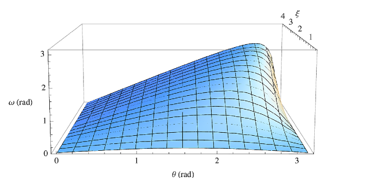
Figure 1: (Color online.) TWR $\omega$ as a function of rapidity $\xi$ and boost angle $\theta$.

Two interesting characteristics are immediately noticeable. First, for any two boosts at a fixed angle $\theta$, the TWR angle $\omega$ increases with $\xi$, approaching a maximum value as boosts approach the speed of light. Second, the angle $\theta$ at which the maximum TWR occurs depends on the magnitude of $\xi$. It is worth noting that $\omega$ approaches the maximum value $180^{\circ}$ when boosts are almost opposite and approach the speed of light. At lower boost magnitudes, maximum rotation occurs earlier.

VI The model

In this section, we will give a broad characterization of the models to be studied below. More detailed discussion of the momentum and spin states will be given in the next two sections.

We will assume throughout that initially the spin and momentum degrees of freedom factorize,

$$\mathop{\left|\Psi\right\rangle}=\int\,\mathrm{d}\mu(p,q)\psi(\mathbf{p},\mathbf{q})\mathop{\left|\mathbf{p},\mathbf{q}\right\rangle}\otimes\mathop{\left|S\right\rangle},$$ (22)

where $\mathop{\left|S\right\rangle}$ is the spin state and momenta are taken to be combinations of Gaussian wave packets in product forms. We start by considering product momenta of the simplest form

$$f_{\mathrm{PQ}}(\mathbf{p},\mathbf{q},\mathbf{p}_{0},\mathbf{q}_{0})=\left[N(\sigma)\right]^{-\frac{1}{2}}g\!\left(\mathbf{p},\mathbf{p}_{0}\right)g\!\left(\mathbf{q},\mathbf{q}_{0}\right),$$ (23)

where $N(\sigma)$ is the normalization and $g(\mathbf{p},\mathbf{p}_{0})$ a Gaussian of width $\sigma$ centered at $\mathbf{p}_{0}=(p_{x0},p_{y0},p_{z0})$,

$$g(\mathbf{p},\mathbf{p}_{0}) =\left[\exp\left(-\frac{\left(p_{x}-p_{x0}\right)^{2}}{2\sigma^{2}}\right)\exp\left(-\frac{\left(p_{y}-p_{y0}\right)^{2}}{2\sigma^{2}}\right)\right.$$

$$\phantom{AA}\left.\times\exp\left(-\frac{\left(p_{z}-p_{z0}\right)^{2}}{2\sigma^{2}}\right)\right]^{\frac{1}{2}}.$$ (24)

There are two slightly different implementations of $f_{\mathrm{PQ}}$ that have been discussed on a number of occasions. When $\mathbf{q}_{0}=-\mathbf{p}_{0}$ we get the familiar EPR–Bohm situation Einstein et al. (1935); Bohm (1951) with two particles moving in opposite directions,

$$f_{\mathrm{EPRB}}(\mathbf{p},\mathbf{q},\mathbf{p}_{0},\mathbf{q}_{0})=f_{\mathrm{PQ}}(\mathbf{p},\mathbf{q},\mathbf{p}_{0},-\mathbf{p}_{0}).$$ (25)

The other realization is described by

$$f_{C}(\mathbf{p},\mathbf{q},\mathbf{p}_{0},\mathbf{q}_{0})=f_{\mathrm{PQ}}(\mathbf{p},\mathbf{q},\mathbf{p}_{Z0},\mathbf{q}_{Z0}),$$ (26)

which we will call axis centered momenta to signify that the centers $\mathbf{p}_{Z0}$, $\mathbf{q}_{Z0}$ of Gaussians lie on a coordinate axis. With no restriction of generality we take the coordinate axis to be the $z$-axis.

Further forms are motivated by observations we made at studying a single particle system, namely, that superposed momenta give rise to maximal entanglement between spin and momentum degrees of freedom. This suggests similar momenta for two particles may give rise to interesting spin–spin effects as well. We will consider a case involving two terms per particle,

$$f_{\Sigma}(\mathbf{p},\mathbf{q},\mathbf{p}_{0},\mathbf{q}_{0}) =\left[N(\sigma)\right]^{-\frac{1}{2}}\left[g\!\left(\mathbf{p},\mathbf{p}_{0}\right)+g\!\left(\mathbf{p},-\mathbf{p}_{0}\right)\right]$$

$$\phantom{A}\times\left[g\!\left(\mathbf{q},\mathbf{q}_{0}\right)+g\!\left(\mathbf{q},-\mathbf{q}_{0}\right)\right]$$ (27)

and a more elaborate one with four terms,

$$f_{\times}(\mathbf{p},\mathbf{q},\mathbf{p}_{0},\mathbf{q}_{0}) =\left[N(\sigma)\right]^{-\frac{1}{2}}\left[g(\mathbf{p},\mathbf{p}_{0})+g(\mathbf{p},-\mathbf{p}_{0})\right.$$

$$\phantom{A}\left.+g(\mathbf{p},\mathbf{p}^{\perp}_{0})+g(\mathbf{p},-\mathbf{p}^{\perp}_{0})\right]\left[g(\mathbf{q},\mathbf{q}_{0})\right.$$

$$\phantom{A}\left.+g(\mathbf{q},-\mathbf{q}_{0})+g(\mathbf{q},\mathbf{q}^{\perp}_{0})+g(\mathbf{q},-\mathbf{q}^{\perp}_{0})\right],$$ (28)

where $\mathbf{p}^{\perp}_{0}$ is a momentum vector of the same magnitude but orthogonal direction to $\mathbf{p}_{0}$ and similarly for $\mathbf{q}^{\perp}_{0}$ and $\mathbf{q}_{0}$.

Boosts are always assumed to be in the $z$-direction, $\Lambda\equiv\Lambda_{z}(\xi)$,

$$\Lambda=\begin{pmatrix}\cosh\xi&\;\;&0&\;\;&0&\;\;&\sinh\xi\;\;\\ 0&\;\;&1&\;\;&0&\;\;&0\;\;\\ 0&\;\;&0&\;\;&1&\;\;&0\;\;\\ \sinh\xi&\;\;&0&\;\;&0&\;\;&\cosh\xi\;\;\end{pmatrix}.$$ (29)

This implies that the unitary representation of the TWR acting on the one particle subsystem takes the form Halpern (1968)

$$D[W(\Lambda,\mathbf{p})]=\begin{pmatrix}\alpha&\beta(p_{x}-\mathrm{i}p_{y})\\ -\beta(p_{x}+\mathrm{i}p_{y})&\alpha\end{pmatrix},$$ (30)

where we have denoted

$$\alpha =\sqrt{\frac{E+m}{E^{\Lambda}+m}}\left(\cosh\frac{\xi}{2}+\frac{p_{z}}{E+m}\sinh\frac{\xi}{2}\right),$$

$$\beta =\frac{1}{\sqrt{(E+m)(E^{\Lambda}+m)}}\sinh\frac{\xi}{2},$$ (31)

with $\xi$ being the rapidity of the boost in the $z$-direction, and

$$E^{\Lambda}=E\cosh\xi+p_{z}\sinh\xi.$$ (32)

Because the expression of the boosted spin state in is too complex to be tackled by analytic methods, we will resort to numerical treatment in determining the concurrence and the orbits of states. No numerical approximations are involved except for the discretization of the momentum space.

VII Momenta and spin rotations

Although we have now specified the generic forms that momenta will take, the particular geometry they might realize is still undetermined. For instance, the geometric momenta $\mathbf{p}_{0}$ and $\mathbf{q}_{0}$ that specify the centers of Gaussians in $f_{\Sigma}$, Eq. (VI), may lie along the same momentum axis, or they may lie along orthogonal axes. They will, correspondingly, generate different types of rotations on the spins. In this section, we will focus on how the generic Gaussian states can be implemented by particular momenta and relate them to different types of rotations generated on spins. To make the discussion perspicuous, we will use discrete momentum states, denoted by $\mathop{\left|M\right\rangle}$, that have the same form and subscripts as the continuous ones.

Momenta of both particles may be aligned along the same axes, for instance two particles can be in a superposition of momenta along the $x$-axis, yielding the state,

$$\mathop{\left|M_{\Sigma}^{XX}\right\rangle}=\frac{1}{2}\left(\mathop{\left|\mathbf{p}_{x}\right\rangle}+\mathop{\left|-\mathbf{p}_{x}\right\rangle}\right)\left(\mathop{\left|\mathbf{q}_{x}\right\rangle}+\mathop{\left|-\mathbf{q}_{x}\right\rangle}\right).$$ (33)

Or momenta of both particles may be aligned along different axes, for instance the first particle might be in a superposition of momenta along the $x$-axis and the second particle in a superposition along the $y$-axis,

$$\mathop{\left|M_{\Sigma}^{XY}\right\rangle}=\frac{1}{2}\left(\mathop{\left|\mathbf{p}_{x}\right\rangle}+\mathop{\left|-\mathbf{p}_{x}\right\rangle}\right)\left(\mathop{\left|\mathbf{q}_{y}\right\rangle}+\mathop{\left|-\mathbf{q}_{y}\right\rangle}\right).$$ (34)

Following the assumption (22) above that initially spin and momentum factorize,

$$\mathop{\left|\Psi\right\rangle}=\mathop{\left|M\right\rangle}\otimes\mathop{\left|S\right\rangle},$$ (35)

and substituting momentum $\mathop{\left|M_{\Sigma}^{XX}\right\rangle}$ into (II) we obtain the boosted state

$$\mathop{\left|\Psi^{\Lambda}\right\rangle}= \frac{1}{2}\biggl{\{}\mathop{\left|\Lambda_{z}\mathbf{p}_{x},\Lambda_{z}\mathbf{q}_{x}\right\rangle}\,D\!\left[W(\Lambda_{z},\mathbf{p}_{x})\right]\otimes D\!\left[W(\Lambda_{z},\mathbf{q}_{x})\right]\biggr{.}$$

$$+\mathop{\left|\Lambda_{z}\mathbf{p}_{x},-\Lambda_{z}\mathbf{q}_{x}\right\rangle}\,D\!\left[W(\Lambda_{z},\mathbf{p}_{x})\right]\otimes D\!\left[W(\Lambda_{z},-\mathbf{q}_{x})\right]$$

$$+\mathop{\left|-\Lambda_{z}\mathbf{p}_{x},\Lambda_{z}\mathbf{q}_{x}\right\rangle}\,D\!\left[W(\Lambda_{z},-\mathbf{p}_{x})\right]\otimes D\!\left[W(\Lambda_{z},\mathbf{q}_{x})\right]$$

$$+\biggl{.}\mathop{\left|-\Lambda_{z}\mathbf{p}_{x},-\Lambda_{z}\mathbf{q}_{x}\right\rangle}\,D\!\left[W(\Lambda_{z},-\mathbf{p}_{x})\right]$$

$$\otimes D\!\left[W(\Lambda_{z},-\mathbf{q}_{x})\right]\biggr{\}}\mathop{\left|S\right\rangle},$$ (36)

where for the sake of concreteness we have taken the boost to be in the $z$-direction. Now the operators $D\!\left[W(\Lambda,\mathbf{p})\right]$ for the unitary representation of the Wigner rotation in this expression are given in terms of the momenta, the direction of boost and rapidity, that is, variables which specify the configuration of the boost in the physical three space. Formally they are $\mathrm{SU}(2)$ operators parameterized by the latter three quantities. However, as long as our main interest lies in clarifying what kind of rotations boosts induce on spins we can simplify the notation and write $R_{Y}(\omega)$ instead of $D[W(\Lambda_{z},\mathbf{p}_{x})]$, meaning that the spin is rotated around the $y$-axis by angle $\omega$. Using this, Eq. (VII) can be written as

$$\mathop{\left|\Psi^{\Lambda}\right\rangle}= \frac{1}{2}\bigl{[}\mathop{\left|\Lambda_{z}\mathbf{p}_{x},\Lambda_{z}\mathbf{q}_{x}\right\rangle}\,R_{Y}(\omega)\otimes R_{Y}(\chi)\big{.}$$

$$+\mathop{\left|\Lambda_{z}\mathbf{p}_{x},-\Lambda_{z}\mathbf{q}_{x}\right\rangle}\,R_{Y}(\omega)\otimes R_{Y}(-\chi)$$

$$+\mathop{\left|-\Lambda_{z}\mathbf{p}_{x},\Lambda_{z}\mathbf{q}_{x}\right\rangle}\,R_{Y}(-\omega)\otimes R_{Y}(\chi)$$

$$+\big{.}\mathop{\left|-\Lambda_{z}\mathbf{p}_{x},-\Lambda_{z}\mathbf{q}_{x}\right\rangle}\,R_{Y}(-\omega)\otimes R_{Y}(-\chi)\bigr{]}\mathop{\left|S\right\rangle}.$$

(37)

Thus we see that the momenta $\mathop{\left|M_{\Sigma}^{XX}\right\rangle}$ generate rotations of the form

$$R_{Y}(\pm\omega)\otimes R_{Y}(\pm\chi),\quad R_{Y}(\pm\omega)\otimes R_{Y}(\mp\chi)$$ (38)

on the spin state. In the same vein, if the momenta are given by $\mathop{\left|M_{\Sigma}^{XY}\right\rangle}$ the $z$-boosted state will have terms that generate rotations

$$R_{Y}(\pm\omega)\otimes R_{X}(\pm\chi),\quad R_{Y}(\pm\omega)\otimes R_{X}(\mp\chi)$$ (39)

on the spin state. Following considerations along these lines we see that by taking momenta along different combinations of axes for product momenta, one obtains three different types of rotations that can occur on the spin state,

$$\mathrm{(i)}\;\; R_{i}\otimes\mathbb{1},$$

$$\mathrm{(ii)}\;\; R_{i}\otimes R_{i},$$ (40)

$$\mathrm{(iii)}\;\; R_{i}\otimes R_{j},\quad i\neq j,$$

where $i,j\in\{X,Y,Z\}$ and each type of rotation can be realized by some set of suitably chosen momenta, see Fig. 2.

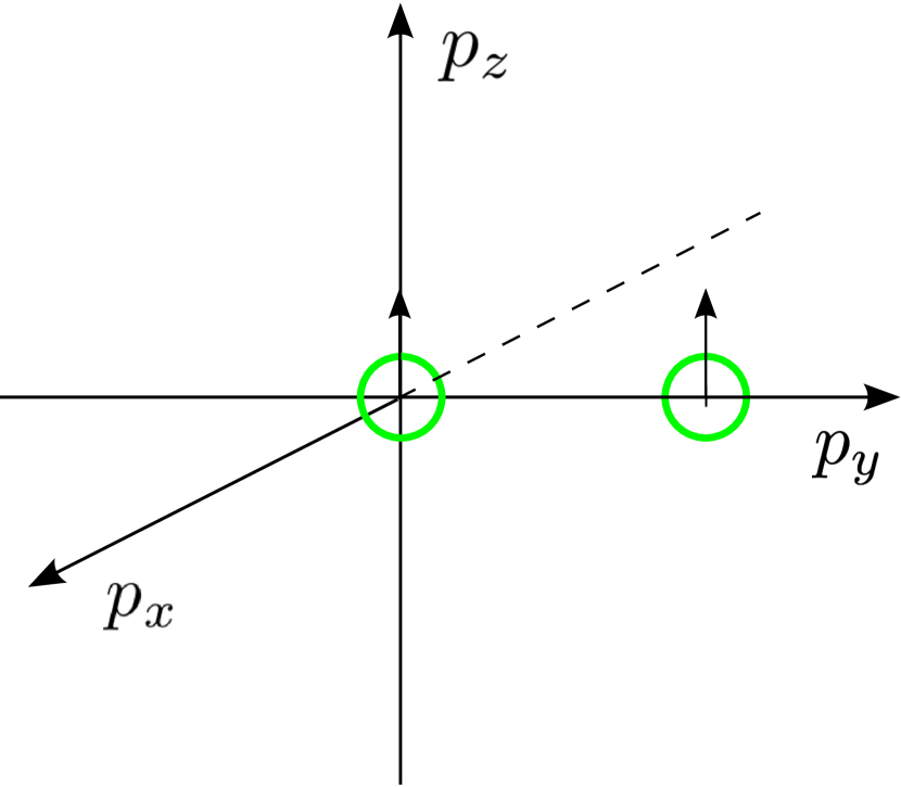
(a)

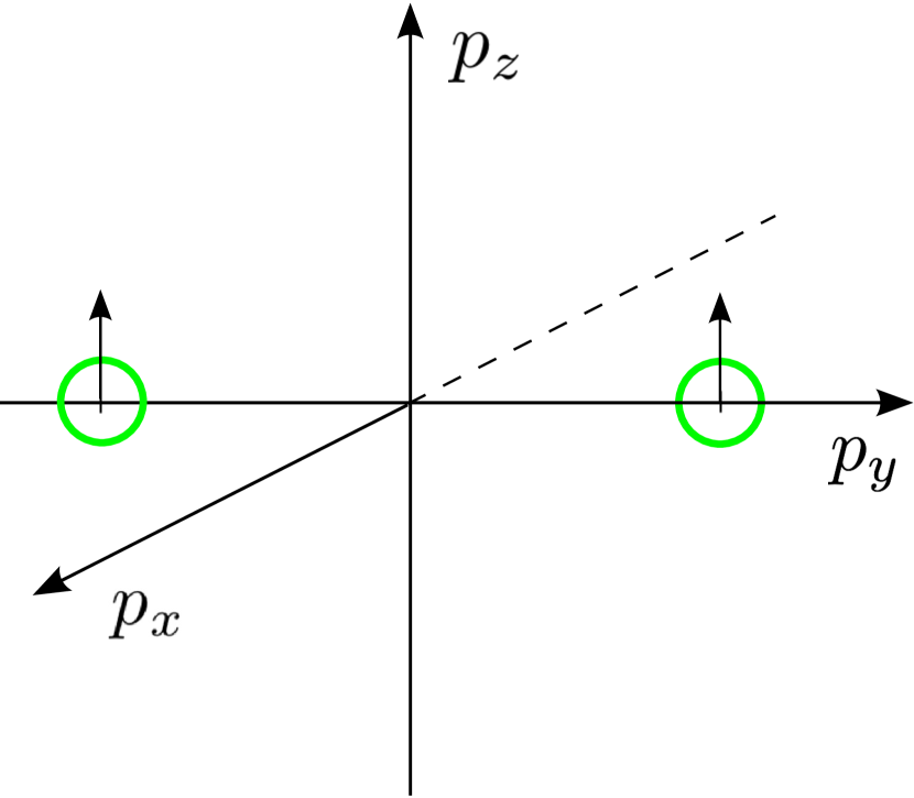
(b)

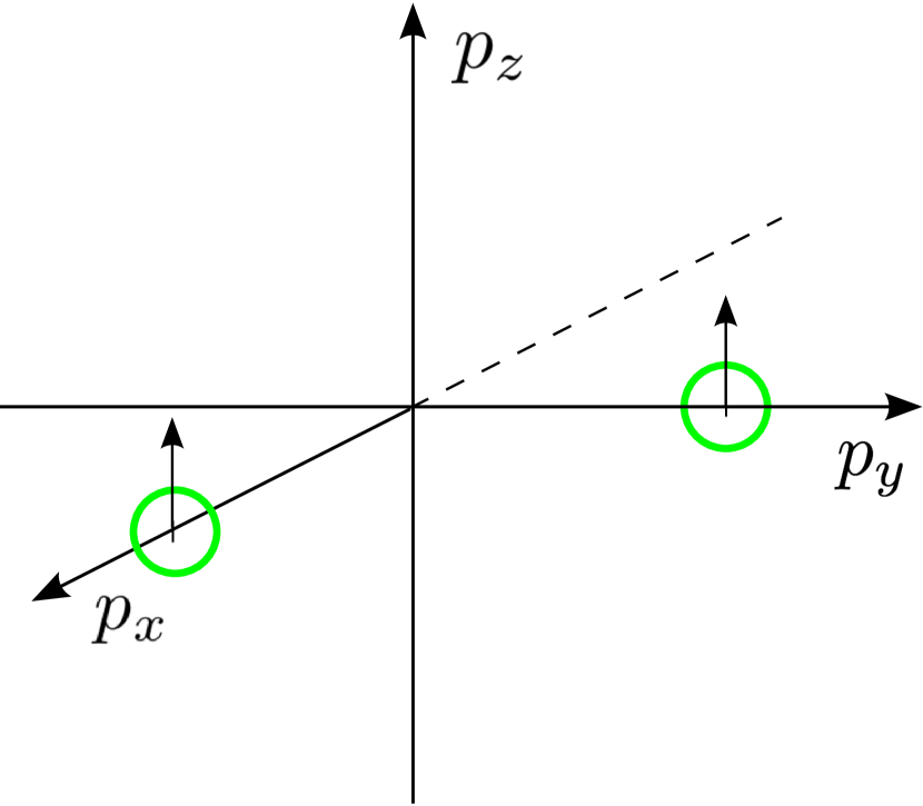
(c)

Figure 2: (Color online.) Schematic illustration. Examples of geometric configurations of Gaussian momenta (green circles) for realizations of different types of rotations on spins, with (a) $R_{i}\otimes\mathbb{1}$, (b) $R_{i}\otimes R_{i}$, (c) $R_{i}\otimes R_{j},i\neq j$. The $z$-projection of the spin field is indicated by an arrow at the Gaussian.

For instance, we saw that $R_{i}\otimes R_{i}$ is instantiated by $R_{Y}\otimes R_{Y}$ when the momenta are given by the product state $\mathop{\left|M_{\Sigma}^{XX}\right\rangle}$ and the boost is in the $z$-direction. Another implementation of the same type is $R_{X}\otimes R_{X}$ when the momenta are again a product but located along the $y$-axis, $\mathop{\left|M_{\Sigma}^{YY}\right\rangle}$, and the boost is in the $z$-direction.

We will next give a few examples of momenta and boost geometries that implement the different types of rotations listed in (VII).

Type $R_{i}\otimes\mathbb{1}$.

In this scenario, only the first particle undergoes rotation. The momentum of the second particle is chosen so that it leaves the spin alone. Denoting such a momentum by $\mathop{\left|0\right\rangle}$, the following pairs of boosts and momenta listed on the left hand side generate rotations given on the right hand side,

$$\Lambda_{z}\,,\mathop{\left|\mathbf{p}_{y},0\right\rangle}\longmapsto R_{X}\otimes\mathbb{1},$$

$$\Lambda_{z}\,,\mathop{\left|\mathbf{p}_{x},0\right\rangle}\longmapsto R_{Y}\otimes\mathbb{1},$$ (41)

$$\Lambda_{y}\,,\mathop{\left|\mathbf{p}_{x},0\right\rangle}\longmapsto R_{Z}\otimes\mathbb{1}.$$

Type $R_{i}\otimes R_{i}$.

For scenarios in which both particles are rotated around the same axis but not necessarily in the same direction, we obtain the following boosts and momenta,

$$\Lambda_{z}\,,\mathop{\left|\mathbf{p}_{y},\mathbf{q}_{y}\right\rangle}\longmapsto R_{X}\otimes R_{X},$$

$$\Lambda_{z}\,,\mathop{\left|\mathbf{p}_{x},\mathbf{q}_{x}\right\rangle}\longmapsto R_{Y}\otimes R_{Y},$$ (42)

$$\Lambda_{y}\,,\mathop{\left|\mathbf{p}_{x},\mathbf{q}_{x}\right\rangle}\longmapsto R_{Z}\otimes R_{Z}.$$

Type $R_{i}\otimes R_{j}$, $i\neq j$.

Scenarios where particles undergo rotations around different axes can be realized by

$$\Lambda_{y}\,,\mathop{\left|\mathbf{p}_{z},\mathbf{q}_{x}\right\rangle}\longmapsto R_{X}\otimes R_{Z},$$

$$\Lambda_{z}\,,\mathop{\left|\mathbf{p}_{y},\mathbf{q}_{x}\right\rangle}\longmapsto R_{X}\otimes R_{Y},$$ (43)

$$\Lambda_{x}\,,\mathop{\left|\mathbf{p}_{z},\mathbf{q}_{y}\right\rangle}\longmapsto R_{Y}\otimes R_{Z}.$$

These scenarios admit an obvious generalization. By choosing momenta and boosts appropriately, one can consider single particle rotations around an arbitrary axis $\mathbf{n}=(n_{x},n_{y},n_{z})$. This leads to combinations of generic rotations $R_{\mathbf{n}_{1}}\otimes R_{\mathbf{n}_{2}}$ for two particle systems, opening up a wide avenue of research. However, when surveying the landscape for the first time, we would like to keep the situation tractable by confining attention to the cases listed above and leave a more general approach for another occasion.

VIII Spin state and its visualization

We will next characterize the spin state of the system. Most previous work has focussed on the Bell states,

$$\mathop{\left|\Phi_{\pm}\right\rangle}=\frac{1}{\sqrt{2}}\left(\mathop{\left|00\right\rangle}\pm\mathop{\left|11\right\rangle}\right),\quad\mathop{\left|\Psi_{\pm}\right\rangle}=\frac{1}{\sqrt{2}}\left(\mathop{\left|01\right\rangle}\pm\mathop{\left|10\right\rangle}\right),$$ (44)

the maximally entangled bipartite states of two level systems. Understanding their behavior in relativity is important for quantum information and we will follow suit in this paper . As regards the geometric configuration, we will assume throughout that the spins are aligned with the $z$-axis irrespective of the direction of the boost. We adopt the convention that $\mathop{\left|0\right\rangle}$ signifies the ‘up’ spin and $\mathop{\left|1\right\rangle}$ the ‘down’ spin.

In order to gain a better understanding of the state change of a single qubit, one commonly uses visualization in terms of the Bloch sphere. Visualization of two qubits, however, is in general impossible since one needs $15$ real parameters to characterize the density matrix. However, some cases still allow for a representation in three space, for instance when the state is restricted to evolve in a subspace of few dimensions. Fortunately this turns out to be the case for our system.

It is useful to work in the Hilbert-Schmidt space of operators $B(\mathcal{H})$, defined on the Hilbert space $\mathcal{H}$ with $\text{dim}=N$ Bengtsson and Życzkowski (2006). $B(\mathcal{H})$ becomes a Hilbert space of $N^{2}$ complex dimensions when equipped with a scalar product defined as $\langle A|B\rangle=\text{Tr}(A^{\dagger}B)$, with $A,B\in B(\mathcal{H})$, where the squared norm is $\|A\|^{2}=\text{Tr}(A^{\dagger}A)$. The vector space of Hermitian operators is an $N^{2}$ real-dimensional subspace of Hilbert-Schmidt space which can be coordinatized using a basis that consists of identity operator and the generators of $\mathrm{SU}(N)$. For a qubit $N=2$ and we obtain the familiar Bloch ball. For a bipartite qubit system $N=4$, $B(\mathcal{H})=B(\mathcal{H}_{A})\otimes B(\mathcal{H}_{B})$ where $\mathcal{H}_{i}$ is the single particle space, and we can use a basis whose elements are the tensor products $\{\mathbb{1}\otimes\mathbb{1},\mathbb{1}\otimes\bm{\sigma},\bm{\sigma}\otimes\mathbb{1},\bm{\sigma}\otimes\bm{\sigma}\}$, where $\bm{\sigma}=\left(\sigma_{x},\sigma_{y},\sigma_{z}\right)$ is the vector of Pauli operators. The density operator for a $2\times 2$ dimensional system can be written in the general form,

$$\rho=\frac{1}{4}\left(\mathbb{1}\otimes\mathbb{1}+\mathbf{r}\bm{\sigma}\otimes\mathbb{1}+\mathbb{1}\otimes\mathbf{s}\bm{\sigma}+\sum_{i,j}t_{ij}\sigma_{i}\otimes\sigma_{j}\right),$$ (45)

where the coefficients $\mathbf{r}=(r_{x},r_{y},r_{z})$, $\mathbf{s}=(s_{x},s_{y},s_{z})$ and $t_{ij}$, $i,j\in\{x,y,z\}$ are the expectation values of the operators $\bm{\sigma}\otimes\mathbb{1}$, $\mathbb{1}\otimes\bm{\sigma}$ and $\sigma_{i}\otimes\sigma_{j}$.

For the projectors on the Bell states $s_{i}=r_{i}=0$ and the matrix $t_{ij}$ is diagonal. This implies we only need to consider the values of diagonal components $t_{ii}$ which constitute a vector in $3$-dimensional space, allowing us to represent the states in Euclidean three space Bertlmann et al. (2002). The Bell states correspond to vectors,

$$t_{\Phi_{+}}=\left(1,-1,\phantom{-}1\right),\quad\quad t_{\Phi_{-}}=\left(-1,\phantom{-}1,\phantom{-}1\right),$$

$$t_{\Psi_{+}}=\left(1,\phantom{-}1,-1\right),\quad\quad t_{\Psi_{-}}=\left(-1,-1,-1\right),$$ (46)

which, in turn, correspond to the vertices of a tetrahedron $\mathcal{T}$ in Fig. 3. By taking convex combinations of these, one obtains further diagonal states; the set of all such states is called Bell-diagonal and is represented by the (yellow) tetrahedron $\mathcal{T}$ in Fig. 3.

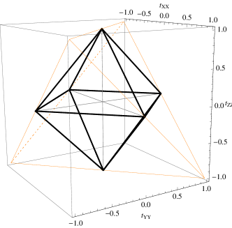
Figure 3: (Color online.) The geometry of Bell diagonal states. The vertices of the tetrahedron $\mathcal{T}$ (thin yellow lines) correspond to the four Bell states $\mathop{\left|\Phi_{+}\right\rangle}$, $\mathop{\left|\Phi_{-}\right\rangle}$, $\mathop{\left|\Psi_{+}\right\rangle}$, and $\mathop{\left|\Psi_{-}\right\rangle}$. Convex combinations of projectors on the Bell states, the Bell diagonal states, lie on or in the tetrahedron (thick black lines). A Bell diagonal state is separable iff it lies in the double pyramid formed by the intersection of the tetrahedron $\mathcal{T}$ and its reflection through the origin $\mathcal{-T}$.

The set of separable states forms a double pyramid, an octahedron, in the tetrahedron. The octahedron is given by the intersection of $\mathcal{T}$ with its reflection through the origin, $-\mathcal{T}$. The maximally mixed state $\frac{1}{4}\mathbb{1}_{4}$ has coordinates $(0,0,0)$ and it lies at the origin. The entangled states are located outside the octahedron in the cones of the tetrahedron, see Fig. 3.

We can now visualize the behavior of spin by calculating the coefficients $t_{ii}$ under a given rotation as a function of rapidity $\xi$,

$$t(\xi)=\left(t_{xx},t_{yy},t_{zz}\right),$$ (47)

where

$$t_{ii}=\text{Tr}\!\left[\rho^{\Lambda}_{S}(\xi)\,\sigma_{i}\otimes\sigma_{i}\right],\quad i\in\{x,y,z\},$$ (48)

and $\rho^{\Lambda}_{S}(\xi)$ is the boosted spin state. The resulting set of three vectors

$$\Gamma\!\left[\rho^{\Lambda}_{S}(\xi)\right]=\{t(\xi)\;|\;\xi\in[0,\xi_{\text{max}}]\}$$ (49)

we call an orbit of a given initial state. It can be represented as a curve in three space in the manner described above.

IX Product momenta $f_{\mathrm{EPRB}}$

We begin by considering product momenta of the simplest form

$$f_{\mathrm{EPRB}}(\mathbf{p},\mathbf{q},\mathbf{p}_{0},\mathbf{q}_{0})=\left[N(\sigma)\right]^{-\frac{1}{2}}g\!\left(\mathbf{p},\mathbf{p}_{0}\right)g\!\left(\mathbf{q},-\mathbf{p}_{0}\right),$$ (50)

which represent the EPR–Bohm scenario where two particles move in opposite directions $\mathbf{p}_{0}$ and $-\mathbf{p}_{0}$. Early discussion focussed on momentum delta states and concluded that spin entanglement of a Bell state was left invariant Lorentz boosts Alsing and Milburn (2002); Terashima and Ueda (2003). We reproduce the case of delta momentum by approximating it with a narrow Gaussian of width $\sigma/m=1$. In order to study wavepackets of larger widths, we also calculate $\sigma/m=2,4$. The concurrence for all three cases is shown in Fig. 4. Unfortunately, the spin orbit cannot be visualized since it is not Bell diagonal.

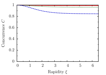
Figure 4: (Color online.) Spin concurrence for Gaussian momenta $f_{\mathrm{EPRB}}$ with $\sigma/m=1,2,4$ and centers of Gaussians lying on the $x$-axis at $\pm\mathbf{p}_{X0}=(\pm 17.13,0,0)$. Data for $\sigma/m=1$ is shown with the solid red line, $\sigma/m=2$ green dotted line and $\sigma/m=4$ blue dot-dashed line.

The narrow momenta $\sigma/m=1$ which approximate the delta state confirm the results obtained by Alsing and Milburn (2002); Terashima and Ueda (2003), namely, that boosts leave the entanglement of a maximally entangled Bell state invariant. Larger widths, however, show a decrease of entanglement, which grows with the width and magnitude of the boost.

To analyze the behavior, we will resort to the simple discrete model used above when discussing the relation between momenta and rotations. We can approximate the narrow momenta $\sigma/m=1$ by a single momentum term and write the total state of the boosted particle in discrete form as in (VII),

$$\mathop{\left|\Psi^{\Lambda}\right\rangle} =\mathop{\left|\Lambda_{z}\mathbf{p}_{0},-\Lambda_{z}\mathbf{p}_{0}\right\rangle}\,D\!\left[W(\Lambda_{z},\mathbf{p}_{0})\right]$$

$$\phantom{AAAAAAAA}\otimes D\!\left[W(\Lambda_{z},-\mathbf{p}_{0})\right]\mathop{\left|\Phi_{+}\right\rangle}.$$ (51)

This shows that the boost generates a local unitary transform of the form $D_{1}\otimes D_{2}$ on the spin state $\mathop{\left|\Phi_{+}\right\rangle}$. Since the degree of entanglement of any Bell state is left invariant by such a transform, Lorentz boosts do not change the entanglement between spins in this case.

Systems with widths $\sigma/m=2,4$, however, display loss of spin entanglement. This is because they cannot be modeled using a single momentum term. A larger width means that, in analogy with Eq. (VII), the discrete model now consists of several momenta and the boosted state involves many rotation operators acting on the spin state. Calculating the boosted spin state, we obtain

$$\rho_{\Phi+}^{\Lambda} =\sum_{\mathbf{p},\mathbf{q}}|f_{\mathrm{EPRB}}(\mathbf{p},\mathbf{q})|^{2}D\!\left[W(\Lambda,\mathbf{p},\mathbf{q})\right]\rho_{\Phi+}\,D^{\dagger}\!\left[W(\Lambda,\mathbf{p},\mathbf{q})\right],$$ (52)

where $f_{\mathrm{EPRB}}$ is centered at $\mathbf{p}_{0}$ and $-\mathbf{p}_{0}$, respectively, $\rho_{\Phi+}=\mathopen{}\left|{\Phi_{+}}\right\rangle\!\left\langle{\Phi_{+}}\right|$, and we have abbreviated $D\!\left[W(\Lambda,\mathbf{p},\mathbf{q})\right]\equiv D\!\left[W(\Lambda,\mathbf{p})\right]\otimes D\!\left[W(\Lambda,\mathbf{q})\right]$. The final spin state $\rho_{\Phi+}^{\Lambda}$ is in general a mixed state whose entanglement has changed as a result of the boost. Based on the discrete model, one would expect that larger widths lead to bigger changes when rapidity increases because, roughly, the rotations generated by different momenta diverge more than in the case of narrow momenta. Indeed, the plots of $\sigma/m=2,4$ in Fig. 4, which have been obtained using numerical methods, confirm this intuition.

X Product momenta $f_{\Sigma}$

In this section we will focus on spin rotations generated by product momenta of the form $f_{\Sigma}$. In order to study the maximum range of phenomena that Lorentz boosts can exhibit we will choose boost scenarios with large boost angles and momenta so that the spins undergo large TWR when boosts approach the speed of light. To this end, we will assume that the centers of the Gaussians are given by geometric vectors $\pm\mathbf{p}_{X0}=(\pm 17.13,0,-98.5)$ and $\pm\mathbf{p}_{Y0}=(0,\pm 17.13,-98.5)$, see Fig. 5.

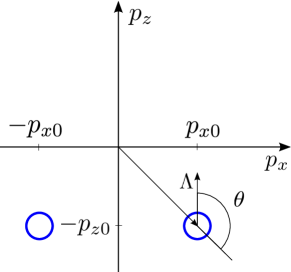
Figure 5: (Color online.) Schematic illustration of a boost at a large angle $\theta$. Gaussian momenta (shown as blue circles) are located at $(\pm p_{x0},0,-p_{z0})$. Boost $\Lambda$ is in the positive $z$-direction.

This corresponds to the maximum TWR of $163^{\circ}$ at large boosts $\xi=6.5$.

X.1 Case $R_{i}\otimes\mathbb{1}$

It is not easy to implement rotations of type $R_{i}\otimes\mathbb{1}$ in the continuous regime as long as we are concerned with the physical situation where the observer moves relative to both particles. The problem lies in realizing the identity map. Even if we find a scenario where boosts leave alone a momentum given by a delta state, the non-zero width of the wave packet guarantees that this will not apply to the whole wave packet. Some parts of the wave packet will necessarily induce non-trivial transformations on the spin state as we learned in studying the continuous momentum models of a single particle in Palge and Dunningham (2012). We will thus adopt the strategy of constructing a model that approximates the identity map to as high a degree as possible by minimizing the effect of boost on the spin of the second particle.

Above we fixed the boost to be always in the $z$-direction. In order to realize the $R_{i}\otimes\mathbb{1}$ rotations, we will take the momentum of the first particle to lie in the $zx$-plane with $\pm\mathbf{p}_{0}=\pm\mathbf{p}_{X0}$, while the momentum of the second particle is located at the origin of the $xy$-plane with the $z$-component equal to that of the first particle, $\mathbf{q}_{0}=(0,0,-98.5)$. Since the momentum of the second particle is aligned with the direction of the boost, the resulting rotation of the spin field approximates the identity map.

We plot the orbit of the spin state along with its concurrence in Fig. 6.

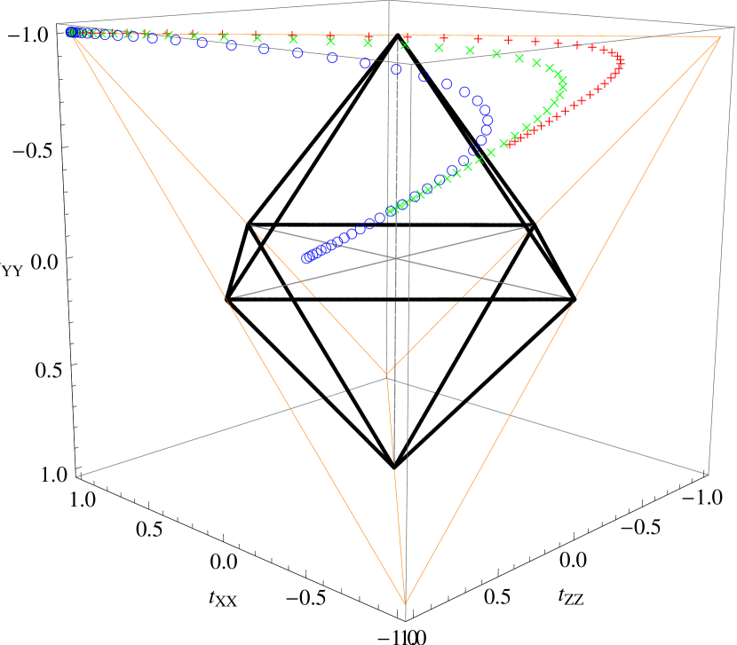
(a)

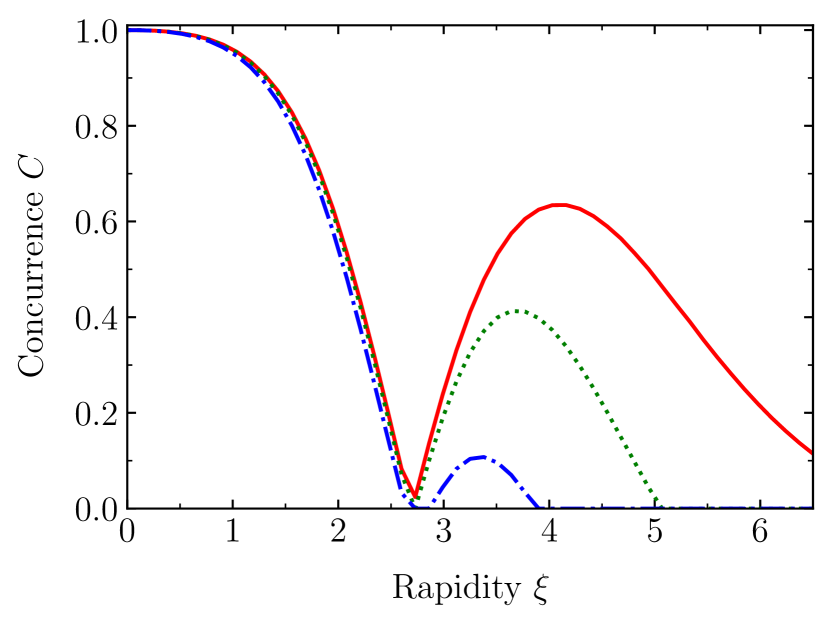
(b)

Figure 6: (Color online.) Spin (a) orbit and (b) concurrence under $R_{i}\otimes\mathbb{1}$ for Gaussian momenta $f_{\Sigma}$ with $\sigma/m=1,2,4$. Data for $\sigma/m=1$ is shown with (a) the red “+” and (b) the red solid line, $\sigma/m=2$ with (a) the green “$\times$” and (b) the green dotted line, $\sigma/m=4$ with (a) the blue “$\bigcirc$” and (b) the blue dot-dashed line. (a) Initial state $\mathop{\left|\Phi_{+}\right\rangle}$ corresponds to vertex $(1,-1,1)$.

It is evident that visualization of the orbit provides valuable insight into the behavior of the state, as well as explaining the behavior of entanglement. Let us begin by considering the case $\sigma/m=1$, shown red in Fig. 6(a). Initially the state is at rest, represented by the state $\mathop{\left|\Phi_{+}\right\rangle}$ at the vertex $(1,-1,1)$. When boosts begin to increase, the state moves towards the center of the face, reaching a separable state $(0,-1,0)$ at about $\xi=2.7$. Correspondingly, the concurrence initially takes value $1$, decreasing monotonically with the increase of boosts. It vanishes at about $\xi=2.7$ when the state hits the separable region.

When boosts become larger than $2.7$, the spin of the first particle is rotated even further, and the system becomes again entangled, with the orbit moving towards the vertex $(-1,-1,-1)$ which represents the Bell state $\mathop{\left|\Psi_{-}\right\rangle}$. However, the revival of entanglement stops short of reaching the value $0.64$ for concurrence. Concurrence starts to decrease when $\xi$ becomes larger than $4.16$.

While the states with $\sigma/m=2$ and $\sigma/m=4$ display similar qualitative behavior, their orbits lie increasingly more in the region of separable states as $\sigma/m$ becomes larger, see Fig. 6(a). As a consequence, the revival of concurrence becomes less pronounced, recovering only briefly for $\sigma/m=4$ in the interval $\xi\in[2.9,3.9]$ and vanishing thereafter as the state enters the octahedron of separable states.

X.2 Case $R_{i}\otimes R_{i}$

To implement the type of rotation where both particles undergo rotation around the same axis, the momenta $\mathbf{p}_{0}$ and $\mathbf{q}_{0}$ need to lie in the same boost plane. Since the boost is in the $z$-direction, we will assume that the Gaussians are centered at the geometric vectors $\pm\mathbf{q}_{0}=\pm\mathbf{p}_{0}=\pm\mathbf{p}_{X0}$, realizing the rotation $R_{Y}\otimes R_{Y}$. Plots of the orbits and concurrence are shown in Fig. 7.

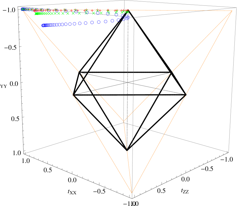
(a)

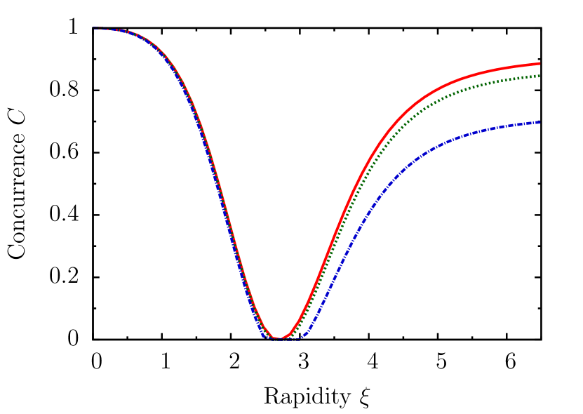
(b)

Figure 7: (Color online.) Spin (a) orbit and (b) concurrence under $R_{i}\otimes R_{i}$ for Gaussian momenta with $\sigma/m=1,2,4$. Product momenta are given by $f_{\Sigma}$. Data for $\sigma/m=1$ is shown with (a) the red “+” and (b) the red solid line, $\sigma/m=2$ with (a) the green “$\times$” and (b) the green dotted line, $\sigma/m=4$ with (a) the blue “$\bigcirc$” and (b) the blue dot-dashed line. (a) Initial state $\mathop{\left|\Phi_{+}\right\rangle}$ corresponds to vertex $(1,-1,1)$.

Let us first consider $\sigma/m=1$. At first, the effect of boosts is quite similar to the previous case. When rapidity is smaller than $2.6$, the state is mapped into a mixture of itself and the projector onto $\mathop{\left|\Psi_{-}\right\rangle}$, moving along an orbit that connects the two states. At about $\xi=2.6$, the boosted observer sees a separable state. However, for larger boosts the orbit differs from the previous case as the state moves back along the same path towards the rest frame state. The concurrence mimics this pattern by first decreasing monotonically until $\xi=2.6$, and then increasing to almost maximal entanglement for large boosts $\xi>6$.

The orbits for $\sigma/m=2$ and $\sigma/m=4$ diverge from this behavior, with the disagreement growing larger as the width increases. This is to be expected since larger Gaussians contain spins some of which undergo less and others more rotation than spins at the centre of the wave packet, thereby causing the spin state to be a mixed state. Larger values of $\sigma/m$ lead in general to a higher degree of mixedness of the boosted state, and the effect becomes more pronounced at extremely large boosts: at $\xi=6.5$, the boosted state with $\sigma/m=4$ is closer to the centre of the octahedron than the states with lower $\sigma/m$.

X.3 Case $R_{i}\otimes R_{j}$

In order to realize scenarios where particles undergo rotations around different axis, the centers of Gaussians need to lie in different boost planes. With the boost in the $z$-direction, we will choose $\pm\mathbf{p}_{0}=\pm\mathbf{p}_{Y0}$ and $\pm\mathbf{q}_{0}=\pm\mathbf{p}_{X0}$, which means that the spin state is rotated by $R_{X}\otimes R_{Y}$. The orbits and concurrence are shown in Fig. 8.

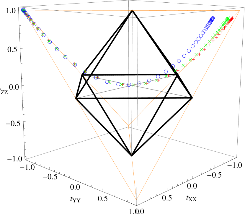
(a)

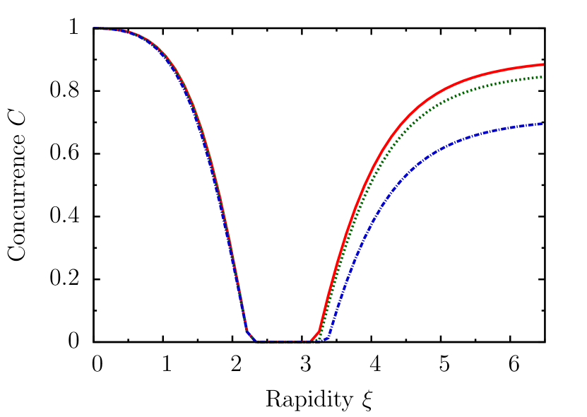
(b)

Figure 8: (Color online.) Spin (a) orbit and (b) concurrence under $R_{i}\otimes R_{j}$, $i\neq j$ for Gaussian momenta with $\sigma/m=1,2,4$. Product momenta are given by $f_{\Sigma}$. Data for $\sigma/m=1$ is shown with (a) the red “+” and (b) the red solid line, $\sigma/m=2$ with (a) the green “$\times$” and (b) the green dotted line, $\sigma/m=4$ with (a) the blue “$\bigcirc$” and (b) the blue dot-dashed line. (a) Initial state $\mathop{\left|\Phi_{+}\right\rangle}$ corresponds to vertex $(1,-1,1)$.

Spin behavior under mixed rotations is quite different from the two previous ones. Let us begin by considering $\sigma/m=1$. The state follows an orbit that has the shape of a curve starting at vertex $(1,-1,1)$ and evolving towards the origin, reaching it at about $\xi=2.7$. The second half of the orbit displays a symmetric shape. The state moves along a curve towards the vertex $(-1,1,1)$ which represents the Bell state $\mathop{\left|\Phi_{-}\right\rangle}$, almost reaching it when $\xi=6.5$.

It is interesting that the spins become briefly separable in the interval $\xi\in[2.2,3.2]$. While this might look puzzling if one only had access to the behavior of concurrence, the plot of orbits gives us deeper insight into what is happening. The spin state evolves in the plane that intersects the octahedron of separable states, entering the octahedron when $\xi=2.2$ and moving along a path towards the maximally mixed state $\frac{1}{4}\mathbb{1}_{4}$ represented by $(0,0,0)$. At $\xi=2.73$ the moving observer sees a maximally mixed state. When the boosts become even larger, the entanglement revives again, becoming non-zero for rapidities greater than $\xi=3.2$, which corresponds to the point where the state leaves the octahedron.

As above, we observe the generic feature that states with larger widths deviate from this behavior at higher values of rapidity and the difference grows with $\sigma/m$. While the orbits are fairly similar up to the maximally mixed state, they start to diverge soon thereafter, with the momenta $\sigma/m=4$ showing least gain in concurrence. Correspondingly, the latter state follows an orbit in the set of states with lower degree of entanglement.

XI Axis centered Gaussians

One of the first studies of two particle entanglement in relativity was carried through in the seminal paper Gingrich and Adami (2002), which focussed on systems whose momenta were given by Gaussians centered at the origin. In this section, we will study scenarios which are more general, involving momenta that are centered on the $z$-axis. In particular, in the first scenario the Gaussian momenta are shifted in the positive direction, $\mathbf{p}_{0}=(0,0,4)$, in the second in the negative direction, $\mathbf{p}_{0}=(0,0,-4)$, and in the third we reproduce the origin centered momenta of Gingrich and Adami (2002), see Fig. 9. Fourthly, we will consider Gaussians that are far away from the origin, $\mathbf{p}_{0}=(0,0,-98.5)$, and thus likely to induce large rotations on the spins.

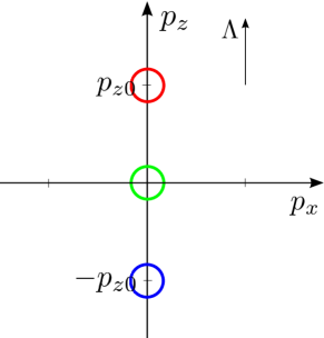
Figure 9: (Color online.) Schematic illustration of axis centered Gaussians shifted in the positive (top red circle) and negative (bottom blue circle) direction, and centered at the origin (middle green circle). Boost $\Lambda$ is in the positive $z$-direction.

Plots for $\sigma/m=1$ and $\sigma/m=4$ with the first three momenta are shown in Fig. 10 and 11. The results of Gingrich and Adami (2002) correspond to the Gaussian momenta which have $\sigma/m=1$ and $\sigma/m=4$ and where the momenta are centered at $(0,0,0)$.

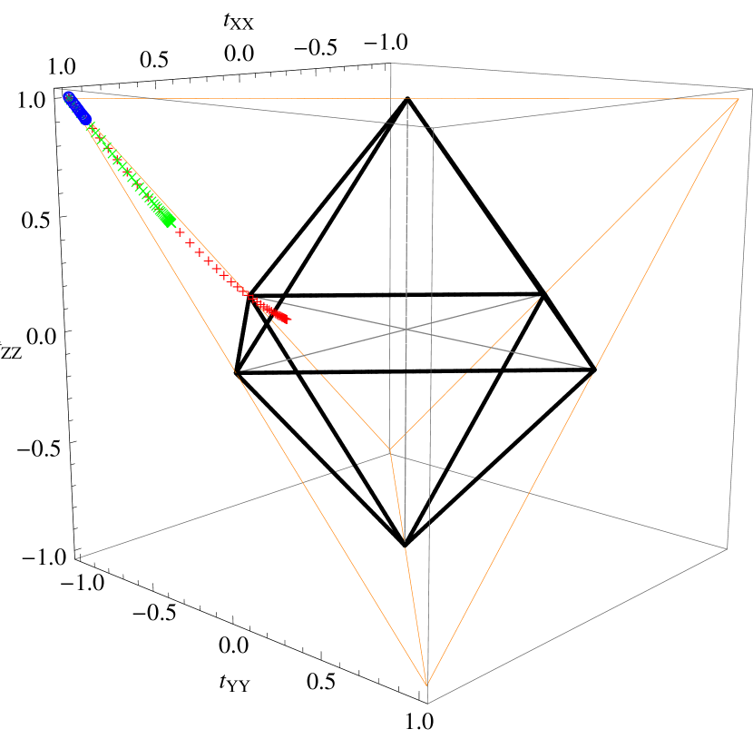
(a)

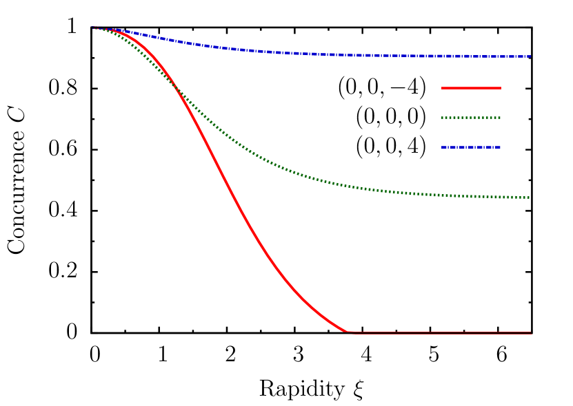
(b)

Figure 10: (Color online.) Spin (a) orbit and (b) concurrence for origin centered Gaussian momenta with $\sigma/m=1$. Data for $(0,0,-4)$ is shown with (a) the red “+” and (b) the red solid line, $(0,0,0)$ with (a) the green “$\times$” and (b) the green dotted line, $(0,0,4)$ with (a) the blue “$\bigcirc$” and (b) the blue dot-dashed line. (a) Initial state $\mathop{\left|\Phi_{+}\right\rangle}$ corresponds to vertex $(1,-1,1)$.

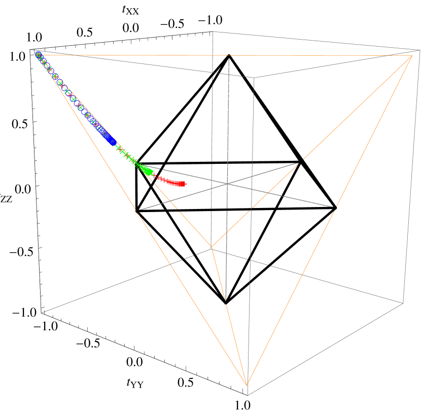
(a)

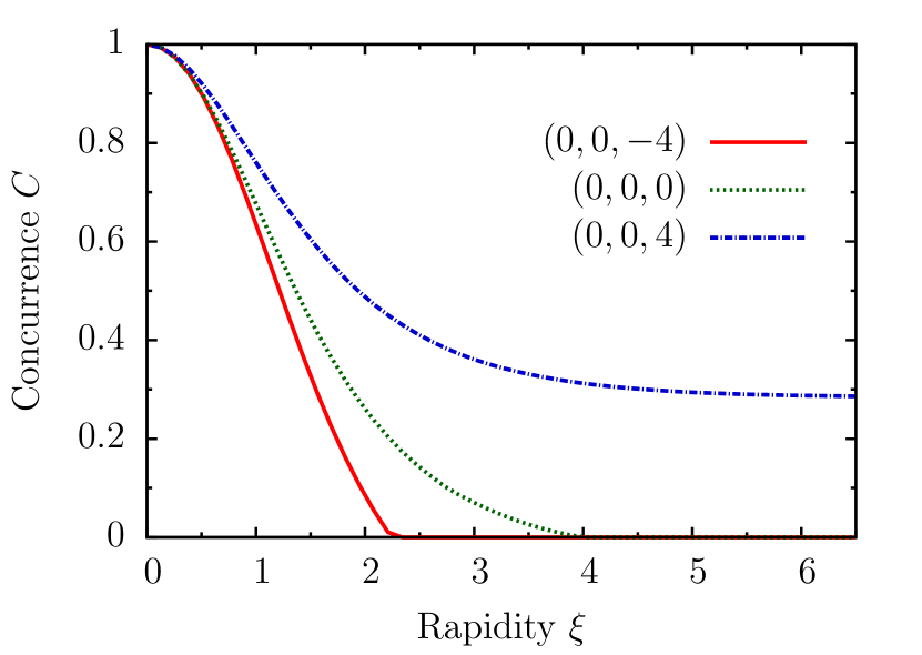
(b)

Figure 11: (Color online.) Spin (a) orbit and (b) concurrence for origin centered Gaussian momenta with $\sigma/m=4$. Data for $(0,0,-4)$ is shown with (a) the red “+” and (b) the red solid line, $(0,0,0)$ with (a) the green “$\times$” and (b) the green dotted line, $(0,0,4)$ with (a) the blue “$\bigcirc$” and (b) the blue dot-dashed line. (a) Initial state $\mathop{\left|\Phi_{+}\right\rangle}$ corresponds to vertex $(1,-1,1)$.

Let us consider first $\sigma/m=1$. Note that we have changed tack a little. Whereas in the previous sections we kept the center of the Gaussian momentum fixed, here we keep its width fixed and change the coordinate of the center. The differences between the three scenarios in Fig. 10 are quite dramatic. While $\mathbf{p}_{0}=(0,0,4)$ shows relatively little decrease of entanglement with the concurrence saturating at $0.9$ for large boosts $\xi=6.5$, the system with $\mathbf{p}_{0}=(0,0,0)$ loses more than half of the entanglement and saturates at $0.45$. The third one with momentum at $\mathbf{p}_{0}=(0,0,-4)$ displays a steep decrease of concurrence, with the entanglement vanishing altogether for rapidities $\xi>3.75$. Momenta with $\sigma/m=4$ exhibit similar features, albeit with much steeper decreases of concurrence. Even for $\mathbf{p}_{0}=(0,0,4)$, the boosted state has only about $0.3$ of the original degree of entanglement at large boosts, and $\mathbf{p}_{0}=(0,0,-4)$ vanishes already at $\xi=2.2$. The corresponding orbits follow a trajectory which evolve towards the base of the upper pyramid of separable states, see Figs. 10(a) and 11(a). All the orbits follow the same path, the only difference lying in that some stop sooner than others. The latter is determined by the location and width of the Gaussian. Momenta whose centers are shifted farther in the negative direction and have larger widths correspond to the final states closer to the center of the octahedron and exhibit, consequently, a quicker and steeper decline of the concurrence.

XI.1 Comparison with single particle

It is instructive to discuss how these results relate to a single particle system with axis centered momenta Palge and Dunningham (2012). At first sight it might seem that the single and two particle systems are not directly comparable because the entanglements in question are between different degrees of freedom: spin–momentum entanglement in case of the single particle versus spin–spin in case of two particles. Correspondingly, the structure of maps that change entanglement in each case as well as the initial states of systems are different too. However, despite this a number of analogies are manifest and we will argue that this is no coincidence. Both systems show features which can be explained using the properties of TWR.

Firstly, the two particle scenario with $\mathbf{p}_{0}=(0,0,4)$, which involves momenta in the direction of boost, displays less pronounced changes of entanglement than the one with a Gaussian centered at $\mathbf{p}_{0}=(0,0,-4)$, which has momenta opposite to the direction of boost. As discussed in Palge and Dunningham (2012), this originates in the sensitivity of TWR to the angle between boosts. Smaller boost angles lead to smaller TWR, which in turn result in smaller changes of entanglement. Secondly, in analogy with the single particle, Gaussians with larger widths show in general more rapid changes of concurrence. This can be traced back to the dependence of TWR on the magnitude of the boost. A Gaussian with a larger width is equivalent to a system undergoing a larger boost, which in turn causes a larger TWR angle. Thirdly, both single and two particle systems exhibit saturation, which comes from the fact that the TWR achieves a maximum value, which for a given boost angle is determined by the smaller boost.

XI.2 Large momenta

Let us next turn to the case of large momenta $\mathbf{p}_{0}=(0,0,-98.5)$. Plots for $\sigma/m=1,2,4,8$ are shown in Fig. 12.

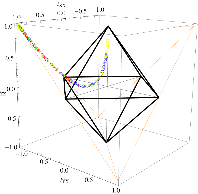
(a)

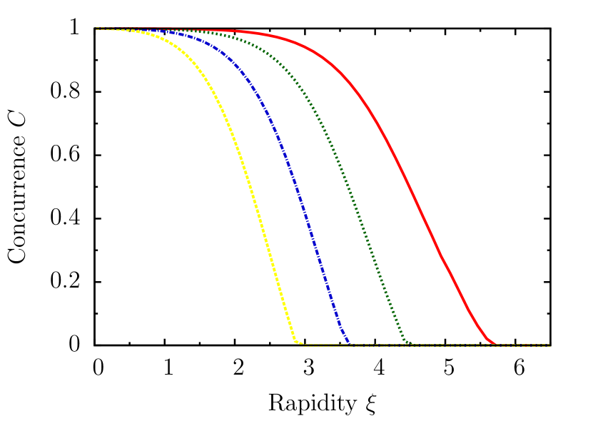
(b)

Figure 12: (Color online.) Spin (a) orbit and (b) concurrence for axis centered Gaussian momenta $f_{C}$ with $\sigma/m=1,2,4,8$ and $\mathbf{p}_{0}=(0,0,-98.5)$. Data for $\sigma/m=1$ is shown with (a) the red “+” and (b) the red solid line, $\sigma/m=2$ with (a) the green “$\times$” and (b) the green dotted line, $\sigma/m=4$ with (a) the blue “$\bigcirc$” and (b) the blue dot-dashed line, $\sigma/m=8$ with (a) the yellow “$\Box$” and (b) the yellow dotted leftmost line. (a) Initial state $\mathop{\left|\Phi_{+}\right\rangle}$ corresponds to vertex $(1,-1,1)$.

Interestingly, and contrary to what one might expect based on the findings so far, entanglement declines more slowly than in the previous scenarios. For instance, states with $\sigma/m=1$ remain nearly maximally entangled for rapidities up to about $2$ and decohere thereafter, but this occurs later than with the momenta $\mathbf{p}_{0}=(0,0,-4)$, which on the face of it generate smaller rotation angles than the extreme momenta $\mathbf{p}_{0}=(0,0,-98.5)$. However, on closer examination such puzzling behavior can be again explained using the properties of TWR. Instead of a Gaussian, let us think of a rough, simple model consisting of discrete momenta in the $xz$-plane as depicted in Fig. 13. We know that larger momenta generate larger rotation angles, but their amplitude is smaller, so for the sake of argument, let us assume that the Gaussian is represented by two momenta at the distance of $0.75$ its width.

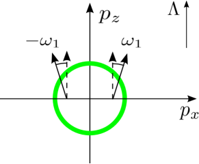
Figure 13: Schematic representation of an origin centered Gaussian spin field.

We will next argue that concurrence changes more rapidly for the Gaussian centered at or close to the origin than for the one centered at the very large momentum $(0,0,-98.5)$. The key is to realize that the boost angle $\theta$ is $\pi/2$ for the origin centered Gaussian, while it is larger, about $170^{\circ}$ or $2.97$ rad, for the Gaussian at $(0,0,-98.5)$. In Fig. 1, which describes the dependence of TWR angle on boost angle and rapidity, these states lie, respectively, in the middle and almost at the right end of the horizontal axis. Boosting the system means we keep $\theta$ fixed and move towards the back of the surface representing the TWR angle for the given $\theta$ and $\xi$. Now for $\theta=\pi/2$, the rotation grows initially faster than for $\theta=2.85$, meaning that the concurrence of the origin centered Gaussian changes sooner than the one at the extremely large momentum. However, as rapidity grows even larger, the rotation increases rapidly for $\theta=2.85$, leading to the decrease of concurrence as seen in Fig. 12. The decrease becomes steeper as width increases, as is to be expected since larger width means we move towards slightly lower values of $\theta$ in Fig. 1 which cause faster rotations and hence quicker drop of concurrence. Along the same lines, for Gaussians at $(0,0,-4)$ which are relatively close to the origin in comparison to $(0,0,-98.5)$, $\theta$ is slightly but not significantly larger than $\pi/2$, still leading to faster initial increase than for the extremely large momenta.

To substantiate these qualitative considerations with a rough numerical model, we plot the dependence of TWR on rapidity for four delta momenta in Fig. 14.

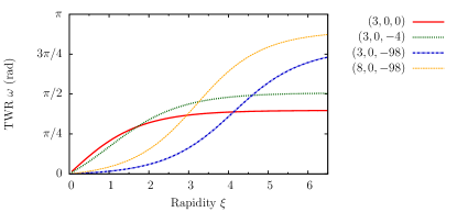
Figure 14: (Color online.) TWR for axis centered Gaussians in different geometries.

The first one at $(3,0,0)$ corresponds to the origin centered Gaussian and the second $(3,0,-4)$ to the one close to the origin. The third $(3,0,-98)$ represents a distribution with the same width at the extreme momentum and the fourth $(8,0,-98)$ corresponds to a Gaussian with larger width at the extreme momentum. The qualitative behavior of TWR and hence of concurrence follows the pattern we have just outlined. Quantitatively, however, our discrete considerations in the 2D setting cannot accurately represent the more complex workings of realistic 3D Gaussian wave packets. The model in Fig. 14 does not reproduce the precise numerical values for concurrence in Figs. 10, 11 and 12.

To summarize, the claim we make is that the behavior of a Gaussian system can be understood qualitatively, and to some extent even quantitatively, using a rather simple model involving a small sample of discrete (or very narrow Gaussian) momenta.

XII Product momenta $f_{\times}$

We will next study product momenta of the form $f_{\times}$. Above we introduced them as a generalization of $f_{\Sigma}$. In this section, however, we will show that they serve another purpose as well: in many cases, they can be used to model the axis centered Gaussians of the previous section. This has mainly the conceptual importance of providing a rough and ready explanation of how the axis centered systems behave. The practical use of this exercise is somewhat limited since we will not provide systematic methods for finding the exact parameters that characterize such models.

We start by noting that the state $f_{\times}$ admits only two types of rotations: $R_{i}\otimes\mathbb{1}$ and a mixture of $R_{i}\otimes R_{i}$ and $R_{i}\otimes R_{j}$. We will forgo the former type since it is not interesting from the point of view of comparison with the axis centered systems. To discuss the latter type, we will first consider the case where the geometric vectors of $f_{\times}$ are described by the large momenta

$$\pm\mathbf{p}_{0}=\pm\mathbf{q}_{0}=\pm\mathbf{p}_{Y0},\quad\pm\mathbf{p}^{\perp}_{0}=\pm\mathbf{q}^{\perp}_{0}=\pm\mathbf{p}_{X0},$$

which guarantee that spins undergo almost maximum TWRs. Plots of the spin orbits and concurrence for $\sigma/m=1,2,4$ are shown in Fig. 15.

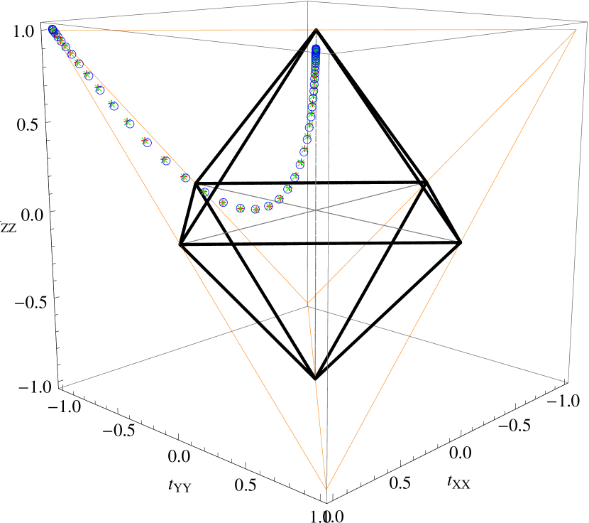
(a)

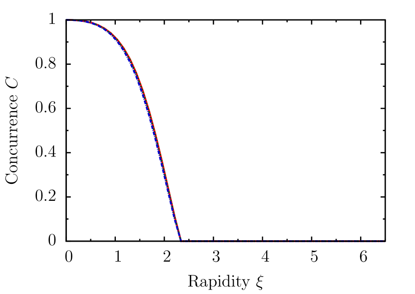
(b)

Figure 15: (Color online.) Spin (a) orbit and (b) concurrence for Gaussian momenta with $\sigma/m=1,2,4$. Product momenta are given by $f_{\times}$ with $\pm\mathbf{p}_{0}=\pm\mathbf{p}_{X0}$ and $\pm\mathbf{p}^{\perp}_{0}=\pm\mathbf{p}_{Y0}$. Data for $\sigma/m=1$ is shown with (a) the red “+” and (b) the red solid line, $\sigma/m=2$ with (a) the green “$\times$” and (b) the green dotted line, $\sigma/m=4$ with (a) the blue “$\bigcirc$” and (b) the blue dot-dashed line. (a) Initial state $\mathop{\left|\Phi_{+}\right\rangle}$ corresponds to vertex $(1,-1,1)$.

The orbits exhibit interesting behavior, initially showing a pattern that is analogous to the state $f_{\Sigma}$ for the case $R_{i}\otimes R_{j}$, see Fig. 8. However, after arriving the octahedron, we see different behavior: the orbit changes course and evolves towards the top of the upper pyramid. When the spins reach maximal rotation, the state becomes close to an equal mixture of projectors onto $\mathop{\left|\Phi_{+}\right\rangle}$ and $\mathop{\left|\Phi_{-}\right\rangle}$, never leaving the octahedron of separable states. This explains why concurrence vanishes for all $\xi>2.3$.

Let us next consider the correspondence between the $z$-axis centered momenta and the $f_{\times}$ model. When analyzing the curious behavior of the $z$-axis Gaussians in the previous section, we resorted to a naive 2D model in the $xz$-plane. Realistic Gaussians however involve a third dimension as well, and generalizing the 2D model to three dimensions naturally leads to the state which is given by $f_{\times}$. This explains why there is a close match between the orbits of the $z$-axis centered states with the large momenta $(0,0,-98.5)$ and those of $f_{\times}$ above. This raises the question of whether the $z$-axis centered states shown in Fig. 11 can be modeled using the $f_{\times}$ states with suitably chosen momenta. Proceeding in the same naive way as for the 2D model, let us approximate the states in Fig. 11 using $f_{\times}$ and assuming that the momenta are described by

$$\pm\mathbf{p}_{0}=\pm\mathbf{q}_{0}=(0,\pm 3,p_{z}),\quad\pm\mathbf{p}^{\perp}_{0}=\pm\mathbf{q}^{\perp}_{0}=(\pm 3,0,p_{z}),$$

where $p_{z}$ takes the values $-4$, $0$ and $4$. We plot the orbits and concurrence for $\sigma/m=0.25$ in Fig. 16, where we have chosen $\sigma$ to be smaller than above in order to minimize width related effects.

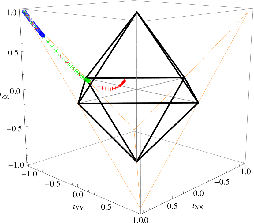
(a)

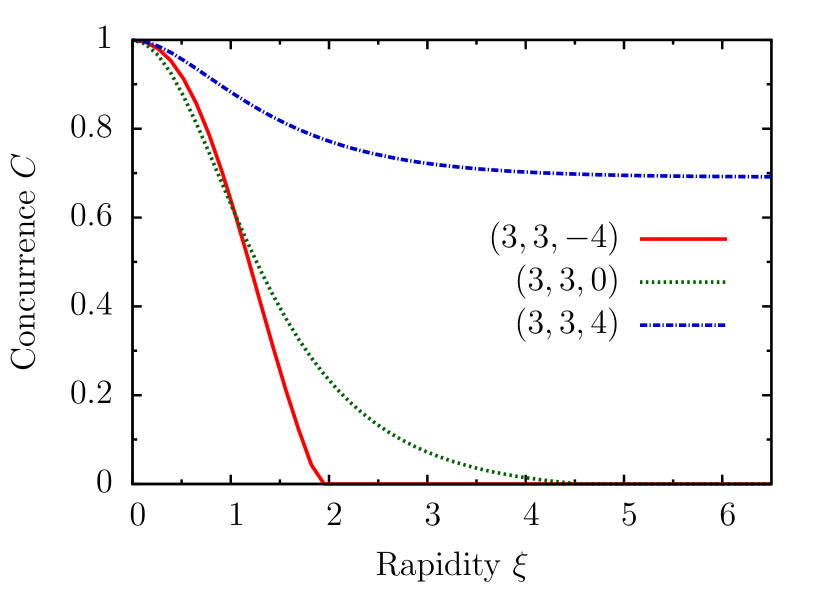
(b)

Figure 16: (Color online.) Spin (a) orbit and (b) concurrence for Gaussian momenta with $\sigma/m=0.25$. Product momenta are given by $f_{\times}$. Data for $(3,3,-4)$ is shown with (a) the red “+” and (b) the red solid line, $(3,3,0)$ with (a) the green “$\times$” and (b) the green dotted line, $(3,3,4)$ with (a) the blue “$\bigcirc$” and (b) the blue dot-dashed line. (a) Initial state $\mathop{\left|\Phi_{+}\right\rangle}$ corresponds to vertex $(1,-1,1)$.

While the agreement with Fig. 11 is not perfect, one can easily recognize the features present in the original $z$-axis case. The concurrence of the $f_{\times}$ model exhibits roughly the same kind of dependence on the boost angle as the $z$-axis centered states. Although the momenta with $p_{z}=4$ diverge considerably from those with $(0,0,4)$ in Fig. 11, the fit is relatively good for $p_{z}=-4$ and $p_{z}=0$ considering this is a simple model. The orbits follow the same pattern, with the one for $p_{z}=4$ deviating more, and those for $p_{z}=0$ and $p_{z}=-4$ relatively little from the $z$-axis centered states.

To summarize, all along we have been using the notion that systems involving continuous momenta, and specifically those of Gaussian form, can be understood in terms of discrete models, possibly containing many momentum eigenstates. The foregoing discussion bolsters this claim by showing that in some cases Gaussian momenta admit very simple models. In particular the momenta centered at the axis parallel to the direction of boost can be modeled by sampling four narrow Gaussians.

XIII Correspondence to discrete systems

We would like to comment on the relation between continuous and discrete systems which is implicit in all the cases discussed above: when the width of the Gaussian becomes small enough, we observe a good match with discrete systems. In many cases, the behavior of the latter can be calculated analytically Palge and Dunningham (2015).

By way of example, consider rotations of type $R_{i}\otimes R_{i}$ generated by product momenta $f_{\Sigma}$. Comparison with the plots of the discrete model, see Fig. 5 in Palge and Dunningham (2015), shows that for $\sigma/m=1$ the behavior of the continuous and the discrete model coincide to quite a high degree of accuracy. The orbit of the continuous system follows the same path as the discrete one, almost reaching the rest frame state $\mathop{\left|\Phi_{+}\right\rangle}$. The reason it stops short of $\mathop{\left|\Phi_{+}\right\rangle}$ is that while in the discrete model we assume that the system reaches the maximum TWR of $180^{\circ}$, the maximum rotation implemented by the continuous model at $\xi=6.5$ is $\omega_{m}\approx 163^{\circ}$ or $2.81\;\text{rad}$. Substituting $\omega_{m}$ into the expression that describes the discrete orbit, Eq. (63) in Palge and Dunningham (2015), yields $t_{Y\otimes Y}(\omega_{m})=(0.9,-1,0.9)$, which is in good agreement with the numerically calculated value $(0.89,-0.99,0.90)$ representing the final state for $\sigma/m=1$ in Fig. 7(a). Likewise, the concurrence of the discrete model, Eq. (62) with $\lambda=1$ in Palge and Dunningham (2015), evaluates to $C(\omega_{m})=0.89$, showing again good fit with the continuous model.

This pattern is generic in that a similar analysis can be run for each type of rotation. Although it might seem that the case $R_{i}\otimes\mathbb{1}$ in section X.1 provides a counterexample, this is not true. The reason it deviates from the discrete behavior is that the identity map can not be implemented accurately enough. Realistic systems that are characterized by wave packets of finite width always contain momenta which induce some rotation on the spin field, thereby diverging from idealized behavior.

XIV Discussion and summary

In this paper we have studied spin entanglement of two particles with continuous momenta. We have surveyed a number of boost scenarios involving momenta in product states. Attention was confined to pure spins, which were assumed to be in the maximally entangled Bell state $\mathop{\left|\Phi_{+}\right\rangle}$.

Our results confirm the general conclusion that Lorentz boosts cause non-trivial behavior of spin entanglement of a two particle system. The details of the behavior, however, are strongly determined by the boost situation at hand, that is, the momentum state and geometry involved. While there are states and geometries that leave entanglement invariant, most scenarios we have studied lead to significant changes of concurrence. An example of the former was given by the product momenta $f_{\mathrm{EPRB}}$ with $\sigma/m=1$ in the EPRB situation which leaves the entanglement of the Bell state invariant. The rest of the momenta causes changes of spin entanglement between the maximal value and zero.

Although the analysis was numerical throughout, the lack of analytic models was to some extent compensated by modeling continuous momenta in terms of discrete ones. In this picture, systems involving continuous momenta can be thought of as fields comprising spins at a large number of discrete momenta, where boosting means that each spin undergoes a different, momentum dependent rotation for a given value of rapidity. The difference between the behaviors of the EPRB momenta and the rest of the systems can then be explained in terms of the rotations that the discrete models generate on the spin degree of freedom.

It is also worthwhile highlighting the different roles that momentum states and geometries play in a boost scenario. Fixing a momentum state is equivalent to choosing a particular class of spin orbits from the set of all possible orbits. The boost geometry, on the other hand, gives a handle that enables one to tune the magnitude of the rotation that the spins are subjected to. In other words, specifying a geometry means picking a particular spin orbit from the class of spin orbits associated with a certain momentum state. As an illustration, consider Fig. 16 which shows the same momentum state $f_{\times}$ with three different boost angles. By specifying that the momenta are given by $f_{\times}$ we determine that the spin orbit is the one associated with the momentum $f_{\times}$ as opposed to, for instance, $f_{\Sigma}$. Further, by fixing the boost angle one determines the upper bound of the TWR for spins, thereby choosing a particular orbit from the class associated with $f_{\times}$. The reason for choosing extremely large momenta and large boost angles was that we wanted to obtain the longest orbit in the particular class. Scenarios with smaller boost angles are subsumed in the sense that they are given by shorter orbits in the same class: orbits whose endpoint corresponds to a smaller maximum TWR.

We would also like to comment on the role of the initial states. While we assumed from the start that the focus is exclusively on systems whose spin and momentum degrees of freedom factorize, the spin–momentum entangled states have been, to some extent, implicit in the investigation too. This is because all inertial frames are equivalent and Lorentz boosts are group elements, meaning that we are guaranteed to have inverse elements and the scenarios can be read in the reverse direction. One can regard the final state, which typically contains spin–momentum entanglement, as the rest frame state, and take the inverse boost to obtain the initial state. For instance, consider the boosted state $\frac{1}{4}\mathbb{1}_{4}$ at $\xi=2.2$, which is represented by $(0,0,0)$ in Fig. 8. Applying the inverse boost gives back the original maximally entangled Bell state $\mathop{\left|\Phi_{+}\right\rangle}$. All plots can be interpreted this way.

This points to an important asymmetry between spin–momentum product versus entangled states. Whereas the latter can lead to an increase of spin–spin entanglement, it has been shown that the former can never cause such behavior Gingrich and Adami (2002).

Finally, we would like to emphasize the usefulness of visualization of spin orbits, which provided further insight into the behavior of entanglement. We gained a more detailed understanding of how varying the initial states, their widths and momenta, changed the spin concurrence. The hope is that the results obtained in this paper contribute to a better understanding of entanglement in relativity and could lead to future applications which might be of interest in relativistic quantum information.

XV Acknowledgments

Veiko Palge was supported by EU through the ERDF CoE program grant TK133 and by the Estonian Research Council via IUT2-27. Stefan Groote and Hannes Liivat were supported by the Estonian Research Council via IUT2-27. We would like to thank Hardi Veermäe for a number of helpful suggestions.

Appendix A particles in the Wigner representation

A.1 Conventions

We will use natural units where $\hbar=c=1$. Spacetime metric is $\mathrm{diag}(+---)$. Latin indices $i,j,k$ etc. take values in three tuples $(x,y,z)$ or $(1,2,3)$ while Greek indices $\mu,\nu$ etc. run over $(t,x,y,z)$ or $(0,1,2,3)$. Three vectors use boldface whereas four vectors are given in ordinary type. For instance, the four momentum is $p^{\mu}=(p^{0},\mathbf{p})$ with the norm $p^{\mu}p_{\mu}=(p^{0})^{2}-\mathbf{p}^{2}=m^{2}$.

A.2 Particles

In this section, we summarize the background for the relativistic quantum mechanical constructions used in the paper. Throughout we work in the Wigner representation which can be found in references Bogolubov et al. (1975); Sexl and Urbantke (2001). The single particle states are given by a unitary irreducible representation of the Poincaré group where a representation is labelled by mass $m>0$ and the intrinsic spin $s$ which takes integral or half-integral values. The representation can be realized in the space $\bigoplus^{2s+1}L^{2}(\Gamma^{+}_{m})$ of square integrable functions on the forward mass hyperboloid $\Gamma^{+}_{m}=\{p\in\mathbf{M}:p^{2}=m^{2},p^{0}>0\}$ where the scalar product is defined as

$$\langle\phi|\psi\rangle=\sum_{\sigma}\int\mathrm{d}\mu(p)\,\phi^{*}_{\sigma}(p)\psi_{\sigma}(p),$$ (53)

with $\mathrm{d}\mu(p)=[2E(\mathbf{p})]^{-1}\mathrm{d}^{3}\mathbf{p}$ being the Lorentz invariant integration measure. In this paper we specialize on spin-$1/2$ systems, then the state space is given by

$$\mathcal{H}=L^{2}(\mathbb{R}^{3})\oplus L^{2}(\mathbb{R}^{3})=L^{2}(\mathbb{R}^{3},\mathbb{C}^{2})=L^{2}(\mathbb{R}^{3})\otimes\mathbb{C}^{2}.$$ (54)

In order to define basis vectors, we start by specifying the rest frame states in terms of four momentum $P^{\mu}$, square of total angular momentum $\mathbf{J}^{2}$ and the $z$-component of angular momentum $J_{z}$,

$$P^{\mu}\mathop{\left|\mathbf{0},\lambda\right\rangle} =p^{\mu}_{0}\mathop{\left|\mathbf{0},\lambda\right\rangle},$$

$$\mathbf{J}^{2}\mathop{\left|\mathbf{0},\lambda\right\rangle} =s(s+1)\mathop{\left|\mathbf{0},\lambda\right\rangle},$$ (55)

$$J_{z}\mathop{\left|\mathbf{0},\lambda\right\rangle} =\lambda\mathop{\left|\mathbf{0},\lambda\right\rangle},$$

where $\mathbf{0}$ denotes $\mathbf{p}=0$ with $p^{\mu}_{0}=(m,\mathbf{0})$, and we have abbreviated $\mathop{\left|\mathbf{p},\lambda\right\rangle}=\mathop{\left|\mathbf{p}\right\rangle}\otimes\mathop{\left|\lambda\right\rangle}$. Because the particle is at rest, $s$ and $\lambda$ refer to the spin and the $z$-component of the particle. We next generate a complete basis, which consists of the general eigenvectors of $P^{\mu}$, by acting on the rest frame state with a pure, rotation free Lorentz boost,

$$\mathop{\left|\mathbf{p},\lambda\right\rangle}=U[L(\mathbf{p})]\mathop{\left|\mathbf{0},\lambda\right\rangle},$$ (56)

where $U[L(\mathbf{p})]$ is a unitary representation of boost $L(\mathbf{p})$ that takes the rest momentum $(m,\mathbf{0})=p_{0}$ to an arbitrary momentum,

$$L(\mathbf{p})\,(m,\mathbf{0})=(E(\mathbf{p}),\mathbf{p}),$$ (57)

with $E(\mathbf{p})=\sqrt{\mathbf{p}^{2}+m^{2}}$. The basis vectors $\mathop{\left|\mathbf{p},\lambda\right\rangle}$ span the single particle state space $\mathcal{H}$ and we can write a generic state as

$$\mathop{\left|\Psi\right\rangle}=\sum_{\sigma}\int\mathrm{d}\mu(p)\,\psi_{\sigma}(\mathbf{p})\mathop{\left|\mathbf{p},\sigma\right\rangle},$$ (58)

The basis states are normalized as follows,

$$\langle\mathbf{p}^{\prime},\sigma^{\prime}|\mathbf{p},\sigma\rangle=2E(\mathbf{p})\delta^{3}(\mathbf{p}-\mathbf{p}^{\prime})\delta_{\sigma\sigma^{\prime}}.$$ (59)

The action of a generic Lorentz transformation $\Lambda$ on an element of basis is given by

$$U(\Lambda)\mathop{\left|\mathbf{p},\sigma\right\rangle}=\sum_{\lambda}\mathop{\left|\Lambda\mathbf{p},\lambda\right\rangle}D_{\lambda\sigma}[W(\Lambda,\mathbf{p})],$$ (60)

where $W(\Lambda,\mathbf{p})$ is the Wigner rotation

$$W(\Lambda,\mathbf{p})\equiv L^{-1}(\Lambda\mathbf{p})\Lambda L(\mathbf{p})$$ (61)

that leaves $p_{0}$ invariant, $p_{0}=Wp_{0}$. For massive particles, $W\in\mathrm{SO}(3)$ is a rotation and $D[W(\Lambda,\mathbf{p})]$ is its representation. For spin-$1/2$ particles, the latter is an element of $\mathrm{SU}(2)$, whose concrete form in terms of momenta and rapidities can be found in Halpern (1968).

A.3 Lorentz transformations on particles

One can now calculate the transformation on the wave function. In the Lorentz boosted frame, the state is $\mathop{\left|\Psi^{\Lambda}\right\rangle}=U(\Lambda)\mathop{\left|\Psi\right\rangle}$, so we have

$$\mathop{\left|\Psi^{\Lambda}\right\rangle} =\sum_{\sigma}\int\mathrm{d}\mu(p)\,\psi_{\sigma}(\mathbf{p})\sum_{\lambda}\mathop{\left|\Lambda\mathbf{p},\lambda\right\rangle}D_{\lambda\sigma}[W(\Lambda,\mathbf{p})]$$

$$=\sum_{\lambda}\int\mathrm{d}\mu(p^{\prime})\,\sum_{\sigma}D_{\lambda\sigma}[W(\Lambda,\Lambda^{-1}\mathbf{p}^{\prime})]\psi_{\sigma}(\Lambda^{-1}\mathbf{p}^{\prime})\mathop{\left|\mathbf{p}^{\prime},\lambda\right\rangle}$$

$$=\sum_{\lambda}\int\mathrm{d}\mu(p)\,\psi^{\Lambda}_{\lambda}(\mathbf{p})\mathop{\left|\mathbf{p},\lambda\right\rangle},$$ (62)

where $\mathbf{p}^{\prime}=\Lambda\mathbf{p}$ and we used the fact that the integration measure is Lorentz covariant, $\mathrm{d}\mu(p)=\mathrm{d}\mu(\Lambda p)$, with a relabelling of dummy variables in the last line, $\mathbf{p}^{\prime}\rightarrow\mathbf{p}$. Hence we have,

$$\psi^{\Lambda}_{\lambda}(\mathbf{p})=\sum_{\sigma}D_{\lambda\sigma}[W(\Lambda,\Lambda^{-1}\mathbf{p})]\psi_{\sigma}(\Lambda^{-1}\mathbf{p}).$$ (63)

The state of a two particle system belongs to $\mathcal{H}_{2}=\mathcal{H}_{1}\otimes\mathcal{H}_{1}$ where $\mathcal{H}_{1}$ is the one particle Hilbert space described above. A Lorentz boost $\Lambda$ acts on the two particle state by $U(\Lambda)\otimes U(\Lambda)$ and in analogy to the single particle case we calculate that the corresponding transformation of the wave function is given by

$$\psi^{\Lambda}_{\lambda\kappa}(\mathbf{p},\mathbf{q}) =\sum_{\sigma,\xi}D_{\lambda\sigma}\!\left[W(\Lambda,\Lambda^{-1}\mathbf{p})\right]D_{\kappa\xi}\!\left[W(\Lambda,\Lambda^{-1}\mathbf{q})\right]$$

$$\phantom{AAAAAAAAA}\times\psi_{\sigma\xi}(\Lambda^{-1}\mathbf{p},\Lambda^{-1}\mathbf{q}).$$ (64)

References

- Czachor (1997) M. Czachor, Physical Review A 55, 72 (1997).
- Gingrich and Adami (2002) R. M. Gingrich and C. Adami, Physical Review Letters 89, 270402 (2002).
- Peres et al. (2002) A. Peres, P. F. Scudo, and D. R. Terno, Physical Review Letters 88, 230402 (2002).
- Alsing and Milburn (2002) P. M. Alsing and G. J. Milburn, Quantum Information and Computation 2, 487 (2002).
- Ahn et al. (2002) D. Ahn, H.-J. Lee, and S. W. Hwang, arXiv:quant-ph/0207018 (2002).
- Ahn et al. (2003a) D. Ahn, H.-J. Lee, Y. H. Moon, and S. W. Hwang, Physical Review A 67, 012103 (2003a).
- Ahn et al. (2003b) D. Ahn, H.-J. Lee, and S. W. Hwang, Physical Review A 67, 032309 (2003b).
- Czachor and Wilczewski (2003) M. Czachor and M. Wilczewski, Physical Review A 68, 010302 (2003).
- Moon et al. (2004) Y. H. Moon, S. W. Hwang, and D. Ahn, Progress of Theoretical Physics 112, 219 (2004).
- Lee and Chang-Young (2004) D. Lee and E. Chang-Young, New Journal of Physics 6, 67 (2004).
- Czachor (2005) M. Czachor, Physical Review Letters 94, 078901 (2005).
- Lamata et al. (2006) L. Lamata, M. A. Martin-Delgado, and E. Solano, Physical Review Letters 97, 250502 (2006).
- Alsing et al. (2006) P. M. Alsing, I. Fuentes-Schuller, R. B. Mann, and T. E. Tessier, Physical Review A 74, 032326 (2006).
- Chakrabarti (2009) A. Chakrabarti, Journal of Physics A: Mathematical and Theoretical 42, 245205 (2009).
- Fuentes et al. (2010) I. Fuentes, R. B. Mann, E. Martín-Martínez, and S. Moradi, Physical Review D 82, 045030 (2010).
- Friis et al. (2010) N. Friis, R. A. Bertlmann, and M. Huber, Physical Review A 81, 042114 (2010).
- Palge and Dunningham (2012) V. Palge and J. Dunningham, Physical Review A 85, 042322 (2012).
- Alsing and Fuentes (2012) P. M. Alsing and I. Fuentes, Classical and Quantum Gravity 29, 224001 (2012).
- Terashima and Ueda (2003) H. Terashima and M. Ueda, International Journal of Quantum Information 01, 93 (2003).
- Caban and Rembieliński (2005) P. Caban and J. Rembieliński, Physical Review A 72, 012103 (2005).
- Caban and Rembieliński (2006) P. Caban and J. Rembieliński, Physical Review A 74, 042103 (2006).
- Jordan et al. (2006) T. Jordan, A. Shaji, and E. Sudarshan, Physical Review A 73, 032104 (2006).
- Jordan et al. (2007) T. Jordan, A. Shaji, and E. Sudarshan, Physical Review A 75, 022101 (2007).
- Palge et al. (2011) V. Palge, V. Vedral, and J. A. Dunningham, Physical Review A 84, 044303 (2011).
- Note (1) A related study that involves systems with discrete momenta along with an extension to mixed spin states can be found in Palge and Dunningham (2015).
- Note (2) The unitary irreducible representation is due to Wigner Wigner (1939). A standard treatment of the two representations is given by Bogolubov et al. (1975). See Polyzou et al. (2012) for a very readable account on the relationship between the two frameworks and Caban et al. (2013) for a discussion in the context of spin observable in the Dirac theory.
- Caban et al. (2013) P. Caban, J. Rembieliński, and M. Włodarczyk, Physical Review A 88, 022119 (2013).
- Note (3) We will use the abbreviation TWR in honor of Thomas’s contribution of discovering the Thomas precession Thomas (1926, 1927).
- Note (4) With the caveat that strictly considered the momentum state is not a qubit, so we call it a momentum system.
- Note (5) Entangled momenta are discussed in a related paper.
- Palge and Dunningham (2015) V. Palge and J. Dunningham, Annals of Physics 363, 275 (2015).
- Sexl and Urbantke (2001) R. U. Sexl and H. K. Urbantke, Relativity, Groups, Particles: Special Relativity and Relativistic Symmetry in Field and Particle Physics, rev. ed. ed. (Springer, New York, 2001).
- Bogolubov et al. (1975) N. N. Bogolubov, A. A. Logunov, and I. T. Todorov, Introduction to Axiomatic Quantum Field Theory (W.A.Benjamin, 1975).
- MacFarlane (1963) A. J. MacFarlane, Journal of Mathematical Physics 4, 490 (1963).
- Wootters (1998) W. Wootters, Physical Review Letters 80, 2245 (1998).
- Rhodes and Semon (2004) J. A. Rhodes and M. D. Semon, Am. J. Phys. 72, 943 (2004).
- Halpern (1968) F. R. Halpern, Special Relativity and Quantum Mechanics (Prentice-Hall, 1968).
- Einstein et al. (1935) A. Einstein, B. Podolsky, and N. Rosen, Physical Review 47, 777 (1935).
- Bohm (1951) D. Bohm, Quantum Theory, Prentice-Hall physics series (Prentice-Hall, New York, 1951).
- Note (6) From a more general perspective, it is interesting to consider mixed states as well. See Palge and Dunningham (2015) for an extension to the Werner states.
- Bengtsson and Życzkowski (2006) I. Bengtsson and K. Życzkowski, Geometry of Quantum States: An Introduction to Quantum Entanglement (Cambridge University Press, 2006).
- Bertlmann et al. (2002) R. A. Bertlmann, H. Narnhofer, and W. Thirring, Physical Review A 66, 032319 (2002).
- Wigner (1939) E. Wigner, Annals of Mathematics Second Series, 40, 149 (1939).
- Polyzou et al. (2012) W. N. Polyzou, W. Glöckle, and H. Witała, Few-Body Systems 54, 1667 (2012).
- Thomas (1926) L. H. Thomas, Nature 117, 514 (1926).
- Thomas (1927) L. H. Thomas, Philosophical Magazine 7, 3, 1 (1927).