Multi-terminal Anderson impurity model in nonequilibrium: Analytical perturbative treatment

Abstract

We study the nonequilibrium spectral function of the single-impurity Anderson model connecting with multi-terminal leads. The full dependence on frequency and bias voltage of the nonequilibrium self-energy and spectral function is obtained analytically up to the second-order perturbation regarding the interaction strength $U$. High and low bias voltage properties are analyzed for a generic multi-terminal dot, showing a crossover from the Kondo resonance to the Coulomb peaks with increasing bias voltage. For a dot where the particle-hole symmetry is not present, we construct a current-preserving evaluation of the nonequilibrium spectral function for arbitrary bias voltage. It is shown that finite bias voltage does not split the Kondo resonance in this order, and no specific structure due to multiple leads emerges. Overall bias dependence is quite similar to finite temperature effect for a dot with or without the particle-hole symmetry.

I Introduction

Understanding strong correlation effect away from equilibrium has been one of the most interesting yet challenging problems in condensed matter physics. A prominent realization of such phenomena is embodied in quantum transport through a nanostructure under finite bias voltage. To understand the interplay of the correlation effect and nonequilibrium nature, nonequilibrium version of the single impurity Anderson model (SIAM) and its extensions have been serving and continue to do so as a central theoretical model. The SIAM is indeed considered to be one of the best studied strongly correlated model, and despite its apparent simplicity, it exhibits rich physics already in equilibrium, such as the Coulomb blockade and the Kondo physics that have been observed in experiments. Equilibrium properties of the SIAM have been well understood thanks to concerted efforts of several theoretical approaches over years — by perturbative treatment, Fermi liquid description, as well as exact results by the Bethe ansatz method and numerical renormalization group (NRG) calculations (see for instance, Tsvelick and Wiegmann, 1983a; Hewson, 1993; Bulla et al., 2008.) In contrast, the situation of the nonequilibrium SIAM is not so satisfactory. Each of the above approaches has met some difficulty in treating nonequilibrium phenomena. A theoretical approach that can deal with the strong correlation effect in nonequilibrium is still called for.

Notwithstanding, a number of analytical and numerical methods have been devised to investigate nonequilibrium stationary phenomena: nonequilibrium perturbation approaches Hershfield et al. (1992); Fujii and Ueda (2003, 2005); Hamasaki (2007); Mühlbacher et al. (2011) and its modifications Yeyati et al. (1993, 1999); Aligia (2006), the non-crossing approximation Meir et al. (1993), the functional renormalization group treatment Schmidt and Wölfle (2010), quantum Monte Carlo calculations on the Keldysh contour Schmidt et al. (2008); Werner et al. (2010), the iterative real-time path integral method Weiss et al. (2008) and so on. Unfortunately those approaches fail to give a consistent picture concerning the finite bias effect on the dot spectral function, particularly regarding a possible splitting of the Kondo resonance.

As for the equilibrium SIAM, the second-order perturbation regarding the Coulomb interaction $U$ on the dot Yamada (1975a, b); Yoshida and Yamada (1975); Zlatić and Horvatić (1983) is known to capture essential features of Kondo physics and agrees qualitatively well with exact results obtained by the Bethe ansatz and NRG approaches Tsvelick and Wiegmann (1983a); Hewson (1993); Zlatić and Horvatić (1983). Such good agreement seems to persist in nonequilibrium stationary state at finite bias voltage. For the two-terminal particle-hole (PH) symmetric SIAM, a recent study by Mühlbacher et al. (2011) showed that the nonequilibrium second order perturbation calculation of the spectral function agrees with that calculated by the diagrammatic quantum Monte Carlo simulation, excellently up to interaction strength $U\sim 2\gamma$ (where $\gamma$ is the total relaxation rate due to leads); pretty well even for $U\lesssim 8\gamma$ at bias voltage $eV\lesssim 2\gamma$. A typical magnitude of $U/\gamma$ of a semiconductor quantum dot is roughly $1\sim 10$ depending on the size and the configuration of the dot. Therefore, there is a good chance of describing a realistic system within the validity of nonequilibrium perturbation approach.

The great advantage of semiconductor dot systems is to allow us to control several physical parameters. Those include changing gate voltage as well as configuring a more involved structure such as a multi-terminal dot Sun and Guo (2001); Lebanon and Schiller (2001); Cho et al. (2003); Sánchez and López (2005); Shah and Rosch (2006); Leturcq et al. (2005) or an interferometer embedding a quantum dot. Theoretical treatments often limit themselves to a system with the PH symmetry where the dot occupation number is fixed to be one half per spin. Although assuming the PH symmetry makes sense and comes in handy in extracting the essence of the Kondo resonance, we should bear in mind that such symmetry is not intrinsic and can be broken easily in realistic systems, by gate voltage, asymmetry of the coupling with the leads, or asymmetric drops of bias voltage Aligia (2012); Muñoz et al. (2013). The PH asymmetry commonly appears in a multi-terminal dot or in an interferometer embedding a quantum dot. It is also argued that the effect of the PH asymmetry might be responsible for the deviation observed in nonequilibrium transport experiments from the “universal” behavior of the PH symmetric SIAM Aligia (2012); Muñoz et al. (2013). To work on realistic systems, it is imperative to understand how the PH asymmetry affects nonequilibrium transport.

In this paper, we examine the second-order nonequilibrium perturbation regarding the Coulomb interaction $U$ of the multi-terminal SIAM. The PH symmetry is not assumed, and miscellaneous types of asymmetry of couplings to the leads and/or voltage drops are incorporated as a generic multi-terminal configuration. Our main focus is to provide solid analytical results of the behavior of the nonequilibrium self-energy and hence the dot spectral function for the full range of frequency and bias voltage, within the validity of the second-order perturbation theory of $U$. The result encompasses Fermi liquid behavior as well as incoherent non-Fermi liquid contribution, showing analytically that increasing finite bias voltage leads to a crossover from the Kondo resonance to the Coulomb blockade behaviors. The present work contrasts preceding perturbative studies Hershfield et al. (1992); Hamasaki (2004, 2007); Fujii and Ueda (2003, 2005) whose evaluations relied on either numerical means or a small-parameter expansion of bias voltage and frequency. The only notable exception, to the author’s knowledge, is a recent work by Mühlbacher et al. (2011), which succeeded in evaluating analytically the second-order self-energy for the two-terminal PH symmetric dot. Intending to apply such analysis to a wider range of realistic systems and examine the effect that the two-terminal PH symmetric SIAM cannot capture, we extend their approach to a generic multi-terminal dot where the PH symmetry may not necessarily be present.

An embarrassing drawback of using the nonequilibrium perturbation theory is that when one has it naively apply to the PH asymmetric SIAM, it may disrespect the preservation of the steady current. Hershfield et al. (1992) As a result, one then needs some current-preserving prescription, and different self-consistent schemes have been proposed and adopted. Yeyati et al. (1993); Matsumoto (2000); Aligia (2006) As will be seen, the current preserving condition involves all the frequency range, not only of low frequency region that validates Fermi liquid description but also of the incoherent non-Fermi liquid part (See Eq. (6) below). Therefore, an approximation based on the low energy physics, particularly the Fermi liquid picture, should be used with care. The self-energy we will construct analytically is checked to satisfy the spectral sum rule at finite bias voltage, so that we regard it as giving a consistent description for the full range of frequency in nonequilibrium. By taking its advantage, we also demonstrate a self-consistent, current-preserving calculation of the nonequilibrium spectral function for a system where the PH symmetry is not present.

The paper is organized as follows. In Sec. II, we introduce the multi-terminal SIAM in nonequilibrium. We review briefly how to obtain the exact current formula by clarifying the role of the current conservation at finite bias voltage. Section III presents analytical expression of the retarded self-energy for a general multi-terminal dot up to the second-order of the interaction strength. Subsequently in Sec. IV, we examine and discuss its various analytical behaviors including high- and low-bias voltage limits. Sec. V is devoted to constructing a non-equilibrium spectral function using the self-energy obtained in the previous section. We focus our attention on two particular situations: (1) self-consistent, current-preserving evaluation of the nonequilibrium spectral function for the two-terminal PH asymmetric SIAM, and (2) multi-terminal effect of the PH symmetric SIAM. Finally we conclude in Sec. VI. Mathematical details leading to our main analytical result Eq. (21) as well as other necessary material regarding dilogarithm is summarized in Appendices.

II The multi-terminal Anderson impurity model and the current formula

II.1 Model

The model we consider is the single impurity Anderson model connecting with multiple leads $a=1,\ldots,N$ whose chemical potentials are sustained by $\mu_{a}$. The total Hamiltonian of the system consists of $H=H_{D}+H_{T}+\sum_{a}H_{a}$, where $H_{D}$, $H_{T}$ and $H_{a}$ represent the dot Hamiltonian with the Coulomb interaction, the hopping term between the dot and the leads, and the Hamiltonian of a noninteracting lead $a$, respectively. They are specified by

$$H_{D}=\sum_{\sigma}\epsilon_{d}\,n_{\sigma}+Un_{\uparrow}n_{\downarrow},$$ (1)

$$H_{T}=\sum_{a,\sigma}\left(V_{da}\,d^{\dagger}_{\sigma}c_{a\boldsymbol{k}\sigma}+V_{ad}\,c^{\dagger}_{a\boldsymbol{k}\sigma}d_{\sigma}\right),$$ (2)

where $n_{\sigma}=d^{\dagger}_{\sigma}d_{\sigma}$ is the dot electron number operator with spin $\sigma$ and $c_{a\boldsymbol{k}\sigma}$ are electron operators at the lead $a$. In the following, we consider the spin-independent transport case, but an extension to the spin-dependence situation such as in the presence of magnetic field or ferromagnetic leads is straightforward. When applying the wide-band limit, all the effect of the lead $a$ is encoded in terms of its chemical potential $\mu_{a}$ and relaxation rate $\gamma_{a}=\pi|V_{da}|^{2}\rho_{a}$, where $\rho_{a}$ is the density of states of the lead $a$. The dot level $\epsilon_{d}$ controls the average occupation number on the dot; it corresponds roughly to $2$, $1$, $0$ for $\epsilon_{d}\lesssim-U$, $-U\lesssim\epsilon_{d}\lesssim 0$, and $0\lesssim\epsilon_{d}$, respectively. The PH symmetry is realized when $\epsilon_{d}=-U/2$ and $\langle n_{\sigma}\rangle=1/2$ (see Eqs. (6) and (13) below).

II.2 Multi-terminal current and current conservation

We here briefly summarize how the current through the dot is determined in a multi-terminal setting. Special attention is paid to the role of the current conservation because it has been known that nonequilibrium perturbation calculation does not respect it in general. Hershfield et al. (1992) We illustrate how to ensure the current conservation by requiring minimally. The argument below is valid regardless of a specific approximation scheme chosen, whether nonequilibrium perturbation or any other approach.

Following the standard protocol of the Keldysh formulation Meir and Wingreen (1992), we start with writing the current $I_{a}$ flowing from the lead $a$ to the dot in terms of the dot’s lesser Green function $G^{-+}_{\sigma}$ and the retarded one $G^{R}_{\sigma}$:

$$I_{a}=-\frac{e}{\pi\hbar}\sum_{\sigma}\int d\omega\left[i\gamma_{a}\,G^{-+}_{\sigma}(\omega)-2\gamma_{a}f_{a}\mathop{\mathrm{Im}}\nolimits G^{R}_{\sigma}(\omega)\,\right],$$ (3)

where $f_{a}(\omega)=1/(e^{\beta(\omega-\mu_{a})}+1)$ is the Fermi distribution function at the lead $a$. As the present model preserves the total spin as well as charge, the net spin current flowing to the dot should vanish in the steady state, which imposes the integral relation between $G^{-+}_{\sigma}$ and $G^{R}_{\sigma}$,

$$\int^{\infty}_{-\infty}d\omega\left[i\gamma\,G^{-+}_{\sigma}(\omega)+2\gamma\bar{f}(\omega)\mathop{\mathrm{Im}}\nolimits G^{R}_{\sigma}(\omega)\right]=0.$$ (4)

Here we have introduced the total relaxation rates $\gamma=\sum_{a}\gamma_{a}$ and the effective Fermi distribution $\bar{f}$ weighted by the leads,

$$\bar{f}(\omega)=\sum_{a}\frac{\gamma_{a}}{\gamma}\,f_{a}(\omega).$$ (5)

When we ignore the energy dependence of the relaxation rates $\gamma_{a}$, we can recast Eq. (4) into a more familiar form

$$n_{\sigma}=-\frac{1}{\pi}\int^{\infty}_{-\infty}d\omega\,\bar{f}(\omega)\mathop{\mathrm{Im}}\nolimits G^{R}_{\sigma}(\omega),$$ (6)

because $2i\pi n_{\sigma}=\int d\omega G^{-+}_{\sigma}(\omega)$ is the definition of the exact dot occupation number. Note the quantity $-\mathop{\mathrm{Im}}\nolimits G^{R}_{\sigma}(\omega)/\pi$ is nothing but the exact dot spectral function out of equilibrium. We emphasize that Eq. (4) (or equivalently Eq. (6)) is the minimum, exact requirement that ensures the current preservation. It constrains the exact $G^{-+}$ and $G^{R}$ that depend on the interaction as well as bias voltage in a nontrivial way. One can accordingly eliminate $\int d\omega\,G^{-+}(\omega)$ in $I_{a}$, to reach the Landauer-Buttiker type current formula at the lead $a$,

$$I_{a}=-\frac{e}{\pi\hbar}\sum_{b,\sigma}\frac{\gamma_{a}\gamma_{b}}{\gamma}\int d\omega\,(f_{b}-f_{a})\mathop{\mathrm{Im}}\nolimits G^{R}_{\sigma}(\omega).$$ (7)

Or, the current conservation allows us to write it as

$$I_{a}=\frac{e\gamma_{a}}{\hbar}\sum_{\sigma}\left[n_{\sigma}-\mathcal{N}_{\sigma}(\mu_{a})\right],$$ (8)

where $\mathcal{N}_{\sigma}(\varepsilon)$ is the exact number of states with spin $\sigma$ at finite temperature in general, defined by

$$\mathcal{N}_{\sigma}(\mu)=-\frac{1}{\pi}\int d\varepsilon\,\frac{\mathop{\mathrm{Im}}\nolimits G^{R}_{\sigma}(\varepsilon)}{e^{\beta(\varepsilon-\mu)}+1}.$$ (9)

It tells us that differential conductance $\partial I_{a}/\partial\mu_{a}$ with fixing all other $\mu$’s is proportional to the nonequilibrium dot spectral function, provided changing $\mu_{a}$ does not affect the occupation number Sun and Guo (2001); Lebanon and Schiller (2001); Cho et al. (2003); Sánchez and López (2005). Such situation is realized, for instance, when a probe lead couples weakly to the dot.

The case of a noninteracting dot always satisfies the current preserving condition Eq. (4) as $G^{-+}_{\sigma}(\omega)=-2i\bar{f}(\omega)\mathop{\mathrm{Im}}\nolimits G^{R}_{\sigma}(\omega)$ holds for any $\omega$; the distribution function of dot electrons $f_{\text{dot}}(\omega)=G^{-+}(\omega)/(2i\pi)$ is equal to $-\bar{f}(\omega)\mathop{\mathrm{Im}}\nolimits G^{R}_{\sigma}(\omega)/\pi$. This is not the case for an interacting dot, however. As for the interacting case, not so much can be said. We only see the special case with the two-terminal PH symmetric dot satisfy Eq. (6) by choosing $n_{\sigma}=1/2$ irrespective of interaction strength. Except for this PH symmetric case, a general connection between $G^{-+}$ and $G^{R}$ is not known so far. It is remarked that, based on the quasiparticle picture, a noninteracting relation $G^{-+}_{\sigma}(\omega)=-2i\bar{f}(\omega)\mathop{\mathrm{Im}}\nolimits G^{R}_{\sigma}(\omega)$ is sometimes used to deduce an approximate form of $G^{-+}$ out of $G^{R}$ for an interacting dot. Such approximation is called the Ng’s ansatz Ng (1993); Dinu et al. (2007). Although it might be be simple and handy, its validity is far from clear. We will not rely on such additional approximation below. It is also important to distinguish in Eq. (6) the electron occupation number $n_{\sigma}$ from the quasiparticle occupation number $\tilde{n}_{\sigma}$, as the two quantities are different at finite bias voltage since the Luttinger relation holds only in equilibrium Luttinger and Ward (1960). Contribution to the dot occupation number comes from all range of frequency, including the incoherent part. One sees fulfilling the spectral weight sum rule $-\int^{\infty}_{-\infty}d\omega\mathop{\mathrm{Im}}\nolimits G^{R}(\omega)/\pi=1$ crucial to have the dot occupation number $n_{\sigma}$ normalized correctly. In general, one needs to determine $n_{\sigma}$ appropriately to satisfy Eq. (6) as a function of interaction and chemical potentials of the leads. The applicability of quasi-particle approaches that ignores the incoherent part is unclear.

III Analytical evaluation of the self-energy

In this section, we evaluate analytically the nonequilibrium retarded self-energy up to the second order of interaction strength $U$ for the multi-terminal SIAM. We first examine the contribution at the first-order and the role of current preservation. Then we present the analytical result of the second-order self-energy in terms of dilogarithm.

Following the standard treatment of the Keldysh formulation, Lifshitz and Pitaevskii (1981) the nonequilibrium Green function and the self-energy take a matrix structure

$$\hat{G}=\begin{pmatrix}G^{--}&G^{-+}\\ G^{+-}&G^{++}\end{pmatrix};\quad\hat{\Sigma}=\begin{pmatrix}\Sigma^{--}&\Sigma^{-+}\\ \Sigma^{+-}&\Sigma^{++}\end{pmatrix},$$ (10)

satisfying symmetry relations $G^{--}+G^{++}=G^{-+}+G^{+-}$ and $\Sigma^{--}+\Sigma^{++}=-\Sigma^{-+}-\Sigma^{+-}$. The retarded Green function is defined by $G^{R}=G^{--}+G^{-+}$; the retarded self-energy, by $\Sigma^{R}=\Sigma^{--}+\Sigma^{-+}$.

To proceed evaluation, it is convenient to classify self-energy diagrams into the two types: the Hartree-type diagram (Fig. 1) that can be disconnected by cutting a single interaction line, and the rest which we call the correlation part and reassign the symbol $\Sigma$ to. The latter starts at the second-order. The resulting Green function (matrix) takes a form of

$$\hat{G}_{\sigma}(\omega)=\left[\hat{G}_{0\sigma}^{-1}(\omega)-U\tau_{3}\,n_{\bar{\sigma}}-\hat{\Sigma}_{\sigma}(\omega)\right]^{-1},$$ (11)

where $\tau_{3}$ represents a Pauli matrix of the Keldysh structure, and $n_{\bar{\sigma}}$ refers to the exact occupation number of the dot electron with the opposite spin. Accordingly, the corresponding retarded Green function becomes

$$G^{R}_{\sigma}(\omega)=\frac{1}{\omega-E_{d\sigma}+i\gamma-\Sigma_{\sigma}^{R}(\omega)},$$ (12)

where $E_{d\sigma}=\epsilon_{d}+Un_{\bar{\sigma}}$ is the Hartree level of the dot.

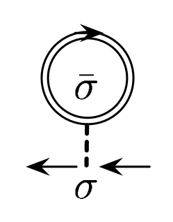
Figure 1: The Hartree-type contribution of the self-energy $U\tau_{3}\,n_{\bar{\sigma}}=\pm Un_{\bar{\sigma}}$. The double line refers to the exact Green function.

III.1 Current preservation at the first order

Before starting evaluating the correlation part $\Sigma^{R}$ that starts contributing at the second order, it is worthwhile to examine the current preserving condition Eq. (6) at the first order. At this order, it reduces to the self-consistent Hartree-Fock equation for the dot occupation number $n_{\sigma}^{0}$:

$$n_{\sigma}^{0}=\frac{1}{2}+\frac{1}{\pi}\sum_{a}\frac{\gamma_{a}}{\gamma}\arctan\left[\frac{\mu_{a}-\epsilon_{d}-Un_{\bar{\sigma}}^{0}}{\gamma}\right].$$ (13)

It shows how the two-terminal PH symmetric SIAM is special by choosing $\epsilon_{d}+U/2=0$, $\gamma_{a}=\gamma/2$ and $\mu_{a}=\pm eV/2$; the second term of the right-hand side vanishes by having the solution $n^{0}_{\sigma}=1/2$ even at finite bias voltage. It also indicates that the current preservation necessarily has the occupation number depend on asymmetry of the lead couplings as well as interaction strength for the PH asymmetric SIAM. Indeed, for a small deviation from the PH symmetry and bias voltage, we see the Hartree-Fock occupation number behave as

$$n_{\sigma}^{0}-\frac{1}{2}\approx\frac{\bar{\mu}-\epsilon_{d}-U/2}{\pi\gamma}\left(1-\frac{U}{\pi\gamma}+\cdots\right),$$ (14)

where $\bar{\mu}$ is the average chemical potential weighted by leads,

$$\bar{\mu}=\sum_{a}\frac{\gamma_{a}}{\gamma}\mu_{a}.$$ (15)

Note $\bar{\mu}$ vanishes when no bias voltage applies, as we incorporate the overall net offset by leads into $\epsilon_{d}$.

III.2 Analytical evaluation of the correlation part of the self-energy

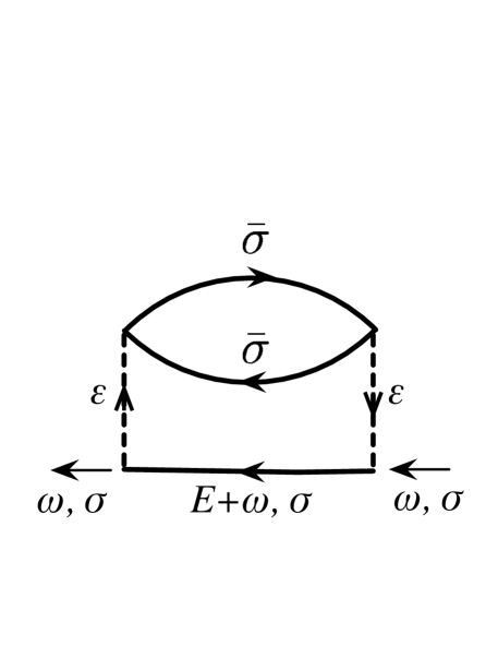
Figure 2: The correlation part of the self-energy at the second-order contribution.

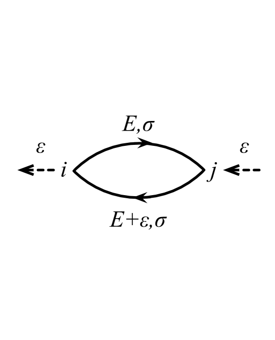
Figure 3: The polarization part

Following the standard perturbation treatment of the Keldysh formulation, we see there is only one diagram contributing to $\Sigma^{R}_{\sigma}$ at the second order (Fig. 2) after eliminating the Hartree-type contribution. The contribution is written as

$$\hat{\Sigma}(t_{1},t_{2})=-i\hbar U^{2}\begin{pmatrix}G^{--}_{12}\Pi^{--}_{21}&-G^{-+}_{12}\Pi^{+-}_{21}\\ -G^{+-}_{12}\Pi^{-+}_{21}&G^{++}_{12}\Pi^{++}_{21}\end{pmatrix}$$ (16)

where $G^{ij}_{12}=G^{ij}(t_{1},t_{2})$ refer to to the unperturbed Green functions (including the Hartree term), whose concrete expressions are found in Appendix A. The polarization matrix $\hat{\Pi}$ is defined by $\Pi^{ij}_{12}=i\hbar\,G^{ij}_{12}G^{ji}_{21}$ (Fig. 3).

As was shown by the current formula in the previous section, we need only the dot spectral function to study quantum transport, hence $\Sigma^{R}$ suffices. Therefore it is more advantageous to work on the RAK-representation, where the polarization parts become

$$\Pi^{R}_{12}=\frac{i\hbar}{2}\left[G^{R}_{12}G^{K}_{21}+G^{K}_{12}G^{A}_{21}\right],$$ (17a)

$$\Pi^{A}_{12}=\frac{i\hbar}{2}\left[G^{A}_{12}G^{K}_{21}+G^{K}_{12}G^{R}_{21}\right],$$ (17b)

$$\Pi^{K}_{12}=\frac{i\hbar}{2}\left[G^{K}_{12}G^{K}_{21}+G^{R}_{12}G^{A}_{21}+G^{A}_{12}G^{R}_{21}\right],$$ (17c)

and their Fourier transformations are given in Appendix B. Accordingly, we can express the retarded self-energy $\Sigma^{R}$ as

$$\Sigma^{R}_{\sigma}(\omega)=-\frac{iU^{2}}{4\pi}\Big{[}I_{1}(\omega)+I_{2}(\omega)\Big{]},$$ (18)

where

$$I_{1}(\omega)=\int^{+\infty}_{-\infty}dE\,G^{R}_{\sigma}(E+\omega)\Pi^{K}_{\bar{\sigma}}(E),$$ (19)

$$I_{2}(\omega)=\int^{+\infty}_{-\infty}dE\,G^{K}_{\sigma}(E+\omega)\Pi^{A}_{\bar{\sigma}}(E).$$ (20)

The above second-order expression of $\Sigma^{R}$ is standard, but it has so far been mainly used for numerical evaluation, quite often restricted for the two-terminal PH symmetric SIAM. We intend to evaluate Eqs. (19,20) analytically for the generic multi-terminal SIAM, along the line employed in Ref. Mühlbacher et al., 2011.

Delegating all the mathematical details to Appendices C and D, we summarize our result of the analytical evaluation of $\Sigma^{R}$ as follows:

$$\Sigma^{R}_{\sigma}(\omega)=\frac{i\gamma U^{2}}{8\pi^{2}(\omega-E_{d\sigma}+i\gamma)}\bigg{[}\frac{\Xi_{1}(\omega-E_{d\sigma})}{\omega-E_{d\sigma}-i\gamma}+\frac{\Xi_{2}(\omega-E_{d\sigma})}{\omega-E_{d\sigma}+3i\gamma}+\frac{\Xi_{3}}{2i\gamma}\bigg{]},$$ (21)

Here, functions $\Xi_{i}$ ($i=1,2,3$) are found to be (using $\zeta_{a\sigma}=\mu_{a}-E_{d\sigma}$),

$$\Xi_{1}(\varepsilon) =\tfrac{2\pi^{2}\varepsilon}{i\gamma}+\sum_{a,b,\beta}\tfrac{4\gamma_{a}\gamma_{b}}{\gamma^{2}}\Big{[}\mathop{\mathrm{Li}_{2}}\nolimits(\tfrac{-\varepsilon+\zeta_{a\sigma}}{\beta\zeta_{b\bar{\sigma}}+i\gamma})+\mathop{\mathrm{Li}_{2}}\nolimits(\tfrac{-\varepsilon-\beta\zeta_{b\bar{\sigma}}}{-\zeta_{a\sigma}+i\gamma})+\tfrac{1}{2}\mathop{\mathrm{Log}}\nolimits^{2}(\tfrac{-\zeta_{a\sigma}+i\gamma}{\beta\zeta_{b\bar{\sigma}}+i\gamma})\Big{]}$$

$$\qquad\qquad+\sum_{a,b,\beta}\tfrac{4\gamma_{a}\gamma_{b}}{\gamma^{2}}\Big{[}\mathop{\mathrm{Li}_{2}}\nolimits(\tfrac{-\varepsilon+\beta\zeta_{a\bar{\sigma}}}{\beta\zeta_{b\bar{\sigma}}+i\gamma})+\tfrac{1}{4}\mathop{\mathrm{Log}}\nolimits^{2}(\tfrac{-\zeta_{a\bar{\sigma}}+i\gamma}{\zeta_{b\bar{\sigma}}+i\gamma})\Big{]},$$ (22a)

$$\Xi_{2}(\varepsilon) =6\pi^{2}-\sum_{a,b,\beta}\tfrac{4\gamma_{a}\gamma_{b}}{\gamma^{2}}\Big{[}\Lambda(\tfrac{\varepsilon-\zeta_{a\sigma}+2i\gamma}{\beta\zeta_{b\bar{\sigma}}+i\gamma})+\Lambda(\tfrac{\varepsilon-\beta\zeta_{b\bar{\sigma}}+2i\gamma}{\zeta_{a\sigma}+i\gamma})+\tfrac{1}{2}\mathop{\mathrm{Log}}\nolimits^{2}(\tfrac{\zeta_{a\sigma}+i\gamma}{\beta\zeta_{b\bar{\sigma}}+i\gamma})\Big{]}$$

$$\qquad\qquad-\sum_{a,b,\beta}\tfrac{4\gamma_{a}\gamma_{b}}{\gamma^{2}}\Big{[}\Lambda(\tfrac{\varepsilon+\beta\zeta_{a\bar{\sigma}}+2i\gamma}{\beta\zeta_{b\bar{\sigma}}+i\gamma})+\tfrac{1}{4}\mathop{\mathrm{Log}}\nolimits^{2}(\tfrac{-\zeta_{a\bar{\sigma}}+i\gamma}{\zeta_{b\bar{\sigma}}+i\gamma})\Big{]},$$ (22b)

$$\Xi_{3} =\left[\sum_{a}\tfrac{2\gamma_{a}}{\gamma}\mathop{\mathrm{Log}}\nolimits\left(\tfrac{-\zeta_{a\bar{\sigma}}+i\gamma}{\zeta_{a\bar{\sigma}}+i\gamma}\right)\right]^{2},$$ (22c)

where the summations over $\beta=\pm 1$ as well as terminals $a,b$ are understood. Function $\mathop{\mathrm{Li}_{2}}\nolimits(z)$ is dilogarithm, whose definition as well as various useful properties are summarized in Appendix C; $\Lambda(z)$ is defined by 

$$\Lambda(z)=\mathop{\mathrm{Li}_{2}}\nolimits(z)+\left[\mathop{\mathrm{Log}}\nolimits(1-z)-\mathop{\mathrm{Log}}\nolimits(z-1)\right]\mathop{\mathrm{Log}}\nolimits z.$$ (23)

Analytical formula $\Sigma^{R}$ given in Eqs. (21) and (22) constitutes the main result of the present paper. Consequently, the nonequilibrium spectral function of the multi-terminal SIAM is given analytically for full range of frequency and bias voltage, once one chooses $n_{\sigma}$ to satisfy Eq. (6). The result also applies to a more involved structured system, such as an interferometer embedding a quantum dot, by simply replacing $\epsilon_{d}$ and $\gamma_{a}$ to take account of those geometric effect.

IV Various analytical behaviors

Having obtained an explicit analytical form of the second-order self-energy $\Sigma^{R}(\omega)$ at arbitrary frequency and bias voltage, we now examine its various limiting behaviors. Most of those limiting behaviors have been known for the two-terminal PH symmetric SIAM, so it’s assuring to reproduce those expressions in such a case. Simultaneously, our results below provide multi-terminal, PH asymmetric extensions of those asymptotic results.

IV.1 Equilibrium dot with and without the PH symmetry

We can reproduce the equilibrium result by setting all the chemical potentials equal, $\mu_{a\sigma}=E_{d\sigma}=\epsilon_{d}+Un_{\bar{\sigma}}$. Then we immediately see $\Xi_{3}=0$ and

$$\Xi_{1}=8\cdot\big{[}\tfrac{\pi^{2}}{4}(\tfrac{\varepsilon_{\sigma}}{i\gamma})+3\mathop{\mathrm{Li}_{2}}\nolimits(\tfrac{-\varepsilon_{\sigma}}{i\gamma})\big{]},$$ (24)

$$\Xi_{2}=8\cdot\big{[}\frac{3\pi^{2}}{4}-3\Lambda(\tfrac{\varepsilon_{\sigma}+2i\gamma}{i\gamma})\big{]},$$ (25)

where $\varepsilon_{\sigma}=\omega-E_{d\sigma}$. As a result, the correlation part of the self-energy in equilibrium becomes

$$\Sigma^{R}_{\sigma}(\omega)=\frac{i\gamma U^{2}}{\pi^{2}(\varepsilon_{\sigma}+i\gamma)}\bigg{[}\frac{\tfrac{\pi^{2}}{4}(\tfrac{\varepsilon_{\sigma}}{i\gamma})+3\mathop{\mathrm{Li}_{2}}\nolimits(\tfrac{-\varepsilon_{\sigma}}{i\gamma})}{\varepsilon_{\sigma}-i\gamma}$$

$$\qquad\qquad\qquad\qquad+\frac{\tfrac{3\pi^{2}}{4}-3\Lambda(2+\tfrac{\varepsilon_{\sigma}}{i\gamma})}{\varepsilon_{\sigma}+3i\gamma}\bigg{]}.$$ (26)

The PH symmetric case in particular corresponds to $\varepsilon_{\sigma}=\omega$. It reproduces the perturbation results by Yamada and Yoshida Yamada (1975a, b); Yoshida and Yamada (1975) up to the second-order of $U$, when we expand the above for small $\omega$. The PH symmetric result is indeed identical with the one obtained in Ref. Mühlbacher et al., 2011 for arbitrary frequency (See also Eq. (27) below).

IV.2 Nonequilibrium PH symmetric dot connected with two terminals

Mühlbacher et al. (2011) have evaluated analytically the self-energy and the spectral function for the two-terminal PH symmetric SIAM. In our notation, it corresponds to the case $\gamma_{L}=\gamma_{R}=\gamma/2$, and $E_{d\sigma}=0$. When we parametrize the two chemical potentials by $\mu_{a}=\zeta_{a\sigma}=aeV/2$ with $a=\pm 1$ in Eqs. (22), the self-energy can be written as

$$\Sigma^{R}_{\sigma}(\omega)=\frac{i\gamma U^{2}}{8\pi^{2}(\omega+i\gamma)}\left[\frac{\Xi_{1}(\omega)}{\omega-i\gamma}+\frac{\Xi_{2}(\omega)}{\omega+3i\gamma}\right],$$ (27)

where

$$\Xi_{1}=\tfrac{2\pi^{2}\omega}{i\gamma}+6\sum_{a,b}\Big{[}\mathop{\mathrm{Li}_{2}}\nolimits(\tfrac{-\omega+aeV/2}{beV/2+i\gamma})+\tfrac{1}{4}\mathop{\mathrm{Log}}\nolimits^{2}(\tfrac{-aeV/2+i\gamma}{beV/2+i\gamma})\Big{]},$$

$$\Xi_{2}=6\pi^{2}-6\sum_{a,b}\Big{[}\Lambda(\tfrac{\omega-aeV/2+2i\gamma}{beV/2+i\gamma})+\frac{1}{4}\mathop{\mathrm{Log}}\nolimits^{2}(\tfrac{aeV/2+i\gamma}{beV/2+i\gamma})\Big{]}.$$

The above result are identical with what Ref. Mühlbacher et al., 2011 obtained.

IV.3 Expansion of small bias and frequency

We now employ the small-parameter expansion of $\Sigma^{R}$ around the half-filled equilibrium system. Here we assume parameters $\zeta_{a\sigma}=\mu_{a}-E_{d\sigma}$ and $\varepsilon_{\sigma}=\omega-E_{d\alpha}$ are much smaller than the total relaxation rate $\gamma$. The expansion of $\Xi_{1}$ is found to contain the first- and second-order terms regarding $\zeta_{a\sigma}$ and $\varepsilon_{\sigma}$, while $\Xi_{2,3}$ do only the second-order terms. Therefore the result of the expansion up to the second-order of these small parameters is presented as

$$\Sigma^{R}_{\sigma}(\omega)\approx\frac{iU^{2}}{8\pi^{2}\gamma}\left[\Xi_{1}-\frac{\Xi_{2}}{3}-\frac{\Xi_{3}}{2}\right].$$ (28)

Functions $\Xi_{i}$ can be expanded straightforwardly by using the Taylor expansion of dilogarithm in Appendix C. They are found to behave

$$\Xi_{1}(\varepsilon)\approx 8\,\Big{[}\frac{(\pi^{2}-12)\varepsilon+4\bar{\mu}}{4i\gamma}+\frac{3\varepsilon^{2}+9\overline{\mu^{2}}-6\varepsilon\bar{\mu}-2\bar{\mu}^{2}}{4(i\gamma)^{2}}\big{]},$$ (29)

$$\Xi_{2}(\varepsilon)\approx-8\,\Big{[}\frac{3(-\varepsilon^{2}+2\varepsilon\bar{\mu}+2\bar{\mu}^{2}-\overline{\mu^{2}}-2\overline{\mu^{2}})}{4(i\gamma)^{2}}\Big{]}$$ (30)

$$\Xi_{3}\approx\frac{16\bar{\mu}^{2}}{(i\gamma)^{2}},$$ (31)

where $\bar{\mu}$ is defined in Eq. (15) and we have introduced

$$\overline{\mu^{2}}=\sum_{a}\frac{\gamma_{a}}{\gamma}\mu_{a}^{2}=\bar{\mu}^{2}+(\delta\mu)^{2}.$$ (32)

Combining all of these, we reach the small bias/frequency behavior of the self-energy $\Sigma^{R}_{\sigma}$ as

$$\Sigma^{R}_{\sigma}(\omega)\approx\frac{U^{2}}{\pi^{2}\gamma^{2}}\left[(\tfrac{\pi^{2}}{4}-3)(\omega-E_{d\sigma})+\bar{\mu}\right]$$

$$\qquad\qquad-\frac{iU^{2}}{2\pi^{2}\gamma^{3}}\Big{[}(\omega-\bar{\mu})^{2}+3\,(\delta\mu)^{2}\Big{]}.$$ (33)

Small bias expansion of $\mathop{\mathrm{Im}}\nolimits\Sigma^{R}$ for the two-terminal system has been discussed and determined by the argument based on the Ward identity. Oguri (2002) The dependence appearing in Eq. (33) fully conforms to it (except for the presence of the bare interaction instead of the renormalized one). Indeed, correspondence is made clear by noting the parameters $\bar{\mu}$ and $\overline{\delta\mu^{2}}$ for the two-terminal case become

$$\bar{\mu}=\frac{\gamma_{L}\mu_{L}+\gamma_{R}\mu_{R}}{\gamma};\quad(\delta\mu)^{2}=\frac{\gamma_{L}\gamma_{R}}{\gamma^{2}}(eV)^{2}.$$ (34)

The presence of linear term in $\omega$ and $V$ for the two-terminal PH asymmetric SIAM was also emphasized recently. Aligia (2012)

IV.4 Large bias voltage behavior

One expects naively that the limit of large bias voltage $eV\to\infty$ corresponds to the high temperature limit $T\to\infty$ in equilibrium; it was shown to be so for the two-terminal PH symmetric SIAM. Oguri (2002) We now show that the same applies to the multi-terminal SIAM where bias voltages of the leads are pairwisely large, i.e., half of them are positively large, and the others are negatively large.

In the large bias voltage limit, all the arguments of dilogarithm functions appearing in Eqs. (22) become $\pm 1$, where the values of dilogarithm are known (see Appendix C). Accordingly, the pairwisely large bias limit of $\Xi_{i}$ is found to be

$$\Xi_{1}(\varepsilon)\approx\frac{2\pi^{2}(\varepsilon-i\gamma)}{i\gamma},$$ (35)

$$\Xi_{2}(\varepsilon)\approx-4\pi^{2},$$ (36)

$$\Xi_{3}\approx 0.$$ (37)

Correspondingly, the retarded self-energy becomes

$$\Sigma^{R}_{\sigma}(\omega)\approx\frac{U^{2}/4}{\omega-E_{d\sigma}+3i\gamma}$$ (38)

It shows that the result of the multi-terminal SIAM is the same with that of the two-terminal PH symmetric SIAM except for a frequency shift. Accordingly, the retarded Green function $G^{R}(\omega)$ in this limit is given by

$$G^{R}_{\sigma}(\omega)\approx\frac{1}{\omega-E_{d\sigma}+i\gamma-\frac{U^{2}/4}{\omega-E_{d\sigma}+3i\gamma}}.$$ (39)

The form indicates that for sufficiently strong interaction $U\gtrsim 2\gamma$, the dot spectral function has two peaks at $E_{d\sigma}\pm U/2=\epsilon_{d}+U(n_{\bar{\sigma}}\pm 1/2)$ with broadening $2\gamma$, so the system is driven into the the Coulomb blockade regime. On the other hand, for weak interaction $U<2\gamma$, it has only one peak with two different values of broadening that reduce to $\gamma$ and $3\gamma$ in the $U\to 0$ limit.

What is the role of the current preservation condition Eq. (6) in this limit? It just determines the dot occupation number explicitly. In fact, the condition becomes

$$n_{\sigma}=\frac{-1}{\pi}\sum_{a}\frac{\gamma_{a}}{\gamma}\mathop{\mathrm{Im}}\nolimits\int^{(\mu_{a}-E_{d\sigma})/\gamma}_{-\infty}\frac{dx}{x+i-\frac{u^{2}}{x+3i}}$$ (40)

with $u=U/(2\gamma)$, and $n_{\sigma}$ is independent of the interaction strength because bias voltage sets the largest scale. One can evaluate the above integral exactly to have

$$\int\frac{dx}{x+i-\frac{u^{2}}{x+3i}}=\sum_{s=\pm 1}\frac{\sqrt{1-u^{2}}+s}{2\sqrt{1-u^{2}}}\mathop{\mathrm{Log}}\nolimits(x-\alpha_{s}),$$ (41)

where $\alpha_{\pm}=-2i\pm i\sqrt{1-u^{2}}$. As a result, expanding it up to the second order of $u$ leads to

$$n_{\sigma}\approx\sum_{a}\frac{\gamma_{a}}{\gamma}\theta(\mu_{a})-\frac{1}{\pi}\sum_{a}\frac{\gamma_{a}}{\mu_{a}}.$$ (42)

The first term corresponds to the occupation number that one expects naturally from the effective distribution $\bar{f}$; it corresponds, for instance, $\gamma_{L}/(\gamma_{L}+\gamma_{R})$ for the two-terminal dot with $\mu_{R}<0<\mu_{L}$ with $|\mu_{R,L}|\to\infty$. The second term is the deviation from it, which is proportional to the average of the inverse chemical potential weighted by the leads.

V Nonequilibrium spectral function

We now turn our attention to the behavior of the nonequilibrium dot spectral function, using our analytical expression of the self-energy Eqs. (21,22). Below we particularly focus our attention on the two cases: the two-terminal PH asymmetric SIAM where current preservation has been an issue, and the multi-terminal PH symmetric SIAM where the role of multiple leads has been raising questions. In all of the calculations below, we have checked numerically the validity of the spectral weight sum rule at each configuration of bias voltages.

V.1 Self-consistent current-preserving calculation

As was emphasized in Sec. II.2, when a dot system does not retain the PH symmetry, the stationary current is not automatically conserved and one must impose the current preservation condition Eq. (6) explicitly. As the right-hand side of Eq. (6) also depends on the dot occupation number $n_{\sigma}$, this requires us to determine $n_{\sigma}$ self-consistently by using the retarded Green function in a certain approximation — the second-order perturbation theory in the present case.

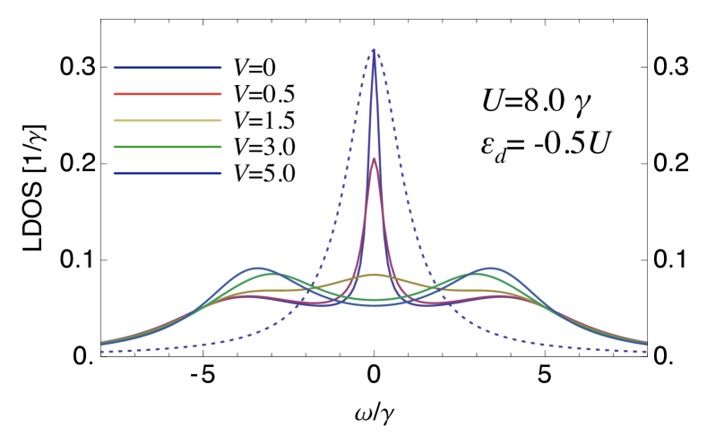
Figure 4: (Color online) Nonequilibrium dot spectral function of the two-terminal PH symmetric SIAM ($\epsilon_{d}=-U/2$) at finite bias voltage $eV=0,0.5,1.5,3.0,5.0\gamma$. The interaction strength is chosen as $U=8\gamma$. The dotted line represents the result of $U=0$ and $V=0$.

Figure 4 shows the result of nonequilibrium dot spectral function of the two-terminal PH symmetric SIAM at bias voltage $eV=0,0.5,1.5,3.0$, and $5.0\gamma$, which is essentially the same result with Ref. Mühlbacher et al., 2011 (of a different set of parameters). The occupation number is fixed to be $n_{\sigma}=1/2$ in this case, so its self-consistent determination is unnecessary. The results were compared favorably with those obtained by diagrammatic quantum Monte Carlo calculations Mühlbacher et al. (2011); a relatively good quantitative agreement was observed up to $U\sim 8\gamma$ (where the Bethe ansatz Kondo temperature $k_{B}T_{K}=0.055\gamma$ Tsvelick and Wiegmann (1983a) while the estimated half width of the Kondo resonance $k_{B}\tilde{T}_{K}=0.23\gamma$) and bias voltage $V\lesssim 2\gamma$. Applying bias voltage gradually suppresses the Kondo resonance without splitting it, and the two peaks at $\pm U/2$ are developed at larger bias voltages, which corresponds to the discussion in the previous section.

Figure 5 shows the result of our self-consistent calculation of the nonequilibrium spectral function for the two-terminal PH asymmetric SIAM at (a) $\epsilon_{d}=-0.625U$ and (b) $\epsilon_{d}=-0.75U$. A paramagnetic-type solution is assumed in determining $n_{\sigma}$. As in the PH symmetric SIAM, one sees increasing bias voltage not split but suppress the Kondo resonance while it develops a peak around $E_{d}-U/2$. The Kondo resonance peak is suppressed more significantly at $\epsilon_{d}=-0.625U$ than at $-0.75U$, because the Kondo temperature of the former ($k_{B}T_{K}\approx 0.067\gamma$; $k_{B}\tilde{T}_{K}\approx 0.49\gamma$) is smaller than that of the latter ($k_{B}T_{K}\approx 0.12\gamma$; $k_{B}\tilde{T}_{K}\approx 0.58\gamma$). An interesting feature of the PH asymmetric SIAM is that spectral weight of the Kondo resonance seems shifting gradually toward $E_{d}+U/2$ with increasing bias voltage, without exhibiting a three-peak structure in the PH symmetric case. This suggests a strong spectral mixing between the Kondo resonance and a Coulomb peak at finite bias voltage. Because of it, the interval of the two peaks at finite bias is observed as roughly $U/2$ and gets widened up to $U$ for larger $eV$. The bias dependence somehow looks similar to what was obtained by assuming equilibrium noninteracting effective distribution for $n_{\sigma}$ Matsumoto (2000) (which is hard to justify in our opinion), though we emphasize our present calculation only relies on the current-preservation condition without using any further assumption. It is remarked that the effect shown by bias voltage is quite reminiscent of finite temperature effect that was observed in the PH asymmetric SIAM in equilibrium Horvatić et al. (1987).

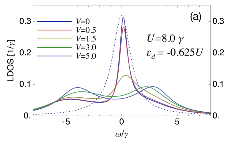
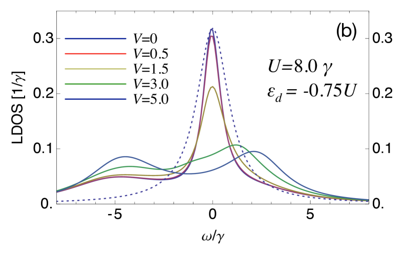
Figure 5: (Color online) Nonequilibrium dot spectral function of the PH asymmetric SIAM at (a) $\epsilon_{d}=-0.625U$, and (b) $\epsilon_{d}=-0.75U$. All the other parameters are the same with Fig. 4. As an eye guide, the PH symmetric result of $U=0$ and $V=0$ is shown as a dotted line.

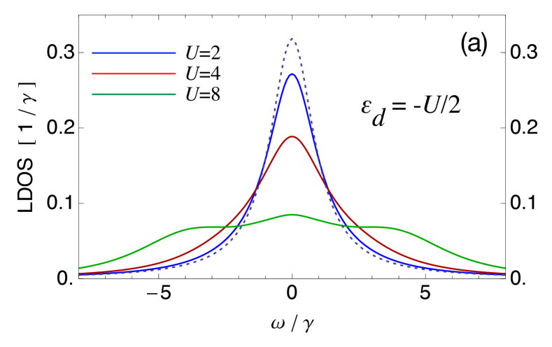
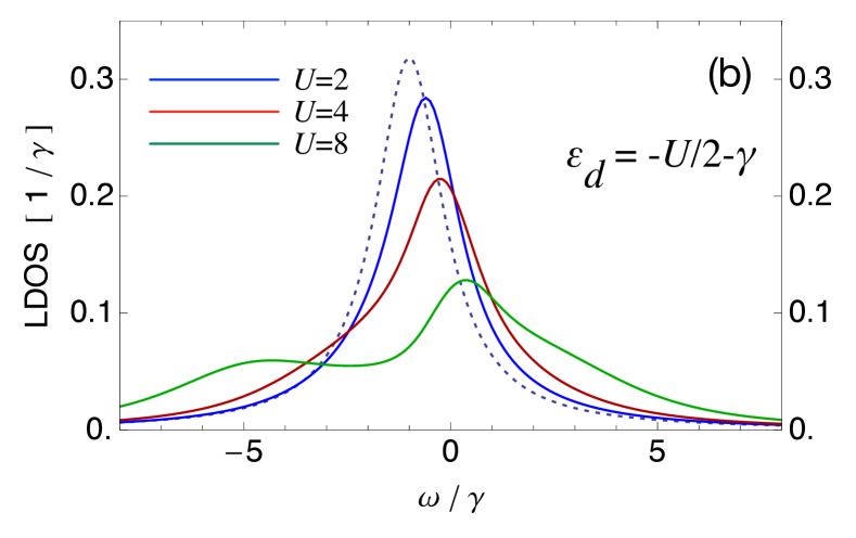
Figure 6: (Color online) Nonequilibrium dot spectral function for different values of interaction strength at bias voltage $eV=1.5\gamma$. Results of the interaction strengths $U=2\gamma$, $4\gamma$, and $8\gamma$ are shown, while dotted lines refer to the noninteracting case as an eye guide. (a) spectral function of the PH symmetric SIAM at $\epsilon_{d}=-U/2$. (b) spectral function of the PH asymmetric SIAM at $\epsilon_{d}=-U/2-\gamma$.

More insight can be gained by examining how the spectral structure depends on the interaction strength at finite bias voltage. Figures 6 (a,b) show a structural crossover from a noninteracting resonant peak (the dotted line) to correlation peaks, for (a) the PH symmetric SIAM $\epsilon_{d}=-U/2$, and (b) the PH asymmetric SIAM $\epsilon_{d}=-U/2-\gamma$. The PH symmetric SIAM shows introducing $U$ leads to developing the correlation two peaks as well as the Kondo peak that is suppressed by finite bias voltage. In contrast, the bias voltage effect on the PH asymmetric SIAM is more involved, because the Kondo resonance is apparently shifted and mixed with one of the correlation peaks, eventually showing the two-peak structure at $E_{d}\pm U/2$ in large bias voltage limit.

V.2 Multi-terminal PH symmetric SIAM

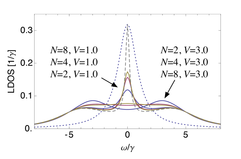
Figure 7: (Color online) Nonequilibrium dot spectral function for the PH symmetric multi-terminal dot ($N=2,4$, and $8$). Other parameters are chosen as the same as in Fig. 4. The dotted line correspond to the two-terminal noninteracting unbiased case, while the dashed line, to the two-terminal interacting unbiased case.

To examine finite bias affects further and see particularly how the presence of multi-terminals affects the nonequilibrium spectral function, we configure a special setup of the multi-terminal SIAM that preserves the PH symmetry: the dot is connected with $N$ identical terminals, with bias levels being distributed equidistantly between $-V/2$ and $+V/2$, and each of relaxation rates is set to be $\gamma/N$. The latter ensures that the unbiased spectral function is the same, hence the Kondo temperature. Results of the nonequilibrium spectral function are shown in Fig. 7. Again, we confirm that no splitting of the Kondo resonance is observed in this multi-terminal setting. One sees further that the increasing the number of terminals enhances the Kondo resonance. This can be understood by weakening the bias suppression effect on the Kondo resonance for a larger $N$. More precisely, one may estimate the suppressing effect from small bias behavior Eq. (33). Hence $\delta\mu$ is a control parameter. In the present multi-terminal PH symmetric setting, the quantity $\delta\mu$ is found to be

$$\delta\mu=V\sqrt{\frac{N+1}{12(N-1)}}.$$ (43)

Therefore $\delta\mu$ decreases with increasing $N$, which results in weakening the suppression and enhancing the Kondo resonance for a larger $N$.

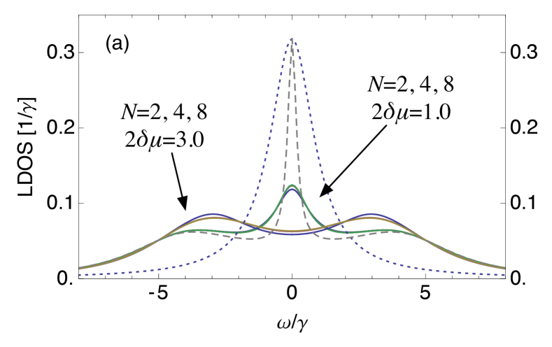
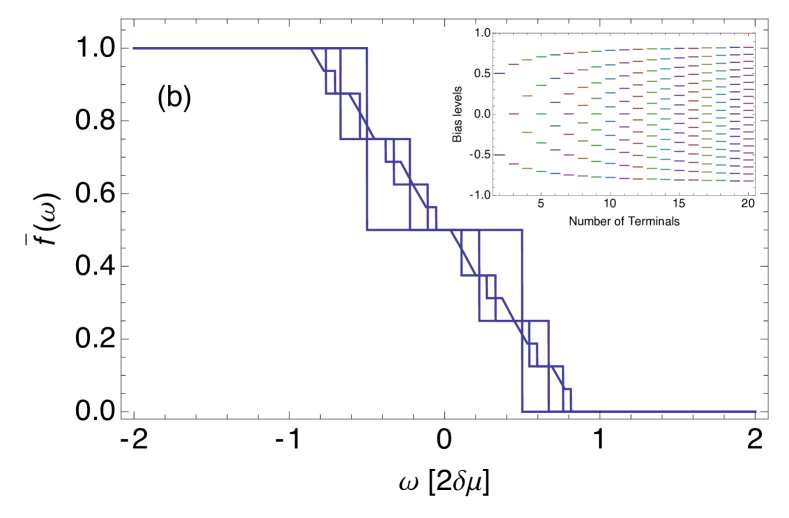
Figure 8: (Color online) (a) Nonequilibrium spectral function for the PH symmetric multi-terminal dot with fixing $\delta\mu$ ($N=2,4,8$). Other parameters are the same as in Fig. 7. (b) The effective Fermi distribution $\bar{f}(\omega)$ at zero temperature for the PH symmetric multi-terminal dot ($N=2,4,8,16$). The inset shows relative locations of bias levels with fixed $\delta\mu$ as a function of the number of terminals.

The preceding argument also tells us that if the spectral function bears any multi-terminal signatures at all, they would be more conspicuous by examining it with fixing $\delta\mu$ rather than $V$. This is done in Fig. 8 (a); Figure 8 (b) shows how the effective dot distribution $\bar{f}(\omega)$ and the relative locations of bias levels (in the inset) evolve for a fixed $\delta\mu$ when $N$ increases. No multi-terminal signature in the nonequilibrium spectral function is seen in Fig. 8 (a); results of different $N$ actually collapse, not only around zero frequency but in the entire frequency range. It suggests that the suppression of the Kondo resonance deeply correlates the development of Coulomb peaks, and a mixing between those spectral weight is important. The parameter $\delta\mu$ controls a crossover from the Kondo resonance to the Coulomb blockade structure. We may also understand the similarity between bias effect and temperature effect by the connection through the large $N$ limit of the effective Fermi distribution $\bar{f}(\omega)$, as shown in Fig. 8 (b).

V.3 Finite bias effect on the spectral function: issues and speculation

Although there is a consensus that bias voltage starts suppressing the Kondo peak, and eventually destroys it with developing the two Coulomb peaks when bias voltage is much larger than the Kondo temperature, there is a controversy as to whether the Kondo resonance peak will be split or not in the intermediate range of bias voltage. All the results obtained by the second-order perturbation consistently indicate that there is no split of the Kondo resonance; finite bias voltage starts to suppress the Kondo resonance, and develops the two Coulomb blockade peaks by shifting the spectral weight from the Kondo resonance. We should mention that some other approximations draw a different conclusion. Here we make a few remarks on apparent discrepancy seen in various theoretical approaches as well as experiments, as well as some speculation based on our results.

Typically, several approaches that rely on the infinite $U$ limit, notably non-crossing approximation, equation of motion method, and other approaches investigating the Kondo Hamiltonian, observed the splitting of the Kondo resonance under finite bias voltage Meir et al. (1993); Wingreen and Meir (1994); Shah and Rosch (2006). Those results, however, have to be interpreted with great care, in our view. Generally speaking, the spectral function obtained by those approaches does not obey the spectral weight sum rule: ignoring the doubly occupied state typically leads to the sum rule $-\int^{\infty}_{-\infty}\mathop{\mathrm{Im}}\nolimits G^{R}_{\sigma}(\omega)/\pi=1/2$ Meir et al. (1993), rather than the correct value. Therefore only half of the spectral weight can be accounted for in those methods. Simultaneously, such (false) sum rule in conjugation with the bias-suppression of the Kondo resonance cannot hep but lead to a two-peak structure of the spectrum within the range of attention. Splitting of the Kondo resonance might be an artifact of the approximation. Not fulfilling the correct sum rule, those approaches may not be able to distinguish whether finite bias will split the Kondo resonance or simply suppresses it with developing the Coulomb peaks. As for the two-terminal PH symmetric SIAM, fourth-order contribution regarding the Coulomb interaction $U$ has been evaluated numerically Fujii and Ueda (2003, 2005); Hamasaki (2007). The results seem unsettled, though. While Fujii and Ueda (2003, 2005) suggested the fourth-order term may yield the splitting of the Kondo resonance in the intermediate bias region $k_{B}\tilde{T}_{K}\lesssim eV\lesssim U$ for sufficiently large interaction $U/\gamma\gtrsim 4$, which the second-order calculation fails to report, another numerical study indicates that the spectral function remains qualitatively the same with the second-order result Hamasaki (2007). Experimental situation is not so transparent, either. While the splitting of the Kondo resonance was reported in a three-terminal conductance measurement in a quantum ring system Leturcq et al. (2005), a similar spitting observed in the differential conductivity was attributed to being caused by a spontaneous formation of ferromagnetic contacts, not purely to bias effect Nygard et al. (2004). It is also pointed out that it has been recently recognized that the Rashba spin-orbit coupling induces spin polarization nonmagnetically in a quantum ring system with a dot when applying finite bias voltage feng Sun and Xie (2006); Crisan et al. (2009); Taniguchi and Isozaki (2012); hence such spin magnetization might possibly lead to the splitting of the Kondo resonance.

The Kondo resonance is a manifestation of singlet formation between the dot and the lead electrons. One may naively think that when several chemical potentials are connected with the dot, such singlet formation would take place at each lead separately, causing multiple Kondo resonances. The results of the multi-terminal PH symmetric SIAM presented in the previous section tempt us to speculate a different picture. Let us suppose that (almost) the same dot distribution function $f_{\text{dot}}(\omega)=G^{-+}(\omega)/(2i\pi)$ is realized for a fixed $\delta\mu$ with a different terminal number $N$, as Fig. 8 (a) suggests. Note the assumption is fully consistent to the Ward identity for low bias, but it invalidates a quasiparticle ansatz $-\bar{f}(\omega)\mathop{\mathrm{Im}}\nolimits G^{R}(\omega)/\pi$ that explicitly depends on $N$. In the large $N$ limit with a fixed $\delta\mu$, the effective Fermi distribution $\bar{f}(\omega)$ resembles the Fermi distribution at finite temperature $k_{B}T\sim\delta\mu$. Accordingly bias voltage may well give effect similar to finite temperature. It is seen in low and large bias limit for a dot with or without the PH symmetry. It implies that a dot electron cannot separately form a singlet with the lead at each chemical potential, because it needs to implicates states at different chemical potentials through coupling with other leads. Our second-order perturbation results seem to support this view.

VI Conclusion

In summary, we have evaluated analytically the second-order self-energy and Green function for a generic multi-terminal single impurity Anderson model in nonequilibrium. Various limiting behaviors have been examined analytically. Nonequilibrium spectral function that preserves the current is constructed and is checked to satisfy the spectral weight sum rule. The multi-terminal effect is examined for the PH-symmetric SIAM, particularly. Within the validity of the present approach, it is shown that the Kondo peak is not split due to bias voltage. It is found that most of the finite bias effect is similar to that of finite temperature in low- and high-bias limits with and without the PH symmetry. Such nature could be understood by help of the Ward identity and the connection through the $N\gg 1$ terminal limit. The present analysis serves as a viable tool that can cover a wide range of experimental situations. Although there is still a chance that high-order contributions might generate a new effect such as split Kondo resonances in a limited range of parameters, it is believed that the second-order perturbation theory can capture the essence of the Kondo physics in most of realistic situations. Moreover, having a concrete analytical form that satisfies both the current conservation and the sum rule, the present work provides a good, solid, workable result that more sophisticated future treatment can base on.

Appendix A Noninteracting Green functions with finite bias

We start with the nonequilibrium Green function $G$ without the Coulomb interaction on the dot. Its Keldysh structure is specified by

$$G_{\sigma}(\omega)=\begin{pmatrix}\omega-\epsilon_{d}+i\gamma(1-2\bar{f})&+2i\gamma\bar{f}\\ -2i\gamma(1-\bar{f})&\!\!\!\!\!\!\!-(\omega-\epsilon_{d})+i\gamma(1-2\bar{f})\end{pmatrix}^{-1},$$ (44)

where $\bar{f}$ is the effective dot distribution defined in Eq. (5). We incorporate the Hartree-type diagram into the unperturbed part by replacing $\epsilon_{d}$ to $\epsilon_{d}\mapsto E_{d\sigma}=\epsilon_{d}+Un_{\bar{\sigma}}$. Note $n_{\bar{\sigma}}$ is the exact dot occupation that needs to be determined consistently later. After mapping to the RAK representation, those components are given by

$$G^{R,A}_{\sigma}(\omega)=\frac{1}{\omega-E_{d\sigma}\pm i\gamma},$$ (45)

$$G^{K}_{\sigma}(\omega)=[1-2\bar{f}(\omega)]\left[G^{R}_{\sigma}(\omega)-G^{A}_{\sigma}(\omega)\right].$$ (46)

The function $1-2\bar{f}(\omega)$ reduces to $\sum_{a}(\gamma_{a}/\gamma)\mathop{\mathrm{sgn}}\nolimits(\omega-\mu_{a})$ at zero temperature.

Appendix B Nonequilibrium polarization part

Taking the Fourier transformation of Eqs. (17), using Eq. (46), and making further manipulations, we can rewrite $\Pi^{R}$ and $\Pi^{K}$ as

$$\Pi^{R}(\varepsilon) =\sum_{a}\frac{\gamma_{a}}{\gamma}\frac{\gamma B_{aa}(\varepsilon)}{\pi\varepsilon(\varepsilon+2i\gamma)}=\left[\Pi^{A}(\varepsilon)\right]^{*},$$ (47)

$$\Pi^{K}(\varepsilon) =2i\sum_{a,b}\frac{\gamma_{a}\gamma_{b}}{\gamma^{2}}\coth\tfrac{\beta(\varepsilon-\mu_{ab})}{2}\mathop{\mathrm{Im}}\nolimits\left[\frac{\gamma B_{ab}(\varepsilon)}{\pi\varepsilon(\varepsilon+2i\gamma)}\right],$$ (48)

where $\mu_{ab}=\mu_{a}-\mu_{b}$, $\beta$ is the inverse temperature, and $B_{ab}(\varepsilon)$ is given by

$$B_{ab}(\varepsilon)=\int\!\!d\varepsilon^{\prime}\!\left[f_{b}(\varepsilon^{\prime})-f_{a}(\varepsilon^{\prime}+\varepsilon)\right]\!\left[G^{A}(\varepsilon^{\prime})-G^{R}(\varepsilon^{\prime}+\varepsilon)\right].$$ (49)

In the present work, we are interested in the zero temperature limit, for which $\coth(\beta x)$ becomes $\mathop{\mathrm{sgn}}\nolimits(x)$. The function $B_{ab}$ in this limit is evaluated as (with $\zeta_{a\sigma}=\mu_{a}-E_{d\sigma}$)

$$B_{ab}(\varepsilon)=-\log\left(\frac{\varepsilon-\zeta_{a\sigma}+i\gamma}{-\zeta_{b\sigma}+i\gamma}\right)-\log\left(\frac{\varepsilon+\zeta_{b\sigma}+i\gamma}{\zeta_{a\sigma}+i\gamma}\right).$$ (50)

This corresponds to a multi-terminal extension of the result obtained for the two-terminal PH symmetric SIAM.

Appendix C Dilogarithm with a complex variable

To complete evaluating the remaining integral over $E$ of Eqs. (19,20), we take full advantage of various properties of dilogarithm function $\mathop{\mathrm{Li}_{2}}\nolimits(z)$. A concrete integral formula we have utilized will be given in Appendix D. For the sake of completeness, we here collect its definition and properties necessary to complete our evaluation.

Definition

Dilogarithm $\mathop{\mathrm{Li}_{2}}\nolimits(z)$ with a complex argument $z\in\mathbb{C}$ is not so commonly found in literature. As it is a multi-valued function, we need to specify its branch structure properly. One way to define dilogarithm $\mathop{\mathrm{Li}_{2}}\nolimits(z)$ all over the complex plane consistently is to use the integral representation

$$\mathop{\mathrm{Li}_{2}}\nolimits(z)=-\int^{z}_{0}dt\,\frac{\mathop{\mathrm{Log}}\nolimits(1-t)}{t}.$$ (51)

The multivaluedness of dilogarithm $\mathop{\mathrm{Li}_{2}}\nolimits$ originates from logarithm in the integrand. Here we designate the principal value of logarithm as $\mathop{\mathrm{Log}}\nolimits$, which is defined by

$$\mathop{\mathrm{Log}}\nolimits z=\ln|z|+i\mathop{\mathrm{Arg}}\nolimits z;\quad\text{(for $-\pi<\mathop{\mathrm{Arg}}\nolimits z\leq\pi$)}.$$ (52)

According to Eq. (51), $\mathop{\mathrm{Li}_{2}}\nolimits(z)$ has a branch-cut just above the real axis of $x>1$. Accordingly, its values just above and below the real axis are different for $x>1$: $\mathop{\mathrm{Li}_{2}}\nolimits(x-i\eta)=\mathop{\mathrm{Li}_{2}}\nolimits(x)$ but $\mathop{\mathrm{Li}_{2}}\nolimits(x+i\eta)=\mathop{\mathrm{Li}_{2}}\nolimits(x)+2i\pi\ln x$. Some special values are known analytically. We need $\mathop{\mathrm{Li}_{2}}\nolimits(0)=0$, $\mathop{\mathrm{Li}_{2}}\nolimits(1)=\pi^{2}/6$, $\mathop{\mathrm{Li}_{2}}\nolimits(-1)=-\pi^{2}/12$ and $\mathop{\mathrm{Li}_{2}}\nolimits(2)=\pi^{2}/4-i\pi\ln 2$ for evaluation later.

Functional relations

Dilogarithm $\mathop{\mathrm{Li}_{2}}\nolimits(z)$ has interesting symmetric properties regarding its argument $z$; values at $z$, $1-z$, $1/z$, $1/(1-z)$, $(z-1)/z$ and $z/(z-1)$ are all connected with one another. Those points are ones generated by symmetric operations $S$ and $T$ defined by

$$Sz=\frac{1}{z};\quad Tz=1-z,$$ (53)

and $\{I,S,T,ST,TS,TST\}$ forms a group. Other operations correspond to

$$STz=\frac{1}{1-z};\quad TSz=\frac{z-1}{z},$$ (54)

$$TSTz=STSz=\frac{z}{z-1}.$$ (55)

Applying a series of integral transformations in Eq. (51), one can connect the values of dilogarithm at these values with one another Maximon (2003). Note, those functional relations are usually presented only for real arguments. Extending them for complex variables needs examining its branch-cut structure carefully. By following and extending the derivations in Ref Maximon, 2003 for complex $z\in\mathbb{C}$, we prove that the following functional relations are valid for any complex variable $z$.

$$\mathop{\mathrm{Li}_{2}}\nolimits(Sz)=-\mathop{\mathrm{Li}_{2}}\nolimits(z)-\tfrac{\pi^{2}}{6}-\tfrac{1}{2}\left[\mathop{\mathrm{Log}}\nolimits(TSz)-\mathop{\mathrm{Log}}\nolimits(Tz)\right]^{2},$$ (56)

$$\mathop{\mathrm{Li}_{2}}\nolimits(Tz)=-\mathop{\mathrm{Li}_{2}}\nolimits(z)+\tfrac{\pi^{2}}{6}-\mathop{\mathrm{Log}}\nolimits(Tz)\mathop{\mathrm{Log}}\nolimits z,$$ (57)

$$\mathop{\mathrm{Li}_{2}}\nolimits(TSTz)=-\mathop{\mathrm{Li}_{2}}\nolimits(z)-\tfrac{1}{2}\mathop{\mathrm{Log}}\nolimits^{2}(STz)$$

$$\qquad\qquad\qquad-[\mathop{\mathrm{Log}}\nolimits(Tz)+\mathop{\mathrm{Log}}\nolimits(STz)]\mathop{\mathrm{Log}}\nolimits z,$$ (58)

$$\mathop{\mathrm{Li}_{2}}\nolimits\big{(}TSz\big{)}=\mathop{\mathrm{Li}_{2}}\nolimits(z)-\tfrac{\pi^{2}}{6}$$

$$\qquad\qquad\qquad-\tfrac{1}{2}\mathop{\mathrm{Log}}\nolimits^{2}(Sz)-\mathop{\mathrm{Log}}\nolimits(Sz)\mathop{\mathrm{Log}}\nolimits(Tz),$$ (59)

$$\mathop{\mathrm{Li}_{2}}\nolimits\big{(}STz\big{)}=\mathop{\mathrm{Li}_{2}}\nolimits(z)+\tfrac{\pi^{2}}{6}$$

$$\qquad\qquad\qquad+\tfrac{1}{2}\mathop{\mathrm{Log}}\nolimits^{2}(Tz)+\mathop{\mathrm{Log}}\nolimits(Tz)\mathop{\mathrm{Log}}\nolimits(TSTz).$$ (60)

To our knowledge, the above form of extension of functional relations of dilogarithm has not been found in literature.

The Taylor expansion

To examine various limiting behaviors, we need the Taylor expansion of dilogarithm, which is derived straightforwardly from Eq. (51),

$$\mathop{\mathrm{Li}_{2}}\nolimits(z)=\mathop{\mathrm{Li}_{2}}\nolimits(z_{0})-\sum_{k=1}^{\infty}\frac{(z-z_{0})^{k}}{k!}\frac{d^{k-1}}{dz^{k-1}}\frac{\mathop{\mathrm{Log}}\nolimits(1-z)}{z}\bigg{|}_{z=z_{0}}.$$ (61)

The presence of $\mathop{\mathrm{Log}}\nolimits(1-z)$ reflects the branch-cut structure of $\mathop{\mathrm{Li}_{2}}\nolimits(z)$. In particular, we utilize the following expansion in our analysis.

$$\mathop{\mathrm{Li}_{2}}\nolimits(z)\approx z+\frac{z^{2}}{4}+\frac{z^{3}}{9}+\frac{z^{4}}{16}+\cdots,$$ (62)

$$\Lambda(2+z)\approx\frac{\pi^{2}}{4}-\frac{z^{2}}{4}+\frac{z^{3}}{6}-\frac{5z^{4}}{48}+\cdots.$$ (63)

Appendix D Integral formula

Here we derive and present the central integral formula for evaluating Eqs. (19,20). By performing a simple integral transformation in Eq. (51), we have the integration

$$\int^{z}_{-b}\frac{\mathop{\mathrm{Log}}\nolimits\left(\tfrac{x+b}{c}\right)}{x-a}dx=\int^{\frac{z+b}{a+b}}_{0}\frac{\mathop{\mathrm{Log}}\nolimits\left(\tfrac{a+b}{c}y\right)}{y-1}dy$$ (64)

$$\qquad=\mathop{\mathrm{Log}}\nolimits\left(\tfrac{z+b}{c}\right)\,\mathop{\mathrm{Log}}\nolimits\left(1-\tfrac{z+b}{a+b}\right)+\mathop{\mathrm{Li}_{2}}\nolimits\left(\tfrac{z+b}{a+b}\right),$$ (65)

where all the parameters $(a,b,c)$ as well as $z$ may be taken as complex numbers. Combined with fractional decomposition, we see the following integral be evaluated in terms of dilogarithm:

$$\int^{z}_{-b}\frac{\mathop{\mathrm{Log}}\nolimits\left(\tfrac{x+b}{c}\right)\,dx}{(x-a_{1})(x-a_{2})(x-a_{3})}$$

$$\quad=\sum_{i=1}^{3}\frac{\mathop{\mathrm{Log}}\nolimits\left(\tfrac{z+b}{c}\right)\mathop{\mathrm{Log}}\nolimits\big{(}1-\frac{z+b}{a_{i}+b}\big{)}+\mathop{\mathrm{Li}_{2}}\nolimits\left(\tfrac{z+b}{a_{i}+b}\right)}{\prod_{j\neq i}(a_{i}-a_{j})}.$$ (66)

Appendix E Calculation of the correlated part of the self-energy $\Sigma_{\sigma}$

The remaining task to complete calculating $\Sigma^{R}$ in the form of Eqs. (21–22) is to collect all the relevant formulas and organize them in a form that conforms to Eq. (66). To write concisely, we introduce the following notations

$$\mu_{ab}=\mu_{a}-\mu_{b},$$ (67)

$$\zeta_{a\sigma}=\mu_{a}-E_{d\sigma},$$ (68)

$$\varepsilon_{\sigma}=\omega-E_{d\sigma}.$$ (69)

where the Hartree level $E_{d\sigma}$ is defined as before. We express the terms $I_{1}$ and $I_{2}$ defined in Eqs. (19,20) as

$$I_{1}=-\sum_{a,b}\sum_{\alpha,\beta=\pm 1}\frac{\alpha\gamma_{a}\gamma_{b}}{\pi\gamma}$$

$$\qquad\times\int^{+\infty}_{-\infty}dE\,\,\frac{\,\mathop{\mathrm{sgn}}\nolimits(E-\beta\mu_{ab})}{(E+\varepsilon_{\sigma}+i\gamma)}\frac{\mathop{\mathrm{Log}}\nolimits\left(\tfrac{E-\beta\zeta_{a\bar{\sigma}}+i\alpha\gamma}{-\beta\zeta_{b\bar{\sigma}}+i\alpha\gamma}\right)}{(E+2i\alpha\gamma)E},$$ (70)

$$I_{2}=-\sum_{a,b}\sum_{\alpha,\beta=\pm 1}\frac{\alpha\gamma_{a}\gamma_{b}}{\pi\gamma}$$

$$\qquad\times\int^{+\infty}_{-\infty}dE\frac{\mathop{\mathrm{sgn}}\nolimits(E+\varepsilon_{\sigma}-\zeta_{a\sigma})}{(E+\varepsilon_{\sigma}+i\alpha\gamma)}\frac{\mathop{\mathrm{Log}}\nolimits\left(\frac{E+\beta\zeta_{b\bar{\sigma}}-i\gamma}{\beta\zeta_{b\bar{\sigma}}-i\gamma}\right)}{E(E-2i\gamma)}.$$ (71)

Here the leads $a,b$ in $I_{1}$ as well as $b$ in $I_{2}$ carry spin $\bar{\sigma}$, while $a$ in $I_{2}$ does spin $\sigma$. Singularity on energy integration is prescribed by the principal values. Equation (66) enables us to perform and express the above integrals in terms of dilogarithm. The resulting expressions are still complicated, but we can simplify them further using functional relations of dilogarithm Eqs (56–60). These require straightforward but rather laborious manipulations. In this way, we reach the final expression of $\Sigma^{R}_{\sigma}$ of Eq. (21).

References

- Tsvelick and Wiegmann (1983a) A. M. Tsvelick and P. B. Wiegmann, Adv. Phys. 32, 453 (1983a).
- Hewson (1993) A. C. Hewson, The Kondo Problem to Heavy Fermions, Cambridge studies in Magnetism (Cambridge University Press, Cambridge, 1993).
- Bulla et al. (2008) R. Bulla, T. A. Costi, and T. Pruschke, Rev. Mod. Phys. 80, 395 (2008).
- Hershfield et al. (1992) S. Hershfield, J. H. Davies, and J. W. Wilkins, Phys. Rev. B 46, 7046 (1992).
- Fujii and Ueda (2003) T. Fujii and K. Ueda, Phys. Rev. B 68, 155310 (2003).
- Fujii and Ueda (2005) T. Fujii and K. Ueda, J. Phys. Soc. Japan 74, 127 (2005).
- Hamasaki (2007) M. Hamasaki, Cond. Mat. Phys. 10, 235 (2007).
- Mühlbacher et al. (2011) L. Mühlbacher, D. F. Urban, and A. Komnik, Phys. Rev. B 83, 075107 (2011).
- Yeyati et al. (1993) A. L. Yeyati, A. Martín-Rodero, and F. Flores, Phys. Rev. Lett. 71, 2991 (1993).
- Yeyati et al. (1999) A. L. Yeyati, F. Flores, and A. Martín-Rodero, Phys. Rev. Lett. 83, 600 (1999).
- Aligia (2006) A. A. Aligia, Phys. Rev. B 74, 155125 (2006).
- Meir et al. (1993) Y. Meir, N. S. Wingreen, and P. A. Lee, Phys. Rev. Lett. 70, 2601 (1993).
- Schmidt and Wölfle (2010) H. Schmidt and P. Wölfle, Ann. Phys. (Berlin) 19, 60 (2010).
- Schmidt et al. (2008) T. L. Schmidt, P. Werner, L. Mühlbacher, and A. Komnik, Phys. Rev. B 78, 235110 (2008).
- Werner et al. (2010) P. Werner, T. Oka, M. Eckstein, and A. J. Millis, Phys. Rev. B 81, 035108 (2010).
- Weiss et al. (2008) S. Weiss, J. Eckel, M. Thorwart, and R. Egger, Phys. Rev. B 77, 195316 (2008).
- Yamada (1975a) K. Yamada, Prog. Theor. Phys. 53, 970 (1975a).
- Yamada (1975b) K. Yamada, Prog. Theor. Phys. 54, 316 (1975b).
- Yoshida and Yamada (1975) K. Yoshida and K. Yamada, Prog. Theor. Phys. 53, 1286 (1975).
- Zlatić and Horvatić (1983) V. Zlatić and B. Horvatić, Phys. Rev. B 28, 6904 (1983).
- Sun and Guo (2001) Q.-f. Sun and H. Guo, Phys. Rev. B 64, 153306 (2001).
- Lebanon and Schiller (2001) E. Lebanon and A. Schiller, Phys. Rev. B 65, 035308 (2001).
- Cho et al. (2003) S. Y. Cho, H.-Q. Zhou, and R. H. McKenzie, Phys. Rev. B 68, 125327 (2003).
- Sánchez and López (2005) D. Sánchez and R. López, Phys. Rev. B 71, 035315 (2005).
- Shah and Rosch (2006) N. Shah and A. Rosch, Phys. Rev. B 73, 081309 (2006).
- Leturcq et al. (2005) R. Leturcq, L. Schmid, K. Ensslin, Y. Meir, D. C. Driscoll, and A. C. Gossard, Phys. Rev. Lett. 95, 126603 (2005).
- Aligia (2012) A. A. Aligia, J. Phys. Condens. Matter 24, 015306 (2012).
- Muñoz et al. (2013) E. Muñoz, C. J. Bolech, and S. Kirchner, Phys. Rev. Lett. 110, 016601 (2013).
- Hamasaki (2004) M. Hamasaki, Phys. Rev. B 69, 115313 (2004).
- Matsumoto (2000) D. Matsumoto, J. Phys. Soc. Japan 69, 1449 (2000).
- Meir and Wingreen (1992) Y. Meir and N. S. Wingreen, Phys. Rev. Lett. 68, 2512 (1992).
- Ng (1993) T. K. Ng, Phys. Rev. Lett. 70, 3635 (1993).
- Dinu et al. (2007) I. V. Dinu, M. Tolea, and A. Aldea, Phys. Rev. B 76, 113302 (2007).
- Luttinger and Ward (1960) J. M. Luttinger and J. C. Ward, Phys. Rev. 118, 1417 (1960).
- Lifshitz and Pitaevskii (1981) E. M. Lifshitz and L. P. Pitaevskii, Physical Kinetics, vol. 10 of Landau and Lifshitz Course of Theoretical Physics (Pergamon Press, New York, 1981).
- Oguri (2002) A. Oguri, J. Phys. Soc. Jpn. 71, 2969 (2002).
- Horvatić et al. (1987) B. Horvatić, D. Sokcević, and V. Zlatić, Phys. Rev. B 36, 675 (1987).
- Wingreen and Meir (1994) N. S. Wingreen and Y. Meir, Phys. Rev. B 49, 11040 (1994).
- Nygard et al. (2004) J. Nygard, W. F. Koehl, N. Mason, L. DiCarlo, and C. M. Marcus (2004), arXiv:cond-mat/0410467.
- feng Sun and Xie (2006) Q. feng Sun and X. C. Xie, Phys. Rev. B 73, 235301 (2006).
- Crisan et al. (2009) M. Crisan, D. Sánchez, R. López, L. Serra, and I. Grosu, Phys. Rev. B 79, 125319 (2009).
- Taniguchi and Isozaki (2012) N. Taniguchi and K. Isozaki, J. Phys. Soc. Japan 81, 124708 (2012).
- Maximon (2003) L. C. Maximon, Proc. R. Soc. Lond. A 459, 2807 (2003).