ISOCHRONES FOR OLD ($>5$ GYR) STARS AND STELLAR POPULATIONS. I. MODELS FOR $-2.4\leq$ [Fe/H] $\leq+0.6$, $0.25\leq Y\leq 0.33$, AND $-0.4\leq$ [$\alpha$/Fe] $\leq+0.4$

Abstract

Canonical grids of stellar evolutionary sequences have been computed for the helium mass-fraction abundances $Y=0.25$, 0.29, and 0.33, and for iron abundances that vary from $-2.4$ to $+0.4$ (in 0.2 dex increments) when [$\alpha$/Fe] $=+0.4$, or for the ranges $-2.0\leq$ [Fe/H] $\leq+0.6$, $-1.8\leq$ [Fe/H] $\leq+0.6$ when [$\alpha$/Fe] $=0.0$ and $-0.4$, respectively. The grids, which consist of tracks for masses from $0.12{\cal M_{\odot}}$ to 1.1–$1.5{\cal M_{\odot}}$ (depending on the metallicity) are based on up-to-date physics, including the gravitational settling of helium (but not metals diffusion). Interpolation software is provided to generate isochrones for arbitrary ages between $\approx 5$ and 15 Gyr and any values of $Y$, [$\alpha$/Fe], and [Fe/H] within the aformentioned ranges. Comparisons of isochrones with published color-magnitude diagrams (CMDs) for the open clusters M 67 ([Fe/H] $\approx 0.0$) and NGC 6791 ([Fe/H] $\approx 0.3$) and for four of the metal-poor globular clusters (47 Tuc, M 3, M 5, and M 92) indicate that the models for the observed metallicities do a reasonably good job of reproducing the locations and slopes of the cluster main sequences and giant branches. The same conclusion is reached from a consideration of plots of nearby subdwarfs that have accurate Hipparcos parallaxes and metallicities in the range $-2.0\mathrel{\hbox{\raise 2.58334pt\hbox{$<$}\kern-7.74998pt\lower 2.15277pt\hbox{$\sim$}}}$ [Fe/H] $\mathrel{\hbox{\raise 2.58334pt\hbox{$<$}\kern-7.74998pt\lower 2.15277pt\hbox{$\sim$}}}-1.0$ on various CMDs and on the $(\log{T_{\rm eff}},\,M_{V})$-diagram. A relatively hot temperature scale similar to that derived in recent calibrations of the infrared flux method is favored by both the isochrones and the adopted color transformations, which are based on the latest MARCS model atmospheres.

1 Introduction

One of the defining properties of globular clusters (GCs) is that they show star-to-star differences in the abundances of the light elements, as manifested by C–N, O–Na, and (in some cases) Mg–Al anticorrelations (Carretta et al. 2010; the recent review by Gratton, Carretta, & Bragaglia 2012). With relatively few exceptions (notably $\omega$ Cen, e.g., Johnson & Pilachowski 2010; and M 22, Marino et al. 2009), the [Fe/H] values of member stars do not vary by more than a few hundredths of a dex, if that (though some variations with evolutionary state, primarily in the vicinity of the turnoff (TO), are expected to be the consequence of atomic diffusion — see, e.g., Gruyters et al. 2013). However, in at least a few systems, there are strong indications that the helium and/or the total C$+$N$+$O abundances vary significantly; see the studies of NGC 2808 by Piotto et al. (2007) and of NGC 1851 by Marino et al. (2008). More commonly deduced are helium mass-fraction abundance variations amounting to $\delta Y\mathrel{\hbox{\raise 2.58334pt\hbox{$<$}\kern-7.74998pt\lower 2.15277pt\hbox{$\sim$}}}0.03$ (e.g., Dalessandro et al. 2013, Nataf et al. 2013, Gratton et al. 2013). In addition, it is known that clusters of the same [Fe/H] can have quite different abundances of the so-called “$\alpha$-elements” (O, Ne, Mg, Si, S, Ar, Ca, and Ti). Whereas most of the Milky Way GCs with [Fe/H] $\mathrel{\hbox{\raise 2.58334pt\hbox{$<$}\kern-7.74998pt\lower 2.15277pt\hbox{$\sim$}}}-0.8$ appear to have [$\alpha$/Fe] $\approx 0.35$ (Carretta et al. 2009b), a value near 0.0 has been derived for a few of them, including, e.g., Palomar 12 (Cohen 2004), which seems to be connected to the Sagittarius dwarf galaxy (Dinescu et al. 2000).

To interpret photometric data for the ancient stellar populations found in GCs — or those residing in, e.g., nearby dwarf galaxies or the Galactic Bulge, which are characterized by different relations between [$\alpha$/Fe] and [Fe/H], as well as other chemical peculiarities (see, e.g., Venn et al. 2004, Lecureur et al. 2007, Ryde et al. 2010) — it is obviously important to use stellar models for the observed abundances. It has long been known, for instance, that the locations on the H-R diagram of the main-sequence (MS) and red-giant branch (RGB) segments of isochrones for a fixed age ($\mathrel{\hbox{\raise 2.58334pt\hbox{$>$}\kern-7.3194pt\lower 2.15277pt\hbox{$\sim$}}}8$ Gyr) and low metallicities depend on $Y$, but not their subgiant branches (SGBs), which are predicted to be nearly coincident except for a small change in slope (Carney 1981). On the other hand, the CNO elements mainly affect the luminosity of the TO and the SGB, with little or no impact on the lower MS or the RGB (Bergbusch & VandenBerg 1992). Furthermore, as reported by VandenBerg et al. (2012, hereafter V12), the temperatures of red giants appear to be controlled chiefly by Mg, Si, and Fe, which are the most abundant metals that are also important electron donors. Among the ground-breaking papers that have examined the effects on stellar models of varying the $\alpha$-element abundances are those by Salaris, Chieffi, & Straniero (1993), VandenBerg et al. (2000), and Pietrinferni et al. (2006), whereas the implications for observed color-magnitude diagrams (CMDs) of light-element anticorrelations have been studied by Salaris et al. (2006) and Cassisi et al. (2008, ).

The main purpose of this investigation is to present updated Victoria-Regina evolutionary tracks and isochrones that allow for variations in [$\alpha$/Fe], [Fe/H], and $Y$. The next paper in this series will provide isochrones in which [O/Fe] is also treated as a free parameter, whereas subsequent studies will assess the implications of $\pm 0.2$ dex variations in [Mg/Fe] and [Si/Fe] over a wide range in [Fe/H]. Once these projects have been completed, it will be possible, using the interpolation codes provided in this study (see the Appendix), to generate evolutionary tracks and isochrones for metals mixtures that have arbitrary amounts (within reason) of O, Ne, Mg, and Si at [Fe/H] values of interest, assuming (at least initially) [$m$/Fe] $=0.0$ and $+0.4$ for the other $\alpha$-elements.

There are two main differences between our computations and the model grids reported by other groups (e.g., Pietrinferni et al. 2006, Dotter et al. 2007b, Bressan et al. 2012, Dell’Omodarme et al. 2012). First, as described in § 3 (following a brief overview of the Victoria stellar structure code in § 2), our tracks have been calculated for specific values of [Fe/H], instead of $Z$ (the total mass-fraction abundance of the metals), in order to facilitate direct comparisons between theory and observations. (At constant $Z$, the [$m$/H] value of each metal changes when the $\log N$ abundance of any one of the heavy elements is modified in the assumed metals mixture. For this reason, the sensitivity of stellar models to the abundances of individual metals, or groups of metals, should be inferred from computations at constant [Fe/H], as in the study by V12, rather than those generated for fixed values of $Z$; see, e.g., Dotter et al. 2007a.)

Second, the accompanying software, which is briefly described in the Appendix, interpolates simultaneously in all three of the chemical abundance parameters so that isochrones may be generated for arbitrary values of [$\alpha$/Fe], [Fe/H], and $Y$ (within the ranges encompassed by the models), as well as age. As a result of this flexibility, the consequences of differences in the assumed helium and/or $\alpha$-element abundances for observed CMDs, the derived mass-radius diagrams of binary stars, etc., may be readily evaluated. Indeed, one may also examine the implications of different relations between $Y$ and/or [$\alpha$/Fe] with [Fe/H]. In § 4, plots of selected isochrones on the H-R diagram are presented and discussed, while a few examples of the application of our isochrones to observational data are provided in § 5. Brief concluding remarks are given in § 6.

2 The Victoria Stellar Evolution Code

The evolutionary code described in considerable detail by V12 has been used to compute all of the stellar models reported in this paper. In all respects, up-to-date physics and, in particular, a careful treatment of the gravitational settling of helium has been incorporated into it, together with sufficient extra mixing below envelope convection zones (when they are present) to satisfy, in particular, the solar Li abundance constraint. The settling of the metals has not been considered, but the neglect of this physics is largely inconsequential, since a change in the central CNO abundances at the several percent level, arising solely from diffusive processes, will have little effect on TO luminosity versus age relations. (Because the effective temperature of the turnoff will be altered to some extent by the diffusion of the metals, this physics will affect the absolute magnitude of the TO by a small amount through the bolometric corrections.) This assertion is supported by the fact that the abundances of the CNO elements must be increased by about a factor of two (i.e., $\sim 15$–20 times the enhancement caused by settling) in the nuclear-burning region of a star in order to reduce the predicted age at a given turnoff luminosity by 1 Gyr (see V12). Most of the $\sim 10$% reduction in age that is generally attributed to the inclusion of atomic diffusion is therefore due to the settling of helium over the star’s core H-burning lifetime (Proffitt & VandenBerg 1991; Castellani et al. 1997).

To be sure, models that take the diffusion of the metals into account predict that the transition from lower-mass stars that possess radiative cores at central H exhaustion to those of higher mass that have convective cores at the end of the MS phase occurs at a lower mass and luminosity than when this physics is not treated (Michaud et al. 2004). However, the relevant masses ($\mathrel{\hbox{\raise 2.58334pt\hbox{$>$}\kern-7.3194pt\lower 2.15277pt\hbox{$\sim$}}}1.1{\cal M_{\odot}}$, depending on the metallicity) evolve to the RGB tip in less than $\sim 5$ Gyr, whereas the focus of the present study is on stars with longer lifetimes. Moreover, both settling and radiative accelerations should be treated in order to provide the best possible predictions of the chemical abundances at the surfaces of stars as a function of their evolutionary state (see Michaud, Richer, & Richard 2010, and references therein). On the other hand, most spectroscopic studies have failed to detect any differences in the surface metallicities of GC stars between the TO and the lower RGB (e.g., Gratton et al. 2001, Ramírez & Cohen 2002) — unless a hot effective temperature (${T_{\rm eff}}$) scale is assumed (Korn et al. 2007, Gruyters et al. 2013); but even then, the observed [$m$/H] variations ($\mathrel{\hbox{\raise 2.58334pt\hbox{$<$}\kern-7.74998pt\lower 2.15277pt\hbox{$\sim$}}}0.15$ dex) are considerably less than expected. Improved consistency with the model predictions can be obtained if an ad hoc additional mixing process, perhaps due to turbulence, is assumed to occur at the bottom of surface convection zones when they are present (Richer, Michaud, & Turcotte 2000; Richard, Michaud, & Richer 2001), but current formulations of this extra mixing (also see V12) involve free parameters that must be calibrated using observations (e.g., Li abundance data).

Insofar as the calculation of isochrones is concerned, the neglect of metals diffusion is not a serious omission because this physics mainly affects the predicted temperatures of stars (in a relatively minor way; see V12, their Fig. 1), which are subject to many other uncertainties (see § 5). In particular, the surface boundary conditions play a major role in determining the model ${T_{\rm eff}}$ scale.

2.1 The Atmospheric Boundary Conditions

To model the lowest masses (each grid has a minimum mass of $0.12{\cal M_{\odot}}$), MARCS model atmospheres (Gustafsson et al. 2008) at an optical depth $\tau=100$ were attached to the interior structures following the procedures described by VandenBerg et al. (2008). In the case of 0.3–$0.4{\cal M_{\odot}}$ models (or somewhat higher masses in the metal-rich or super-metal-rich regimes), the stellar photosphere was taken to be the outer boundary and the pressure at $T={T_{\rm eff}}$ was determined by integrating the hydrostatic equation from very small optical depths to the photospheric value, assuming the semi-empirical Holweger & Müller (1974, hereafter HM74) $T$–$\tau$ structure (specifically, the fit to the latter given by VandenBerg & Poll 1989). [When using the Sun to calibrate such quantities as the convective mixing-length parameter, it is obviously important to assume the solar atmospheric structure instead of, say, a grey atmosphere (see, e.g., Morel et al. 1994). Encouragingly, the temperature stratification predicted by recent 3D model atmospheres for solar parameters appears to satisfy observational constraints even better than the HM74 model, which is preferable to current 1D model atmospheres in representing the surface layers of the Sun; see the discussion by Pereira et al. 2013.]

The ramifications of different treatments of the atmospheric layers for low-mass, [Fe/H] $=0.0$ stellar models are shown in Figure 1. (For an instructive example of similar work carried more than 15 years ago, see Brocato, Cassisi, & Castellani 1998.) Using the properties of MARCS model atmospheres at $\tau=100$ to derive the outer boundary conditions (BCs) of stellar models clearly results in increasingly cooler temperatures and reduced luminosities with decreasing mass than attaching the same atmospheres to the interior structures at $T={T_{\rm eff}}$ or deriving the boundary pressure using the scaled HM74 $T$–$\tau$ relationship (compare the locations of the open circles along the solid, dashed, and dot-dashed curves, respectively). For these computations (and, indeed, for all of the lower-MS models in which the MARCS atmospheres were attached at depth), the advanced equation-of-state (EOS) developed by A. Irwin was used in its most efficient “EOS4” mode. Because Irwin’s EOS, even in the EOS4 mode, is slower by a factor of 3–4 than the EOS which is normally employed by the Victoria code (see VandenBerg et al. 2000), we have opted to use the latter for higher mass models (where the tracks are essentially independent of this choice, see V12).

Since the lowest mass models are based a different EOS and surface BCs than those for higher masses, it is necessary to make a smooth transition between the two regimes. To accomplish this, evolutionary tracks for masses in the range 0.3–$0.8{\cal M_{\odot}}$ were computed (for each combination of the chemical abundance parameters) to just past the zero-age main-sequence (ZAMS) location on the H-R diagram, assuming the EOS and atmospheric BCs employed in the lower-main-sequence (LMS) grids, on the one hand, and those used in the higher mass tracks, on the other. The mass for which the differences in $\log\,L/L_{\odot}$ and $\log\,{T_{\rm eff}}$ of the respective ZAMS models were the smallest was taken to be the transition mass, and the mean luminosity and temperature differences, which were usually $<0.003$ in both $\log\,L/L_{\odot}$ and $\log\,{T_{\rm eff}}$, were calculated. These offsets were applied to a complete track for the transition mass (assuming the physics that has been employed for higher masses), which became the adopted track for that mass. No adjustments of any kind were made to the evolutionary sequences for lower or higher masses.

As shown in Figure 2 for a subset of the model grids, the resultant H-R diagrams (upper panels) and mass-luminosity relations (lower panels) are very smooth in the LMS region where this join has been made (and elsewhere). Only in magnified versions of this and similar plots are some very slight irregularities evident; e.g., the spacing between the fourth and fifth loci close to the $0.4{\cal M_{\odot}}$ ZAMS models in the upper panel for $Y=0.33$ is a bit larger than those between the third and fourth or fifth and sixth loci. However, they have no obvious impact on the predicted mass-luminosity relations. Note that some kind of a transition is unavoidable because proper model atmospheres, attached at depth, must be used as boundary conditions for very low mass models in order to obtain the most realistic ${T_{\rm eff}}$ scale, whereas scaled HM74 atmospheric structures are the preferred choice for the Sun and solar-type stars (as discussed below).

Fig. 1 also plots the lower-MS portion of a 4 Gyr isochrone for solar abundances (the dotted curve) that was kindly provided to us by G. Feiden (2011, private communication). The BCs for these models (see Feiden, Chaboyer, & Dotter 2011) were derived from PHOENIX model atmospheres (Hauschildt et al. 1999): the latter were attached to the interior structures at $\tau=100$ if ${\cal M}\leq 0.2{\cal M_{\odot}}$, or at the photosphere, in the case of higher masses. Remarkably, the lowest mass models overlay those represented by the solid curve nearly perfectly, while at ${\cal M}\mathrel{\hbox{\raise 2.58334pt\hbox{$>$}\kern-7.3194pt\lower 2.15277pt\hbox{$\sim$}}}0.2{\cal M_{\odot}}$, they are cooler than our atmosphere-interior models by $\mathrel{\hbox{\raise 2.58334pt\hbox{$<$}\kern-7.74998pt\lower 2.15277pt\hbox{$\sim$}}}50$ K. This is really quite good agreement between completely independent predictions of the properties of very low mass stars.

At lower metallicities, the differences between the present Victoria-Regina and published Dartmouth models (Dotter et al. 2007b) are even less, as shown in the left-hand plot in Figure 3. Although they employ different model atmospheres as boundary conditions, the latter are apparently sufficiently similar to MARCS atmospheres that they yield nearly the same ${T_{\rm eff}}$ scale. Moreover, it is apparent from the near coincidence of the filled and open circles that the predicted mass-luminosity relations (especially at masses $>0.15{\cal M_{\odot}}$) are in excellent agreement as well. However, perhaps the most compelling demonstration of the reliability of our computations for LMS stars is provided in the right-hand plot, which illustrates how well our models reproduce the mass-radius relation that describes the lowest mass (0.213 and $0.241{\cal M_{\odot}}$) components of the triple system, KOI-126 (Carter et al. 2011). A similar (equally successful) comparison, but using Dartmouth models, was reported by Feiden et al. (2011), who note that some low-mass binaries (notably CM Draconis) continue to be problematic, possibly due to the neglect of magnetic fields and activity effects (also see Feiden & Chaboyer 2013). Regardless, Fig. 3 and additional plots presented later in this paper (see § 5) provide encouraging support for the quality of our MS and LMS models. [Although discrepancies between predicted and observed CMDs are generally found at the faintest absolute magnitudes (e.g., Richer et al. 2008, Casagrande & VandenBerg 2014), they are likely due mostly to deficiencies in current color–${T_{\rm eff}}$ relations, given the great difficulty of accounting for all of the sources of blanketing in model atmospheres and synthetic spectra for cool stars.]

One question that warrants some discussion is the following: why has the scaled solar HM74 $T$–$\tau$ relation been used to determine the boundary pressures for the majority of our computed models instead of MARCS model atmospheres? As already mentioned, the former is the preferred choice for the calculation of a Standard Solar Model, and presumably for models which are relevant to stars with properties similar to that of the Sun. In fact, VandenBerg et al. (2008) showed that surface BCs derived in this way agree rather well with those obtained from scaled, differentially corrected (SDC) MARCS models over wide ranges in ${T_{\rm eff}}$, gravity, and metallicity. (Note that the latter were constructed in order that the resultant solar model atmosphere reproduces the temperature structure derived by HM74.) While it is not necessarily the case that the SDC atmospheres provide a better representation of those applicable to, e.g., metal-deficient stars than standard MARCS models, the implied ${T_{\rm eff}}$ scale agrees quite well with that derived by Casagrande et al. (2010) (via the infra-red flux method) for field subdwarfs that have $-2.0\mathrel{\hbox{\raise 2.58334pt\hbox{$<$}\kern-7.74998pt\lower 2.15277pt\hbox{$\sim$}}}$ [Fe/H] $\mathrel{\hbox{\raise 2.58334pt\hbox{$<$}\kern-7.74998pt\lower 2.15277pt\hbox{$\sim$}}}-0.6$ (see VandenBerg, Casagrande, & Stetson 2010, and § 5.3 later in this paper).

As regards the VandenBerg et al. (2008) examination of the use of MARCS model atmospheres as BCs for interior structures, it is pertinent to note that an identical treatment of convection and the same chemical abundances were assumed in the Victoria and MARCS codes. Indeed, plots were included in the paper by VandenBerg et al. to illustrate the close agreement of, among other things, the predicted variations with depth (in the atmosphere) of the pressure, the adiabatic temperature gradient, the opacity, and the convective flux. It is not possible to obtain similar consistency with the large grids of model atmospheres published by Gustafsson et al. (2008) because, for one thing, they assumed a value of 1.5 for the mixing-length parameter ${\alpha_{\rm MLT}}$, whereas the evolutionary models presented in this paper required ${\alpha_{\rm MLT}}=2.007$ to satisfy the solar constraint. There are also minor differences in the adopted heavy-element abundances, which could have some effect on the opacities at low temperature. In addition, the MARCS atmospheres were computed for a fixed helium abundance ($\log N$(He)$=10.93$, on the scale $\log N$(H)$=12.0$, or $Y\approx 0.26$). In stellar models that take gravitational settling into account, the surface value of $Y$ can fall to quite small values when the envelope convection zones become very thin (see V12). Such variations will affect the mean molecular weight in the atmospheric layers and presumably have some repercussions for the temperature structure.

Even though suitable model atmospheres for use as BCs in the computation of diffusive stellar models are not currently available, we did some limited explorations of the effects on the predicted ${T_{\rm eff}}$ scale of using the current MARCS grids in this way. The results of those experiments are shown in Figure 4, which plots evolutionary tracks for the indicated masses and chemical abundances, on the assumption of different treatments of the atmosphere. The dotted track for [Fe/H] $=0.0$ differs only slightly from one that passes through $\log{T_{\rm eff}}=3.7617$ (${T_{\rm eff}}=5777$ K) and $M_{\rm bol}=4.75$ (the solar temperature and bolometric luminosity) at the solar age (4.57 Gyr) insofar as it assumed $Y=0.25$ whereas a Standard Solar Model requires $Y=0.2553$. The solid and dashed loci for the same metallicity assume ${\alpha_{\rm MLT}}=2.007$, as in the case of the dotted curve (and indeed, all other evolutionary sequences that have been computed), but instead of employing BCs based on the HM74 $T$–$\tau$ relation, interpolations in the tabulated properties of the MARCS model atmospheres at $T={T_{\rm eff}}$ or at $\tau=100$, respectively, were carried out to fit the atmospheres to the interior structures.

In contrast with the findings of VandenBerg et al. (2008), who found fairly small differences between the tracks (for similar masses and chemical compositions) when MARCS atmospheres were fitted to non-diffusive stellar models at the photosphere or at depth, the solid and dashed tracks are appreciably offset from each other. Because they run roughly parallel to one another, it seems more likely that differences in the low-$T$ opacities or of the assumed value of ${\alpha_{\rm MLT}}$ is responsible for this separation since, at the zero-age MS location, diffusion has not had enough time to significantly alter the surface abundances. Regardless, one could apply suitable adjustments to the pressures predicted by the MARCS atmospheres, either at the photosphere or at $\tau=100$, to force consistency of these cases with the solar constraint. Doing so results in the long-dashed and dot-dashed curves, which are not very different from the dotted track. The solar calibration thus compensates for most of the differences in the assumed physics.

However, the computations for [Fe/H] = $-2.40$ show that there are systematic variations in the tracks as a function of metallicity. When MARCS atmospheres are used as BCs, with or without ad hoc adjustments to the pressures at the photosphere or at $\tau=100$, the resultant tracks are all hotter than the dotted track (by as much as 200 K, see Fig. 4). Whether or not this is telling us that the isochrones presented in this study for low [Fe/H] values are too cool is hard to say (though it is tempting to conclude that this is probably the case). On the one hand, the use of the same $T$–$\tau$ structure for all stellar models, regardless of mass, metallicity, and evolutionary state, can hardly be realistic. On the other hand, our isochrones appear to be able to reproduce the properties of local subdwarfs with Hipparcos parallaxes quite well (see § 5.3, and VandenBerg et al. 2010). It is always possible, for instance, that errors associated with the surface BCs are compensating for those arising from the treatment of convection or from other physics ingredients. The observed ${T_{\rm eff}}$ scale is simply not yet precise enough to provide good constraints on the temperatures predicted by stellar models.

The final point worth making here is that, as shown by V12, the Victoria and recent MESA (Paxton et al. 2011) evolutionary codes produce nearly identical tracks when very close to the same physics is assumed. Indeed, predictions of such quantities as the age, luminosity, and helium core mass at the RGB tip are also in excellent agreement. The same can be said of the tracks produced by the Dartmouth code (Dotter et al. 2007b), as those computations also appear to be nearly indistinguishable from ours when the same mass and chemical abundances, and very similar input physics, are adopted (see Brogaard et al. 2012, their Fig. 3). Judging from e.g., the plots provided by Bressan et al. (2012), such good consistency between the results of the various evolutionary codes currently in use is not always obtained, though the extent to which differences in the physics are responsible for this is not clear. Efforts should be made to understand the origin of any such discrepancies that are found.

3 The Adopted Metal and Helium Abundances

Although V12 computed numerous grids of models for wide ranges in [Fe/H] that allowed for variations in $Y$ and [$\alpha$/Fe], as well as for different heavy-element mixtures in which the abundances of $\mathrel{\hbox{\raise 2.58334pt\hbox{$>$}\kern-7.3194pt\lower 2.15277pt\hbox{$\sim$}}}10$ metals were varied in turn, the decision was made to recompute most of them. Doing so enables us to adopt the updated solar abundances by Asplund et al. (2009) instead of the preliminary determinations given by Asplund, Grevesse, & Sauval (2005) (which were assumed by V12), and to consider (in subsequent papers in this series) $\pm 0.2$ dex variations in the abundances of those metals which have especially important consequences for observed CMDs (notably O, Ne, Mg, and Si).

In their exploratory study, V12 investigated the effects of 0.4 dex enhancements in the abundances of individual metals. Such variations are too large: in the case of the most abundant $\alpha$ elements, star-to-star variations about some representative [$\alpha$/Fe] value (e.g., 0.4 dex, if [Fe/H] $\mathrel{\hbox{\raise 2.58334pt\hbox{$<$}\kern-7.74998pt\lower 2.15277pt\hbox{$\sim$}}}-1.0$) are typically $\mathrel{\hbox{\raise 2.58334pt\hbox{$<$}\kern-7.74998pt\lower 2.15277pt\hbox{$\sim$}}}\pm 0.1$–0.2 dex (Carretta et al. 2009b). In addition, it is of some interest to determine how both overabundances and underabundances of the various metals affect computed tracks and isochrones as a function of [Fe/H] given that such effects are unlikely to have a strictly linear dependence. (Because of the overwhelming importance of oxygen for turnoff luminosity versus age relations and the likelihood that the most metal-deficient stars have [O/Fe] $>0.4$ (Fabbian et al. 2009; Ramírez, Meléndez, & Chanamé 2012), the next paper will provide low-metallicity models in which [O/Fe] varies from 0.2 to 1.0, in 0.2 dex increments, on the assumption of [$m$/Fe] $=0.4$ for the other $\alpha$ elements. Sets of models for [$\alpha$/Fe] $=0.0$, but with [O/Fe] $=\pm 0.2$ dex, will also be provided.)

The models provided in this paper thus represent the “base grids” that will be intercompared with those to be presented in subsequent studies that allow for variations in the abundances of individual metals. Here, the same [$m$/Fe] values ($-0.4$, 0.0, and $+0.4$) have been adopted, in turn, for each of the $\alpha$ elements (O, Ne, Mg, Si, S, Ar, Ca, and Ti) assuming the $\log N$ abundances for the solar mixture given by Asplund et al. (2009). These determinations are listed in Table 1, together with the abundances of the other 11 metals that are considered when OPAL opacities (Iglesias & Rogers 1996) are requested for stellar interior conditions using the Livermore Laboratory web site. (As in V12, OPAL opacities for each of the assumed chemical mixtures have been employed, along with the complementary low-$T$ opacities that have been generated specifically for this project using the code described by Ferguson et al. 2005.) Once the abundances of the $\alpha$ elements had been set (to be consistent with the desired value of [$\alpha$/Fe]), the abundances of all 19 metals were scaled to the [Fe/H] values of interest simply by adding the latter to the resultant $\log N$ values. Thus, for the case in which [$\alpha$/Fe] $=+0.4$ and [Fe/H] $=-1.0$, the $\log N$ abundances of, e.g., C, O, and Fe are 7.43, 8.09, and 6.50, respectively. This ensures that, for this particular example, [C/Fe] $=0.0$ and [O/Fe] $=+0.4$ for the assumed [Fe/H] value, and hence that [C/H] $=$ [Fe/H] $=-1.0$ while [O/H] $=-0.6$.

Since theoreticians express metal abundances in terms of mass-fractions, $X_{i}$ (for the $i^{\rm th}$ element), and the total metallicity by the quantity $Z$ — as opposed to the use of $m$/H number-abundance ratios by observers — it is necessary to transform between the different ways of specifying chemical abundances in order to ensure that stellar models are computed for the observed abundances. Fortunately, both groups of astronomers are comfortable using $Y$ to describe the helium abundance, but this does cause a slight complication when converting from number- to mass-fraction abundances (or to [$m$/H] values). Assuming $\log N=12.0$ for hydrogen and, say, 10.9 (as a first approximation) for helium, the number-fraction abundances for the $i^{\rm th}$ element are given by $\zeta_{i}=N_{i}/\sum N_{i}$, where the summation includes all of the elements that are considered. If $A_{i}$ is used to represent the atomic weight of element $i$, then the corresponding mass-fraction abundances are given by $X_{i}=(\zeta_{i}\,A_{i})/\sum(\zeta_{i}\,A_{i})$, and $Z=1-X_{\rm H}-X_{\rm He}$. By iterating on the value of $\log N$(He) using, e.g., the secant method, these calculations can be repeated until $X_{\rm He}$ is equal to the desired value of $Y$.

From the resultant determinations of $\log N$, the values of [$m$/H] can be computed using the adopted solar abundances (the second column in Table 1). Note that, if stable isotopes of a given element are not treated separately, as in the calculation of the number-fraction abundances that must be specified when generating OPAL opacities, the appropriate number-weighted value of $A_{i}$ should be used. For instance, $A$(C)$=12.011$ if $N$(¹²C)$/N$(¹³C)$=90$ and the atomic weights of ¹²C and ¹³C are 12.00000 and 13.00336 (Wapstra & Bos 1977), respectively. By following these procedures, it is obviously quite easy to obtain essentially exact equivalences between the different ways of specifying the abundances of the chemical elements in stars and in stellar models. In particular, very precise values of $X_{i}$ and $Z$ can be determined that correspond to arbitrary values of [Fe/H] (or, more generally, [$m$/H]). Put another way: starting with the tabulated $\log N$ and desired [Fe/H] values, the procedures described above will yield the correct mass-fraction abundances that should be assumed in the models which are used to interpret data for the observed metallicities.

4 The Evolutionary Tracks and Isochrones

Figure 5 provides a pictorial summary of the values of [$\alpha$/Fe] and [Fe/H] for which grids of evolutionary tracks have been computed. At each of the 42 points which are represented by open circles, model sequences have been generated for $Y=0.25$, 0.29, and 0.33, and for masses that vary from $0.12{\cal M_{\odot}}$ to a sufficiently high value (ranging between 1.1 and $1.5{\cal M_{\odot}}$, depending on the metallicity) that its RGB tip age is $\mathrel{\hbox{\raise 2.58334pt\hbox{$<$}\kern-7.74998pt\lower 2.15277pt\hbox{$\sim$}}}3$–5 Gyr. This ensures that isochrones with complete giant branches can be computed for older ages ($\mathrel{\hbox{\raise 2.58334pt\hbox{$>$}\kern-7.3194pt\lower 2.15277pt\hbox{$\sim$}}}5$ Gyr). In general, the tracks were terminated at the onset of the helium flash, once the He-burning luminosity due to the triple-$\alpha$ process exceeded $100L_{\odot}$, or when the age of the model reached 30 Gyr, whichever occurred first. The methods described by V12, with the recent updates to them that are reported in the Appendix of the present paper, were used to determine the so-called “equivalent evolutionary phase” (EEP) points along the tracks. It is these EEP files that are interpolated to produce isochrones for arbitrary values of age, [$\alpha$/Fe], [Fe/H], and $Y$ (within the ranges encompassed by the model grids; see the Appendix).

The [Fe/H] dependence of isochrones for the same age (11 Gyr), helium abundance ($Y=0.25$), and value of [$\alpha$/Fe] ($+0.4$) is illustrated in Figure 6. Particularly noticeable are the variations with [Fe/H] of the slope of the upper RGB and the flattening of the SGB. The latter is indicative of the increase in the mass at a given TO luminosity that occurs as the metallicity, and the opacities in stellar interiors, increase. Although not shown, similar plots were prepared for all of the different choices of the chemical abundance parameters and for a few ages between 5 and 15 Gyr to ensure that all of the isochrones are well behaved. (Either linear or spline interpolations may be employed to derive isochrones from a given evolutionary track EEP file. Spline interpolations were used to generate the results that are shown in Fig. 6. Had we opted to use linear interpolations, the isochrones would not have been quite as smooth, but it would take a close inspection of the respective plots to identify the very minor differences.)

Because we use the very efficient non-Lagrangian method devised by Eggleton (1971) to follow RGB evolution (see VandenBerg 1992, 2012), the location of the so-called “RGB bump” is much less obvious, if at all, in our tracks than in those generated using a Lagrangian code, because the Eggleton technique does some numerical smoothing of what is predicted to be a very sharp boundary when mass is taken to be the independent variable. (When the H-burning shell passes through the chemical abundance discontinuity that was produced near the base of the giant branch by the deepest penetration of the convective envelope, Lagrangian models will generally evolve to slightly lower luminosities as the stellar structure adjusts to a somewhat higher hydrogen abundance before continuing up the RGB. The additional time spent in the small luminosity range where this occurs manifests itself as a local enhancement in the differential luminosity function, which is commonly referred to as the RGB bump.) In our models, the evolution stalls during this adjustment phase and the bump luminosity is easily identified (even at metallicities as low as [Fe/H] $=-4.0$) as a local minimum or maximum in $d(\log\,L)/d(\log\,t)$ or $d(\log\,{T_{\rm eff}}/d(logt)$, respectively, where $t$ represents time (e.g., Bergbusch & VandenBerg 1992, their Fig. 2a). However, as shown by, e.g., Paust, Chaboyer, & Sarajedini (2007), the luminosity functions derived from our isochrones, including the locations of the RGB bump, agree very well with similar results from Lagrangian codes.

Figures 7 and 8 illustrate, in turn, the effects on 11 Gyr isochrones for [Fe/H] $=-1.8$, $-0.8$, and $+0.2$ of varying the helium and [$\alpha$/Fe] abundances. (Very similar plots have been provided by Valcarce, Catelan, & Sweigart 2012.) Interestingly, helium apparently has bigger consequences for the temperatures of faint giants than those near the RGB tip, and the morphology of the SGB is more sensitive to $Y$ at high [Fe/H] values than it is at low metallicities. Opposite to the effects of the metals on mass-luminosity relations (as noted above), an increased helium abundance implies a lower mass at a fixed TO luminosity due primarily to the concomitant change in the mean molecular weight throughout the structure of a star. At intermediate and high [Fe/H] values, isochrones are affected more by variations in the abundances of the $\alpha$-elements than of helium: compare Figs. 7 and 8, which also shows that the ramifications of increasing [$\alpha$/Fe] from $-0.4$ to 0.0 tend to be smaller than those associated with an increase from 0.0 to $+0.4$. (It is worth mentioning that photometry may be used to constrain the value of [$\alpha$/Fe] in relatively simple stellar populations since both the location and slope of the upper RGB and, in particular, the LMS portions of isochrones are predicted to be quite sensitive to [$\alpha$/Fe] on some CMDs; see Casagrande & VandenBerg 2014, their Fig. 16.) Note that the variations in the TO (and SGB) luminosities at a fixed age and [Fe/H] are mainly due to the different oxygen abundances in the three [$\alpha$/Fe] cases (see V12).

A few additional remarks are warranted concerning the striking difference between the dotted and dashed isochrones for [Fe/H] $=+0.2$ given that the separation betweeen their LMS segments becomes quite large at $M_{\rm bol}\mathrel{\hbox{\raise 2.58334pt\hbox{$>$}\kern-7.3194pt\lower 2.15277pt\hbox{$\sim$}}}9$, in contrast with their behavior at lower metallicities. In fact, the upper giant branches of the same isochrones also seem odd in that they merge near the tip, rather than running approximately parallel to each other, as in the case of the RGBs for [Fe/H] $=0.0$ and $+0.4$. To investigate the cause(s) of such differences, we compared the tabulated low-temperature opacities for the three values of [$\alpha$/Fe] at fixed values of temperature, density, and [Fe/H], and made the unexpected discovery that the opacity variations between the tables for [$\alpha$/Fe] $=+0.4$ and 0.0 were very different from those between the tables for [$\alpha$/Fe] $=0.0$ and $-0.4$. We then realized that there is a fundamental difference in the three mixtures; namely, that the C/O ratio is $<1$ if [$\alpha$/Fe] $=-0.4$, but that it is $>1$ in the case of the two higher values of [$\alpha$/Fe] (see Table 1). This can have a huge impact on the opacity at $T\mathrel{\hbox{\raise 2.58334pt\hbox{$<$}\kern-7.74998pt\lower 2.15277pt\hbox{$\sim$}}}3.42$ (see Ferguson & Dotter 2008, their Fig. 4), and thereby on the surface boundary conditions and predicted effective temperatures of stellar models that have sufficiently cool outer atmospheric layers. This undoubtedly explains the seemingly anomalous behavior of the LMS and upper RGB portions of the [Fe/H] $=+0.2$ isochrone for [$\alpha$/Fe] $=-0.4$ relative to those for the same [Fe/H] and [$\alpha$/Fe] $=0.0$ and $+0.4$.

(In view of these findings, we plan to do a more thorough investigation of models for [$\alpha$/Fe] $=-0.2$ to $-0.4$ at a later date. Because the opacity at $\log\,T\mathrel{\hbox{\raise 2.58334pt\hbox{$<$}\kern-7.74998pt\lower 2.15277pt\hbox{$\sim$}}}3.42$ changes very rapidly as the C/O ratio varies from $>1$ to $<1$, the LMS and upper RGB portions of the interpolated isochrones for [Fe/H] $\mathrel{\hbox{\raise 2.58334pt\hbox{$>$}\kern-7.3194pt\lower 2.15277pt\hbox{$\sim$}}}-0.4$ and sub-solar abundances of the $\alpha$-elements may be discrepant relative to (non-interpolated) isochrones based on stellar models that have been computed for those abundances. Whether or not the discrepancies are significant will not be known until the planned grids for a finer spacing in [$\alpha$/Fe] have been computed. This is not a concern for interpolations in our current grids for [$\alpha$/Fe] $\geq 0.0$ at any [Fe/H] value or in those for [$\alpha$/Fe] $<0.0$ if [Fe/H] $\mathrel{\hbox{\raise 2.58334pt\hbox{$<$}\kern-7.74998pt\lower 2.15277pt\hbox{$\sim$}}}-0.4$. Even at higher metallicities, the interpolated isochrones for [$\alpha$/Fe] $<0.0$ will be fine for the upper MS, TO, and lower RGB phases.)

5 Selected Comparisons of the Models with Observations

Although star cluster CMDs are often used to test stellar models (e.g., Dell’Omodarme et al. 2012, Bressan et al. 2012), and indeed, they do provide valuable constraints on such aspects of stellar physics as the extent of convective core overshooting (e.g., Michaud et al. 2004; VandenBerg, Bergbusch, & Dowler 2006) and on the variation of the mixing-length parameter, ${\alpha_{\rm MLT}}$, with metallicity (e.g., Ferraro et al. 2006), it should be kept in mind that they are also the targets of astrophysical reasearch and that their basic properties (distances, reddenings, chemical abundances) involve appreciable uncertainties. For instance, estimates of the iron content of the GC M 15 range from values as high as [Fe/H] $\sim-2.1$ (Carretta & Gratton 1997) to as low as $\sim-2.6$ (Preston et al. 2006, Sobeck et al. 2011). Having such a wide range in the measured [Fe/H] values compounds the difficulty of evaluating predictions for, e.g., the location of the giant branch relative to the turnoff, which is known to depend quite strongly on both age and metal abundance (see, e.g., VandenBerg et al. 2013, their Figs. 1–3), as well as the treatment of convection and the atmospheric boundary condition (among other things). Because of the many uncertainties at play, including those associated with color-${T_{\rm eff}}$ relations, isochrones cannot be expected to provide perfect matches to observed CMDs. For the same reason, any discrepancies that occur are not easy to explain — and this situation will likely continue until the observed metallicity, temperature, and distance scales are much better determined than they are at the present time.

Field subdwarfs with accurate parallax-based distances have long been recognized as important Population II standard candles (along with RR Lyrae variables and white dwarfs), but their usefulness is also limited by chemical composition and temperature uncertainties. Fortunately, high resolution, high signal-to-noise spectra are readily obtained for them, due to their proximity, but analyses of spectroscopic data (in general) are complicated by non-LTE and 3D effects, which appear to be particularly important for metal-poor stars (Magic et al. 2013, and references therein). Consequently, significant revisions to the basic properties of local subdwarf stars may well occur in the coming years as more and more sophisticated model atmospheres are employed in analyses of their spectra. In any case, with these few cautionary remarks, we will now present and discuss a few comparisons of our models with observations. In fitting isochrones to photometric data, we have employed the color–${T_{\rm eff}}$ relations derived by Casagrande & VandenBerg (2014) from the latest MARCS model atmospheres (Gustafsson et al. 2008).

5.1 The Solar-Metallicity Open Cluster M 67

M 67 is younger than the age range focused on by the present investigation, but it is still worthwhile to fit isochrones to its CMD in order to see how well solar abundance models reproduce its MS and RGB. High-resolution spectroscopy has revealed that this system has nearly the same [Fe/H] value as the Sun and very close to the solar mix of the metals (Randich et al. 2006, Önehag et al. 2011). Moreover, as both the earlier dust maps by Schlegel, Finkbeiner, & Davis (1998) and the recent recalibration of them by Schlafy & Finkbeiner (2011, hereafter SF11) yield a reddening that is consistent with $E(B-V)=0.030\pm 0.003$, the Sun may be used to provide quite an accurate estimate of the cluster distance modulus via the MS-fitting technique because of the similarity in their ages: according to most estimates, M 67 is only $\sim 0.4$–0.7 Gyr younger than the Sun (see, e.g., Richer et al. 1998, Michaud et al. 2004, Önehag et al. 2011).

As predictions of synthetic magnitudes for longer wavelength filters are likely to be less problematic than those for blue or ultraviolet bandpasses, we have opted to fit isochrones to the $V\,K_{S}$ photometry for M 67 that was analyzed by Brasseur et al. (2010). The latter combined a recent reduction of Johnson-Cousins $V$-band data for M 67 (by one of the co-authors; namely, P. B. Stetson, see Stetson 2005) with 2MASS $K_{S}$ photometry (Skrutskie et al. 2006) to produce a CMD that is well defined down to $V\sim 19$. After the colors of the stars have been dereddened, assuming $E(V-K_{S})=2.76\,E(B-V)$ (Casagrande & VandenBerg 2014), and their apparent magnitudes have been decreased by 9.69 mag (the adopted apparent distance modulus), one obtains the CMD that is shown in Figure 9. The vertical offset was chosen so that the cluster MS lies just slightly fainter than the Sun (which has $M_{V}=4.82$) at the solar color ($V-K_{S}=1.560$; Casagrande et al. 2012), to be be consistent with the aforementioned age difference. The isochrone that provides the best fit to the cluster subgiants has an age of 4.3 Gyr. [Interestingly, the age corresponding to a given magnitude difference between the SGB and the MS, at a fixed color, depends quite sensitively on the adopted value of $Z$. As shown by VandenBerg et al. (2007, their Fig. 2) and Michaud et al. (2004), ages $\mathrel{\hbox{\raise 2.58334pt\hbox{$<$}\kern-7.74998pt\lower 2.15277pt\hbox{$\sim$}}}4$ Gyr are obtained for M 67 if $Z\mathrel{\hbox{\raise 2.58334pt\hbox{$>$}\kern-7.3194pt\lower 2.15277pt\hbox{$\sim$}}}0.017$, and vice versa.] Encouragingly, the MARCS transformations yield the same $V-K_{S}$ color for the Sun as that derived by Casagrande et al. to within 0.006 mag.

In their study of M 67, Brasseur et al. (2010) employed the 3.7 Gyr isochrone that was derived by Michaud et al. (2004) from models that took gravitational settling and radiative accelerations into account (and they made somewhat different assumptions about the solar normalization and initial abundances). Unlike our isochrone, it provides an excellent fit to the morphology of the turnoff, including the luminosity of the gap. In order for our computations to have similar success, it will be necessary to consider diffusion of the metals and to calibrate the extent of convective core overshooting. However, our interest here is not to derive the age of M 67, but rather to ascertain how well our solar abundance models are able to reproduce those parts of a CMD (namely, the MS and RGB) that have no more than a weak dependence on age, and in addition, are virtually independent of whether or not diffusive processes and core overshooting are treated. Indeed, in these respects, our models fare quite well as they provide a very good match to both the cluster giant branch and the lower MS (down to $M_{V}\sim 8.5$). This suggests that the predicted ${T_{\rm eff}}$ scale for solar metallicity stars is accurate over a wide range in luminosity. These results also provide support for stellar models (at least those for [Fe/H] $\approx 0.0$) that use the scaled HM74 $T$–$\tau$ relation to derive the pressure at $T={T_{\rm eff}}$.

5.2 The Super-Metal-Rich Open Cluster NGC 6791

NGC 6791 is one of the oldest and most metal-rich open clusters known, and for these reasons it has been the subject of numerous investigations over the years (e.g., Garnavich et al. 1994, Origlia et al. 2006, Brogaard et al. 2011). Because its CMD is characterized by tight, well-defined photometric sequences (e.g., Stetson, Bruntt, & Grundahl 2003), and because two of its eclipsing binaries have been subjected to careful analyses (see Brogaard et al. 2012, 2011), NGC 6791 provides an especially powerful probe of the properties of old, super-metal-rich stars. In particular, the mass-radius (MR) diagram for the observed binaries provides an important constraint on the helium content of NGC 6791 if the abundances of the metals are obtained from spectroscopic data. Moreover, an estimate of the binary, and hence cluster, distance that is completely independent of CMD considerations may be derived from the luminosities which are implied by their radii and, say, spectroscopically determined values of ${T_{\rm eff}}$. Brogaard et al. (2012) concluded that NGC 6791 has an age of $\approx 8.3$ Gyr if it has [Fe/H] $=+0.35$ (with the metals in the proportions given by Grevesse & Sauval 1998), $Y=0.30$, $E(B-V)=0.14$, and $(m-M)_{V}=13.51$.

According to K. Brogaard (2013, priv. comm.), a slightly lower [Fe/H] value ($\mathrel{\hbox{\raise 2.58334pt\hbox{$<$}\kern-7.74998pt\lower 2.15277pt\hbox{$\sim$}}}0.30$) seems to be favored by the latest spectroscopic results (in agreement with the earlier findings of Boesgaard, Jensen, & Deliyannis 2009). If [Fe/H] $=0.30$ is adopted, it is a straightforward and relatively quick exercise to iterate between the fits of isochrones for different $Y$ and age to the MR diagram for the binaries known as V18 and V20 (for numerical values of their properties, see Brogaard et al. 2012, their Table 1) and the cluster CMD to obtain the best possible consistency between them. We have opted to use the $V\,J$ photometry for NGC 6791 compiled by Brasseur et al. (2010): they collected new $J$ observations, which were calibrated to the 2MASS system (Skrutskie et al. 2006) and then combined with $V$-band data for the same stars (e.g., Stetson 2005).

Initially, we found that an 8.5 Gyr isochrone for [Fe/H] $=0.30$ and $Y=0.28$ provided quite a good fit to the photometry if $E(B-V)=0.14$, which agrees well with the value of 0.133 from the SF11 dust maps, and $(m-M)_{V}=13.55$. However, in a separate (concurrent) study, Casagrande & VandenBerg (2014) were able to obtain a consistent fit of the same isochrone to most of the CMDs that can be constructed for NGC 6791 from publicly available $BVIJ$ and Sloan $ugriz$ photometry if $E(B-V)=0.16$ and the equivalent true distance modulus, $(m-M)_{0}=13.05$, are assumed. Curiously, the most problematic CMD turned out to be the same [$(V-J),\,V$]-diagram that we have considered here. If $E(B-V)=0.16$ is adopted, as implied by most of the observations considered by Casagrande & VandenBerg, the observed colors and/or the transformations to $V-J$ must be corrected by a combined total of 0.04 mag (which is equivalent to a change of 0.018 mag in $E(B-V)$ since $E(V-J)\approx 2.23\,E(B-V)$; see Casagrande & VandenBerg 2014), in order to obtain a good fit of the isochrone to the Brasseur et al. CMD. [Further work will be needed to identify the cause of the color offset if, indeed, the foreground reddening in the direction of NGC 6791 truly is $E(B-V)=0.16$.]

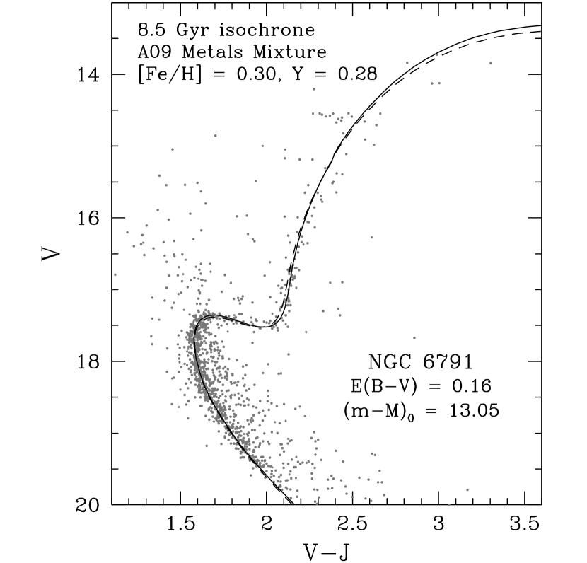
Figure 10: Using the reddening-corrected transformations given by Casagrande & VandenBerg (2014), an isochrone for the indicated age and chemical abundances (solid curve) has been overlaid onto $V\,J$ photometry of NGC 6791 (Brasseur et al. 2010). For reasons discussed in the text, the observed colors have been adjusted to the red by 0.04 mag. The dashed curve represents an 8.0 Gyr isochrone for $Y=0.30$ and the Grevesse & Sauval (1998) metal abundances, scaled to [Fe/H] $=+0.35$. Both isochrones were transposed to the observed plane assuming the reddening and true distance modulus specified in the lower right-hand corner.

Figure 10 shows that the observed RGB is redder (at $V\mathrel{\hbox{\raise 2.58334pt\hbox{$<$}\kern-7.74998pt\lower 2.15277pt\hbox{$\sim$}}}15.5$) than the isochrone which otherwise does a fine job of reproducing the fainter photometry. This suggests that either the model temperatures along the upper giant branch are too hot, or the adopted color–${T_{\rm eff}}$ relations for low gravities yield $V-J$ colors that are too blue, or both. As Brasseur et al. (2010) did not obtain $V\,J$ data for fainter MS stars than those plotted in Fig. 10, we are unable to comment on how well the isochrone fits near-IR data for LMS stars. However, the plots provided by Casagrande & VandenBerg (2014, see their Figs. 12 and 13) indicate that the same isochrone tends to deviate to the blue of the cluster MS at 2–3 mag below the turnoff (depending on the selected color index), while providing a comparable fit to the upper MS, TO, and SGB stars as that shown in Fig. 10. Presumably, the discrepancies at faint magnitudes are also indicative of errors in the model ${T_{\rm eff}}$ scale and/or the color transformations for cool, super-metal-rich stars.

The dashed curve in this figure represents an isochrone for 8.0 Gyr, $Y=0.30$, and [Fe/H] $=+0.35$ that has been computed assuming the $m$/Fe number abundance ratios given by Grevesse & Sauval (1998) instead of those determined by Asplund et al. (2009). As mentioned in the first paragraph of this section, Brogaard et al. (2012) derived a slightly higher age (8.3 Gyr) on the assumption of exactly the same chemical abundances. This is, however, the expected consequence of their adoption of a smaller value of $(m-M)_{V}$ by 0.04 mag, which is easily within the $1\,\sigma$ uncertainty associated with the cluster distance modulus (see the Brogaard et al. paper for a discussion of this issue). Fig. 10 shows that, with just a small difference in age, and minor changes to the adopted values of [Fe/H] and $Y$, isochrones based on either of the Grevesse & Sauval (1998) or Asplund et al. (2009) metals mixtures provide equally good fits to the CMD of NGC 6791 (as well as its binaries, see below). This reinforces the conclusions reached by Brogaard et al. from a similar analysis that such comparisons between theory and observations are not able to provide a clear preference for either solar abundance mixture, due in part to the compensating effects of the respective solar calibration.

The masses and radii that were determined for the components of the binaries V18 and V20 in NGC 6791 by Brogaard et al. (2012) are shown in Figure 11, along with the predicted MR relations from four different isochrones that assume scaled Asplund et al. (2009) metal abundances and one isochrone which assumes the same $m$/Fe ratios that were derived for the Sun by Grevesse & Sauval (1998). The solid and dashed curves represent the same isochrones that were plotted in the previous figure, and both provide reasonably good fits to the data. Indeed, very similar plots are given by Brogaard et al., who showed that it is only when $3\,\sigma$ error boxes are plotted that the observations can be intersected by a single isochrone. At this stage, it is not known whether the apparent discrepancies are due more to deficiencies in the models that have been compared with the observed masses and radii or to errors in the derived properties of the binaries. It would certainly be worthwhile to collect and analyze more observations of them and to add to the sample of completely eclipsing binaries that have been discovered to date in NGC 6791.

Be that as it may, Fig. 11 shows how the MR relation that is represented by the solid curve would be altered by, in turn, a 0.5 Gyr increase in age (the dot-dashed curve), a 0.05 dex reduction in [Fe/H] (the dotted curve), and a change in $Y$ by $+0.01$ (the long-dashed curve). According to these results, we would have obtained a closer match of the dashed locus to the solid curve, with an equally good fit to the cluster CMD, if the former assumed [Fe/H] $=+0.34$ (instead of $+0.35$) or a larger helium abundance by $\delta\,Y\approx 0.002$. (The effects of variations in [$\alpha$/Fe] have not been considered because, to within the uncertainties, the abundances of the $\alpha$ elements appear to be consistent with scaled solar values; see Brogaard et al. 2011.)

To conclude: aside from a possible zero-point error in the near-infrared photometry that we have used (Brasseur et al. 2010) or in the Casagrande & VandenBerg (2014) transformations to the $J$-band, our isochrones for [Fe/H] $\sim 0.3$ are able to reproduce the observed [$(V-J),\,V)$]-diagram of NGC 6791 quite well in a systematic sense — at least at $V-J\mathrel{\hbox{\raise 2.58334pt\hbox{$<$}\kern-7.74998pt\lower 2.15277pt\hbox{$\sim$}}}2.2$, which corresponds to ${T_{\rm eff}}\mathrel{\hbox{\raise 2.58334pt\hbox{$>$}\kern-7.3194pt\lower 2.15277pt\hbox{$\sim$}}}4600$ K. (Especially encouraging comparisons between the same isochrones and many other CMDs of this open cluster, derived from available $BVI$ and $ugriz$ photometry, are provided by Casagrande & VandenBerg.) We have also demonstrated that it is easy to use the models presented in this study to iterate on the age and chemical abundance parameters until a consistent fit is found to both an observed CMD and the MR relation that can be obtained from observations of detached, eclipsing binaries that belong to the same cluster.

5.3 Local Subdwarfs With $-2\mathrel{\hbox{\raise 2.58334pt\hbox{$<$}\kern-7.74998pt\lower 2.15277pt\hbox{$\sim$}}}$ [Fe/H] $\mathrel{\hbox{\raise 2.58334pt\hbox{$<$}\kern-7.74998pt\lower 2.15277pt\hbox{$\sim$}}}-1$

VandenBerg et al. (2010) have already shown that current Victoria-Regina stellar models satisfy the constraints provided by subdwarfs in the solar neighborhood that have well-determined $M_{V}$ values from Hipparcos. In fact, good consistency between theory and observations is obtained on several different color-magnitude planes, particularly those involving red or near-infrared colors (also see Brasseur et al. 2010), or on the $(\log{T_{\rm eff}},\,M_{V})$-diagram if the temperatures of the Population II dwarfs are obtained from Casagrande et al. (2010). The ${T_{\rm eff}}$ scale derived by the latter is $\sim 150$ K hotter than the one by Alonso, Arribas, & Martinez-Roger (1999, ), which was widely adopted during the last decade, though it agrees well with the hot temperature scale first proposed by King (1993), and three years later by Gratton, Carretta, & Castelli (1996). It may be recalled that the [Fe/H] values determined for GCs by Carretta & Gratton (1997) are based, in part, on a hot ${T_{\rm eff}}$ scale.

It is of some interest to revisit the work by R. G. Gratton and collaborators in the late 1990s, as their ${T_{\rm eff}}$ and [Fe/H] estimates for local subdwarfs are in remarkable agreement with the predictions of present-day isochrones. This is shown in Figure 12, which plots (in the bottom panel) the absolute visual magnitudes for the 10 subdwarfs with [Fe/H] $\mathrel{\hbox{\raise 2.58334pt\hbox{$<$}\kern-7.74998pt\lower 2.15277pt\hbox{$\sim$}}}-1.0$ that have the smallest values of $\sigma_{\pi}/\pi$ (van Leeuwen 2007), where $\pi$ represents the trigonometric parallax, as a function of their effective temperatures. The sources of the ${T_{\rm eff}}$ (and [Fe/H]) determinations are Gratton et al. (1996), Gratton et al. (1997), Clementini et al. (1999), and R. G. Gratton (2001, priv. comm., as reported by Bergbusch & VandenBerg 2001, see their § 4.1). If the models provided a perfect match to the observed stars, each of the subdwarfs would sit on the isochrone for its measured [Fe/H] value and the temperature implied by that isochrone would be identical to the spectroscopic estimate of ${T_{\rm eff}}$. (Of course, even the best metallicity and ${T_{\rm eff}}$ determinations are uncertain by $\sim\pm 0.2$ dex and $\sim\pm 70$ K, respectively. Furthermore, the ages of the subdwarfs could well be higher or lower than 12 Gyr — though most of them are sufficiently faint that the effect of the age uncertainty will have negligible consequences for our comparisons with the observations.)

The middle panel plots, as a function of the temperatures of the subdwarfs, the differences between the [Fe/H] values that were determined spectroscopically and those inferred from the isochrones that match the subdwarf locations in the $(\log{T_{\rm eff}},\,M_{V})$-diagram. For the sample of 10 stars, the mean offset is only 0.04 dex, in the sense that the observed iron abundances are just slightly less than the values deduced from the isochrones, with a standard deviation of 0.29 dex. Interestingly, the differences between the observed (“Obs”) and isochrone (“Iso”) metallicities tend to be $\mathrel{\hbox{\raise 2.58334pt\hbox{$>$}\kern-7.3194pt\lower 2.15277pt\hbox{$\sim$}}}0.0$ for stars that have [Fe/H] $\geq-1.5$ (those represented by open circles) whereas more metal-deficient stars, which are plotted as filled circles, all have “Obs $-$ Iso” values $<0.0$. However, there is no obvious variation of $\delta\,$[Fe/H] with temperature for either group of stars, which suggests that the models predict the correct lower-MS slopes.

One may alternatively interpolate in the isochrones to determine how much of an adjustment to the temperature of each subdwarf, at its observed $M_{V}$, would be required to locate it on the isochrone that has the same [Fe/H] as the subdwarf. The differences in ${T_{\rm eff}}$ so derived are plotted in the upper panel of Figure 12. Not surprisingly (because the abundance implied by a given line strength depends directly on the adopted temperature), stars with [Fe/H] $\geq-1.5$ tend to have “Obs $-$ Iso” values of $\delta\,{T_{\rm eff}}\mathrel{\hbox{\raise 2.58334pt\hbox{$>$}\kern-7.3194pt\lower 2.15277pt\hbox{$\sim$}}}0.0$, while the opposite is found for the most metal-poor stars. As in the middle panel, the level of agreement is surprisingly good: the mean offset and standard deviation are only $-11$ K and 65 K, respectively. Though the sample of stars is small, the models appear to fit the observations equally well over the entire temperature range encompassed by the stars. (Considering just the 10 subdwarfs in our sample, the temperatures and [Fe/H] values determined by R. G. Gratton and collaborators are, in the mean, 17 K and 0.09 dex higher, respectively, than the values tabulated by Casagrande et al. 2010.)

The same isochrones, when plotted on the [$(V-I)_{0},\,M_{V}$]- and [$(V-K)_{0},\,M_{V}$]-diagrams, provide equally satisfactory fits to the same subdwarfs — as shown in Figure 13. The differences in the predicted colors, which are based on the MARCS color–${T_{\rm eff}}$ relations (Casagrande & VandenBerg 2014), are obviously in excellent agreement with those observed (from Casagrande et al. 2010) since, on both color planes, $<\delta$(color)$>\ =0.00$, with relatively little scatter about the horizontal dashed line. Moreover, the models appear to fit the brighter, bluer stars just as well as the reddest, faintest ones. It is important to appreciate that relatively high temperatures must be assumed for the subdwarfs in order for the MARCS transformations to yield the observed colors. Most broad-band colors (especially $V-I$ and $V-K$) are much more dependent on ${T_{\rm eff}}$ than on [Fe/H] (or on gravity, which will, in any case, be close to $\log\,g=4.5$ for the Population II dwarfs). That is, our isochrones are able to provide good fits to the observations only because they predict the particular ${T_{\rm eff}}$ scale that yields the observed colors when derived from the MARCS color–${T_{\rm eff}}$ relations. Similar success would not have been obtained had the latter predicted much redder or bluer colors at the same ${T_{\rm eff}}$ or if we had adopted a significantly cooler empirical ${T_{\rm eff}}$ scale (e.g., Alonso et al. 1999, 1996).

Despite the indications from the spectroscopic results described above, the recent calibration of the infra-red flux method (IRFM) by Casagrande et al. (2010), the predictions of our stellar evolutionary models, and the color–temperature relations implied by the latest MARCS model atmospheres in support of a hot ${T_{\rm eff}}$ scale, it is important to remember that current 1D model atmospheres play a central role in each of these avenues of research. Indeed, as discussed by Magic et al. (2013), the very different temperature structures produced by 3D model atmospheres, particularly at low $Z$, are bound to impact ${T_{\rm eff}}$ and [$m$/H] determinations, as well as color transformations and the boundary conditions employed by stellar models. Indeed, the importance of advancing our understanding of model atmospheres, which provide the interface between stellar interior models and observed stars and stellar populations, can hardly be understated.

5.4 The Globular Clusters 47 Tuc, M 3, M 5, and M 92

In their extensive survey of GC ages, VandenBerg et al. (2013) found that isochrones generally provided reasonably good fits to the Hubble Space Telescope ACS (Advanced Camera for Surveys) photometry obtained by Sarajedini et al. (2007) when the cluster distances were determined from fits of zero-age horizontal-branch (ZAHB) loci to the observed HB stars. All of the models used in that investigation assumed the solar metal abundances given by Grevesse & Sauval (1998), with suitable enhancements to the abundances of $\alpha$-elements and then scaled to the [Fe/H] values derived by Carretta et al. (2009a). As we have not yet computed ZAHBs for the chemical mixtures assumed in this study, we are unable to follow exactly the same procedure here in order to ascertain, in particular, how the inferred distance moduli will differ from those found by VandenBerg et al. However, the predicted ZAHB luminosities, at the same [Fe/H], are likely to be quite similar because the main difference in the solar mixtures given by Grevesse & Sauval and Asplund et al. (2009) are the abundances of CNO, which mainly affect the color of the HB.

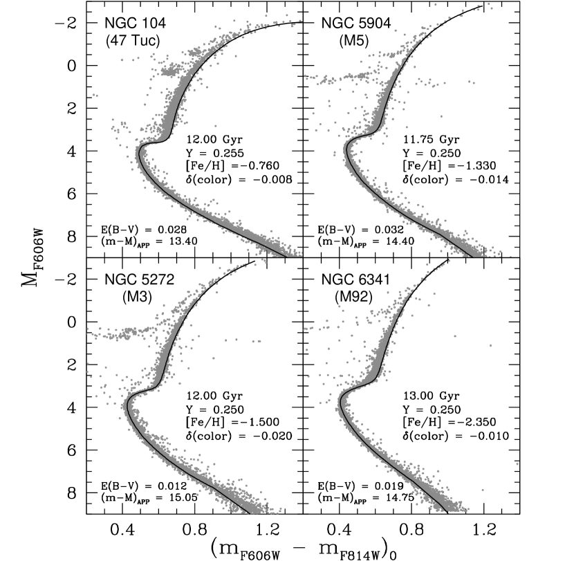
Figure 14: Fits of isochrones for the indicated ages and chemical abundances to the CMDs of 47 Tuc, M 3, M 5, and M 92 after the latter have been adjusted in the vertical and horizontal directions by the indicated distance moduli and reddenings (from the SF11 dust maps, and assuming $E(m_{F606W}-m_{F814W})=0.997\,E(B-V)$; Casagrande & VandenBerg 2014), respectively. In order for the selected isochrones to match the intrinsic turnoff colors, the model loci had to be corrected by the $\delta$(color) amounts specified in each panel. The source of the cluster photometry is Sarajedini et al. (2007).

Because TO luminosity versus age relations depend sensitively on the absolute abundance of oxygen (see V12), and because our models assume a smaller value of [O/Fe] (by 0.1 dex) as well as a lower solar abundance of oxygen, it can be expected that we will obtain higher ages for metal-poor clusters than those derived by VandenBerg et al. (2013) (if all other variables are kept constant). However, this is a moot point for the present discussion. Our main motivation for examining the CMDs of a few GCs is to check how well our models are able to reproduce the observed MS and RGB morphologies. To partially compensate for the expected effects of the different abundances of oxygen noted above (and of other metals), we have arbitrarily assumed slightly larger distance moduli (by $\mathrel{\hbox{\raise 2.58334pt\hbox{$<$}\kern-7.74998pt\lower 2.15277pt\hbox{$\sim$}}}0.05$ mag) and ages (by 0.25 Gyr) than the values derived by VandenBerg et al., and then matched the predicted and observed turnoffs. To accomplish this, it was necessary to apply a small blueward shift to the isochrones (by $\mathrel{\hbox{\raise 2.58334pt\hbox{$<$}\kern-7.74998pt\lower 2.15277pt\hbox{$\sim$}}}0.02$ mag) after the observed colors had been dereddened. The result of this exercise is shown in Figure 14 for the GCs 47 Tuc, M 3, M 5, and M 92. As in the VandenBerg et al study, the [Fe/H] values derived by Carretta et al. (2009a) have been assumed.

Except at $M_{F606W}\mathrel{\hbox{\raise 2.58334pt\hbox{$>$}\kern-7.3194pt\lower 2.15277pt\hbox{$\sim$}}}8$, where the solid curves deviate to the blue side of the observed lower-MS stars, the isochrones do quite a good job of matching the main sequences of the GCs over the entire range in [Fe/H] sampled by them. The biggest differences between theory and observations occur along the lower RGB, where the models are too red. However, the tendency of photometric scatter due to blending to be preferentially blueward on the giant branch may explain some fraction of such offsets (see Bergbusch & Stetson 2009). Curiously, the discrepancies resemble the effect on the location of the RGB of varying the helium content: as shown in Fig. 7, increasing $Y$ causes a larger temperature shift at the base of the giant branch than near the tip. On the other hand, it is possible that our treatment of the atmospheric boundary condition is responsible for the apparent difficulties (recall Fig. 4), or perhaps they signal some problems with the color–${T_{\rm eff}}$ relations that we have used or our treatment of convection. As noted in the introductory remarks given at the beginning of § 5, predicted temperatures and colors are subject to many uncertainties, and it should not be a surprise to find some discrepancies between isochrones and observed CMDs.

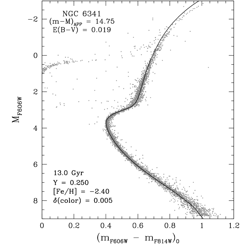
Figure 15: As in the bottom right-hand panel of the previous figure, except that the tracks on which the isochrones are based were obtained by matching MARCS model atmospheres to the interior structures at $\tau=100$ and the pressure at that depth was increased by $\delta\log P=+0.042$ (see Fig. 4). Note that a slightly lower [Fe/H] values was assumed in the one set of models that was computed for this case and that a small redward correction was applied to the isochrone colors in order to provide the best fit to the cluster MS stars.

To corroborate this point, we have generated isochrones for the case represented in Fig. 4 by the dot-dashed curve. That is, a full set of evolutionary tracks has been computed for [Fe/H] $=-2.40$, $Y=0.25$, and [$\alpha$/Fe] $=0.4$ in which the surface boundary conditions have been derived from the properties of MARCS model atmospheres at $\tau=100$, with the small increase in the pressure at that point implied by the corresponding Standard Solar Model. As shown in Figure 15, the 13 Gyr isochrone derived from these tracks, unlike the one plotted in the bottom, right-hand panel of the previous figure, provides a good fit to the lower RGB stars of M 92, but not those at higher luminosities. (Granted, the predicted turnoff is slightly too blue, but an improved fit to the TO could be obtained, without affecting the location of the lower RGB, simply by assuming a somewhat higher oxygen abundance.) In this example, the discrepancies along the upper giant branch could be telling us that, e.g., our treatment of convection or the adopted color–${T_{\rm eff}}$ relations are inadequate. We could force the models to provide an essentially perfect match to the data (by, for instance, suitable adjustments of the color transformations or the atmospheric boundary conditions), but the assumed distance and chemical abundances of M 92 may not be correct. Although isochrones may need to be “calibrated” for some investigations, not doing so enables one to retain the predictive power of stellar models. In fact, it is remarkable that current stellar models perform as well as they (appear to) do.

6 Summary

To obtain the correct understanding of stars and stellar populations, it is important to determine the observed chemical abundances and, in the case of complex systems (e.g., $\omega\,$Cen), their variations from star-to-star with as much accuracy and detail as possible through spectroscopic and photometric studies. It is just as important to interpret such data using stellar models for the observed chemistries because the most abundant metals (and helium) affect the predicted luminosities and temperatures of stars in different ways (see, e.g., V12). For this investigation, 126 grids of evolutionary tracks have been computed for, in each case, masses from $0.12{\cal M_{\odot}}$ to a sufficiently high mass that isochrones may be generated, using the accompanying software, for ages $\mathrel{\hbox{\raise 2.58334pt\hbox{$>$}\kern-7.3194pt\lower 2.15277pt\hbox{$\sim$}}}5$ Gyr, and arbitrary values of [Fe/H], $Y$, and [$\alpha$/Fe] within the ranges $-2.4\mathrel{\hbox{\raise 2.58334pt\hbox{$<$}\kern-7.74998pt\lower 2.15277pt\hbox{$\sim$}}}$ [Fe/H] $\mathrel{\hbox{\raise 2.58334pt\hbox{$<$}\kern-7.74998pt\lower 2.15277pt\hbox{$\sim$}}}+0.6$, $0.25\leq Y\leq 0.33$, and $-0.4\mathrel{\hbox{\raise 2.58334pt\hbox{$<$}\kern-7.74998pt\lower 2.15277pt\hbox{$\sim$}}}$ [$\alpha$/Fe] $\mathrel{\hbox{\raise 2.58334pt\hbox{$<$}\kern-7.74998pt\lower 2.15277pt\hbox{$\sim$}}}+0.4$. Comparisons of these computations with the CMDs of M 67, NGC 6791, local field subdwarfs, and four GCs (47 Tuc, M 3, M 5, and M 92) provide encouraging support for the models.

One point worth additional emphasis is that our models (and the MARCS color–${T_{\rm eff}}$ relations) favor a relatively hot temperature scale for metal-poor stars. This is not a new result, as virtually the same thing was found by Bergbusch & VandenBerg (2001). Indeed, if anything, an even warmer ${T_{\rm eff}}$ scale would be implied by the use of current MARCS model atmospheres as boundary conditions (see Fig. 4). Hotter stellar models could be at least part of the explanation of the long-standing problem that isochrones applicable to GCs are generally found to be slightly too red when well-supported estimates of the cluster distances, reddenings, and chemical abundances are adopted (e.g., see VandenBerg 2000, VandenBerg et al. 2013, and our Fig. 14). The difficulty with this solution is that the same models appear to satisfy the subdwarf constraint without needing any zero-point adjustment to the predicted colors (see Fig. 13), though this could be a fortuitous result if errors in the some of the subdwarf properties are compensating for the effects of errors in other properties. It is also possible that the apparent inconsistencies occur because GC metallicities, as generally measured in bright giants, are not on the same scale as those for Population II dwarfs. In particular, perhaps the [Fe/H] values of GCs are $\sim 0.15$–0.3 dex lower than the majority of current estimates — a possibility that is supported by recent spectroscopic studies of M 92 (Roederer & Sneden 2011) and M 15 (Preston et al. 2006, Sobeck et al. 2011), as well as other findings (VandenBerg et al. 2014).

Because of the overwhelming importance of oxygen for TO luminosity versus age relations, the next paper in this series will provide extensive grids of evolutionary tracks in which [O/Fe] is included among the chemical abundance parameters that can be varied. Among other things, Paper II will compare predicted and observed luminosities of the RGB bump, which is known to be a strong function of the oxygen abundance (see, e.g., Rood & Crocker 1985). (Accurate determinations of $V_{\rm bump}$ for more than 70 GCs are provided by by Nataf et al. 2013.) Following that investigation, fully consistent ZAHB models will be presented for the grids reported here and in Paper II so that it will be possible to assess their implications for distance determinations and to interpret the observed colors of HB stars.

APPENDIX

All of the model grids that have been computed for this investigation may be obtained from the Canadian Advanced Network for Astronomical Research (CANFAR) web site, together with several computer programs (in FORTRAN) that permit the user to generate isochrones on the theoretical plane, to transpose the isochrones to many different CMDs using the recent Casagrande & VandenBerg (2014) transformations, and to calculate luminosity functions (LFs), isochrone population functions (IPFs), and more. The methods that we have developed over the years to facilitate comparisons of models produced by the Victoria stellar evolutionary code with observational data are well described in V12 and references therein. In that paper, we added the ability to interpolate within the canonical grids to create grids of tracks with arbitrary helium abundances, $Y$, and/or metallicities, [Fe/H], within the ranges $-3.0\leq$ [Fe/H] $\leq-0.6$ and $0.25\leq Y\leq 0.33$. In this paper, we add the ability to interpolate the models in a third chemical abundance parameter, either ${\rm[\alpha/Fe]}$ (the elements O, Ne, Mg, Si, S, Ar, Ca, and Ti as a group) or ${\rm[m_{i}/Fe]}$, where ${\rm m_{i}}$ refers to one of C, N, O, Ne, Na, Mg, Al, Si, Ca, or Ti. Although V12 used three-point interpolation for both abundance parameters that they considered, we opted to employ linear interpolation in $Y$ and [Fe/H] to make the scheme more robust (in the sense that the age-mass relations which are critical for the isochrone interpolations are guaranteed to remain monotonic) and more flexible to use. Since only two values of ${\rm[\alpha/Fe]}$ are represented at $\mbox{${\rm[Fe/H]}$}=-2.0$ and +0.6 in the current computations (see Fig. 5), we also decided to use linear interpolation for the third abundance parameter.

Appendix A Format of the Track Files

As presented to the user, the evolutionary sequences are contained in EEP (equivalent evolutionary phase) files which have been processed in such a way that track points with the same model number are equivalent in every track in every grid. Two caveats apply to this prescription. First, in grids that extend to masses lower than $0.4{\cal M_{\odot}}$, tracks with masses $\leq 0.4{\cal M_{\odot}}$ are listed for equally logarithmically spaced ages from the zero-age main sequence (ZAMS) point up to a maximum age of $\approx$ 30 Gyr. Second, for those grids that contain tracks in which core contraction manifests itself after core hydrogen exhaustion, the main sequence turnoff point EEP (MSTO) becomes degenerate with the blue hook EEP (BLHK) for those lower mass tracks in which the blue hook is not present. We do not explictly list these degenerate points: their presence (discussed below) is indicated by listing the primary EEPS in the header lines for each track.

The canonical EEP file names (with the extension *.eep) provide all the abundance information for the tracks contained within them: each one begins with a five character prefix that terminates with the underscore character followed by three abundance specifications, e.g., a0zz_p4y29m18.eep. In this example, a0 indicates the solar metals mixture (Asplund et al., 2009) and zz specifies the entire group of $\alpha$-elements: decoding the rest of the name from left to right, p4 implies $\mbox{${\rm[\alpha/Fe]}$}=+0.4$, y29 implies $Y=0.29$, and m18 implies $\mbox{${\rm[Fe/H]}$}=-1.8$. A grid of tracks interpolated to $\mbox{${\rm[\alpha/Fe]}$}=+0.2$, $Y=0.273$, and $\mbox{${\rm[Fe/H]}$}=-0.75$ would have a0zz_p2y273m075.xeep as its file name, where the extension .xeep distinguishes it from the canonical grids. Had the interpolation been to $\mbox{${\rm[\alpha/Fe]}$}=-0.2$, $Y=0.273$, and $\mbox{${\rm[Fe/H]}$}=+0.25$, the file name would have been a0zz_m2y273p025.xeep — that is, the signs of the $\alpha$-element and iron abundances are denoted by either p ($+$ve) or m ($-$ve).

For future reference with grids in which individual elements may be enhanced differently with respect to some basic ${\rm[\alpha/Fe]}$  abundance ratio, such grids will have file names like a4xO_p1y25p02. The prefix a4xO decodes as “a basic $\mbox{${\rm[\alpha/Fe]}$}=+0.4$ mixture with an extra degree of enhancement of the element oxygen”. Decoding the rest of the name, p1 means that oxygen has been incrementally enhanced by +0.1 dex (above the amount in the basic ${\rm[\alpha/Fe]}$ mixture) so that $\mbox{${\rm[O/Fe]}$}=+0.5$, and y25p02 means $Y=0.25$ and $\mbox{${\rm[Fe/H]}$}=+0.2$. When the symbol for an element consists of a single letter (like C, N, or O), that letter appears just before the underscore, and x is used as a place-holder; otherwise, the third and fourth characters of the file name give the two-letter symbol of the metal (e.g., Ne, Mg) in question.

The contents of a *.eep file are illustrated in Figure 16. The header lines at the beginning of the file are reasonably straightforward to interpret (note, in particular, that the assumed [$m$/Fe] values are explicitly given for the main metals of interest), but the header lines for individual tracks require some explanation. The columns labeled Match, D(age), and D(log Teff) are redundant: they list information about how the models for the MS and SGB phases, which were obtained by solving the Lagrangian form of the stellar structure equations, were matched (at the base of the RGB) to the models for the subsequent evolution to the tip of the giant branch. As described in detail by VandenBerg (1992), a non-Lagrangian technique like the one developed by Eggleton (1971) was used to follow RGB evolution very efficiently. The indicated age and ${T_{\rm eff}}$ offsets were applied to the original track files for the RGB phase in order to obtain continuity with the Lagrangian models.

The column labeled Zage lists the ZAMS age as we defined it in V12. Six evolutionary phase points are listed under Primary EEPs. The default setting for each EEP-point is 0, which should be interpreted to mean (except for the ZAMS) that that particular evolutionary phase does not occur, or has not been reached, in that particular track. The ZAMS EEP-point is listed as model 1 when the track is included in the full isochrone interpolation scheme. When listed as 0, it signals that an interpolation to the isochrone age is to be made directly within that track. (Generally this applies to tracks with masses $\leq 0.4{\cal M_{\odot}}$. Points on the isochrone between those corresponding to these track masses are obtained by spline interpolation.) If the track evolves sufficiently, the MSTO is listed at model 801, and if a blue hook occurs it is listed at model 921. In the absence of a BLHK EEP, as is the case for the $0.9{\cal M_{\odot}}$ track in the grid shown, the base of the red giant branch (BRGB) occurs at model 1421, the evolutionary pause on the giant branch (GBPS) at model 1621, and the tip of the giant branch (GBTP) at model 1921. When the BLHK is non-zero, as is the case for the tracks with masses $>0.9{\cal M_{\odot}}$, the BRGB occurs at model 1541, the GBPS at 1741, and the RGBT at 2041.

In this example, tracks with masses $>0.9{\cal M_{\odot}}$ have BLHK EEPs while those with masses $\leq 0.9{\cal M_{\odot}}$ do not. (A “nascent” BLHK EEP may be identified in some tracks to relax the interpolation scheme through the transition from lower mass tracks with radiative cores at central H exhaustion to those higher mass tracks with fully developed convective cores at the end of the MS phase; see Bergbusch & VandenBerg 2001.) Consequently, 120 denerate EEP points would be inserted between the MSTO and BRGB for the lower mass tracks that evolve at least as far as the BRGB so that, for example, the BRGB in the $0.9{\cal M_{\odot}}$ track would change from model 1421 to model 1541. The same approach works when interpolating grids of tracks to some set of target abundances.

The first four columns in the listing for each track give the model number, $\log L/L_{\sun}$, $\log T_{\rm eff}$, and the age in Gyr. Columns 5 and 6 are reserved for the surface helium and ${\rm[Fe/H]}$ abundances (not implemented for the example shown in Fig. 16, while columns 7 and 8 list the derivatives of luminosity and of effective temperature with respect to time. The latter are needed for the calculation of LFs and IPFs.

Appendix B Interpolation Software

The interpolation of isochrones, LFs, and/or IPFs is made easy by the (FORTRAN) programs PBISO and PBIPF, which are improved versions of the MKISO and MKIPF codes, respectively, that were presented in previous publications (see V12 and references therein). We have now developed a new program, PBMIX, that can be used to interpolate within the canonical grids to produce a new grid of tracks at some set of the (up to) three abundance parameters — either (${\rm[\alpha/Fe]}$, $Y$, ${\rm[Fe/H]}$) or (${\rm[m_{i}/Fe]}$, $Y$, ${\rm[Fe/H]}$) that is signaled by the file name prefix. PBMIX makes use of a parameter file, PBMIX.PAR, that resides in the working directory; it contains a listing of the track masses employed in constructing the grid, the abundance ranges spanned by the grids, and a listing of all the EEP files encompassed by the abundance ranges specified. If PBMIX is run in a directory that doesn’t contain a PBMIX.PAR file, it will prompt you for all the requisite information and construct one automatically.

A sample file is shown in Figure 17. The first line lists the prefix for the file names associated with the grids contained in the working directory. (In this example, the grids have a basic $\mbox{${\rm[\alpha/Fe]}$}=+0.4$ mixture with additional enhancements to ${\rm[O/Fe]}$.) The next line begins with the number of tracks that may be associated with each grid, followed by the mass values — since the masses are read in via a list-directed read statement, they need only be separated by blanks and can be spread over several lines (two lines in this example). The (fourth) line following the list of masses gives the number of and canonical values for the abundance ratio ${\rm[O/Fe]}$. (If the file prefix were a0zz, this line would list the ${\rm[\alpha/Fe]}$ values instead.) The next (fifth) line does the same thing for the helium abundances, as does the (sixth) line for ${\rm[Fe/H]}$. Subsequently, the twenty-four canonical file names derived from the file prefix and the tabulated abundances — each with a unique set of ${\rm[O/Fe]}$, $Y$, and ${\rm[Fe/H]}$ — are listed.

Running PBMIX is very simple. When PBMIX.PAR already exists, the program simply prompts the user for the target ${\rm[\alpha/Fe]}$ value or the $\Delta\mbox{${\rm[m_{i}/Fe]}$}$ increment, and the target $Y$ and ${\rm[Fe/H]}$ values, then it creates the default output file name based on those targets and writes the interpolated tracks to that file. As in the case of the canonical grids, isochrones may be generated for the interpolated grids for any age in the range from $\sim 5$ Gyr to $\sim 15$ Gyr by executing PBISO. The auxilliary code PBIPF may then be used to provide magnitudes and colors in the Johnson-Cousins, 2MASS, Sloan, or Hubble Space Telescope ACS or WFC3 photometric systems. (The color transformation tables that are needed to accomplish this must be generated using the computer programs and data provided by Casagrande & VandenBerg 2014.) The same code provides the option of producing LFs or IPFs. A brief, but quite thorough, description of how to use each code is provided in a manual that can also be retrieved from the CANFAR web site.

Appendix C Tests of the Interpolation Software

To demonstrate that the interpolation errors are small, even though linear interpolation is employed for all three chemical abundance parameters, we have computed a set of evolutionary tracks for values of [Fe/H] $=-0.1$, [$\alpha$/Fe] $=+0.2$, and $Y=0.27$ that are midway between their respective grid values. These particular abundances were chosen because they lie along the [$\alpha$/Fe] versus [Fe/H] relationship that has been derived for stars in the Galactic Bulge (e.g., Ryde et al. 2010, their Fig. 3), where the “knee” in that relation, which is believed to represent the point at which Type Ia supernovae began to contribute to the chemical evolution of the Bulge, occurs at an unusually high [Fe/H] value ($\approx-0.3$). (To produce this grid, the necessary opacity data were generated in the usual way; see § 3.) It can be expected that this case will provide quite a severe test of the interpolation scheme because (i) the difference between a line that connects any two of the points that are fitted by a parabolic curve, and that parabola, will be maximal at approximately the mid-point, and (ii) the effects of opacity on mass-luminosity and age-mass relations are strongest at the highest metal abundances.

However, as shown in Figure 18, isochrones derived from this set of models differ only slightly from those for the same age that are obtained by interpolation in the grids which are being provided for general use via this paper. At a value of $\log\,{T_{\rm eff}}$ that is 0.01 dex cooler than the turnoff temperature, the subgiant branches of the interpolated isochrones are $\mathrel{\hbox{\raise 2.58334pt\hbox{$<$}\kern-7.74998pt\lower 2.15277pt\hbox{$\sim$}}}0.04$ mag brighter than the SGBs of isochrones that have been derived from evolutionary tracks computed for the same values of $Y$, [$\alpha$/Fe], and [Fe/H]. This is not negligible, but as noted above, the interpolation errors are expected to be larger for this case than for most other choices of the abundance parameters that are representative of the observed abundances in stars. For instance, the transition from [$\alpha$/Fe] $\approx+0.4$ to 0.0 typically begins at [Fe/H] $<-1.0$ in dwarf galaxies (Venn et al. 2004), and the second test case that we have considered (for $Y=0.26$, [$\alpha$/Fe] $=+0.2$, and [Fe/H] $=-0.9$) shows that the computed and interpolated isochrones which are applicable to such systems will be indistinguishable (see Fig. 18).

We would have preferred to compute grids of evolutionary sequences for $\delta$[$\alpha$/Fe] $=0.2$, but the model atmospheres that are needed to provide the surface boundary conditions for the lowest mass models are not currently available for such a fine spacing of this quantity. It turns out, in fact, that most of the interpolation errors at high metallicities occur because a grid spacing of 0.4 dex range in [$\alpha$/Fe] is too large. We reached this conclusion after comparing computed and interpolated isochrones for a third case; specifically, [$\alpha$/Fe] $=0.0$ (one of the grid values), $Y=0.27$, and [Fe/H] $=+0.30$, where the latter quantities are at the mid-points of the grid values, $Y=0.25$, 0.29 and [Fe/H] $=+0.2$, $+0.4$, respectively. To avoid making Fig. 8 too complicated, we elected not to plot these two isochrones, but we found that they superimpose each other so well that the differences between them are barely discernible.

V12 (see their Figs. 4–6) had previously demonstrated that the errors associated with $Y$, [Fe/H] interpolations are negligible if the grid spacings of these variables are $\delta\,Y=0.04$ and $\delta$[Fe/H] $=0.2$ dex. Although they used three-point interpolations in the tests that they conducted, we have found that linear interpolations work nearly as well (even at high metal abundances). Thus, there appears to be only a small regime of parameter space ([$\alpha$/Fe] roughly halfway between the grid values, but only at relatively high [Fe/H] values) where minor interpolation errors can be expected. Elsewhere, such errors are of no consequence whatsoever.

Figure 1: Plot on an H-R diagram of 0.10 to $0.50{\cal M_{\odot}}$ models (open circles) for [Fe/H] $=0.0$ and an age of 5 Gyr, on the assumption of three different treatments of the atmospheric layers. The dashed and solid curves connect the models that were obtained by fitting MARCS model atmospheres (Gustafsson et al. 2008) to the interior structures at the photosphere (the layer where $T={T_{\rm eff}}$) or at $\tau=100$, respectively. The scaled-solar, Holweger & Müller (1974) $T$–$\tau$ relation was used to derive the boundary pressure (see the text) in the case of the models that are connected by the dot-dashed curve. The small filled circles represent the lower-MS segment of a 4 Gyr, solar-metallicity isochrone provided by G. Feiden (2011, priv. comm.). PHOENIX model atmospheres (Hauschildt et al. 1999) were used to provide the boundary conditions for these models, with the fitting point chosen to be photosphere or $\tau=100$ for masses $>0.2{\cal M_{\odot}}$ or $\leq 0.2{\cal M_{\odot}}$, respectively.

Figure 2: Upper panels: Plot on the H-R diagram of cubic spline fits (solid curves) to the ZAMS locations (filled circles) of models for the indicated masses and helium abundances, assuming [$\alpha$/Fe] $=0.0$ and [Fe/H] values ranging from $-1.0$ to $+0.6$, in 0.2 dex increments (in the direction from left to right). At a given mass, the ZAMS models move along diagonal lines toward lower luminosities and cooler temperatures as the metallicity increases: note the progression of the filled curcles that represent each mass value. Lower panels: Plot of the same loci that are shown in the upper panels, except on the mass-luminosity plane.

Figure 3: Left-hand plot: the solid curves represent 10 Gyr isochrones for the indicated values of $Z$ (from our grids for [$\alpha$/Fe] $=0.4$ and $Y=0.25$), while the filled circles along them give the locations of 0.12, 0.15, 0.20, 0.25, 0.30, and $0.35{\cal M_{\odot}}$ models (in the direction from lower to higher luminosities). The open circles indicate the locations of models for the same $Z$, [$\alpha$/Fe], and masses (assuming $Y=0.245+1.6\,Z$) along isochrones (not shown) computed by Dotter et al. (2007b). (It is not known why the faintest open circle for $Z=0.004$ deviates so much from our model for the same mass and $Z$.) Right-hand plot: Comparison on the mass-radius plane of a 5 Gyr isochrone (solid curve) for the indicated values of $Y$ and [Fe/H] with the observed properties of the lowest mass components of the triple system KOI-126 (Carter et al. 2011, Feiden et al. 2011). The assumed value of $Y$ is just slightly larger than the value required by a Standard Solar Model ($Y=0.2553$). The short-dashed and long-dashed curves represent isochrones that are otherwise the same, except that they assume [Fe/H] $=+0.07$ and $=+0.23$, respectively, to illustrate the effects on the mass-radius diagram of varying the observed metallicity by $\pm 1\,\sigma$.

Figure 4: Evolutionary tracks for the indicated masses and chemical abundances, but for different treatments of the atmospheric boundary condition (see the text). As noted in the legend in the lower right-hand corner, the dotted curves indicate the tracks in which a scaled Holweger & Müller (1974) $T$–$\tau$ structure was assumed in determining the surface pressure, while the other loci were obtained as the result of attaching MARCS model atmospheres (Gustafsson et al. 2008) to the interior structures at the photosphere or at depth ($\tau=100$). In two of the latter cases, ad hoc corrections were applied to the predicted pressure at $T={T_{\rm eff}}$ (dP${}_{1}=\delta\log P=-0.130$) or at $\tau=100$ (dP${}_{2}=\delta\log P=+0.042$) in order for a $1{\cal M_{\odot}}$, solar abundance model to reproduce the luminosity and temperature of the Sun at the solar age.

Figure 5: Grids of evolutionary tracks for $Y=0.25,0.29,$ and 0.33 have been computed for the values of [Fe/H] and [$\alpha$/Fe] which are designated by the open circles. The boxes defined by the dotted and dashed lines indicate the regions of parameter space that are used when interpolating for models that have $0.0\leq$ [$\alpha$/Fe] $\leq 0.4$ and $-0.4\leq$ [$\alpha$/Fe] $<0.0$, respectively (see the Appendix). The solid curve represents one of many possible relations between [$\alpha$/Fe] and [Fe/H] that may be assumed when modelling a particular stellar population.

Figure 6: Plot on an H-R diagram of 11 Gyr isochrones for the indicated helium and $\alpha$-element abundances, on the assumption of [Fe/H] values that vary from $-2.4$ to $+0.4$ (in the direction from left to right), in 0.2 dex increments.

Figure 7: Comparison of three of the isochrones from the previous figure (i.e., for $Y=0.25$, [$\alpha$/Fe] $=0.4$ and [Fe/H] $=-2.0$, $-1.0$, and 0.0: solid curves) with isochrones which are otherwise identical, except that the assumed helium abundances are $Y=0.29$ (dotted curves) and $Y=0.33$ (dashed curves).

Figure 8: Similar to the previous figure, except that the dependence of 11 Gyr isochrones for $Y=0.25$ and [Fe/H] $=-2.0$, $-1.0$, and 0.0 on [$\alpha$/Fe] is shown. As indicated, the solid, dotted, and dashed curves assume [$\alpha$/Fe] $=+0.4$, 0.0, and $-0.4$, respectively.

Figure 9: Overlay of a 4.3 Gyr isochrone for the indicated values of [Fe/H] and $Y$ onto the CMD of M 67 (see Brasseur et al. 2010) on the assumption of $E(B-V)=0.03$ (from SF11), $E(V-K_{S})=2.76\,E(B-V)$ (Casagrande & VandenBerg 2014) and an apparent distance modulus $(m-M)_{V}=9.69$. The solar symbol (at $V-K=1.56$, $M_{V}=4.82$) indicates the location of the Sun on this diagram. The main point of this plot is that the observed MS and RGB are matched quite well by the models in both an absolute and systematic sense.

Figure 11: Comparison on the mass-radius plane of isochrones for the indicated values of $Y$, [Fe/H], and age with the properties of the binaries V18 and V20 in NGC 6791 (as represented by the small filled circles and the $1\,\sigma$ error rectangles). Numerical values for the latter are given by Brogaard et al. (2012, see their Table 1). The solid and dashed curves represent the same isochrones that were plotted in the previous figure.

Figure 12: Lower panel: superposition of those nearby subdwarfs with [Fe/H] $\mathrel{\hbox{\raise 2.58334pt\hbox{$<$}\kern-7.74998pt\lower 2.15277pt\hbox{$\sim$}}}-1.0$ that have the most precise $M_{V}$ values (from Hipparcos) onto 12 Gyr isochrones for the indicated [Fe/H] values (in 0.2 dex increments). Open circles denote subdwarfs with [Fe/H] $\geq-1.5$, whereas the stars with lower metallicities have been plotted as filled circles. The stars are identified by their HD numbers. See the text for the sources of their ${T_{\rm eff}}$ and [Fe/H] values. Middle panel: the difference between the observed [Fe/H] value and that inferred for each star from the interpolated (or extrapolated) isochrone that matches its location in the bottom panel. Upper panel: the shift in ${T_{\rm eff}}$ that would have to be applied to each subdwarf in order for it to be located on the isochrone (in the bottom panel) for its observed [Fe/H] value. The arrows and adjacent numbers in the middle and upper panels indicate the mean values of $\delta\,$[Fe/H] and $\delta{T_{\rm eff}}$, respectively, along with the standard deviations (in parentheses) for the subdwarf samples in the sense “observed minus predicted”.

Figure 13: Similar to the previous figure, except that the properties of the same subdwarfs are compared with isochrones that have been transposed to the $V-I$ and $V-K$ color planes using the MARCS color–${T_{\rm eff}}$ relations reported by Casagrande & VandenBerg (2014). The observed colors are from the study by Casagrande et al. (2010).

Figure 16: Header lines and entries for selected tracks in the file a0zz_ p4y25m02.eep. Listings of the primary EEPs for each track provide the information needed to connect the secondary EEPs between tracks of different masses within a grid for isochrone interpolation, and between tracks with identical masses in different grids for track interpolation.

Figure 17: A sample PBMIX.PAR file for a set of twenty-four canonical grids containing up to twelve tracks with masses ranging from 0.4 to $1.5{\cal M_{\odot}}$, constructed with a basic $\mbox{${\rm[\alpha/Fe]}$}=+0.4$ mixture at combinations of $\mbox{${\rm[O/Fe]}$}[+0.2,+0.4,+0.6]$, $Y[0.245,0.285]$, and $\mbox{${\rm[Fe/H]}$}[-2.0,-2.2,-2.4,-2.6]$.

Figure 18: Comparisons of 7.0 and 12.0 Gyr isochrones for the indicated values of $Y$, [Fe/H], and [$\alpha$/Fe]. The dashed curves were obtained by interpolating in the grids of models that are presented in this paper. The solid curves are based on grids of evolutionary tracks that were computed for the specified abundances, and thus do not involve any interpolations whatsoever of the chemical abundance parameters.

Table 1: Adopted ($\log\,N$) Metal Abundances

Element	[$\alpha$/Fe] $=0.0$ Mix	[$\alpha$/Fe] $=-0.4$ Mix	[$\alpha$/Fe] $=+0.4$ Mix
Cstring	8.43	8.43	8.43
Nstring	7.83	7.83	7.83
Ostring	8.69	8.29	9.09
Nestring	7.93	7.53	8.33
Nastring	6.24	6.24	6.24
Mgstring	7.60	7.20	8.00
Alstring	6.45	6.45	6.45
Sistring	7.51	7.11	7.91
Pstring	5.41	5.41	5.41
Sstring	7.12	6.72	7.52
Clstring	5.50	5.50	5.50
Arstring	6.40	6.00	6.80
Kstring	5.03	5.03	5.03
Castring	6.34	5.94	6.74
Tistring	4.95	4.55	5.35
Crstring	5.64	5.64	5.64
Mnstring	5.43	5.43	5.43
Festring	7.50	7.50	7.50
Nistring	6.22	6.22	6.22

References

- (1) Alonso, A., Arribas, S., & Martinez-Roger, C. 1996, A&AS, 117, 227
- Alonso, Arribas, & Martinez-Roger (1999) Alonso, A., Arribas, S., & Martinez-Roger, C. 1999, A&AS, 140, 261
- Asplund, Grevesse, & Sauval (2005) Asplund, M., Grevesse, N., & Sauval, A. J. 2005, in ASP Conf. Ser. 336, Cosmic Abundances as Records of Stellar Evolution and Nucleosynthesis, eds. T. G. Barnes, III & F. N. Bash (San Francisco, CA: ASP), 25
- Asplund et al. (2009) Asplund, M., Grevesse, N., Sauval, A. J., & Scott, P. 2009, ARA&A, 47, 481
- Bergbusch & Stetson (2009) Bergbusch, P. A., & Stetson, P. B. 2009, AJ, 138, 1455
- Bergbusch & VandenBerg (1992) Bergbusch, P. A., & VandenBerg, D. A. 1992, ApJS, 81, 163
- Bergbusch & VandenBerg (2001) Bergbusch, P. A., & VandenBerg, D. A. 2001, ApJ, 556, 322
- Boesgaard, Jensen, & Deliyannis (2009) Boesgaard, A. M., Jensen, E. E. C., & Deliyannis, C. P. 2009, AJ, 137, 4949
- Brasseur et al. (2010) Brasseur, C. M., Stetson, P. B., VandenBerg, D. A., Casagrande, L., Bono, G., & Dall’Ora, M. 2010, AJ, 140, 1672
- Bressan et al. (2012) Bressan, A., Marigo, P., Girardi, L., et al. 2012, MNRAS, 427, 127
- Brocato, Cassisi, & Castellani (1998) Brocato, E., Cassisi, S., & Castellani, V. 1998, MNRAS, 295, 711
- Brogaard et al. (2011) Brogaard, K., Bruntt, H., Grundahl, F., Clausen, J. V., Frandsen, S., VandenBerg, D. A., & Bedin, L. R. 2011, A&A, 525, A2
- Brogaard et al. (2012) Brogaard, K., VandenBerg, D. A., Bruntt, H., et al. 2012, A&A, 543, A106
- Carney (1981) Carney, B. W. 1981, in IAU Colloq. No. 68, Astrophysical Parameters for Globular Clusters, ed. A. G. D. Philip & D. S. Hayes (Schenectady, NY: L. Davis Press), 477
- Carretta et al. (2009a) Carretta, E., Bragaglia, A., Gratton, R. G., D’Orazi, V., & Lucatello, S. 2009a, A&A, 508, 695
- Carretta et al. (2009b) Carretta, E., Bragaglia, A., Gratton, R. G., & Lucatello, S. 2009b, A&A, 505, 139
- Carretta et al. (2010) Carretta, E., Bragaglia, A., Gratton, R. G., et al. 2010, A&A, 516, 55
- Carretta & Gratton (1997) Carretta, E., & Gratton, R. G. 1997, A&AS, 121, 95
- Carter et al. (2011) Carter, J. A., Fabrycky, D. C., Ragozzine, D., et al. 2011, Science, 331, 562
- Casagrande et al. (2012) Casagrande, L., Ramírez, I., Meléndez, J., & Asplund, M. 2012, ApJ 761, 16
- Casagrande et al. (2010) Casagrande, L., Ramírez, I., Meléndez, J., Bessell, M., & Asplund, M. 2010, A&A, 512, 54.
- Casagrande & VandenBerg (2014) Casagrande, L., & VandenBerg, D. A. 2014, MNRAS, in press, arXiv: 1407.6095
- (23) Cassisi, S., Mucciarelli, A., Pietrinferni, A., Salaris, M., & Ferguson, J.W. 2013, A&A, 554, A19
- Cassisi et al. (2008) Cassisi, S., Salaris, M., Pietrinferni, A., et al. 2008, ApJ, 672, 275
- Castellani et al. (1997) Castellani, V., Ciacio,F., Degl’Innocenti, S., & Fiorentini, G. 1997, A&A, 322, 801
- Clementini et al. (1999) Clementini, G., Gratton, R. G., Carretta, E., & Sneden, C. 1999, MNRAS, 302, 22
- Cohen (2004) Cohen, J. G. 2004, AJ, 127, 1545
- Dalessandro et al. (2013) Dalessandro, E., Salaris, M., Ferraro, F. R., Mucciarelli, A., & Cassisi, S. 2013, MNRAS, 430, 459
- Dell’Omodarme et al. (2012) Dell’Omodarme, M., Valle, G., Degl’Innocenti, S., & Prada Moroni, P. G. 2012, A&A, 540, A26
- Dinescu et al. (2000) Dinescu, D. I., Majewski, S. R., Girard, T. M., & Cudworth, K. M. 2000, AJ, 120, 1892
- Dotter et al. (2007a) Dotter, A., Chaboyer, B., Ferguson, J. W., et al. 2007a, ApJ, 666, 403
- Dotter et al. (2007b) Dotter, A., Chaboyer, B., Jevremović, D., et al. 2007b, AJ, 134, 376.
- Eggleton (1971) Eggleton, P. P. 1971, MNRAS, 151, 351
- Fabbian et al. (2009) Fabbian, D., Nissen, P. E., Asplund, M., Pettini, M., & Ackerman, C. 2009, A&A, 500, 1143
- Feiden & Chaboyer (2013) Feiden, G. A., & Chaboyer, B. 2013, ApJ, 779, 183
- Feiden, Chaboyer, & Dotter (2011) Feiden, G. A., Chaboyer, B., & Dotter, A. 2011, ApJL, 740, L25
- Ferguson et al. (2005) Ferguson, J. W., Alexander, D. R., Allard, F., et al. 2005, ApJ, 623, 585
- Ferguson & Dotter (2008) Ferguson, J. W., & Dotter, A. 2008, IAU Symp. 252, The Art of Making Stars in the 21st Century, eds. L. Deng, K. L. Chan, & C. Chiosi (Cambridge: Cambridge Univ. Press), p. 1
- Ferraro et al. (2006) Ferraro, F. R., Valenti, E., Straniero, O., & Livia, O. 2006, ApJ, 642, 225
- Garnavich et al. (1994) Garnavich, P. M., VandenBerg, D. A., Zurek, D., & Hesser, J. E. 1994, AJ, 107, 1097
- Gratton et al. (2001) Gratton, R. G., Bonifacio, P., Bragaglia, A., et al. 2001, A&A, 369, 87
- Gratton, Carretta, & Bragaglia (2012) Gratton, R. G., Carretta, E., & Bragaglia, A. 2012, A&AR, 20, 50
- Gratton, Carretta, & Castelli (1996) Gratton, R. G., Carretta, E., & Castelli, F. 1996, A&A, 314, 191
- Gratton et al. (1997) Gratton, R. G., Fusi Pecci, F., Carretta, E., Clementini, G., Corsi, C. E., & Lattanzi, M. 1997, ApJ, 491, 749
- Gratton et al. (2013) Gratton, R. G., Lucatello, S., Sollima, A., et al. 2013, A&A, 549, A41
- Grevesse & Sauval (1998) Grevesse, N., & Sauval, A. J. 1998, Space Sci. Rev., 85, 161
- Gruyters et al. (2013) Gruyters, P., Korn, A. J., Richard, O., et al. 2013, A&A, 555, A31
- Gustafsson et al. (2008) Gustafsson, B., Edvardsson, B., Eriksson, K., et al. 2008, A&A, 486, 951
- Hauschildt et al. (1999) Hauschildt, P. H., Allard, F., Ferguson, J., Baron, E., & Alexander, D. R. 1999, ApJ, 525, 871
- Holweger & Müller (1974) Holweger, H., & Müller, E. A. 1974, Sol. Phys., 39, 19 (HM74)
- Iglesias & Rogers (1996) Iglesias, C. A., & Rogers, F. J. 1996, ApJ, 464, 943
- King (1993) King, J. 1993, AJ, 106, 1206
- Korn et al. (2007) Korn, A. J., Grundahl, F., Richard, O., et al. 2007, ApJ, 670, 774
- Johnson & Pilachowski (2010) Johnson, C. I., & Pilachowski, C. A. 2010, ApJ, 722, 1373
- Lecureur et al. (2007) Lecureur, A., Hill, V., Zoccali, M., et al. 2007, A&A, 465, 799
- Magic et al. (2013) Magic, Z., Collet, R., Asplund, M., et al. 2013, A&A, 557, A26
- Marino et al. (2008) Marino, A. F., Villanova, S., Piotto, et al. 2008, A&A, 625, 640
- Marino et al. (2009) Marino, A. F., Milone, A. P., Piotto, G., et al. 2009, A&A, 505, 1099
- Michaud et al. (2004) Michaud, G., Richard, O., Richer, J., & VandenBerg, D. A. 2004, ApJ, 606, 452
- Michaud, Richer, & Richard (2010) Michaud, G., Richer, J., & Richard, O. 2010, A&A, 510, A104.
- Morel et al. (1994) Morel, P., van’t Veer, C., Provost, J., et al. 1994, A&A, 286, 91
- Nataf et al. (2013) Nataf, D. M., Gould, A., Pinsonneault, M. H., & Udalski, A. 2013, ApJ, 766, 77
- Önehag, Gustafsson, & Korn (2014) Önehag, A., Gustafsson, B., & Korn, A. 2014, A&A, in press
- Önehag et al. (2011) Önehag, A., Korn, A., Gustafsson, B., Stempels, E., & VandenBerg, D. A. 2011, A&A, 528, A85
- Origlia et al. (2006) Origlia, L., Valenti, E., Rich, R. M., & Ferraro, F. 2006, ApJ, 646, 499
- Paust, Chaboyer, & Sarajedini (2007) Paust, N. E. Q., Chaboyer, B., & Sarajedini, A. 2007, AJ, 133, 2787
- Paxton et al. (2011) Paxton, B., Bildsten, L., Dotter, A., et al. ApJS, 192, 3
- Pereira et al. (2013) Pereira, T. M. D., Asplund, M., Collet, R., et al. 2013, A&A, 554, A118.
- Pietrinferni et al. (2006) Pietrinferni, A., Cassisi, S., Salaris, M., & Castelli, F. 2006, ApJ, 642, 797
- Piotto et al. (2007) Piotto, G., Bedin, L. R., Anderson, J., et al. 2007, ApJL, 661, L53
- Preston et al. (2006) Preston, G. W., Sneden, C., Thompson, I. B., Schectman, S. A., & Burley, G. S. 2006, AJ, 132, 85
- Proffitt & VandenBerg (1991) Proffitt, C. R., & VandenBerg, D. A. 1991, ApJS, 77, 473
- Ramírez, Meléndez, & Chanamé (2012) Ramírez, I., Meléndez, J., & Chanamé, J. 2012, ApJ, 575, 164
- Ramírez & Cohen (2002) Ramírez, I., & Cohen, J. 2002, AJ, 123, 3277
- Randich et al. (2006) Randich, S., Sestito, P., Primas, F., Pallavicini, R., & Pasquini, L. 2006, A&A, 450, 557
- Richard, Michaud, & Richer (2001) Richard, O., Michaud, G., & Richer, J. 2001, ApJ, 558, 377
- Richer et al. (2008) Richer, H. B., Dotter, A., Hurley, J., et al. 2008, AJ, 135, 2141
- Richer et al. (1998) Richer, H. B., Fahlman, G. G., Rosvick, J., & Ibata, R. 1998, ApJL, 504, L91
- Richer, Michaud, & Turcotte (2000) Richer, J., Michaud, G., & Turcotte, S. 2000, ApJ, 529, 338
- Roederer & Sneden (2011) Roederer, I. U., & Sneden, C. 2011, AJ, 142, 22
- Rood & Crocker (1985) Rood, R. T., & Crocker, D. A. 1985, Production and Distribution of C,N,O Abundances, eds. I. J. Danziger, F. Matteucci, & K. Kjär (Garching bei München: ESO), p. 61
- Ryde et al. (2010) Ryde, N., Gustafsson, B., Edvardsson, B., et al. 2010, A&A, 509, A20
- Salaris, Chieffi, & Straniero (1993) Salaris, M., Chieffi, A., & Straniero, O. 1993, ApJ, 414, 580
- Salaris et al. (2006) Salaris, M., Weiss, A., Ferguson, J. W., & Fusilier, D. J. 2006, ApJ, 645, 1131
- Sarajedini et al. (2007) Sarajedini, A., Bedin, L. R., Chaboyer, B., et al. 2007, AJ, 133, 1658
- Schlafy & Finkbeiner (2011) Schlafy, E. F., & Finkbeiner, D. P. 2011, ApJ, 737, 103 (SF11)
- Schlegel, Finkbeiner, & Davis (1998) Schlegel, D. J., Finkbeiner, D. P., & Davis, M. 1998, ApJ, 500, 525
- Skrutskie et al. (2006) Skrutskie, M. F., Cutri, R. M., Stiening, R., et al. 2006, AJ, 131, 1163
- Sobeck et al. (2011) Sobeck, J. S., Kraft, R. P., Sneden, C., et al. 2011, AJ, 141, 175
- Stetson (2005) Stetson, P. B. 2005, PASP, 117, 563
- Stetson, Bruntt, & Grundahl (2003) Stetson, P. B., Bruntt, H., & Grundahl, F. 2003, PASP, 115, 413
- Valcarce, Catelan, & Sweigart (2012) Valcarce, A. A. R., Catelan, M., & Sweigart, A. V. 2012, A&A, 547, A5
- VandenBerg (1992) VandenBerg, D. A. 1992, ApJ, 391, 685
- VandenBerg (2000) VandenBerg, D. A. 2000, ApJS, 129, 315
- VandenBerg et al. (2012) VandenBerg, D. A., Bergbusch, P. A., Dotter, A., et al. 2012, ApJ, 755, 15 (V12)
- VandenBerg, Bergbusch, & Dowler (2006) VandenBerg, D. A., Bergbusch, P. A., & Dowler, P. D. 2006, ApJS, 162, 375
- VandenBerg et al. (2014) VandenBerg, D. A., Bond, H. E., Nelan, E. P., Nissen, P. E., Schaefer, G. H., & Harmer, D. 2014, ApJ, in press, arXiv: 1407.7591
- VandenBerg et al. (2013) VandenBerg, D. A., Brogaard, K., Leaman, R., & Casagrande, L. 2013, ApJ, 775, 134
- VandenBerg, Casagrande, & Stetson (2010) VandenBerg, D. A., Casagrande, L., & Stetson, P. B. 2010, AJ, 140, 1020
- VandenBerg et al. (2008) VandenBerg, D. A., Edvardsson, B., Eriksson, K., & Gustafsson, B. 2008, ApJ, 675, 746
- VandenBerg et al. (2007) VandenBerg, D. A., Gustafsson, B., Edvardsson, B., Eriksson, K., & Ferguson, J. 2007, ApJL, 666, L105
- VandenBerg & Poll (1989) VandenBerg, D. A., & Poll, H. E. 1989, AJ, 98, 1451
- VandenBerg et al. (2000) VandenBerg, D. A., Swenson, F. J., Rogers, F. J., Iglesias, C. A., & Alexander, D. R. 2000, ApJ, 532, 430
- van Leeuwen (2007) van Leeuwen, F. 2007, A&A, 474, 653
- Venn et al. (2004) Venn, K. A., Irwin, M., Shetrone, M. D., Tout, C. A., Hill, V., & Tolstoy, E. 2004, AJ, 128, 1177
- Wapstra & Bos (1977) Wapstra, A. H., & Bos, K. 1977, Atom. Data and Nuc. Data Tab., 19, 177
_
p4y25m02.eep. Listings of the primary
EEPs for each track provide the information needed to connect the
secondary EEPs between tracks of different masses within a grid
for isochrone interpolation, and between tracks with identical
masses in different grids for track interpolation.