A Numerical Algorithm for
$L_{2}$ Semi-Discrete Optimal Transport in 3D

Abstract.

This paper introduces a numerical algorithm to compute the $L_{2}$ optimal transport map between two measures $\mu$ and $\nu$, where $\mu$ derives from a density $\rho$ defined as a piecewise linear function (supported by a tetrahedral mesh), and where $\nu$ is a sum of Dirac masses.

I first give an elementary presentation of some known results on optimal transport and then observe a relation with another problem (optimal sampling). This relation gives simple arguments to study the objective functions that characterize both problems.

I then propose a practical algorithm to compute the optimal transport map between a piecewise linear density and a sum of Dirac masses in 3D. In this semi-discrete setting, Aurenhammer et.al [8th Symposium on Computational Geometry conf. proc., ACM (1992)] showed that the optimal transport map is determined by the weights of a power diagram. The optimal weights are computed by minimizing a convex objective function with a quasi-Newton method. To evaluate the value and gradient of this objective function, I propose an efficient and robust algorithm, that computes at each iteration the intersection between a power diagram and the tetrahedral mesh that defines the measure $\mu$.

The numerical algorithm is experimented and evaluated on several datasets, with up to hundred thousands tetrahedra and one million Dirac masses.

Introduction

Optimal Transportation, initially studied by Monge [24], is a very general problem formulation that can be used as a model for a wide range of applications domains. In particular, it is a natural formulation for several fundamental questions in Computer Graphics [20, 21, 6]

This article proposes a practical algorithm to compute the optimal transport map between two measures $\mu$ and $\nu$, where $\mu$ derives from a density $\rho$ defined as a piecewise linear function (supported by a tetrahedral mesh), and where $\nu$ is a sum of Dirac masses. Possible applications comprise measuring the (approximated) Wasserstein distance between two shapes and deforming a 3D shape onto another one (3D morphing).

I first review some known results about optimal transport in Section 1, its relation with power diagrams [4, 21] in Section 1.4 and observe some connections with another problem (optimal sampling [19, 10]). The structure of the objective function minimized by both problems is very similar, this allows reusing known results for both functions. This gives a simple argument to easily compute the gradient of the quantization noise power minimized by optimal sampling, and this gives the second order continuity of the objective function minimized in semi-discrete optimal transport (see Section 1.6).

I then propose a practical algorithm to compute the optimal transport map between a piecewise linear density and a sum of Dirac masses in 3D (Section 2). This means determining the weights of a power diagram, obtained as the unique minimizer of a convex function [4]. Following the approach in [21], to optimize this function, I use a quasi-Newton solver combined with a multilevel algorithm. Adapting the approach to the 3D setting requires an efficient method to compute the intersection between a power diagram and the tetrahedral mesh that defines the density $\mu$.

To compute these intersections, the algorithm presented here simultaneously traverses the tetrahedral mesh and the power diagram (Section 2.1). The required geometric predicates are implemented in both standard floating point precision and arbitrary precision, using arithmetic filtering [22], expansion arithmetics [28] and symbolic perturbation [12]. Both predicates and power diagram construction algorithm are available in PCK (Predicate Construction Kit) part of my publically available “geogram” programming library.

The algorithm was experimented and evaluated on several datasets (Section 3).

1. Optimal Transport: an Elementary Introduction

This section, inspired by [29], [27], [8] and [1], presents an introduction to optimal transport. It stays at an elementary level that corresponds to what I have understood and that keeps computer implementation in mind.

1.1. The initial formulation by Monge

The problem of Optimal Transport was first introduced and studied by Monge [24]. With modern notations, it can be stated as follows :

$$(M)\ \begin{array}[]{l}\mbox{given $\Omega$ a Borel set and two measures $\mu$ and $\nu$ on $\Omega$ such that $\mu(\Omega)=\nu(\Omega)$,}\\ \mbox{find }T:\Omega\rightarrow\Omega\mbox{ such that}\left\{\begin{array}[]{cl}(C1)&\nu=T\sharp\mu\\ (C2)&\int_{\Omega}c(x,T(x))d\mu\mbox{ is minimal}\end{array}\right.\end{array}$$

where $c$ denotes a convex distance function. In the first constraint $(C1)$, $T\sharp\mu$ denotes the pushforward of $\mu$ by $T$, defined by $T\sharp\mu(X)=\mu(T^{-1}(X))$ for any Borel (i.e. measurable) subset $X$ of $\Omega$. In other words, the constraint $(C1)$ means that $T$ should preserve the mass of any measurable subset of $\Omega$. The functional in $(C2)$ has a non-symmetric structure, that makes it difficult to study the existence for problem $(M)$.

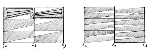
Figure 1. A classical illustration of the existence problem with Monge’s formulation: there is no optimal transport map from a segment $L_{1}$ to two parallel segments $L_{2}$ and $L_{3}$ (it is always possible to find a better one by replacing $h$ with $h/2$)

The non-symmetry comes from the constraint that $T$ should be a map. It makes it possible to merge mass but not to split mass. This difficulty is illustrated in Figure 1. Suppose you want to find the optimal transport from one vertical segment $L_{1}$ to two parallel segments $L_{2}$ and $L_{3}$. It is possible to split $L_{1}$ into segments of length $h$ mapped to $L_{2}$ and $L_{3}$ in alternance (Figure 1 left). For any length $h$, it is always possible to find a better map, i.e. with a lower value of the functional in $(C2)$, by splitting $L_{1}$ into smaller segments (Figure 1 right), therefore problem (M) does not have a solution within the set of admissible maps. This problem occurs whenever the source measure $\mu$ has mass concentrated on sets with zero geometric measure (like $L_{1}$).

1.2. The relaxation of Kantorovich for Monge’s problem

To overcome this difficulty, Kantorovich proposed a relaxation of problem (M) where mass can be both splitted and merged. The idea consists of manipulating measures on $\Omega\times\Omega$ as follows :

$$(K)\quad\quad\begin{array}[]{l}\mbox{min}\left\{\int\limits_{\Omega\times\Omega}c(x,y)d\gamma\ |\ \gamma\in\Pi(\mu,\nu)\right\}\\[14.22636pt] \mbox{where }\Pi(\mu,\nu)=\{\gamma\in{\mathcal{P}}(\Omega\times\Omega)\ |\ (P_{1})\sharp\gamma=\mu\ ;\ (P_{2})\sharp\gamma=\nu\}\end{array}$$

where $(P_{1})$ and $(P_{2})$ denote the two projections $(x,y)\in\Omega\times\Omega\mapsto x$ and $(x,y)\in\Omega\times\Omega\mapsto y$ respectively.

The pushforwards of the two projections $(P_{1})\sharp\gamma$ and $(P_{2})\sharp\gamma$ are called the marginals of $\gamma$. The probability measures $\gamma$ in $\Pi(\mu,\nu)$, i.e. that have $\mu$ and $\nu$ as marginals, are called transport plans. Among the transport plans, those that are in the form $(Id\times T)\sharp\mu$ correspond to a transport map $T$ :

Observation 1.

If $(Id\times T)\sharp\mu\in\pi(\mu,\nu)$, then $T$ pushes $\mu$ to $\nu$.

Proof.

$(Id\times T)\sharp\mu$ belongs to $\pi(\mu,\nu)$, therefore $(P_{2})\sharp(Id\times T)\sharp\mu=\nu$,
or $\left((P_{2})\circ(Id\times T)\right)\sharp\mu=\nu$, thus $T\sharp\mu=\nu$ ∎

With this observation, for transport plans of the form $\gamma=(Id\times T)\sharp\mu$, (K) becomes

$$\mbox{min}\left\{\int\limits_{\Omega\times\Omega}c(x,y)d\left((Id\times T)\sharp\mu\right)\right\}\quad=\quad\mbox{min}\left\{\int\limits_{\Omega}c(x,T(x))d\mu\right)$$

To help intuition, four examples of transport plans in 1D are depicted in Figure 2. The measure $\gamma$ on $\Omega\times\Omega$ is non-zero on subsets that contain points $(x,y)$ such that mass is transported from $x$ to $y$. The transport plans in the first two examples are in the form $(Id\times T)\sharp\mu$, i.e. they are derived from a transport map. The third and fourth ones do not admit a transport map, because they split a Dirac mass. The optimal transport plan for the case shown in Figure 1 is of the same nature. It is not in the form $(Id\times T)\sharp\mu$ because it splits the mass concentrated in $L_{1}$ into $L_{2}$ and $L_{3}$.

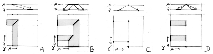
Figure 2. Four examples of transport plans in 1D. A: a segment is translated. B: a segment is splitted into two segments. C: a Dirac mass is splitted into two Dirac masses. D: a Dirac mass is splitted into two segments. The first two ones (A and B) are in the form $(Id\times T)\sharp\mu$ where $T$ is a transport map, whereas the third and fourth ones (C and D) are not, because they both split a Dirac mass.

At this point, a standard approach to tackle the existence problem is to find some regularity in both the functional and space of admissible transport plans, i.e. proving that the functional is smooth enough and finding a compact set of admissible transport plans. Since the set of admissible transport plans contains at least the product measure $\mu\otimes\nu$, it is non-empty, and existence can be proved using a topological argument that exploits the smoothness of the functional and the compactness of the set. Once the existence of a transport plan is proved, an interesting question is whether there exists a transport map that corresponds to this transport plan. Unfortunately, problem (K) does not directly exhibit the properties required by this path of reasoning. However, one can observe that (K) is a linearly constrained optimization problem. This calls for studying the dual formulation, as done by Kantorovich. This dual formulation has a nice structure, that allows answering the questions above (existence of a transport plan, and whether there is a transport map that corresponds to this transport plan when it exists).

1.3. The dual formulation of Kantorovich

The dual formulation can be stated as follows :

$$(D):\quad\quad\mbox{max}\left\{\int\limits_{\Omega}\phi d\mu+\int\limits_{\Omega}\psi d\nu\ |\ \begin{array}[]{ll}(C1)&\phi\in L^{1}(\mu);\psi\in L^{1}(\nu);\\ (C2)&\phi(x)+\psi(y)\leq c(x,y)\forall(x,y)\in\Omega\times\Omega\end{array}\right\}$$

Following the classical image that gives some intuition about this formula, imagine now that you are hiring a transport company to do the job for you. The company has a special way of calculating the price: the function $\phi(x)$ corresponds to what they charge you for loading at $x$, and $\psi(y)$ what they charge for unloading at $y$. The company tries to maximize profit (therefore is looking for a max instead of a min), but they cannot charge you more than what it will cost you if you do the job yourself $(C2)$.

The existence for $(D)$ is difficult to study, since the class of admissible functions that satisfy $(C1)$ and $(C2)$ is non-compact. However, more structure in the problem can be revealed by referring to the notion of c-transform, that exhibits a class of admissible functions with regularity :

Definition 1.

Given a function ${\mathcal{X}}:\Omega\rightarrow\bar{\mathbb{R}}$, the c-transform ${\mathcal{X}}^{c}$ is defined by :

$${\mathcal{X}}^{c}:=\inf\limits_{x\in\Omega}c(x,y)-{\mathcal{X}}(x)$$

• If for a function $\phi$ there exists a function ${\mathcal{X}}$ such that $\phi={\mathcal{X}}^{c}$, then $\phi$ is said to be c-concave;

• ${\bf\Psi}_{c}(\Omega)$ denotes the set of c-concave functions on $\Omega$.

It is now possible to make two observations, that allow us to restrict ourselves to the class of c-concave functions for the possible choices for $\phi$ and $\psi$ :

Observation 2.

If $(\phi,\psi)$ is admissible for $(D)$, then $(\phi,\phi^{c})$ is also admissible.

Proof.

$$\begin{array}[]{l}\left\{\begin{array}[]{l}\forall(x,y)\in\Omega\times\Omega,\phi(x)+\psi(y)\leq c(x,y)\\ \phi^{c}(y)=\inf\limits_{x\in\Omega}c(x,y)-\phi(x)\end{array}\right.\\ \begin{array}[]{lcl}\phi(x)+\phi^{c}(y)&=&\phi(x)+\inf_{x^{\prime}\in\Omega}\left(c(x^{\prime},y)-\phi(x^{\prime})\right)\\ &\leq&\phi(x)+c(x,y)-\phi(x)\\ &\leq&c(x,y)\end{array}\end{array}$$

∎

Observation 3.

If $(\phi,\psi)$ is admissible for $(D)$, then a better candidate can be found by replacing $\psi$ with $\phi^{c}$ :

Proof.

$$\left\{\begin{array}[]{lcl}\phi^{c}(y)&=&\inf\limits_{y\in\Omega}c(x,y)-\phi(x)\\ \forall x\in\Omega,\psi(y)&\leq&c(x,y)-\phi(x)\end{array}\right.\quad\quad\Rightarrow\quad\psi(y)\leq\phi^{c}(y)$$

∎

Therefore, we have $\min(K)\quad=\max\limits_{\psi\in{\bf\Psi}_{c}(\Omega)}\quad\int\limits_{\Omega}\psi d\mu+\int\limits_{\Omega}\psi^{c}d\nu$
I will not detail here the proof for the existence, the reader is referred to [29], Chapter 4. The idea is that we are now in a much better situation, since the class of admissible functions ${\bf\Psi}_{c}(\Omega)$ is compact (provided that we fix the value of $\Psi$ at one point of $\Omega$ to remove the translational invariance degree of freedom of the problem).

Since we have computer implementation in mind, our goal is to find a numerical algorithm to compute an optimal transport map $T$. At first sight, though the values of the functionals match at a solution of $(K)$ and $(D)$, it seems to be difficult to deduce $T$ from a solution to the dual problem $(D)$. However, there is a nice relation between the dual problem $(D)$ and the initial Monge’s problem $(M)$, detailed in [29], chapters 9 and 10. The main result characterizes the pairs of points $(x,y)$ that are connected by the transport plan :

Theorem 1.

$$\forall(x,y)\in\partial_{c}\psi,\nabla\psi(x)-\nabla_{x}c(x,y)=0$$

where $\partial_{c}\psi=\{(x,y)|\phi(x)+\psi(y)=c(x,y)\}$ denotes the so-called c-subdifferential of $\psi$.

Proof.

See [29] chapter 10.
I summarize the heuristic argument given at the beginning of the same chapter, that gives some intuition :
Consider a point $(x,y)$ on the c-subdifferential $\partial_{c}\psi$, that satisfies $\phi(y)+\psi(x)=c(x,y)\ (1)$.
By definition, $\phi(y)=\psi^{c}(y)=\inf\limits_{x}c(x,y)-\psi(x)$, thus $\forall\tilde{x},\phi(y)\leq c(\tilde{x},y)-\psi(\tilde{x})$, or $\phi(y)+\psi(\tilde{x})\leq c(\tilde{x},y)\ (2)$.
By substituting (1) into (2), one gets $\psi(\tilde{x})-\psi(x)\leq c(\tilde{x},y)-c(x,y)$ for all $\tilde{x}$.
Imagine now that $\tilde{x}$ follows a trajectory parameterized by $\epsilon$ and starting at $x$. One can compute the gradient along an arbitrary direction $w$ by taking the limit when $\epsilon$ tends to zero in the relation $\frac{\psi(\tilde{x})-\psi(x)}{\epsilon}\leq\frac{c(\tilde{x},y)-c(x,y)}{\epsilon}$. Thus we have $\nabla\psi(x)\cdot w\leq\nabla_{x}c(x,y)\cdot w$. The same derivation can be done with $-w$ instead of $w$, and one gets: $\forall w,\nabla\psi(x)\cdot w=\nabla_{x}c(x,y)\cdot w$, thus $\forall(x,y)\in\partial_{c}\psi,\nabla\psi(x)-\nabla_{x}c(x,y)=0$.
Note: the derivations above are only formal ones and do not make a proof. The proof requires a much more careful analysis, using generalized definitions of differentiability and tools from convex analysis. ∎

In the $L_{2}$ case, i.e. $c(x,y)=1/2\|x-y\|^{2}$, we have $\forall(x,y)\in\partial_{c}\psi,\nabla\psi(x)+y-x=0$, thus, whenever the optimal transport map $T$ exists, we have $T(x)=x-\nabla\psi(x)=\nabla(\|x\|^{2}/2-\psi(x))$. Not only this gives an expression of $T$, but also it allows characterizing $T$ as the gradient of a convex function, which is an interesting property since it implies that two “transported particles” $x_{1}\mapsto T(x_{1})$ and $x_{2}\mapsto T(x_{2})$ cannot collide, as shown below :

Observation 4.

If $c(x,y)$ = $1/2\|x-y\|^{2}$ and $\psi\in{\bf\Psi}_{c}(\Omega)$, then $\bar{\psi}:x\mapsto\bar{\psi}(x)=\|x\|^{2}/2-\psi(x)$ is convex (it is an equivalence if $\Omega=\mathbb{R}^{d}$).

Proof.

$$\begin{array}[]{lcl}\psi(x)&=&\inf\limits_{y}\frac{|x-y|^{2}}{2}-\phi(y)\\ &=&\inf\limits_{y}\frac{\|x\|^{2}}{2}-x\cdot y+\frac{\|y\|^{2}}{2}-\phi(y)\\ -\bar{\psi}(x)&=&\phi(x)-\frac{\|x\|^{2}}{2}=\inf\limits_{y}-x\cdot y+\left(\frac{\|y\|^{2}}{2}-\phi(y)\right)\\ \bar{\psi}(x)&=&\sup\limits_{y}x\cdot y-\left(\frac{\|y\|^{2}}{2}-\phi(y)\right)\end{array}$$

The function $x\mapsto x\cdot y-\left(\frac{\|y\|^{2}}{2}-\phi(y)\right)$ is linear in $x$, therefore the graph of $\bar{\psi}$ is the upper envelope of a family of hyperplanes, thus $\bar{\psi}$ is convex. ∎

Observation 5.

Consider the trajectories of two particles parameterized by $t\in[0,1]$, $t\mapsto(1-t)x_{1}+tT(x_{1})$ and $t\mapsto(1-t)x_{2}+tT(x_{2})$. If $x_{1}\neq x_{2}$ and for $0<t<1$ the particles cannot collide.

Proof.

By contradiction, suppose that you have $t\in(0,1)$ and $x_{1}\neq x_{2}$ such that:

$$\begin{array}[]{lcl}(1-t)x_{1}+tT(x_{1})&=&(1-t)x_{2}+tT(x_{2})\\ (1-t)x_{1}+t\nabla\bar{\psi}(x_{1})&=&(1-t)x_{2}+t\nabla\bar{\psi}(x_{2})\\ (1-t)(x_{1}-x_{2})+t(\nabla\bar{\psi}(x_{1})-\nabla\bar{\psi}(x_{2}))&=&0\\ \forall v,(1-t)v\cdot(x_{1}-x_{2})+tv\cdot(\nabla\bar{\psi}(x_{1})-\nabla\bar{\psi}(x_{2}))&=&0\\ \mbox{ take }v=(x_{1}-x_{2})\\ (1-t)\|x_{1}-x_{2}\|^{2}+t(x_{1}-x_{2})\cdot(\nabla\bar{\psi}(x_{1})-\nabla\bar{\psi}(x_{2}))&=&0\end{array}$$

which is a contradiction since this quantity is the sum of two strictly positive numbers ( recalling the definition of the convexity of $\bar{\psi}$: $\forall x_{1}\neq x_{2},(x_{1}-x_{2})\cdot(\nabla\bar{\psi}(x_{1})-\nabla\bar{\psi}(x_{2}))>0$ ).

∎

At this point, we know that when the optimal transport map exists, it can be deduced from the function $\psi$ using the relation $T(x)=\nabla\bar{\psi}=x-\nabla\psi$. We now consider some ways of finding the function $\psi$.

The classical change of variable formula gives:

$$\forall B,\int_{B}\mu(x)d\mu=\mu(B)=\nu(T(B))=\int_{B}\frac{1}{\det JT(x)}T(x)d\nu$$

where $JT$ denotes the Jacobian matrix of $T$.

If $\mu$ and $\nu$ both have a density $u$ and $v$ (i.e. $\forall B,\mu(B)=\int_{B}u(x)dx$ and $\nu(B)=\int_{B}v(x)dx$), then one can (formally) consider (1.3) in a pointwise manner :

$$\forall x\in\Omega,u(x)=\frac{1}{\det JT(x)}v(T(x))\ ;$$

injecting $T=\nabla\bar{\psi}$ and $JT=H\bar{\psi}$ in (1.3) gives:

(1) $$\forall x\in\Omega,u(x)=\frac{1}{\det H\bar{\psi}(x)}v(\nabla\bar{\psi}(x))$$

where $H\bar{\psi}$ denotes the Hessian of $\bar{\psi}$. Equation 1 is known as the Monge-Ampère equation. It is a highly non-linear equation, and its solution when it exists often has singularities. It is similar to the eikonal equation that characterizes the distance function and that has a singularity on the medial axis. Note that the derivations above are only formal, studying the solutions of the Monge-Ampère equation requires using more elaborate tools, and several types of weak solutions can be defined (viscosity solutions, solutions in the sense of Brenier, …).

Still keeping computer implementation in mind, one may consider three different problem settings :

• continuous: if $\mu$ and $\nu$ have a density $u$ and $v$, it is possible to numerically solve the Monge-Ampère equation, as done in [5] and [26];

• discrete: if both $\mu$ and $\nu$ are discrete (sums of Dirac masses), then finding the optimal transport plan becomes an assignment problem, that can be solved with some variants of linear programming techniques (see the survey in [7]);

• semi-discrete: if $\mu$ has a density and $\nu$ is discrete (sum of Dirac masses), then an optimal transport map exists. It has interesting connections with notions of computational geometry. The remainder of this paper considers this problem setting.

1.4. The semi-discrete case

I now consider that $\mu$ has a density $u$, and that $\nu=\sum_{i=1}^{k}\nu_{i}\delta_{p_{i}}$ is a sum of $k$ Dirac masses, that satisfies $\nu(\Omega)=\sum_{i=1}^{k}\nu_{i}=\mu(\Omega)$. Whenever $T$ exists, the pre-images of the Dirac masses $T^{-1}(p_{i})$ partition $\Omega$ almost everywhere. This subsection reviews the main results in [4], showing that this partition corresponds to a geometrical structure called a power diagram. Interestingly, from the point of view of computer implementation, the proof directly leads to a numerical algorithm, as experimented in 2D in [21] and in 3D further in this paper.

Definition 2.

Given a set $P$ of $k$ points $p_{i}$ in $\mathbb{R}^{d}$ and a set $W$ of $k$ real numbers $w_{i}$, the Voronoi diagram $\mbox{Vor}(P)$ and the power diagram $\mbox{Pow}_{W}(P)$ are defined as follows :

• The Voronoi diagram $\mbox{Vor}(P)$ is the partition of $\mathbb{R}^{d}$ into the subsets $\mbox{Vor}(p_{i})$ defined by :
  $\mbox{Vor}(p_{i}):=\{x|\|x-p_{i}\|^{2}<\|x-p_{j}\|^{2}\quad\forall j\neq i\}$;

• the power diagram $\mbox{Pow}_{W}(P)$ is the partition of $\mathbb{R}^{d}$ into the subsets $\mbox{Pow}_{W}(p_{i})$ defined by :
  $\mbox{Pow}_{W}(p_{i}):=\{x|\|x-p_{i}\|^{2}-w_{i}<\|x-p_{j}\|^{2}-w_{j}\quad\forall j\neq i\}$;

• the map $T_{W}$ defined by $\forall i,\forall p\in\mbox{Pow}_{W}(p_{i}),T_{W}(p)=p_{i}$ is called the assignment defined by the power diagram $\mbox{Pow}_{W}(P)$.

It can be shown that the assignment defined by a power diagram is an optimal transport map (the main argument of the proof is sketched further). Then one needs to determine - when it is possible - the parameters of this power diagram (i.e. the weights) that realize the optimal transport towards a given discrete target measure $\nu$. Intuitively, a power diagram may be thought-of as a generalization of the Voronoi diagram, with additional “tuning buttons” represented by the weights $w_{i}$. Changing the weight $w_{i}$ associated with a point $p_{i}$ influences the area and the measure $\mu(\mbox{Pow}_{W}(p_{i}))$ of its power cell (the higher the weight, the larger the power cell). Though the relation between the weights and the measures of the power cells is non-trivial, it is well behaved, and as shown below, one can prove the existence and uniqueness of a set of weights such that the measure of each power cell $\mu(\mbox{Pow}_{W}(p_{i}))$ matches a prescribed value $\nu_{i}$. In this case, the prescribed measures $\nu_{i}$ are referred to as capacity constraints, and the power diagram is said to be adapted to the capacity constraints. At this point, since we already know that the assignment defined by a power diagram is an optimal transport map, then we are done (i.e. the assignment defined by the power diagram is the optimal transport map that we are looking for). I shall now give more details about the proofs of the two parts of the reasoning.

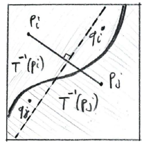
Figure 3. Illustration of the (by contradiction) argument that the common boundary between the pre-images of $p_{i}$ and $p_{j}$ is contained by a straight line orthogonal to $[p_{i},p_{j}]$.

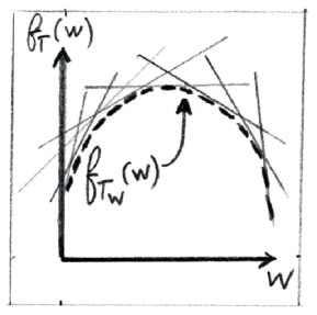
Figure 4. The weight vector that defines an optimal transport map can be found as the maximizer of a convex function, defined as the lower envelope of a family of linear functions.

Theorem 2.

Given a set of points $P$ and a set of weights $W$, the assignment $T_{P,W}$ defined by the power diagram is an optimal transport map.

Proof.

I give here the main idea of the proof (see [4] for the complete one). The main argument is that if $T$ is an optimal transport map, then the common boundary of the pre-images $T^{-1}(p_{i})$ and $T^{-1}(p_{j})$ of two Dirac masses is a straight line orthogonal to the segment $[p_{i},p_{j}]$. The argument, obtained by contradiction, is illustrated in Figure 4. Suppose that the common boundary between the pre-images $T^{-1}(p_{i})$ and $T^{-1}(p_{j})$ is not a straight line (thick curve in the figure), then one can find a straight line orthogonal to the segment $[p_{i},p_{j}]$ that has an intersection with the common boundary (dashed line in the figure), and two points $q_{i}$ and $q_{j}$ located as shown in the figure. Then, it is clear (by the Pythagorean theorem) that re-assigning $q_{j}$ to $T^{-1}(p_{i})$ and $q_{i}$ to $T^{-1}(p_{j})$ lowers the transport cost, which contradicts the initial assumption. It is then possible to establish that the pre-images correspond to power cells, by invoking some properties of power diagrams [3]. ∎

Theorem 3.

Given a measure $\mu$ with density, a set of points $(p_{i})$ and prescribed masses $\nu_{i}$ such that $\sum\nu_{i}=\mu(\Omega)$, there exists a weights vector $W$ such that $\mu(\mbox{Pow}_{W}(p_{i}))=\nu_{i}$.

Proof.

Consider the function $f_{T}(W)=\int_{\Omega}\|x-T(x)\|^{2}-w_{T(x)}d\mu$, where $T:\Omega\rightarrow P$ is an arbitrary assignment. One can observe that:

• If the assignment $T$ is fixed, $f_{T}(W)=\int_{\Omega}\|x-T(x)\|^{2}d\mu-\sum_{i=1}^{k}w_{i}\mu(T^{-1}(p_{i}))$ is affine in $W$. In Figure 4, the graph of $f_{T}(W)$ for a fixed assignment $T$ corresponds to one of the straight lines (note that in the figure, the “W axis” symbolizes $k$ coordinates);

• we now consider a fixed value of $W$ and different assignments $T$. Among all the possible $T$’s, it is clear that $f_{T}(W)$ is minimized by $T_{W}$, the assignment defined by the power diagram with weights $W$ (the definition of the power cell minimizes at each point of $\Omega$ the integrand in the equation of $f_{T}(W)$).

Now take $T=T_{W}$ in $f_{T}(W)$, in other words, consider the function $f_{T_{W}}(W)$. Its graph, depicted as a dashed curve in Figure 4, is the lower envelope of a family of hyperplanes, thus it is a concave function, with a single maximum. For the next steps of the proof, we now need to compute the gradient $\nabla_{W}f_{T_{W}}(W)$. Note that when computing the variations of $f_{T_{W}}(W)$, both the argument $W$ of $f$ and the parameter $T_{W}$ change, making the computations quite involved. When $T_{W}$ changes, the power cells change, and one needs to compute integrals over varying domains. However, it is possible to drastically simplify computations by using the envelope theorem. Given a parameterized family of functions $f_{T}(W)$ (in our case, the parameter is $T$), whenever the gradient of $\nabla_{W}f_{T_{W}}(W)$ exists, it is equal to the gradient $\nabla_{W}f_{T^{*}}(W)$ computed at the minimizer $T^{*}$ ($f_{T_{W}}$ in our case). In other words, when computing the gradients, one can directly use the expression of $f_{T}(W)$ and ignore the variations of $T$ in function of $W$. In Figure 4, it means that the tangent to $f_{T_{W}}$ at $W$ corresponds to the (linear) graph of $f_{T}(W)$ with a fixed $T=T_{W}$. Note that in our case, the so-called choice set, i.e. where $T$ is chosen, is the set of all the assignments between $\Omega$ and $P$. This requires a special version of the envelope theorem that works for such a general choice sets [23].

One can see that the components of the gradient correspond to the (negated) measures of the power cells :

$$\begin{array}[]{lcl}\frac{\partial f_{T_{W}}(W)}{\partial w_{i}}&=&\nabla_{W}\left(\underbrace{\int_{\Omega}\|x-T(x)\|^{2}d\mu}_{\mbox{constant}(W)}-\sum\limits_{i=1}^{k}w_{i}\mu(T^{-1}_{W}(p_{i}))\right)\\[34.1433pt] &=&-\mu(T_{W}^{-1}(p_{i}))=-\mu(\mbox{Pow}_{W}(p_{i}))\end{array}$$

We are now in a very good situation to establish the existence and uniqueness of the weight vector $W$ that realizes the optimal transport map. The idea is to use $f_{T_{W}}$ to construct a function $g$ that has a global maximum realized at a weight vector such that the measures of the power cells match the prescribed measures. Consider the function $g$ defined by $g(W)=f_{T_{W}}(W)+\sum_{i}\nu_{i}w_{i}$. The components of the gradient of $g$ are given by $\partial g/\partial w_{i}=-\mu(\mbox{Pow}_{W}(p_{i}))+\nu_{i}$. This function is also concave (it is the sum of a concave function plus a linear one), therefore it has a unique global maximum where the gradient is zero. Therefore, at the maximum of $g$, for each power cell, the measure $\mu(\mbox{Pow}_{W}(p_{i}))$ matches the prescribed measure $\nu_{i}$. ∎

Besides showing the existence of a semi-discrete transport map and characterizing it as the assignment defined by a power diagram, the proof in Theorem 3 directly leads to a numerical algorithm, as shown in [21], described in Section 2 further. A similar algorithm can be obtained by starting from a discrete version of the Monge-Ampere equation and the characterization of $T$ as the gradient of a piecewise linear convex function[13].

1.5. Relation with Kantorovich’s dual formulation

It is interesting to see the relation between the proof of Aurenhammer et.al that does not use the formalism of optimal transport, and the dual formulation of optimal transport. Interestingly, one can remark that the same argument (lower envelope of hyperplanes) is used to establish the concavity of $f_{T_{W}}$ in Theorem 3 and the convexity of $\bar{\psi}$ in Observation 4. The relation between both formulations can be further explained if we link the Kantorovich potential $\phi$ and the weights $w_{i}$ with the relation $\phi(y_{i})=1/2w_{i}$. For instance, injecting $\phi(y_{i})=1/2w_{i}$ and $c(x,y)=1/2\|x-y\|^{2}$ into $\psi(x)=\phi^{c}(x)=\inf_{y}c(x,y)-\phi(y)$ gives $\psi(x)=1/2\inf_{i}\|x-y_{i}\|^{2}-w_{i}$. This corresponds to the definition of the power cells (intuitively, the $\inf$ in the definition of $\phi^{c}$ is the same as the $\inf$ in the definition of the power cell). Now consider $T(x)=x-\nabla\psi(x)$. Still using the expression of $\psi(x)$ above, we get $T(x)=x-1/2\nabla_{x}(\|x-y_{i}\|^{2}-w_{i})=y_{i}$. This connects the characterization of $T$ as the solution of $\nabla\phi(x)-\nabla_{x}c(x,y)=0$ (Theorem 1) with the characterization of $T$ as the assignment defined by the power diagram (Theorem 3). This corresponds to the point of view developed in [13].

Figure 5. Left: random points (black dots), Voronoi diagram and cell centroids (gray dots); Right: a barycentric Voronoi diagram is a local minimizer of $Q$.

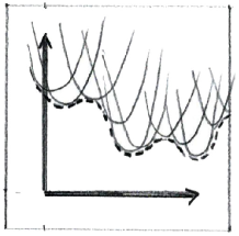
Figure 6. The quantization noise power $Q$ minimized in vector quantization is a lower envelope.

1.6. Relation with optimal sampling

In this section, I exhibit some relations between semi-discrete optimal transport and another problem referred to as optimal sampling (or vector quantization). Given a compact $\Omega\subset\mathbb{R}^{d}$, a measure $\mu$, and a set of $k$ points $Y$ in $\mathbb{R}^{d}$, the quantization noise power of $Y$ is defined as :

(2) $$Q(Y):=\int_{\Omega}\min_{i}\|x-y_{i}\|^{2}d\mu=\sum\limits_{i=1}^{k}\int_{\mbox{Vor}(y_{i})}\|x-y_{i}\|^{2}d\mu$$

The quantization noise power measures how good $Y$ is at “sampling” $\Omega$ (the smaller, the better), see the survey in [10]. The vector quantization problem consists in minimizing $Q(Y)$ (i.e. finding the poinset $Y$ that best samples $\Omega$). This notion comes from signal processing theory, and was used to find the optimal assignment of frequency bands for multiplexing communications in a single channel [19]. Designing a numerical algorithm that optimizes $Q$ requires to evaluate the gradient of $Q$. This requires computing integrals over varying domains (since the Voronoi cells of the $y_{i}$’s depend on the $y_{i}$’s), which requires several pages of careful derivations, as done in [14, 10]. At the end, most of the terms cancel-out, leaving a simple formula (see below). One can note the similarity between the quantization noise power (Equation 2) and the objective function maximized by the weight vector in semi-discrete optimal transport (proof of Theorem 3). This suggests using the same type of argument (envelope theorem) to directly obtain the gradient of $Q$ :

Observation 6.

The function $Q$ is of class $C^{1}$ (at least ) and the components of its gradient relative to one of the point $y_{i}$ is given by:

$$\nabla_{y_{i}}Q(Y)=2m_{i}(y_{i}-g_{i})$$

where $m_{i}=\mu(\mbox{Vor}(y_{i}))=\int_{\mbox{Vor}(y_{i})}d\mu$ denotes the mass of the Voronoi cell $\mbox{Vor}(y_{i})$ and $g_{i}=1/m_{i}\int_{\mbox{Vor}(y_{i})}xd\mu$ denotes the centroid of the Voronoi cell $\mbox{Vor}(y_{i})$.

Proof.

Consider the function $Q_{T}(Y):=\int_{\Omega}\|x-T(x)\|^{2}d\mu$, parameterized by an assignment $T:\Omega\rightarrow Y$. We are in a setting similar to semi-discrete optimal transport (Section 1.4), except that the function $Q_{T}(Y)$ is quadratic (see Figure 6), whereas $F_{T}(W)$ is linear (Figure 4). We have :

• $Q(Y)=Q_{T_{\mbox{Vor}}}(Y)$;

• for a given $Y$, $T_{\mbox{Vor}}$ is the unique affectation that minimizes $Q_{T}(Y)$.

By the envelope theorem, we have:

$$\begin{array}[]{lcl}\nabla Q(Y)&=&\nabla Q_{T_{\mbox{Vor}}}(Y))=\nabla\sum_{i}\int\limits_{\mbox{Vor}(y_{i})}(x^{2}-2x\cdot y_{i}+y_{i}^{2})d\mu\\[11.38109pt] &=&\sum_{i}\left(\nabla\int\limits_{\mbox{Vor}(y_{i})}x^{2}d\mu-2\nabla\int\limits_{\mbox{Vor}(y_{i})}x\cdot y_{i}d\mu+\nabla\int\limits_{\mbox{Vor}(y_{i})}y_{i}^{2}d\mu\right)\\[17.07164pt] \nabla_{y_{i}}Q(y)&=&-2y_{i}\int\limits_{\mbox{Vor}(y_{i})}xd\mu+2y_{i}\int\limits_{\mbox{Vor}(y_{i})}d\mu\\[11.38109pt] &=&-2m_{i}g_{i}+2m_{i}y_{i}=2m_{i}(y_{i}-g_{i})\end{array}$$

∎

This directly gives the expression of the gradient of $Q$ and explains why most of the terms cancel out in the derivations conducted in [14]. I mention that the same result can be obtained in a more general setting with Reynold’s transport theorem [25] (that deals with functions integrated over varying domains).

However, the envelope argument cannot be used to compute the Hessian of $Q$ (second order derivatives), and the structure of the formulas [14, 11, 18] do not suggest that direct computation can be avoided for them. Note also that $Q$ is the lower envelope of a family of parabola (instead of a family of hyperplanes), therefore the concavity argument does not hold, and the graph of $Q$ has many local minima (as depicted in Figure 6). The local minima of $Q$, i.e. the point sets $Y$ such that $\nabla Q=0$, satisfy $\forall i,y_{i}=g_{i}$, in other words, the position at each point $y_{i}$ corresponds to the centroids of the Voronoi cell associated with $y_{i}$. For this reason, a stationary point of $Q$ is called a centroidal Voronoi tessellations. To compute a centroidal Voronoi tessellation, it is possible to iteratively move each point towards the centroid of its Voronoi cell (Lloyd relaxation [19]), which is equivalent to minimizing $Q$ with a gradient descent method [10]. It is also possible to minimize $Q$ with Newton-type methods [18] that show faster convergence.

More relations between semi-discrete optimal transport and vector quantization can be exhibited by considering a power diagram as the intersection between a $d+1$ Voronoi diagram and $\mathbb{R}^{d}$ :

Observation 7.

The $d$-dimensional power diagram $\mbox{Pow}_{W}(Y)$ corresponds to the intersection between the $d+1$ dimensional Voronoi diagram $\mbox{Vor}(\hat{Y})$ and $\mathbb{R}^{d}$, where the $\mathbb{R}^{d+1}$ lifting $\hat{y_{i}}$ of $y_{i}$ is defined by :

$$\hat{y_{i}}=\left(\begin{array}[]{c}y_{i,1}\\ y_{i,2}\\ \vdots\\ y_{i,d}\\[5.69054pt] h_{i}=\sqrt{w_{M}-w_{i}}\end{array}\right)$$

where $y_{i,j}$ denotes the $j$-th coordinate of point $y_{i}$, and where $w_{M}$ denotes the maximum of all weights $\mbox{Max}(w_{i})$.

Proof.

$$\begin{array}[]{l}\mbox{Vor}(\hat{y}_{i})\cap\mathbb{R}^{d}=\{x\quad|\quad\|\hat{x}-\hat{y}_{i}\|^{2}<\|\hat{x}-\hat{y}_{j}\|^{2}\ \forall j\neq i\}\\[5.69054pt] \begin{array}[]{lcl}&=&{\small\left\{x\quad|\quad\left\|\left[\begin{array}[]{c}x\\[2.84526pt] 0\end{array}\right]-\left[\begin{array}[]{c}y_{i}\\[2.84526pt] \sqrt{w_{M}-w_{i}}\end{array}\right]\right\|^{2}<\par\left\|\left[\begin{array}[]{c}x\\[2.84526pt] 0\end{array}\right]-\left[\begin{array}[]{c}y_{j}\\[2.84526pt] \sqrt{w_{M}-w_{j}}\end{array}\right]\right\|^{2}\ \forall j\neq i\right\}}\\[17.07164pt] &=&\{x\quad|\quad\|x-y_{i}\|^{2}-w_{i}+w_{M}<\|x-y_{j}\|^{2}-w_{j}+w_{M}\ \forall j\neq i\}\\[5.69054pt] &=&\{x\quad|\quad\|x-y_{i}\|^{2}-w_{i}<\|x-y_{j}\|^{2}-w_{j}\ \forall j\neq i\}\\[5.69054pt] &=&\mbox{Pow}_{W}(y_{i})\end{array}\end{array}$$

∎

We can now see a relation between vector quantization and semi-discrete optimal transport :

Observation 8.

The quantization noise power $\hat{Q}(\hat{Y})$ computed in $\mathbb{R}^{d+1}$ corresponds to the term $f_{T_{W}}(W)$ of the function maximized by the weight vector that defines a semi-discrete optimal transport map plus the constant $w_{M}\mu(\Omega)$.

Proof.

$$\begin{array}[]{lcl}\hat{Q}(\hat{Y})&=&\sum\limits_{i}\int\limits_{\mbox{Vor}(\hat{y}_{i})\cap{\mathbb{R}^{d}}}\|\hat{x}-\hat{y}_{i}\|^{2}d\mu\\[22.76219pt] &=&\sum\limits_{i}\int\limits_{\mbox{Pow}_{W}(y_{i})}\|x-y_{i}\|^{2}-w_{i}+w_{M}d\mu\\[11.38109pt] &=&f_{T_{W}}(W)+w_{M}\mu(\Omega)\end{array}$$

∎

The quantization noise power $Q$ is already known to be of class $C^{2}$ almost everywhere [18]. As a consequence of this observation, since the function $f_{T_{W}}(W)$ can be obtained through the change of variable $h_{i}=\sqrt{w_{M}-w_{i}}$, it is also of class $C^{2}$ almost everywhere. This gives more justification for using a quasi-Newton method to find the maximum of $g$ as done in [21] and in this paper (but note that a complete justification would require to find some bounds on the eigenvalue of the Hessian).

Another consequence of this observation is that given $\Omega\subset\mathbb{R}^{d}$, a measure $\mu$ and a pointset $Y$, optimizing $\hat{Q}$ for the first $d$ coordinates moves the points in a way that minimizes the quantization noise power, and optimizing for the $d+1$ coordinate computes the weights of a power diagram that defines an assignment that transports $\mu$ to the points. Interestingly, the first problem has multiple local minima, whereas the second one admits a global maximum.

2. Numerical Algorithm

I shall now explain how to use the results in Section 1.4 and turn them into an efficient numerical algorithm. The algorithm is a variation of the one in [21]. Besides generalizing it to the 3d case, I make some observations that improve the efficiency of the multilevel optimization method.

The input of the algorithm is a measure $\mu$, represented by a simplicial complex $M$ (i.e. an interconnected set of tetrahedra in 3D), a set $Y$ of $k$ points $y_{i}$ and $k$ masses $\nu_{i}$ such that $\sum\nu_{i}=\mu(M)$ where $\mu(.)$ is defined as follows : For a set $B\subset\mathbb{R}^{3}$, the measure $\mu(B)$ corresponds to the volume of the intersection between the tetrahedra of $M$ and $B$. Optionally, $M$ can have a density linearly interpolated from its vertices. In this setting, the measure of $B$ corresponds to the integral of the linearly interpolated density on the intersection between $B$ and the tetrahedra of $M$.

The weight vector that realizes the optimal transport can be obtained by maximizing the function $g(W)$ using different numerical methods. The single-level version of the algorithm in [21] is outlined in Algorithm 1 :

Data: A tetrahedral mesh $M$, a set of points $Y$ and masses $\nu_{i}$ such that $\mu(M)=\sum\nu_{i}$

Result: The weight vector $W$ that determines the optimal transport map $T$ from $M$ to $\sum\nu_{i}\delta_{y_{i}}$

$W\leftarrow 0$

(1) while  $\|\nabla g(W)\|^{2}<\epsilon\$ do

       (2) Compute $\mbox{Vor}_{W}(Y)\cap M$

      [2mm] (3) Compute $g(W)=\sum_{i}\int\limits_{\mbox{Pow}_{W}(y_{i})\cap M}\|x-y_{i}\|^{2}-w_{i}d\mu+\sum_{i}\nu_{i}w_{i}$

      [2mm] (4) Compute $\nabla g(W)=-\mu(\mbox{Pow}_{W}(y_{i}))+\nu_{i}$

       (5) update $W$ with L-BFGS

end while

Algorithm 1 Semi-discrete optimal transport (single-level algorithm)

To facilitate reproducing the results, I give more details about each step of the algorithm: (1): note that the components of the gradient of $g$ correspond to the difference between the prescribed measures $\nu$ and the measures of the power cells. This gives an interpretation of the norm of the gradient of $g$, and helps choosing a reasonable $\epsilon$ threshold. In the experiments below, I used $\epsilon=0.01*\mu(M)/\sqrt{k}$. (2): the algorithm that computes the intersection between a power diagram and a tetrahedral mesh is detailed further (Algorithm 2). (3),(4): once the intersection $\mbox{Vor}_{W}(Y)\cap M$ is computed, the terms $g(W)$ and $\nabla g(W)$ are obtained by summing the contributions of each intersection (grayed area in Figure 7). (5): To maximize $g$, as in [21], I use the L-BFGS numerical optimization method [16]. An implementation is available in [17].

2.1. Computing the intersection between a tetrahedral mesh and a power diagram

To adapt the 2d algorithm in [21] to the 3d case, the only required component is a method that computes the intersection between a tetrahedral mesh and a power diagram (step (2) in Algorithm 1) :

Data: A tetrahedral mesh $M$, a set of points $Y$ and a weight vector $W$

Result: The intersection $\mbox{Vor}_{W}(Y)\cap M$

S: Stack(couple(tet index, point index))

foreach  tetrahedron $t\in M$ do

       if  $t$ is not marked  then

             (1) $i\leftarrow i\ |\ \mbox{Pow}_{W}(y_{i})\cap t\neq\emptyset$

             Mark(t,i)

             Push(S, (t,i))

             while S is not empty do

                   (t,i) $\leftarrow$ Pop(S)

                   (2) P: Convex $\leftarrow\mbox{Pow}_{W}(y_{i})\cap t$

                   (3) Accumulate(P)

                   (4) foreach j neighbor of i in P do

                         if $(t,j)$ is not marked then

                               Mark($t,j$);  Push(S, ($t,j$))

                         end if

                        

                   end foreach

                  5 foreach $t^{\prime}$ neighbor of $t$ in P do

                         if $(t^{\prime},i)$ is not marked then

                               Mark($t^{\prime},i$);  Push(S, ($t^{\prime},i$))

                         end if

                        

                   end foreach

                  

             end while

            

       end if

      

end foreach

Algorithm 2 Computing $\mbox{Pow}_{W}(Y)\cap M$ by propagation

The algorithm works by propagating simultaneously over the tetrahedra and the power cells. It traverses all the couples $(t,i)$ such that the tetrahedron $t$ has a non-empty intersection with the power cell of $y_{i}$. (1): Propagation is initialized by starting from an arbitrary tetrahedron $t$ and a point $y_{i}$ that has a non-empty intersection between its power cell and $t$. I use the point $y_{i}$ that minimizes its power distance $\|y_{i}-.\|^{2}-w_{i}$ to one of the vertices of $t$. (2): a tetrahedron $t$ and a power cell $\mbox{Pow}_{W}{y_{i}}$ can be both described as the intersection of half-spaces, as well as the intersection $t\cap\mbox{Pow}_{W}{y_{i}}$, computed using re-entrant clipping (each half-space is removed iteratively). I use two version of the algorithm, a non-robust one that uses floating point arithmetics, and a robust one [15], that uses arithmetic filters [22], expansion arithmetics [28] and symbolic perturbation [12]. Both predicates and power diagram construction algorithm are available in PCK (Predicate Construction Kit) part of my publically available “geogram” programming library. (3) the contribution of each intersection $P=t\cap\mbox{Pow}_{W}{y_{i}}$ is added to $g$ and $\nabla g$.

The convex $P$ is illustrated in the (2d) figure 7 as the grayed area (in 3d, $P$ is a convex polyhedron). The algorithm then propagates to both neighboring tetrahedra and points. (4): each portion of a facet of $t$ that remains in $P$ triggers a propagation to a neighboring tetrahedron $t^{\prime}$. In the 2d example of Figure 7, this corresponds to edges $e_{1}$ and $e_{4}$ that trigger a propagation to triangles $t_{2}$ and $t_{1}$ respectively. (5): each facet of $P$ generated by a power cell facet triggers propagation to a neighboring point. In the 2d example of the figure, this corresponds to edges $e_{2}$ and $e_{3}$ that trigger propagation to points $y_{j_{1}}$ and $y_{j_{2}}$ respectively.

This algorithm is parallelized, by partitioning the mesh $M$ into $M_{1}$, $M_{2}$, …$M_{nb\_cores}$ and by computing in each thread $M_{thrd}\cap\mbox{Pow}_{W}(Y)$.

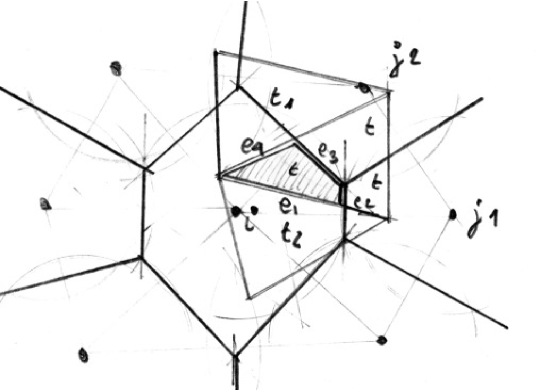
Figure 7. Computing the intersection between a power diagram and a tetrahedral mesh by propagation.

nb masses $k$	1000	2000	5000	10000	30000	50000	100000
nb iter	146	200	328	529	1240	1103	1102
time (s)	2.8	6.4	21	65	232	568	847

Table 1. Statistics for a simple translation scenario with the single-level algorithm. The threshold for $\|\nabla g\|^{2}$ is set to $\epsilon=0.01*\mu(M)/\sqrt{k}$.

I conducted a simple experiment, where $M$ is a tessellated sphere with 2026 tetrahedra, and $Y$ a sampling of the same sphere shifted by a translation vector of three times the radius of the sphere. The statistics in Table 1 obtained with a standard PC show that the single-level algorithm does not scale-up well with the number of points and starts taking a signiffficant time for processing 10K masses and above. This confirms the observation in [21]. This is because at the initial iteration, all the weights are zero, and the power diagram corresponds to the Voronoi diagram of the points $y_{i}$. At this step, only some points $y_{i}$ on the border of the pointset have a Voronoi cell that “see” the mesh $M$ (i.e. that have a non-empty intersection with it). It takes many iteration to compute the weights that “shift” the concerned power cells onto $M$ and allow inner points to see $M$. It is only once all the points of $Y$ “see” $M$ that the numerical method can capture the trend of $g$ around the maximum (and then it takes a small number of iterations to the algorithm to balance the weights). Intuitively, $Y$ is “peeled” only one layer of points at a time. The bad effect on performances is even more important than in [21], because in the 3d setting, the proportion of “inner” points relative to the number of points on the border of the pointset is larger than in 2d.

2.2. Multi-level algorithm

To improve performances, I follow the approach in [21], that uses a multilevel algorithm. The idea consists in “bootstrapping” the algorithm on a coarse sub-sampling of the pointset. The “peeling” effect mentioned in the previous paragraph is limited since we have a small number of points. Then the algorithm is run with a larger number of points, using the previously computed weights as an initialization. The set of points can be decomposed into multiple level of increasing resolution. The complete algorithm will be detailed below (Algorithm 3).

nb masses	1000	2000	5000	10000	30000	50000	100000
deg. 0 time (s)	2.5	6	19	38	184	356	959
deg. 1 time (s)	1	2	6	14	54	103	172
deg. 2 time (s)	1.4	2.2	6	16	58	138	172
BRIO/deg. 2 time (s)	1	1.65	3.4	9	26	62	106
single level time (s)	2.8	6.4	21	65	232	568	847

Table 2. Statistics for a simple translation scenario with the multi-level algorithm. The mesh $M$ has 61233 tetrahedra. Timings are in seconds. Each level is initialized from the previous one with regressions of different degrees.

To further improve the speed of convergence, I use the remark in Section 1.5 that the weights $w_{i}$ corresponds to the potential $\phi$ evaluated at $y_{i}$ (with a 1/2 factor). For a translation, we know that $T^{-1}(y)=y-V=y-\nabla\phi$, therefore $\phi(y)=V\cdot y$ where $V$ denotes the translation vector. In more general settings, $\phi$ is still likely to be quite regular (except on its singularities where $T$ is discontinuous). When initializing a level from the previous one, this suggests initializing the new $w_{i}$’s from a regression of their nearest neighbors computed at the previous level. Table 2 shows the statistics for initialization with the nearest neighbor (deg. 0), linear regression with 10 nearest neighbors (deg. 1) and quadratic regression with 20 nearest neighbors (deg. 2). As can be seen, initializing with linear regression results in a significant speedup. In this specific case though, quadratic regression does not gain anything. It is not a big surprise since we know already that $\phi(y)=V\cdot y$ is linear in this specific case, but it can slightly improve performances in more general settings, as shown further. Finally, it is possible to gain another x2 speedup factor : the algorithm that we use to compute the power diagrams [2] sorts the points with a multilevel spatial reordering method, that makes it very efficient. It is possible to use the same multilevel spatial ordering for both the numerical optimization and for computing the power diagrams (BRIO/deg. 2 row in the table). Since only the weights change during the iterations, this order needs to be computed once only, at the beginning of the algorithm. Note the overall 8x acceleration factor as compared to the single-level algorithm in Table 1 (repeated in the last row of Table 2 to ease comparison). The complete multi-level algorithm is summarized below :

Data: A tetrahedral mesh $M$, a set of points $Y$ and masses $\nu_{i}$ such that $\mu(M)=\sum\nu_{i}$

Result: The weight vector $W$ that determines the optimal transport map $T$ from $M$ to $\sum\nu_{i}\delta_{y_{i}}$

Apply a random permutation to the points $Y$

(1) Partition the interval of indices $[1,k]$ of $Y$ into $n_{l}$ intervals $[b_{l},e_{l}]$ of increasing size

foreach level $l$ do

       (2) Sort the points $y_{b_{l}}\ldots Y_{e_{l}}$ spatially

       (3) For each $i$, $\nu_{i}\leftarrow|M|/e_{l}$

       (4) Interpolate the weights $w_{b_{l}}\ldots w_{e_{l}}$ from the already computed weights $w_{1}\dots w_{b_{l}-1}$

       Optimize the weights using Algorithm 1

end foreach

Algorithm 3 Semi-discrete optimal transport (multi-level algorithm)

In my implementation, for step (1), the ratio between the number of points in a level and in the rest of the points is set to 0.125. For the spatial sort in step (2), the algorithm, available in “geogram”, was inspired by the variant of the Hilbert sort implemented in [9]. (3): Before computing the optimal transport maps, since the number of points changes at each level, the masses of the points need to be updated. At step (4), to determine the weight of a new point $w_{i}$, I use linear least squares with 10 nearest neighbors for degree 1 and quadratic least squares with 20 nearest neighbors for degree 2.

The influence of the degree of the regression is evaluated in Table 3 for a configuration where a sphere is splitted into two spheres (first row in Figure 8). Unlike in the previous translation case, in this configuration the potential $\phi$ is non-linear (see the deformations of the spheres), and a higher degree regression slightly improves the speed of convergence for a large number of points, since it captures more variations of $\phi$ and better initializes $W$.

nb masses	1000	2000	5000	10000	30000	50000	100000
BRIO/deg. 1 time (s)	1	1.7	3.5	9.8	25	61.7	122
BRIO/deg. 2 time (s)	0.9	1.6	3.5	8.4	28.3	61.4	112

Table 3. Statistics for splitting a sphere into two spheres with the multi-level algorithm. Timings are in seconds. Each level is initialized from the previous one with regressions of different degrees.

2.3. Using semi-discrete transport to approximate the transport between two tetrahedral meshes

I now consider the case where the input is a pair of tetrahedral meshes $M$ and $M^{\prime}$. The goal is now to generate a sequence of tetrahedral meshes that realize an approximation of the optimal transport between $M$ and $M^{\prime}$. The algorithm is outlined below :

Data: Two tetrahedral meshes $M$ and $M^{\prime}$, and $k$ the desired number of vertices in the result

Result: A tetrahedral mesh $G$ with $k$ vertices and a pair of points $p_{i}^{0}$ and $p_{i}^{1}$ attached to each vertex. Transport is parameterized by time $t\in[0,1]$ with $p_{i}(t)=(1-t)p_{i}^{0}+tp_{i}^{1}$.

(1) Sample $M^{\prime}$ with a set $Y$ of $k$ points

(2) Compute the weight vector $W$ that realizes the optimal transport between $M$ and $Y$ (Algorithm 3)

(3) Compute $E=\mbox{Del}(Y)|M^{\prime}$ and $F=\mbox{Pow}_{W}(Y)|M$  ;  Tets(G) $\leftarrow E\cap F$

(4) Foreach $i\in[1\ldots k]$, $(p_{i})^{0}\leftarrow\mbox{centroid}(\mbox{Pow}_{W}(y_{i})\cap M)\quad;\quad(p_{i})^{1}\leftarrow y_{i}$

Algorithm 4 Approximated optimal transport between two tetrahedral meshes

The different steps of this algorithm are implemented as follows: (1): to compute a homogeneous sampling, I initialize $Y$ with a centroidal Voronoi tessellation (see Section 1.6). (3): the main difficulty consists in finding the discontinuities in $T$ and avoid generating tetrahedra that cross them. To detect the discontinuities in $T$, I consider that the Voronoi diagram $\mbox{Vor}(Y)$ that samples $M^{\prime}$ evolves towards the power diagram $\mbox{Pow}_{W}(Y)$ that samples $M$ (note that this evolution goes backwards, from $M^{\prime}$ to $M$). Thus, the tetrahedra that are kept are those that are present both in the dual $\mbox{Del}(Y)$ of $\mbox{Vor}(Y)$ (Delaunay triangulation) and the dual $\mbox{Reg}_{W}(Y)$ of $\mbox{Pow}_{W}(Y)$ (regular weighted triangulation). (4) Finally, the geometry $p_{i}^{0}$ of each vertex of $G$ at initial time $t=0$ is determined as the centroid of the power cell $\mbox{Pow}_{W}(y_{i})\cap M$. The geometry $p_{i}^{1}$ at final time $t=1$ is simply $y_{i}$.

3. Results and conclusions

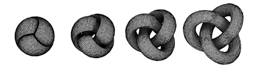
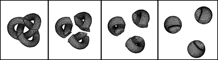
Figure 8. Some examples of semi-discrete optimal transport with topology changes.

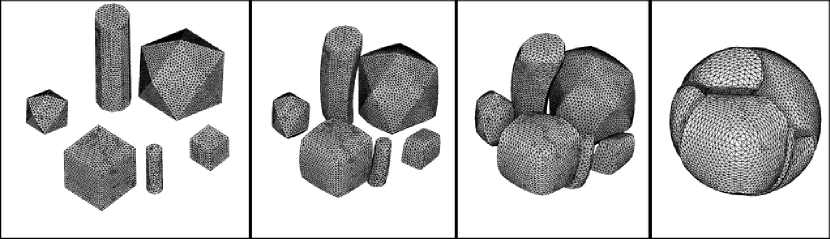
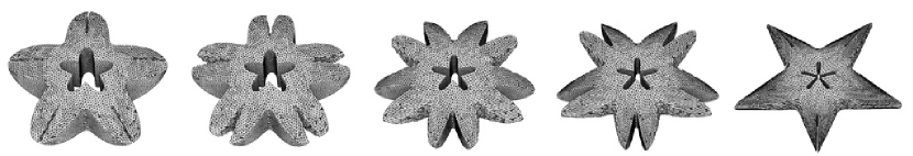
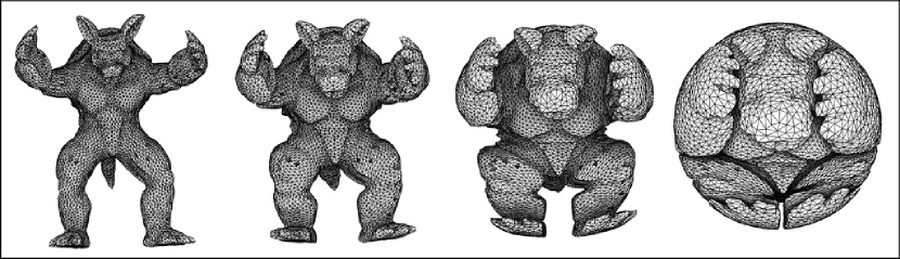
Figure 9. More examples of semi-discrete optimal transport. Note how the solids deform and merge to form the sphere on the first row, and how the branches of the star split and merge on the second row.

nb masses	1000	2000	5000	10000	30000	50000	$10^{5}$	$3\times 10^{5}$	$5\times 10^{5}$	$10^{6}$
time (s)	1.45	3.2	7.3	17.3	55	154	187	671	1262	2649

Table 4. Statistics for the Armadillo $\rightarrow$ sphere optimal transport with varying number of masses (see third row of Figure 9). Timings are given in seconds. The multi-level algorithm with BRIO pre-ordering and degree 2 regressions is used.

Several results are shown in Figures 8 and 9. Note that when the volume of $M$ and $M^{\prime}$ differ, using $\nu_{i}=|M|/k$ changes the “density” of $M^{\prime}$ and preserves the total mass. The intermediary steps are generated by using $p_{i}=(1-t)p_{i}^{0}+tp_{i}^{1}$ for the locations at the vertices of $G$. As can be seen, the combinatorial criterion that selects the stable tetrahedra successfully finds the discontinuities. The third row of Figure 9 demonstrates some potential applications in computer graphics. In the bottom row, the obtained deformation looks “natural” and “visually pleasing” (as far as I can judge, but my own judgment may be biased …). However, a “user” would probably prefer to rotate the star in the center column of Figure 9 rather than splitting and merging the branches, but optimal transport “does not care” about preserving topology.

Timings for the Armadillo $\rightarrow$ sphere optimal transport are given in Table 4. The algorithm scales up reasonably well, and computes the optimal transport from a tetrahedral mesh to 300K Dirac masses in 10 minutes. It scales-up to 1 million Dirac masses (but it nearly takes 45 minutes).

To conclude, I mention that the main limitation of Algorithm 4 is that the discontinuities are sampled at the precision of the initial sampling, that does not takes them into account. As a consequence, this leaves a gap that has a width of one tetrahedron in the result. One can clearly see it in the figures. Moreover, when the shape undergoes strong deformations, flipping may occur, making the concerned pairs of tetrahedra disappear in the result (for instance, one can observe some holes in the legs of the armadillo in Figure 9). With a better representation of discontinuity, one may obtain a more precise representation of the transport. This leads to the following open questions, that concern the continuous setting for some particular representations of $\mu$ and $\nu$ :

1. Given two tetrahedral meshes $M$ and $M^{\prime}$, is it possible to characterize the locus of the points where $T$ is discontinuous (discontinuity locus), and invent an algorithm that generates a faithful representation of it ?

2. What does the discontinuity locus looks like if $M$ and $M^{\prime}$ both have a density linearly interpolated over the tetrahedra ?

3. What does the discontinuity locus looks like if $\mu$ and $\nu$ are supported by two different set of spheres ?

References

- [1] L. Ambrosio and N. Gigli, A user’s guide to optimal transport, Modelling and Optimisation of Flows on Networks, Lecture Notes in Mathematics, (2013), pp. 1–155.
- [2] N. Amenta, S. Choi, and G. Rote, Incremental constructions con brio, in Proceedings of the Nineteenth Annual Symposium on Computational Geometry, SCG ’03, New York, NY, USA, 2003, ACM, pp. 211–219.
- [3] F. Aurenhammer, Power diagrams: Properties, algorithms and applications, SIAM J. Comput., 16 (1987), pp. 78–96.
- [4] F. Aurenhammer, F. Hoffmann, and B. Aronov, Minkowski-type theorems and least-squares partitioning, in Symposium on Computational Geometry, 1992, pp. 350–357.
- [5] J.-D. Benamou and Y. Brenier, A computational fluid mechanics solution to the monge-kantorovich mass transfer problem, Numerische Mathematik, 84 (2000), pp. 375–393.
- [6] N. Bonneel, M. van de Panne, S. Paris, and W. Heidrich, Displacement interpolation using lagrangian mass transport, ACM Trans. Graph., 30 (2011), p. 158.
- [7] R. Burkard, M. Dell’Amico, and S. Martello, Assignment Problems, SIAM, 2009.
- [8] L. Caffarelli, The monge-ampère equation and optimal transportation, an elementary review, Optimal transportation and applications (Martina Franca, 2001), Lecture Notes in Mathematics, (2003), pp. 1–10.
- [9] C. Delage and O. Devillers, Spatial sorting, in CGAL User and Reference Manual. CGAL Editorial Board, 2011. 3.9 edition.
- [10] Q. Du, V. Faber, and M. Gunzburger, Centroidal voronoi tessellations: Applications and algorithms, SIAM Rev., 41 (1999), pp. 637–676.
- [11] Q. Du, V. Faber, and M. Gunzburger, Centroidal Voronoi tessellations: applications and algorithms, SIAM Review, 41 (1999), pp. 637–676.
- [12] H. Edelsbrunner and E. P. Mücke, Simulation of simplicity: A technique to cope with degenerate cases in geometric algorithms, ACM TRANS. GRAPH, 9 (1990), pp. 66–104.
- [13] X. Gu, F. Luo, J. Sun, and S.-T. Yau, Variational principles for minkowski type problems, discrete optimal transport, and discrete monge-ampere equations, arXiv, (2013). [math.PR] http://arxiv.org/abs/1302.5472.
- [14] M. Iri, K. Murota, and T. Ohya, A fast Voronoi-diagram algorithm with applications to geographical optimization problems, in Proc. IFIP, 1984, pp. 273–288.
- [15] B. Lévy, Restricted voronoi diagrams for (re)-meshing surfaces and volumes, in Curves and Surfaces conference proceedings, 2014.
- [16] D. C. Liu and J. Nocedal, On the limited memory bfgs method for large scale optimization, Math. Program., 45 (1989), pp. 503–528.
- [17] Y. Liu, HLBFGS, a hybrid l-bfgs optimization framework which unifies l-bfgs method, preconditioned l-bfgs method, preconditioned conjugate gradient method. http://research.microsoft.com/en-us/um/people/yangliu/software/HLBFGS/.
- [18] Y. Liu, W. Wang, B. Lévy, F. Sun, D.-M. Yan, L. Lu, and C. Yang, On centroidal Voronoi tessellation—energy smoothness and fast computation, ACM Transactions on Graphics, 28 (2009), pp. 1–17.
- [19] S. P. Lloyd, Least squares quantization in pcm, IEEE Transactions on Information Theory, 28 (1982), pp. 129–137.
- [20] F. Mémoli, Gromov-wasserstein distances and the metric approach to object matching, Foundations of Computational Mathematics, 11 (2011), pp. 417–487.
- [21] Q. Mérigot, A multiscale approach to optimal transport, Comput. Graph. Forum, 30 (2011), pp. 1583–1592.
- [22] A. Meyer and S. Pion, FPG: A code generator for fast and certified geometric predicates, in Real Numbers and Computers, Santiago de Compostela, Espagne, 2008, pp. 47–60.
- [23] P. Milgrom and I. Segal, Envelope Theorems for Arbitrary Choice Sets, Econometrica, 70 (2002), pp. 583–601.
- [24] G. Monge, Mémoire sur la théorie des déblais et des remblais, Histoire de l’Académie Royale des Sciences (1781), (1784), pp. 666–704.
- [25] V. Nivoliers and B. Lévy, Approximating functions on a mesh with restricted voronoi diagrams, in ACM/EG Symposium on Geometry Processing / Computer Graphics Forum, 2013.
- [26] N. Papadakis, G. Peyré, and E. Oudet, Optimal Transport with Proximal Splitting, SIAM Journal on Imaging Sciences, 7 (2014), pp. 212–238.
- [27] F. Santambrogio, Introduction to Optimal Transport Theory, arXiv, (2010). [math.PR] http://arxiv.org/abs/1009.3856.
- [28] J. R. Shewchuk, Robust adaptive floating-point geometric predicates, in Symposium on Computational Geometry, 1996, pp. 141–150.
- [29] C. Villani, Optimal transport : old and new, Grundlehren der mathematischen Wissenschaften, Springer, Berlin, 2009.