A volume of fluid method for simulating fluid/fluid interfaces in contact with solid boundaries

Abstract

In this paper, we present a novel approach to model the fluid/solid interaction forces in a direct solver of the Navier-Stokes equations based on the volume of fluid interface tracking method. The key ingredient of the model is the explicit inclusion of the fluid/solid interaction forces into the governing equations. We show that the interaction forces lead to a partial wetting condition and in particular to a natural definition of the equilibrium contact angle. We present two numerical methods to discretize the interaction forces that enter the model; these two approaches differ in complexity and convergence. To validate the computational framework, we consider the application of these models to simulate two-dimensional drops at equilibrium, as well as drop spreading. We demonstrate that the model, by including the underlying physics, captures contact line dynamics for arbitrary contact angles. More generally, the approach permits novel means to study contact lines, as well as a diverse range of phenomena that previously could not be addressed in direct simulations.

1 Introduction

The interaction of fluid/fluid interfaces with solid boundaries is of fundamental importance to a variety of wetting and dewetting phenomena. In this paper, we present a computational framework for the inclusion of a general fluid/solid interaction, treated as a temporally and spatially dependent body force, in a direct solver of the Navier-Stokes equations. This approach allows for computing fluid wetting properties (such as equilibrium contact angle) based on first principles, and without restriction to small contact angles.

Due to the complexities involved in modeling dynamics of fluids on solid substrates, a significant amount of modeling and computational work has been carried out using the long-wave (lubrication) approach. Still, even within the long-wave approach, a difficulty arises when employing the commonly used no-slip boundary condition at the fluid/solid interface: a non-integrable shear-stress singularity at the moving contact line. Simulating dynamic contact lines therefore requires additional ingredients for the model. One option is to include fluid/solid interaction forces with conjoining-disjoining terms which lead to a prewetted (often called ‘precursor’) layer in nominally ‘dry’ regions. This approach effectively removes the ‘true’ contact line, consequently avoiding the associated singularity [1, 2, 3]. A second approach is to relax the no-slip condition and instead assume the presence of slip at the fluid/solid interface. Both slip and disjoining pressure approaches have been extensively used to model a variety of problems including wetting, dewetting, film breakup, and many others (see e.g. [4, 5] for reviews).

While the approach based on the long-wave model has been very successful, it does include limitations inherent in its formulation: in particular, the restriction to small interfacial slopes (strictly speaking, the slopes much less than unity), and therefore small contact angles. We have shown in our earlier work [6] that, depending on the choice of flow geometry, the comparison between the solutions of the long-wave model and of the Navier-Stokes equations may be better than expected; however, still for slopes of $O(1)$, quantitative agreement disappears. Therefore, one would like to be able to consider wetting/dewetting problems by working outside of the long-wave limit, while still considering the most important physical effects; such as fluid/solid interaction forces. These fluid/solid interactions are known to be crucial in determining stability properties of a fluid film; without their presence, a fluid film on a substrate is stable, since there are no forces in the model to destabilize it. In particular, for thin nanoscale films, fluid/solid interaction forces may be dominant. We note that the approaches based on the Derjaguin approximation to include the van der Waals or electrostatic interactions into the model in the form of a local pressure contribution (disjoining pressure) acting on the fluid/solid interface are derived under the assumption of a flat film [7, 8, 9, 10]. Therefore these approaches cannot be trivially extended to the configurations involving large contact angles.

In the context of direct simulations of the Navier-Stokes equations with free interfaces, a large variety of methods are used to track the evolution of the interface. Lagrangian methods conform the computational grid to the interface (e.g. [11, 12, 13]). Eulerian methods require a separate mechanism to track the interface location; these include front tracking methods (e.g. [14]), and interface capturing methods such as volume of fluid methods and level set methods. The latter two methods easily treat topology changes, and with recent developments have been shown to be effective for simulating surface tension driven flows [15, 16, 17, 18]. A common feature of volume of fluid methods is that contact angles are imposed geometrically, in that the angle at which the interface intersects the solid substrate is specified as a boundary condition on the interface [19, 20, 21]. Such approaches were used to model the dynamics of non-wetting drops, that could even detach from the substrate [22], as well as spreading drops [21, 23, 24]. The van der Waals interaction has been implemented previously in a volume of fluid based solver for the liquid/liquid interaction of colliding droplets [25], but to our knowledge has not been considered for flows involving wetting phenomena.

A variety of other computational methods have been considered in the context of wetting/dewetting. Here we mention phase-field methods that treat two fluids with a diffuse interface by means of a smooth concentration function, which typically satisfies the Cahn-Hilliard or Allen-Cahn equations, and is coupled to the Navier-Stokes equations. Jacqmin [26] describes a phase-field contact angle model that use a wall energy to determine the value of the normal derivative of the concentration on a solid substrate. This model has been used to study contact line dynamics [27, 28], and similar models have been considered in the investigation of the sharp interface limit of the diffuse interface model [29, 30]. Lattice-Boltzmann methods have also treated the contact angle with a wall energy contribution [31, 32]. These approaches have explained a variety of phenomena related to spreading of fluids on solid substrates, but do not consider explicitly the stabilizing and destabilizing forces between fluid and solid, as has been done via disjoining pressure within the context of the long-wave model. The liquid/solid interaction is naturally included in molecular dynamics (MD) simulations [33, 34, 35] that typically consider Lennard Jones potential between fluid and solid particles. However, MD simulations are, in general, computationally expensive, even when simulating nanoscale systems. One would like to be able to include liquid-solid interaction within the framework of a continuum model.

Here, we present a novel approach, based on a volume of fluid formulation, which includes the fluid/solid interaction forces into the governing Navier-Stokes equations, without limitations inherent in the long-wave model. This inclusion allows for arbitrary contact angles to be incorporated based on modeling the underlying physics, in contrast to conventional volume of fluid methods. The presented approach also leads to the regularization of the viscous stress since the fluid film thickness never becomes zero. Furthermore, our framework can account for additional physical effects, such as instability and breakup of thin fluid films, that would not be described if fluid/solid interaction forces were not explicitly included. We note here that while film rupture can also occur in phase-field based approaches (as in [26]), this seems to be due to the presence of a rather thick interface, and not due to the explicit inclusion of destabilizing liquid/solid interaction forces.

In the present paper we focus on formulating and discretizing the model, and on discussing issues related to convergence and accuracy. To validate our proposed numerical scheme, we consider two representative examples, involving relaxation and spreading of sessile drops with various contact angles on a substrate. These benchmark cases permit comparison of our results with well established analytical solutions for a particular flow regime. The application of the method to the study of thin film stability including dewetting will be considered in the sequel [36].

The rest of this paper is organized as follows. We describe the details of the fluid/solid interaction in Sec. 2. In Sec. 3, we describe two finite-volume methods for the discretization of the considered fluid/solid interaction forces. The presentation in these two sections applies to any generic fluids. In Sec. 4 we present a comparison of the two considered discretization methods for equilibrium and spreading drops, for a particular choice of material parameters. In Sec. 5, we give an overview and future outlook.

2 Model

Consider a perfectly flat solid substrate covered by two immiscible fluids. For clarity, we will refer to these fluids as the liquid phase (subscript $l$), and the vapor phase (subscript $v$), although the present formulation applies to any two fluids. Assume that gravity can be neglected, and also ignore any phase-change effects, such as evaporation and condensation. There are three relevant interfacial energies: the liquid/solid, $\gamma_{ls}$, the vapor/solid, $\gamma_{vs}$, and the liquid/vapor, $\gamma$, energies. The contact angle is commonly defined as the angle between the tangent plane of the interface between the liquid and vapor phases and the solid substrate at the point where the interface meets the surface. At equilibrium, the contact angle, $\theta_{eq}$, and the surface energies are related by Young’s Equation [37]:

$$\gamma_{vs}=\gamma_{ls}+\gamma\cos\theta_{eq}$$ (1)

If there is a nonzero contact angle at equilibrium, the liquid partially wets the solid surface; if the equilibrium configuration is a flat layer covering the whole substrate, then it fully wets the solid surface. It is also possible for the liquid to be non-wetting, where the liquid beads up into a sphere on the surface. The wetting behavior of the system can be characterized by the equilibrium spreading coefficient, defined by:

$$S_{eq}=\gamma_{vs}-(\gamma_{ls}+\gamma)$$ (2)

which expresses the difference in energy per unit area between a surface with no liquid, and one with a layer of liquid (what we call ‘dry’ and ‘wet’ states, respectively). Wetting is determined by the sign of $S_{eq}$; partial wetting occurs for $S_{eq}<0$, and complete wetting for $S_{eq}=0$ [38].

The above characterization of the contact angle is straightforward for static configurations and at macroscopic length scales. If these assumptions are not satisfied, definitions of contact angles become more complex. In the literature, a distinction is made between the apparent contact angle, $\theta_{ap}$, and the microscopic contact angle, $\theta_{m}$, distinguished by the distance from the contact line at which the measurement is made [39]. The contact angle resulting from measuring on macroscopic length scales is $\theta_{ap}$, while $\theta_{m}$ is measured at short length scales which are still long enough so that the continuum limit is appropriate [38, 40, 41]. The microscopic contact angle, $\theta_{m}$, is often identified with $\theta_{eq}$, which is commonly used in the derivation of spreading laws, such as the classical Cox-Voinov law [40]. It should be noted that the details of the fluid behavior on nano scales in the vicinity of the fluid fronts and associated contact lines are far from being completely understood [38], and the way in which the contact angle arises at small scales is a subject of ongoing research [42].

The surface energies entering Eq. (1) and Eq. (2) arise due to the van der Waals interaction between the different phases that are relevant on short length scales. Three kinds of van der Waals interactions are usually considered: interactions between polar molecules, interaction of molecules that have an induced polarization, and the dispersion forces [7]. The dispersion interaction is relevant for all molecules, and will be the only one that we consider. A common model for approximating the dispersion interaction of two particles, of phases $i$ and $j$, centered at at $\textbf{x}_{0}$ and $\textbf{x}_{1}$ is the 12-6 Lennard Jones potential [7]:

$$\phi_{\text{LJ}}(r)=4\epsilon_{ij}\left(\left(\frac{\sigma}{r}\right)^{12}-\left(\frac{\sigma}{r}\right)^{6}\right)$$ (3)

This potential has a minimum, $\epsilon_{ij}$, at $r=2^{1/6}\sigma$, and for simplicity we assume that $\sigma$ is a constant for any two interacting particles. The center distance between the two particles is given by:

$$r=\sqrt{(x_{0}-x_{1})^{2}+(y_{0}-y_{1})^{2}+(z_{0}-z_{1})^{2}}$$

The powers $12$ and $6$ in Eq. (3) correspond to short range repulsion and long range attraction, respectively. For our purposes, we generalize this formulation and use the following form:

$$\phi_{ij}(r)=K^{\ast}_{ij}\left(\left(\frac{\sigma}{r}\right)^{p}-\left(\frac{\sigma}{r}\right)^{q}\right)$$ (4)

Here $K^{\ast}_{ij}$ is the scale of the potential well, having units of energy per particle pair interaction. In general, we require only that $p>q$ are integers, such that $q>3$, for reasons that will become clear shortly.

Our model considers two fluid phases, a liquid phase and a vapor phase occupying the region $y>0$, interacting with a flat, half infinite, solid substrate (subscript $s$) in the region $y<0$. Consider now a particle located at $\textbf{x}_{0}=(x_{0},y_{0},z_{0})$ of phase $i$ (where $i$ is either $l$ or $v$). The interaction energy between this particle and the substrate per unit volume of the substrate is:

$$\psi_{is}(r)=n_{s}\phi_{is}(r)$$ (5)

where $n_{s}$ is the particle density in the substrate.

We derive the force per unit volume following a similar procedure outlined in [25]. Integrating Eq. (5) over the region $y<0$ yields the following total interaction of a particle in phase $i$ with the substrate:

$$\int_{-\infty}^{0}\int_{\infty}^{\infty}\int_{-\infty}^{\infty}\psi_{is}(r)dxdzdy=2\pi n_{s}K^{\ast}_{is}\sigma^{3}\left[\frac{1}{(2-p)(3-p)}\left(\frac{\sigma}{y_{0}}\right)^{p-3}\right.\\ \left.-\frac{1}{(2-q)(3-q)}\left(\frac{\sigma}{y_{0}}\right)^{q-3}\right]$$

Although the van der Waals interaction is not strictly additive, the effects due to non-additivity are usually weak [7], and we ignore them for simplicity.

Multiplying by $n_{i}$, the particle density in phase $i$, we obtain the van der Waals interaction per unit volume of phase $i$:

$$\Phi_{is}(y_{0})=2\pi n_{i}n_{s}K^{\ast}_{is}\sigma^{3}\left[\frac{1}{(2-p)(3-p)}\left(\frac{\sigma}{y_{0}}\right)^{p-3}\right.\\ \left.-\frac{1}{(2-q)(3-q)}\left(\frac{\sigma}{y_{0}}\right)^{q-3}\right]$$ (6)

We introduce the following parameters:

$$\mathcal{K}_{is}=2\pi n_{i}n_{s}K^{\ast}_{is}\sigma^{3}\left(\frac{\left[(p-2)(p-3)\right]^{q-3}}{\left[(q-2)(q-3)\right]^{p-3}}\right)^{\frac{1}{p-q}}$$ (7)

$$h^{\ast}=\left[\frac{(q-2)(q-3)}{(p-2)(p-3)}\right]^{\frac{1}{p-q}}\sigma$$ (8)

$$m=p-3 n=q-3$$

This simplifies Eq. (6) to:

$$\Phi_{is}(y)=\mathcal{K}_{is}\left[\left(\frac{h^{\ast}}{y}\right)^{m}-\left(\frac{h^{\ast}}{y}\right)^{n}\right]$$ (9)

The quantity $h^{\ast}$ is referred to as the ‘equilibrium film thickness’ and will be considered in more detail below. Note that Eq. (9) has an identical form as Eq. (4).

The force per unit volume on phase $i$ that results from the potential is computed by taking the gradient of Eq. (9):

$$\textbf{F}_{is}(y)=-\nabla\Phi_{is}(y)=\frac{\mathcal{K}_{is}}{h^{\ast}}\left[m\left(\frac{h^{\ast}}{y}\right)^{m+1}-n\left(\frac{h^{\ast}}{y}\right)^{n+1}\right]\hat{y}$$ (10)

Here $\hat{y}$ refers to the unit vector $(0,1,0)$.

We proceed to derive an expression for $\theta_{eq}$ in terms of $\mathcal{K}_{ls}$ and $\mathcal{K}_{vs}$ in Eq. (9) according to the microscopic arguments outlined in [8]. Combining Eqs. (1) and  (2), we obtain the following expression for the equilibrium spreading coefficient:

$$S_{eq}=\gamma(\cos\theta_{eq}-1)$$ (11)

where $S_{eq}$ is the difference in the energy per unit area between a dry system and a wet system. The total energy required to remove a liquid layer originally occupying $\delta_{0}<y<\infty$ and replace it with a layer of the vapor phase is given by:

$$\Delta E=\int_{\delta_{0}}^{\infty}(\phi_{vs}-\phi_{ls})dy$$ (12)

If $\delta_{0}$ is the smallest distance between particles of the substrate and fluids when they are in contact, Eq. (12) specifies the total energy required to completely remove the liquid from the substrate. Even if $\delta_{0}$ takes a larger value, Eq. (12) consistently describes the energy difference between a wet system, and a dry system which consists of a fluid layer of thickness $\delta_{0}$ wetting the solid substrate.

Performing the integration in Eq. (12), we obtain:

$$S_{eq}=(\mathcal{K}_{vs}-\mathcal{K}_{ls})h^{\ast}\left[\frac{1}{m-1}\left(\frac{h^{\ast}}{\delta_{0}}\right)^{m-1}-\frac{1}{n-1}\left(\frac{h^{\ast}}{\delta_{0}}\right)^{n-1}\right]$$ (13)

In order to be in a partial wetting regime, i.e. where there is a non-zero contact angle, we require $S_{eq}<0$. Based on Eq. (13), we find:

1. $\delta_{0}>\left(\frac{n-1}{m-1}\right)^{\frac{1}{m-n}}h^{\ast}$: In this case, the attractive term in Eq. (13) dominates. This leads to a negative spreading coefficient only if $\mathcal{K}_{vs}>\mathcal{K}_{ls}$, so that the vapor phase must experience a greater attraction than the liquid phase in order to be in a partial wetting regime.

2. $\delta_{0}<\left(\frac{n-1}{m-1}\right)^{\frac{1}{m-n}}h^{\ast}$: In this case, the repulsive term in Eq. (13) dominates. Thus partial wetting is possible when $\mathcal{K}_{vs}<\mathcal{K}_{ls}$.

The first case states that when $\delta_{0}$ is large, the vapor phase must interact more strongly with the substrate than the liquid phase; the reverse is true when $\delta_{0}$ is small. For example, the second case must hold for partial wetting of a droplet surrounded by a vacuum.

For comparison, we briefly describe a similar method of contact angle implementation used in the long-wave theory [1, 2]. In its most basic form, the disjoining pressure modifies the pressure jump across the interface of a thin, flat film, and can be derived as a macroscopic consequence of the van der Waals interaction [8]. For a flat film of thickness $h$, the difference between the pressure in the exterior vapor phase, $p_{v}$, and the liquid phase, $p_{l}$, is given by:

$$p_{v}-p_{l}=\Pi(h)=K_{dj}\left[\left(\frac{h^{\ast}}{h}\right)^{m}-\left(\frac{h^{\ast}}{h}\right)^{n}\right].$$ (14)

The definition of the parameter $h^{\ast}$ is identical to that of Eq. (13). In the long-wave literature, this quantity is identified with an equilibrium film thickness, such that in the case of a drop in the partial wetting regime, there is an additional film of thickness $h^{\ast}$ completely wetting the substrate.

Following the example of disjoining pressure above, we consider situations such that there is a layer of thickness $h^{\ast}$ completely covering the surface even when the fluid is partially wetting. In particular, this means that we assume that $\delta_{0}=h^{\ast}$, so that in Eq. (12), the liquid is removed only to a thickness $h^{\ast}$. This value of $\delta_{0}$ has the convenient property that it allows for Eq. (13) to be simplified, while the presence of a wetting layer over the whole substrate removes the contact line singularity. Plugging $\delta_{0}=h^{\ast}$ into Eq. (13), and substituting in the expression for $S_{eq}$ from Eq. (11), we obtain the following expression for the difference between $\mathcal{K}_{vs}$ and $\mathcal{K}_{ls}$ as a function of $\theta_{eq}$:

$$\mathcal{K}_{vs}-\mathcal{K}_{ls}=\frac{\gamma(1-\cos\theta_{eq})}{h^{\ast}}\left(\frac{(m-1)(n-1)}{m-n}\right)$$ (15)

Therefore, only the difference $\mathcal{K}_{vs}-\mathcal{K}_{ls}$ is needed to specify $\theta_{eq}$. Similar formulations appear in the long-wave literature [1, 2]. Note that since Eq. (12) assumes that the fluid occupies a half infinite domain in the wet state, Eq. (15) is satisfied exactly only in the limit where $h^{\ast}$ is vanishingly small relative to the drop thickness.

To summarize, in this section we have formulated a method that allows for the inclusion of fluid/solid interaction forces without the limitations inherent in long-wave theory, such as negligible inertia and small interfacial slope. Next we proceed to discuss numerical implementation.

3 Numerical Methods

Equations (9) and  (10) present a difficulty in that they diverge as $y\rightarrow 0$. This can be dealt with by introducing a cutoff length, i.e. forcing $\textbf{F}_{is}=0$ when $y$ is less than the cutoff. This method has the drawback of making the force discontinuous, and may lead to poor numerical convergence. For this reason, we introduce a shifted potential:

$$\hat{\Phi}_{is}=\mathcal{K}_{is}\left[\left(\frac{h^{\ast}}{y+h_{c}}\right)^{m}-\left(\frac{h^{\ast}}{y+h_{c}}\right)^{n}\right]$$ (16)

where $h_{c}$ is some parameter less than $h^{\ast}$. Equation (16) removes the singular portion of the potential near $y\rightarrow 0$ for a small $h_{c}$, and is equal to zero at $y=h^{\ast}-h_{c}$, but otherwise keeps the same functional form. We refer to films occupying $0\leq y\leq h^{\ast}-h_{c}$ as equilibrium films, and $h^{\ast}-h_{c}$ as the equilibrium film thickness. The force corresponding to Eq. (16) is given by

$$\hat{\textbf{F}}_{is}=\frac{\mathcal{K}_{is}}{h^{\ast}}\left[m\left(\frac{h^{\ast}}{y+h_{c}}\right)^{m+1}-n\left(\frac{h^{\ast}}{y+h_{c}}\right)^{n+1}\right]\hat{y}$$ (17)

We can express the total body force due to the van der Waals interaction more compactly by introducing a characteristic function, $\chi$, which takes the value $1$ inside the liquid phase and $0$ elsewhere:

$$\hat{\textbf{F}}_{B}(y)=\chi\hat{\textbf{F}}_{ls}+(1-\chi)\hat{\textbf{F}}_{vs}$$ (18)

where the interaction strength explicitly depends on the phase through $\chi$, so that $\mathcal{K}(1)=\mathcal{K}_{ls}$ and $\mathcal{K}(0)=\mathcal{K}_{vs}$.

We solve the full two-phase Navier-Stokes equations subject to the force given by Eq. (17):

$$\rho(\chi)(\partial_{t}\textbf{u}+\textbf{u}\cdot\nabla\textbf{u})=-\nabla p+\nabla\cdot\left[\mu(\chi)(\nabla\textbf{u}+\nabla\textbf{u}^{T})\right]+\gamma\kappa\delta_{s}\textbf{n}\\ +\hat{\textbf{F}}_{B}(y)$$ (19)

$$\nabla\cdot\textbf{u}=0$$ (20)

The phase dependent density and viscosity are given by $\rho(\chi)=\chi\rho_{l}+(1-\chi)\rho_{v}$ and $\mu(\chi)=\chi\mu_{l}+(1-\chi)\mu_{v}$. The velocity field is $\textbf{u}=(u,v,w)$, and $p$ is the pressure. The force due to the surface tension is included as a singular body force in the third term on the right hand side of Eq. (19) (see [43]), where $\delta_{s}$ is a delta function centered on the interface, $\kappa$ is the curvature, and n is the inward pointing unit normal of the interface. Letting $L$ be the length scale, and $\tau$ the time scale, we define the following dimensionless variables:

$$\tilde{x}=\frac{x}{L} \tilde{y}=\frac{y+h_{c}}{L}$$

$$\tilde{z}=\frac{z}{L} \tilde{t}=\frac{t}{\tau}$$

$$\tilde{h}^{\ast}=\frac{h^{\ast}}{L} \tilde{h}_{c}=\frac{h_{c}}{L}$$

$$\tilde{\textbf{u}}=\frac{\textbf{u}\tau}{L} \tilde{p}=\frac{L}{\gamma}p$$

$$\tilde{\kappa}=L\kappa \tilde{\delta_{s}}=L\delta_{s}$$

With these scales, and dropping the tildes, the dimensionless Navier-Stokes equations are as follows:

$$We(\chi)(\partial_{t}\textbf{u}+\textbf{u}\cdot\nabla\textbf{u})=-\nabla p+\nabla\cdot\left[Ca(\chi)(\nabla\textbf{u}+\nabla\textbf{u}^{T})\right]+\kappa\delta_{s}\textbf{n}\\ +\textbf{F}_{B}(y)$$ (21)

$$\nabla\cdot\textbf{u}=0$$ (22)

where

$$\textbf{F}_{B}(y)=K(\chi)\mathcal{F}(y)\hat{y}=K(\chi)\left[m\left(\frac{h^{\ast}}{y}\right)^{m+1}-n\left(\frac{h^{\ast}}{y}\right)^{n+1}\right]\hat{y}$$ (23)

Here, the dimensionless $y$-coordinate is translated, so that $\mathcal{F}(h^{\ast})=0$, and the equilibrium film occupies $h_{c}\leq y\leq h^{\ast}$. The (phase-dependent) dimensionless numbers are the Weber number, $We$, the capillary number, $Ca$, and the force scale for the van der Waals interaction, $K$, given by the following:

$$We(\chi) = \frac{\rho(\chi)L^{3}}{\tau^{2}\gamma} = \chi We_{l}+(1-\chi)We_{v} = \frac{L^{3}}{\tau^{2}\gamma}\left(\chi\rho_{l}+(1-\chi)\rho_{v}\right)$$

$$Ca(\chi) = \frac{\mu(\chi)L}{\gamma\tau} = \chi Ca_{l}+(1-\chi)Ca_{v}\ = \frac{L}{\gamma\tau}\left(\chi\mu_{l}+(1-\chi)\mu_{v}\right)$$

$$K(\chi) = \frac{\mathcal{K}(\chi)L}{h^{\ast}\gamma} = \chi K_{ls}+(1-\chi)K_{vs} = \frac{L}{h^{\ast}\gamma}\left(\chi\mathcal{K}_{ls}+(1-\chi)\mathcal{K}_{vs}\right)$$

Upon nondimensionalization, Eq. (15) yields the following expression for $\theta_{eq}$:

$$\Delta K(\theta_{eq}):=K_{vs}-K_{ls}=\frac{(1-\cos\theta_{eq})}{{h^{\ast}}^{2}}\left(\frac{(m-1)(n-1)}{(m-n)}\right)$$ (24)

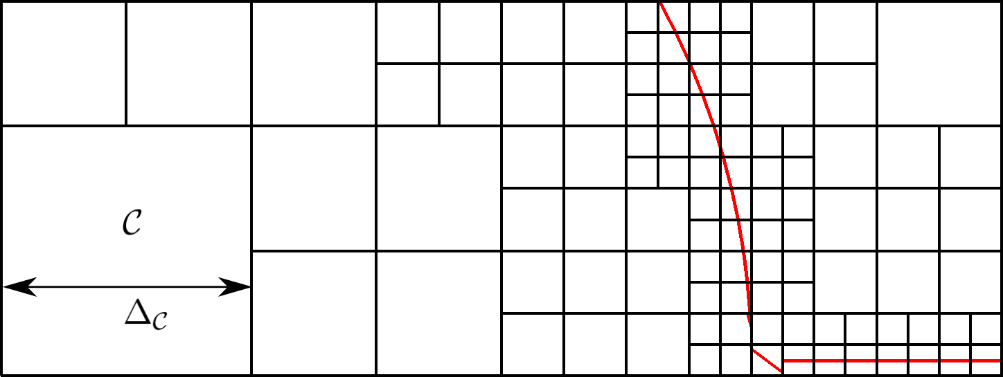
Figure 1: Illustration of the quad-tree used to discretize the continuity domain. The mesh resolution can be chosen adaptively, so that each cell $\mathcal{C}$ has a corresponding size $\Delta_{\mathcal{C}}$. The red curve shows the piecewise linear reconstruction of the liquid/vapor interface obtained using the volume of fluid method.

The system of Eqs. (21)-(22), is solved using the open-source package Gerris [44], described in detail in [18]. In Gerris, the Navier-Stokes equations are solved using a finite-volume based projection method, with the interface between the two fluids tracked using the volume of fluid method. The fluid domain is discretized into a quad-tree of square cells (see Fig. 1); note that we consider the implementation in two spatial dimensions from now onward. The finite-volume method treats each cell $\mathcal{C}$ as a control volume, so that the variables associated with $\mathcal{C}$ represent the volume averaged value of the variable over $\mathcal{C}$. Each cell has a size $\Delta_{\mathcal{C}}$, and center coordinates $(x_{c},y_{c})$. The volume of fluid method tracks the interface implicitly by defining a volume fraction function, $T(\mathcal{C})$, which gives the fraction of the volume of $\mathcal{C}$ occupied by the liquid phase. $T(\mathcal{C})$ is advected by the fluid flow according to the following equation:

$$\partial_{t}T+\nabla\cdot(\textbf{u}T)=0$$ (25)

The value of $We$ and $Ca$ in a cell $\mathcal{C}$ are then represented using an average:

$$We(\mathcal{C}) =We_{l}T(\mathcal{C})+We_{v}(1-T(\mathcal{C}))$$

$$Ca(\mathcal{C}) =Ca_{l}T(\mathcal{C})+Ca_{v}(1-T(\mathcal{C}))$$

Here, as before, subscript $l$ corresponds to liquid, and $v$ to the vapor phase.

The volume of fluid method reconstructs a sharp interface. For each cell, the gradient, $\nabla T$, is computed using the Mixed-Young’s method [45], so that the unit normal vector is given by $\textbf{M}=\nabla T/|\nabla T|$. This permits a linear reconstruction of the interface in each cell, according to the equation $\textbf{M}\cdot\textbf{x}=\alpha$, where $\alpha$ is determined by $T$ (see [46] for details).

The exact average of the force over the computational cell, $\mathcal{C}$, is given by:

$$\textbf{F}_{B}(\mathcal{C})=\frac{1}{\Delta_{C}^{2}}\int\int_{\mathcal{C}}K(\chi(x,y))\mathcal{F}(y)d\mathcal{C}\,\hat{y}\\ =\frac{1}{\Delta_{C}^{2}}\int\int_{\mathcal{C}}\left[K_{ls}\chi(x,y)+K_{vs}(1-\chi(x,y))\right]\mathcal{F}(y)d\mathcal{C}\,\hat{y}$$ (26)

where $\mathcal{F}(y)$ is defined by Eq. (23). We detail two possibilities for the discretization of the van der Waals force term in Eq. (21). For both of these methods, the force is included explicitly in the predictor step of the projection method.

Method I:

Our first method proceeds by a simple second order discretization of Eq. (26):

$$\begin{split}\textbf{F}_{I}(\mathcal{C})&=\frac{\mathcal{F}(y_{c})}{\Delta_{C}^{2}}\int\int_{\mathcal{C}}\left[K_{ls}\chi(x,y)+K_{vs}(1-\chi(x,y))\right]d\mathcal{C}\,\hat{y}\\ &=\left[\frac{\mathcal{F}(y_{c})}{\Delta_{C}^{2}}K_{ls}\int\int_{\mathcal{C}}\chi(x,y)d\mathcal{C}+\frac{\mathcal{F}(y_{c})}{\Delta_{C}^{2}}K_{vs}\int\int_{\mathcal{C}}(1-\chi(x,y))d\mathcal{C}\right]\,\hat{y}\\ \end{split}$$

We identify the average of $\chi$ over $\mathcal{C}$ with $T(\mathcal{C})$, yielding the following expression:

$$\textbf{F}_{I}(\mathcal{C})=\left[T(\mathcal{C})K_{ls}+(1-T(\mathcal{C}))K_{vs}\right]\mathcal{F}(y_{c})\,\hat{y}$$ (27)

However, we note that the accuracy of this simple method can deteriorate at low mesh resolutions because $\mathcal{F}$ has a large gradient as $y\rightarrow 0$. Consider a cell such that $T(\mathcal{C})=1$. To a first approximation, the error in Eq. (27) is given by:

$$\mathcal{E}=|\textbf{F}_{B}(\mathcal{C})-\textbf{F}_{I}(\mathcal{C})|=\left|K_{ls}\frac{\Delta_{C}^{2}}{24}\mathcal{F}^{\prime\prime}(y_{c})+o(\Delta_{C}^{2})\right|\\ \approx\frac{\Delta_{C}^{2}}{24}\frac{K_{ls}}{{h^{\ast}}^{2}}\left|m(m+1)(m+2)\left(\frac{h^{\ast}}{y}\right)^{m+3}\right.\\ \left.-n(n+1)(n+2)\left(\frac{h^{\ast}}{y}\right)^{n+3}\right|$$

To show that this can lead to large errors, consider the error when $\Delta_{\mathcal{C}}=h^{\ast}-h_{c}$, in a cell with center at $y_{c}=(h^{\ast}+h_{c})/2$, i.e. for a cell along the bottom boundary when $h^{\ast}$ is just barely resolved. The error in this cell is:

$$\mathcal{E}_{1}=\frac{(1-h_{c}/h^{\ast})^{2}}{24}K_{ls}\left|m(m+1)(m+2)\left(\frac{2}{1+h_{c}/h^{\ast}}\right)^{m+3}\right.\\ \left.-n(n+1)(n+2)\left(\frac{2}{1+h_{c}/h^{\ast}}\right)^{n+3}\right|$$

The lower bound of this error can be shown to be:

$$\mathcal{E}_{1}>\frac{(1-h_{c}/h^{\ast})^{2}}{24}K_{ls}\left(m(m+1)(m+2)-n(n+1)(n+2)\right)$$

Since $m\geq n+1$, we can bound this further by:

$$\mathcal{E}_{1}>\frac{(1-h_{c}/h^{\ast})^{2}}{8}K_{ls}m(m+1)$$ (28)

Note that $\mathcal{E}_{1}$ is not the discretization error, but the error found for a fixed grid size.

Recalling that Eq. (24) implies that $K_{ls}$ is proportional to $1/{(h^{\ast})}^{2}$, so if $h_{c}$ is significantly smaller than $h^{\ast}$ the errors are quite large unless $\Delta_{C}$ is much smaller than $h^{\ast}$. Furthermore, $h^{\ast}$ is generally small relative to the length scale of the droplet considered in Eq. (13), so that the mesh size required to accurately resolve the right hand side of Eq. (26) will increase the computational cost.

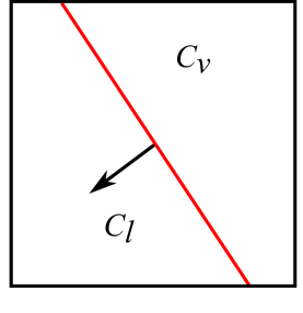
(a)

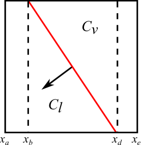
(b)

Figure 2: Illustration of a cell with $0<T(\mathcal{C})<1$: (a) cut cell divided into regions $C_{l}$ and $C_{v}$ entirely occupied by the liquid and vapor phases, respectively, and (b) illustration of the regions of integration of a cut cell. The linear reconstruction of the interface from the volume of fluid method is shown by the red line.

Method II:

Since Eq. (23) gives an exact formula for the force per unit volume in a single phase, much of the simplification used in deriving Eq. (27) is unnecessary. For the second method, we take advantage of this fact to more accurately approximate Eq. (26). First, note that it is trivial to integrate Eq. (26) when $T(\mathcal{C})=1$ or $T(\mathcal{C})=0$. Moreover, the volume of fluid method gives additional information beyond just the fraction of the cell occupied by the liquid phase; using the reconstructed interface, we have an approximation of the portion of the cell which is occupied by the liquid phase as well. Therefore, we introduce the following alternative method. Consider a cell $\mathcal{C}$ with center $(x_{c},y_{c})$, where $0<T(\mathcal{C})<1$, so that the volume of fluid method yields a linear reconstruction of the interface in the cell. This interface divides the cell into a region occupied by the liquid phase, $C_{l}$, and a region occupied by the vapor phase, $C_{v}$ (see Fig. 2(a)). We can write a general algorithm to integrate over these regions, yielding the following expression for the average force on cell $\mathcal{C}$:

$$\textbf{F}_{II}(\mathcal{C})=\left[\frac{\mathcal{K}_{ls}}{\Delta_{C}^{2}}\int\int_{C_{l}}\mathcal{F}(y)dxdy+\frac{\mathcal{K}_{vs}}{\Delta_{C}^{2}}\int\int_{C_{v}}\mathcal{F}(y)dxdy\right]\hat{y}$$ (29)

We briefly outline the general process to perform the integrations over $C_{l}$ and $C_{v}$. Let the volume of fluid reconstructed interface in the cell be given by $\textbf{M}\cdot\textbf{x}=\alpha$, where $\textbf{M}=(M_{x},M_{y})$ is a normal pointing into the liquid phase. We only present the problem of integrating over $C_{l}$, since $C_{v}$ involves an analogous procedure. If $|M_{x}|<\xi$, for a small tolerance $\xi$, the interface is approximately horizontal; thus the integration of $\mathcal{F}(y)$ over $C_{l}$ becomes:

$$\frac{1}{\Delta_{C}^{2}}\int\int_{C_{l}}\mathcal{F}(y)dxdy=\frac{1}{\Delta}\int_{y_{c}-\Delta/2}^{y_{c}-\Delta/2+T\Delta}\mathcal{F}(y)dy$$

On the other hand, if $|M_{y}|<\xi$, the interface is approximately vertical, and the integration over $C_{l}$ becomes:

$$\frac{1}{\Delta_{C}^{2}}\int\int_{C_{l}}\mathcal{F}(y)dxdy=\frac{T}{\Delta}\int_{y_{c}-\Delta/2}^{y_{c}+\Delta/2}\mathcal{F}(y)dy$$

We can now proceed to provide general formulas when $|M_{y}|>\xi$ and $|M_{x}|>\xi$. Since $\mathcal{F}(y)$ is independent of $x$, the sign of the interfacial slope is irrelevant, so, without loss of generality, suppose that $M_{x}/M_{y}>0$. Define the following values:

$$x_{a} =x_{c}-\Delta_{C}/2$$

$$x_{b} =\max\left(\frac{-M_{y}(y_{c}+\Delta_{C}/2)+\alpha}{M_{x}},x_{c}-\Delta_{C}/2\right)$$

$$x_{d} =\min\left(\frac{-M_{y}(y_{c}-\Delta_{C}/2)+\alpha}{M_{x}},x_{c}+\Delta_{C}/2\right)$$

$$x_{e} =x_{c}+\Delta_{C}/2$$

If $M_{y}<0$, the integration over $C_{l}$ can be expressed as follows:

$$\frac{1}{\Delta_{C}^{2}}\int\int_{C_{l}}\mathcal{F}(y)dxdy=\\ \frac{1}{\Delta_{C}^{2}}\left[(x_{b}-x_{a})\int_{y_{c}-\Delta/2}^{y_{c}+\Delta/2}\mathcal{F}dy+\int_{x_{b}}^{x_{d}}\int_{y_{c}-\Delta/2}^{-M_{x}/M_{y}x+\alpha/M_{y}}\mathcal{F}dydx\right]$$ (30)

On the other hand, if $M_{y}>0$, the integration over $C_{l}$ is given by:

$$\frac{1}{\Delta_{C}^{2}}\int\int_{C_{l}}\mathcal{F}(y)dxdy=\\ \frac{1}{\Delta_{C}^{2}}\left[\int_{x_{b}}^{x_{d}}\int_{-M_{x}/M_{y}x+\alpha/M_{y}}^{y_{c}+\Delta/2}\mathcal{F}dydx+(x_{e}-x_{d})\int_{y_{c}-\Delta/2}^{y_{c}+\Delta/2}\mathcal{F}dy\right]$$ (31)

Thus, in two dimensions, the general process of integration reduces to integration over two regions. Note again that $\mathcal{F}(y)$ is known exactly, so that the integrals in Eqs. (30)-(31) can be computed exactly, in contrast to the large error for Method I in Eq. (28). Therefore, we conclude that regarding approximation of Eq. (26), Method II is superior. For example, for a single phase fluid, or when the interface is flat, Eq. (29) is exact. We will consider both Method I and Method II in what follows and discuss their performance.

Our computational domain is rectangular, with $x\in(0,x_{max})$ and $y\in(h_{c},y_{max})$. Throughout the remainder of the paper, we will impose a homogeneous Neumann boundary condition on all boundaries for the pressure, $p$. For the velocity field, we will apply a homogeneous Neumann boundary condition at all boundaries except $y=h_{c}$, where we will apply one of the following two boundary conditions; the no-slip, no-penetration condition by setting ${\bf u}$ to $0$ on the substrate:

$$(u,v)|_{y=h_{c}}=(0,0)$$

or a free-slip condition by:

$$\partial_{y}u|_{y=h_{c}}=0 v|_{y=h_{c}}=0$$

The boundary condition for the van der Waals force is straightforward. At $y=h_{c}$, we set

$$\textbf{F}_{I,II}|_{y=h_{c}}=K_{ls}\mathcal{F}(h_{c})$$

At $y=y_{max}$, we set

$$\textbf{F}_{I,II}|_{y=y_{max}}=K_{vs}\mathcal{F}(y_{max})$$

The boundary condition for the volume fraction, $T$, is again homogeneous Neumann on all boundaries, except on the bottom boundary, where we apply

$$T|_{y=h_{c}}=1$$

which is equivalent to taking the bottom boundary to always be wetted with the liquid phase.

4 Results

In this section, we consider simulations of the full Navier-Stokes equations in which contact angles have been imposed using the van der Waals force, which is included using Methods I and II described in Sec. 3. Our simulation setup consists of a drop on an equilibrium film, initially at rest, which then relaxes to equilibrium under the influence of the van der Waals force. We compare Methods I and II for a drop which is initially close to its equilibrium contact angle, as predicted by Eq. (24), as well as for a spreading drop which is initially far from its equilibrium. Furthermore, we consider the effect of equilibrium film thickness for small, intermediate, and large contact angles, using Method II.

In simulations, droplets are surrounded by an equilibrium film of thickness $\bar{h^{\ast}}:=h^{\ast}-h_{c}$ defined by $y<h^{\ast}$, where $h_{c}$ is the amount the force is translated by in Eq. (17). The initial profile is given by the following:

$$\left\{(x,y):x^{2}+(y+R\cos\theta_{i}-h^{\ast})^{2}<R^{2}\text{ or }y<h^{\ast}\right\}$$ (32)

Here $R$ is chosen so that the total area of the circular cap is equal to $A_{0}=\pi 0.75^{2}/2$. The quantity $\theta_{i}$ is the initial contact angle of the droplet. In all simulations, we fix the ratio of these length scales so that $h^{\ast}=2h_{c}$. Various values of the exponents $m$ and $n$ in Eq. (23) can be found in the literature, in particular $(m,n)=(9,3),~{}(4,3),~{}(3,2)$ have been used in the context of the disjoining pressure in thin films [5, 47], the former corresponding to the 12-6 Lennard Jones potential. In this paper we will restrict our attention to $(m,n)=(3,2)$, which was shown to lead to favorable agreement with experiments involving liquid metal films [47]. Different exponents may affect the structure of the contact line region and the pressure distribution, but do not impact significantly the results presented here.

There are four contact angles that we consider in this section. The initial contact angle, $\theta_{i}$, as in Eq. (32), specifies the angle formed by the tangent of the initial circular profile with the equilibrium film at the point where they meet. The (time dependent) apparent contact angle is denoted $\theta$, and the numerical equilibrium angle $\theta_{num}$ is the value of $\theta$ when the system under consideration is in equilibrium; $\theta$ is measured by a circle fit procedure described below. Finally, we refer to the imposed contact angle, $\theta_{eq}$, which we use to specify $K_{vs}-K_{ls}$ via Eq. (24); the only relevant quantity is the difference between $K_{vs}$ and $K_{ls}$, but for definiteness, we set $K_{vs}=1.1\Delta K(\theta_{eq})$ and $K_{ls}=0.1\Delta K(\theta_{eq})$. The value of $\theta_{eq}$ differs from $\theta_{num}$ in simulations because $h^{\ast}$ is small but non negligible relative to the thickness of the drop.

We measure $\theta$ according to the following procedure. A drop has a circular cap shape that transitions smoothly to the equilibrium film. We define the contact angle in this context in the following way: let $\pm x_{inf}$ represent the points of inflection of the drop profile. We perform a least squares fit of a circle to the profile over the interval $(-x_{inf},x_{inf})$. The point at which the fitted circle intersects the equilibrium film is called the contact point (in three dimensions, this is the contact line). $\theta$ is measured as the angle the fitted circle makes with the equilibrium film at the contact point.

We first investigate a static drop, with $h^{\ast}=0.03$ and $\theta_{i}=\pi/2$, which is then allowed to relax to its equilibrium shape. The dimensionless numbers are set to be $We_{l}=We_{v}=Ca_{l}=Ca_{v}=0.05$. We set the material parameters to be the same in both fluid phases in order to restrict our attention to a smaller parameter space, so that we can focus on the properties of Methods I and II. Note that since the expression determining $\theta_{eq}$, Eq. (24), does not depend on the fluid parameters, this choice does not affect the equilibrium shape. The computational domain is $(x,y)\in[0,2]\times[h_{c},1+h_{c}]$; the domain is resolved at a constant resolution. A no-slip boundary condition is imposed on the solid boundary, $y=h_{c}$.

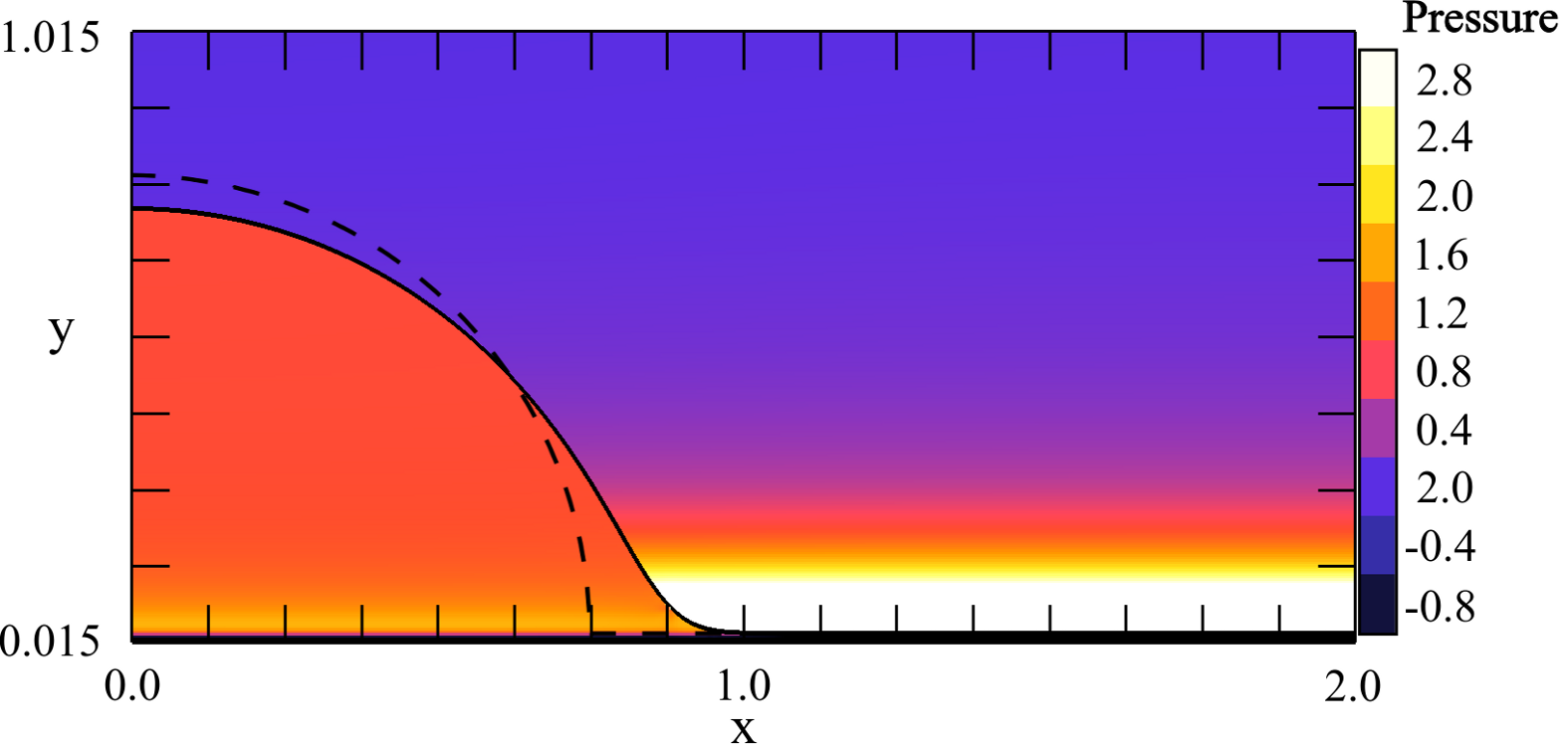
Figure 3: Pressure distribution for a drop with $\theta_{eq}=\pi/2$, $h^{\ast}=0.03$, at equilibrium. The pressure is normalized by the (non-dimensional) capillary pressure of the equilibrium drop, which is given by the curvature of the interface far from the contact point, where it is approximately circular. The solid black curve shows the volume of fluid reconstructed interface, and the dashed curve is the initial profile; $\Delta=1/256$.

Figure 3 shows such a drop at equilibrium (with the contact angle imposed using Method II). The equilibrium film has negative pressure with very high absolute value, and its thickness at equilibrium differs from $\bar{h^{\ast}}$ by about $3\%$. With this $h^{\ast}$, there is a noticeable difference between the true equilibrium contact angle found by simulations, $\theta_{num}$, and the imposed angle $\theta_{eq}$. The effect of $h^{\ast}$ on the equilibrium drop shape will be considered below.

Figure 4 shows the convergence for Methods I and II for a uniform mesh. Simulations are run until time $t=1.75$, with a constant time step of $\Delta t\approx 2.8\times 10^{-5}$; the stability constraint due to the explicit discretization of the surface tension dominates in this velocity regime, and this time step ensures that this constraint is satisfied for all resolutions we consider (see [44]). For two sets of volume fractions $T_{1}$ and $T_{2}$ such that $T_{2}$ is computed on a quad-tree $Q$ with mesh-size $\Delta_{Q}$, the $L^{1}$ norm is computed according to the following formula:

$$||T_{1}(\mathcal{C})-T_{2}(\mathcal{C})||=\sum_{\mathcal{C}\in Q}|T_{1}(\mathcal{C})-T_{2}(\mathcal{C})|\Delta_{Q}^{2}$$ (33)

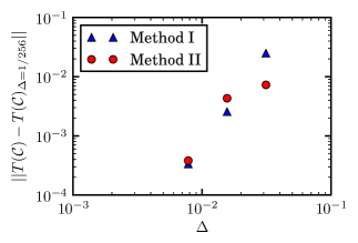
Figure 4: The convergence of the $L^{1}$ norm of the difference between $T(\mathcal{C})$ at $\Delta$ and $\Delta=1/256$, for a drop at equilibrium with $\theta_{eq}=\pi/2$, $h^{\ast}=0.03$, with a uniform mesh size $\Delta$.

In this case $\Delta_{Q}=1/256$, and $T_{1}(\mathcal{C})$ is equal to $T_{1}$ on the largest cell containing $\mathcal{C}$. For reference, $\Delta=1/32$ is about $h^{\ast}$, so that the low resolution case is not even resolving the equilibrium film. Both methods perform comparably well at $\Delta=1/64,1/128$, with Method I converging slightly faster. However, at low resolutions, $\Delta=1/32$, Method II performs significantly better.

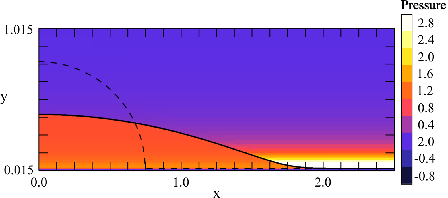
Figure 5: Pressure distribution for a drop at equilibrium with $\theta_{eq}=\pi/6$. Initially, $\theta_{i}=\pi/2$, and the drop spreads to its equilibrium configuration, defined by $\theta_{eq}=\pi/6$. The initial profile is shown by the dashed curve. As in Fig. 3, the pressure is normalized by the capillary pressure of the equilibrium drop; $\Delta=1/256$.

(a) Method I

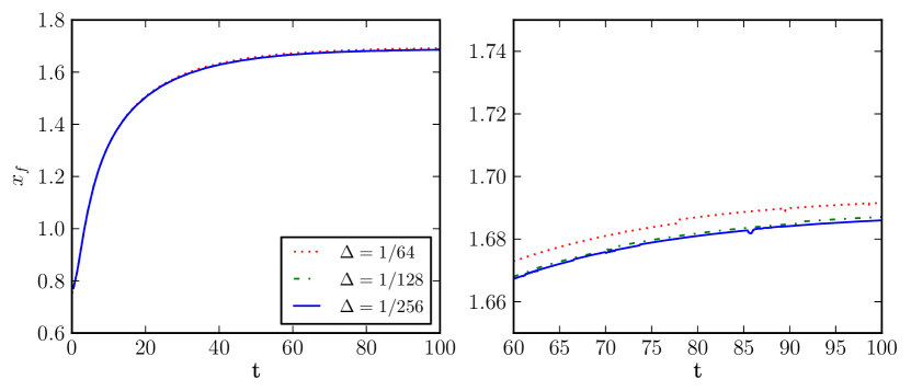
(b) Method II

Figure 6: Front location for the spreading drop for varying resolution for (a) Methods I and (b) Method II. The maximum mesh resolution is $\Delta_{max}=\Delta$.

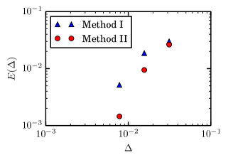
Figure 7: Convergence of the front location of spreading drops, for Methods I and II, where the error is estimated according to Eq. (34).

We now move onto the question of how a drop behaves when $\theta_{i}$ is far from $\theta_{num}$. The initial shape of the drop is as above, with $h^{\ast}=0.03$, $R=0.75$, so that $\theta_{i}=\pi/2$. At $y=h_{c}$, we use free-slip since it allows the drop to reach its steady state more quickly, reducing computational time. The simulation domain is $(x,y)\in[0,4]\times[h_{c},1+h_{c}]$. For these simulations, we will set $We_{l}=We_{v}=Ca_{l}=Ca_{v}=1$. We note that even with this choice of parameters, the dimensionless contact point speed is sufficiently small so that surface tension effects still dominate over viscous effects (or precisely speaking, the capillary number defined based on the speed of the contact point is still small). As before, we use the same material parameters for both phases, and note that, provided that the capillary number is small, varying the ratios between the phases will only affect the relaxation time; we will expand on this point below. Here, we impose a small contact angle of $\theta_{eq}=\pi/6$. Unlike the above, we use an adaptive mesh which refines regions to a level of $\Delta_{max}$ near the liquid/vapor interface, or if there is a high gradient in $\textbf{F}_{B}$. We will vary $\Delta_{max}$ in what follows to study the convergence with respect to the maximum resolution. Figure 5 shows the initial and equilibrium profiles and pressure distribution when the drop reaches equilibrium, computed using Method II. The pressure inside the liquid phase is near unity, while the pressure in the vapor phase just above the equilibrium film is five times the capillary pressure. The equilibrium contact angle in Fig. 5 is $\theta_{num}\approx\pi/7$.

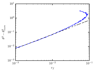
Figure 8: Cox-Voinov law for the spreading drop. The blue (solid) curve shows simulation results for a droplet spreading from $\theta_{i}=\pi/2$ to equilibrium, with an imposed contact angle of $\theta_{eq}=\pi/6$ using Method II. The black (dashed) line is proportional to $v_{f}$, and the agreement with the blue (solid) curve shows that the drop spreading approximately satisfies the Cox-Voinov law.

Figure 6 shows the front locations for the spreading drops as a function of time for Method I and Method II. Both methods show broadly similar results, with Method II appearing to slightly outperform Method I in terms of convergence. In order to compute the convergence, we calculate the error as:

$$E(\Delta)_{I,II}=\frac{1}{100}\int_{0}^{100}|{x_{f}(t)}_{\Delta}-{x_{f}(t)}_{\Delta=1/256}|dt$$ (34)

Here ${x_{f}(t)}_{\Delta}$ is the front location computed with $\Delta_{max}=\Delta$, and ${x_{f}(t)}_{\Delta=1/256}$ is the front location computed with $\Delta_{max}=1/256$. Figure  7 shows the errors. Method II displays significantly better convergence for the front location as a function of time.

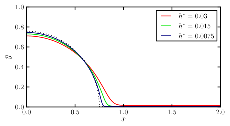
Figure 9: Equilibrium profiles with $\theta_{eq}=\theta_{i}=\pi/2$ for various values of $h^{\ast}$. The black (dotted) profile shows the initial condition for $h^{\ast}=0.015$. We plot $\bar{y}=y-h_{c}$ so that for each curve the $y$ range is $(0,1)$.

We briefly compare the qualitative behavior of the spreading drop to the well known Cox-Voinov law [40]. For a drop displacing another immiscible fluid on a solid surface, the speed of the contact point, $v_{f}$, is related to $\theta_{i}$ and $\theta_{num}$ to leading order by [48]:

$$\theta^{3}-\theta_{num}^{3}\propto v_{f}$$ (35)

Note that Eq. (35) is derived under the assumption that $\mu_{l}v_{f}/\sigma\ll 1$, i.e. that the capillary number defined using the front velocity is small. Provided that one is in this regime, the choice of material parameters only impacts the constant of proportionality in Eq. (35). Figure 8 shows $v_{f}$ versus $\theta^{3}-\theta_{num}^{3}$ using Method II, for $\Delta_{max}=1/256$. The blue (solid) line shows the numerical results, and the black (dashed) line shows the slope expected if the Cox-Voinov law is obeyed. We see that after initial transients $v_{f}$ decreases with $\theta^{3}-\theta_{num}^{3}$, and the drop spreading approximately satisfies the Cox-Voinov law for $v_{f}\in(10^{-2},10^{-3})$.

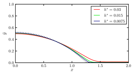
(a)

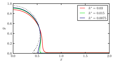
(b)

Figure 10: Dependence of the drop profile at equilibrium on $h^{\ast}$ for (a) $\theta_{eq}=\pi/4$ and (b) $\theta_{eq}=3\pi/4$. The black (dotted) profile shows the initial condition for $h^{\ast}=0.015$. As in Fig. 9, we plot $\bar{y}=y-h_{c}$ so that for each curve the $y$ range is $(0,1)$.

Next, we turn our attention to the precise value of the contact angle. As shown in Figs. 3 and 5, the actual equilibrium contact angle, $\theta_{num}$, is generally smaller than the imposed angle $\theta_{eq}$. This is due to the fact that Eq. (24) is derived under the assumption of small $h^{\ast}$, while in our simulations the ratio of drop radius and $h^{\ast}$ is about 25. To confirm the above statement, we analyze in more detail the resulting contact angles as $h^{*}$ is varied. We set $\theta_{eq}=\pi/2$ using Method II, and the resolution is fixed at a uniform $\Delta=1/256$. The value of $h^{\ast}$ varies over $0.03$, $0.015$, and $0.0075$. The initial condition is imposed with $\theta_{i}=\pi/2$ as in Eq. (32). The drop is again permitted to relax to its equilibrium with a fixed time step for 1.75 units of time. Figure 9 shows the equilibrium profiles for various values of $h^{\ast}$. The black (dotted) profile is the initial condition for $h^{\ast}=0.015$, and is included as a reference. As $h^{\ast}$ is decreased, the equilibrium profiles are characterized by contact angles closer to $\theta_{eq}$.

$h^{\ast}$	$\theta_{num}$	$|\theta_{num}-\theta_{eq}|/{\theta_{eq}}$	$||T_{i}(\mathcal{C})-T_{f}(\mathcal{C})||$
0.03	1.37	0.125	0.05
0.015	1.47	0.066	0.03
0.0075	1.53	0.025	0.009

Table 1: Dependence of $\theta_{num}$ on $h^{\ast}$. We calculate $\theta_{num}$ using a circle fit. The third column gives the relative difference between $\theta_{num}$ and $\theta_{eq}$. The fourth column is the $L^{1}$ norm of the difference between the initial volume fractions $T_{i}(\mathcal{C})$ and the equilibrium $T_{f}(\mathcal{C})$.

We quantify the dependence of $\theta_{num}$ on $h^{\ast}$ in Table 1. As before, we compute the contact angle $\theta_{num}$ using a circle fit of the drop after $1.75$ units of time, at a fixed time step for all simulations. As $h^{\ast}$ is reduced, the calculated $\theta_{num}$ approaches $\theta_{eq}=\pi/2$. The relative difference between $\theta_{num}$ and $\theta_{eq}$ reduces with $h^{\ast}$ approximately linearly. These measures however depend on the accuracy of the estimation of $\theta_{num}$; to analyze the convergence more directly, we compare the volume fractions of the initial condition, $T_{i}(\mathcal{C})$, with the equilibrium state $T_{f}(\mathcal{C})$, using an $L^{1}$ norm computed as Eq. (33). Initially, $\theta_{i}=\theta_{eq}$, so this comparison provides a measure of the difference between $\theta_{num}$ and $\theta_{eq}$. This difference again decreases approximately linearly with $h^{*}$.

Finally, we consider the effects of varying $h^{\ast}$ for $\theta_{eq}$ other than $\pi/2$. Figure 10(a) shows the equilibrium drop profiles for $\theta_{eq}=\theta_{i}=\pi/4$ and varying $h^{\ast}$, and Fig. 10(b) shows the same for $\theta_{eq}=\theta_{i}=3\pi/4$. For $\theta_{eq}=\pi/4$, as $h^{\ast}$ decreases, the profile quickly converges to the initial condition and hence the contact angle to $\theta_{eq}$, as seen by the comparison of the black (dotted) curve with that of $h^{\ast}=0.0075$ in Fig. 10(a). For $\theta_{eq}=3\pi/4$, it can be seen that even for $h^{\ast}=0.0075$, the drop profile still shows some difference between $\theta_{num}$ and $\theta_{eq}$. Nonetheless, this plot demonstrates a central advantage of our methods: $\theta_{num}$ larger than $\pi/2$ can be simulated with the van der Waals force.

5 Conclusions

In this paper, we have described a novel approach for including the fluid/solid interaction forces, into a direct solver of the Navier-Stokes equations with a volume of fluid interface tracking method. The model does not restrict the contact angles to be small, and therefore, can be used to accurately model wetting and dewetting of fluids on substrates characterized by arbitrary contact angles. We study the problem of a two-dimensional drop on a substrate and compare the results with the Cox-Voinov law for drop spreading. These validations and results illustrate the applicability of our proposed method to model flow problems involving contact lines. Furthermore, our approach has the desirable property of regularizing the viscous stress singularity at a moving contact line since it naturally introduces an equilibrium fluid film.

We have considered two alternative finite-volume discretizations of the van der Waals force term that enters the governing equations to include the fluid/solid interaction forces. These two methods are complementary in terms of their accuracy and the ease of use, and therefore the choice of the method could be governed by the desired features of the results. In particular, Method I discretizations can be straightforwardly extended to the third spatial dimension. However, we have shown that, when implementing Method I, to guarantee accurate results, sufficient spatial resolution of the computational mesh must be used. We also show that Method II does not suffer accuracy deterioration at low mesh resolutions, and is therefore, superior to Method I, and furthermore outperforms Method I for spreading drops at all resolutions, albeit being more involved to implement.

The presented approach opens the door for modeling problems that could not be described so far, in particular dewetting and associated film breakup for fluids characterized by large contact angles. Furthermore, the model allows to study the effects of additional mechanisms, such as inertia. We will consider these problems in future work.

References

References

- [1] L. W. Schwartz, R. R. Eley, Simulation of droplet motion on low-energy and heterogeneous surfaces, J. Colloid Interface Sci. 202 (1998) 173.
- [2] J. Diez, L. Kondic, On the breakup of fluid films of finite and infinite extent, Phys. Fluids 19 (2007) 072107.
- [3] J. Eggers, Contact line motion for partially wetting fluids, Phys. Rev. E 72 (2005) 061605.
- [4] A. Oron, S. H. Davis, S. G. Bankoff, Long-scale evolution of thin liquid films, Rev. Mod. Phys. 69 (1997) 931.
- [5] R. Craster, O. Matar, Dynamics and stability of thin liquid films, Rev. Mod. Phys. 81 (2009) 1131.
- [6] K. Mahady, S. Afkhami, J. Diez, L. Kondic, Comparison of Navier-Stokes simulations with long-wave theory: Study of wetting and dewetting, Phys. Fluids 25 (2013) 112103.
- [7] J. N. Israelachvili, Intermolecular and surface forces, Academic Press, New York, 1992, second edition.
- [8] V. P. Carey, Statistical thermodynamics and microscale thermophysics, The Press Syndicate of the University of Cambridge, Cambridge, 1999.
- [9] B. Derjaguin, L. Landau, Theory of the stability of strongly charged lyophobic sols and of the adhesion of strongly charged particles in solutions of electrolytes, Acta Physico Chemica USSR 14 (1941) 633.
- [10] N. V. Churaev, V. D. Sobolev, Prediction of contact angles on the basis of the Frumkin-Derjaguin approach, Adv. Colloid Interface Sci. 61 (1995) 1.
- [11] T. Baer, R. Cairncross, P. Schunk, R. Rao, P. Sackinger, A finite element method for free surface flows of incompressible fluids in three dimensions. part ii. dynamic wetting lines, Int. J. for Num. Meth. in Fluids 33 (3).
- [12] J. E. Sprittles, Y. D. Shikhmurzaev, Finite element framework for describing dynamic wetting phenomena, Int. J. Numer. Meth. Fluids 68 (2012) 1257.
- [13] J. Sprittles, Y. Shikhmurzaev, Finite element simulation of dynamic wetting flows as an interface formation process, J. Comput. Phys. 233 (2013) 34.
- [14] S. Unverdi, G. Tryggvason, A front-tracking method for viscous, incompressible, multi-fluid flows, J. Comp. Phys. 100 (1992) 25.
- [15] M. Sussman, A. S. Almgren, J. B. Bell, P. Colella, L. H. Howell, M. L. Welcome, An adaptive level set approach for incompressible two-phase flows, J. Comput. Phys. 148 (1999) 81.
- [16] Y. Renardy, M. Renardy, PROST: a parabolic reconstruction of surface tension for the volume-of-fluid method, J. Comput. Phys. 183 (2002) 400.
- [17] M. M. Francois, S. J. Cummins, E. D. Dendy, D. B. Kothe, J. M. Sicilian, M. W. Williams, A balanced-force algorithm for continuous and sharp interfacial surface tension models within a volume tracking framework, J. Comput. Phys. 213 (2006) 141.
- [18] S. Popinet, An accurate adaptive solver for surface-tension-driven interfacial flows, J. Comput. Phys. 228 (2009) 5838.
- [19] S. Afkhami, M. Bussmann, Height functions for applying contact angles to 2D VOF simulations, Int. J. Numer. Meth. Fluids 57 (2008) 453.
- [20] S. Afkhami, M. Bussmann, Height functions for applying contact angles to 3D VOF simulations, Int. J. Numer. Meth. Fluids 61 (2009) 827.
- [21] M. Sussman, A method for overcoming the surface tension time step constraint in multiphase flows II, Int. J. Numer. Meth. Fluids 68 (2012) 1343.
- [22] S. Afkhami, L. Kondic, Numerical simulation of ejected molten metal nanoparticles liquified by laser irradiation: Interplay of geometry and dewetting, Phys. Rev. Lett. 111 (2013) 034501.
- [23] P. D. Spelt, A level-set approach for simulations of flows with multiple moving contact lines with hysteresis, J. Comput. Phys. 207 (2005) 389.
- [24] S. Afkhami, S. Zaleski, M. Bussmann, A mesh-dependent model for applying dynamic contact angles to VOF simulations, J. Comput. Phys. 228 (2009) 5370.
- [25] X. Jiang, A. J. James, Numerical simulation of the head-on collision of two equal-sized drops with van der Waals forces, J. Eng. Math 59 (2007) 99.
- [26] J. Jacqmin, Calculation of two-phase navier-stokes flows using phase field modeling, J. Comp. Phys. 155 (1999) 96.
- [27] J. Jacqmin, Contact-line dynamics of a diffuse fluid interface, J. Fluid Mech. 402 (2000) 57.
- [28] J. Jacqmin, Onset of wetting failure in liquid-liquid systems, J. Fluid Mech. 517 (2004) 209.
- [29] P. Yue, C. Zhou, J. Feng, Sharp-interface limit of the Cahn-–Hilliard model for moving contact lines, J. Fluid Mech. 645 (2010) 279.
- [30] D. Sibley, A. Nold, S. Kalliadasis, Unifying binary fluid diffuse-interface models in the sharp interface limit, J. Fluid Mech. 736 (2013) 5.
- [31] A. J. Briant, A. J. Wagner, J. M. Yeomans, Lattice boltzmann simulations of contact line motion. i. liquid-gas systems, Phys. Rev. E. 69 (2004) 031602.
- [32] T. Lee, L. Liu, Lattice boltzmann simulations of micron-scale drop impact on dry surfaces, J. Comp. Phys. 229 (2010) 8045.
- [33] T. Qian, X.-P. Wang, P. Sheng, Molecular hydrodynamics of the moving contact line in two-phase immiscible flows, Comm. Comput. Phys. 1 (2006) 1.
- [34] T. Nguyen, M. Fuentes-Cabrera, J. Fowlkes, J. Diez, A. González, L. Kondic, P. Rack, Competition between collapse and breakup in nanometer-sized thin rings using molecular dynamics and continuum modeling, Langmuir 28.
- [35] M. Fuentes-Cabrera, B. Rhodes, J. Fowlkes, A. López-Benzanilla, H. Terrones, M. Simpson, P. Rack, Molecular dynamics study of the dewetting of copper on graphite and graphene: Implications for nanoscale self-assembly, Phys. Rev. E 83 (2011) 041603.
- [36] K. Mahady, S. Afkhami, L. Kondic, A reduced pressure volume of fluid method for fluid/solid interaction: contact lines and film rupture in 2D and 3D, (in preparation).
- [37] T. Young, An essay on the cohesion of fluids, Philos. Trans. R. Soc. London 95.
- [38] D. Bonn, J. Eggers, J. Indekeu, J. Meunier, E. Rolley, Wetting and spreading, Rev. Mod. Phys. 81 (2009) 739.
- [39] E. B. Dussan V., On the spreading of liquids on solid surfaces: Static and dynamic contact lines, Annu. Rev. Fluid Mech. 11 (1979) 317.
- [40] O. Voinov, Hydrodynamics of wetting, Fluid Dynamics 11 (1976) 714.
- [41] Y. Shikhmurzaev, Moving contact lines in liquid/liquid/solid systems, J. Fluid Mech. 334 (1997) 211.
- [42] J. Snoeijer, A microscopic view on contact angle selection, Phys. Fluids 20 (2008) 057101.
- [43] J. U. Brackbill, D. B. Kothe, C. Zemach, A continuum method for modeling surface tension, J. Comput. Phys. 100 (1992) 335.
- [44] S. Popinet, The Gerris flow solver, http://gfs.sourceforge.net/, 1.3.2 (2012).
- [45] E. Aulisa, S. Manservisi, R. Scardovelli, S. Zaleski, Interface reconstruction with least-square fit and split Eulerian-Lagrangian advection, J. Comput. Phys. 225 (2007) 2301.
- [46] R. Scardovelli, S. Zaleski, Analytical relations connecting linear interfaces and volume fractions in rectangular grids, J. Comput. Phys. 164 (2000) 228.
- [47] A. G. González, J. A. Diez, Y. Wu, J. Fowlkes, P. Rack, L. Kondic, Instability of Liquid Cu films on a SiO2 Substrate, Langmuir 29 (2013) 9378.
- [48] R. G. Cox, The dynamics of the spreading of liquids on a solid surface. Part 1. Viscous flow, Phys. Fluids 168 (1986) 169.