Quantum field theory on toroidal topology: algebraic structure and applications

Abstract

The development of quantum theory on a torus has a long history, and can be traced back to the 1920s, with the attempts by Nordström, Kaluza and Klein to define a fourth spatial dimension with a finite size, being curved in the form of a torus, such that Einstein and Maxwell equations would be unified. Many developments were carried out considering cosmological problems in association with particles physics, leading to methods that are useful for areas of physics, in which size effects play an important role. This interest in finite size effect systems has been increasing rapidly over the last decades, due principally to experimental improvements. In this review, the foundations of compactified quantum field theory on a torus are presented in a unified way, in order to consider applications in particle and condensed matted physics. The theory on a torus $\Gamma_{D}^{d}=({\mathbb{S}}^{1})^{d}\times{\mathbb{R}}^{D-d}$ is developed from a Lie-group representation and c*-algebra formalisms. As a first application, the quantum field theory at finite temperature, in its real- and imaginary-time versions, is addressed by focussing on its topological structure, the torus $\Gamma_{4}^{1}$. The toroidal quantum-field theory provides the basis for a consistent approach of spontaneous symmetry breaking driven by both temperature and spatial boundaries. Then the superconductivity in films, wires and grains are analyzed, leading to some results that are comparable with experiments. The Casimir effect is studied taking the electromagnetic and Dirac field on a torus. In this case, the method of analysis is based on a generalized Bogoliubov transformation, that separates the Green function into two parts: one is associated with the empty space-time, while the other describes the impact of compactification. This provides a natural procedure for calculating the renormalized energy-momentum tensor. Self interacting four-fermion systems, described by the Gross-Neveu and Nambu-Jona-Lasinio models, are considered. Then finite size effects on the hadronic phase structure are investigated, taking into account density and temperature. As a final application, effects of extra spatial dimensions are addressed, by developing a quantum electrodynamics in a five-dimensional space-time, where the fifth-dimension is compactified on a torus. The formalism, initially developed for particle physics, provides results compatible with other trials of probing the existence of extra-dimensions.

1 Introduction

Over the last decades, due to experimental improvements, there is an increasing interest in physical systems where finite size effects play an important role. This is the case of experiments considering effects of extra spatial dimensions or the dependence of the critical temperature on the size of superconductors in films, wires and grains [1, 2]. Compactification is a basic reason for the existence of the Casimir effect, which, for the electromagnetic field, has been measured with a high accuracy only recently [3, 4, 5, 6, 7]. Another outstanding example of size effects is in the transition of the confined to the deconfined state of matter, in particle physics, giving rise to the phase-transition from hadrons to a plasma of quarks and gluons [8, 9]. These results have motivated the development of formalisms to treat size effects [10, 11, 12, 13, 14, 15, 16, 17, 18], such as the quantum field theory on a torus, with well established perturbative methods [19]. Taking into consideration practical applications, in this review, we present developments for the quantum field theory defined on spaces with topologies $\Gamma_{D}^{d}=({\mathbb{S}}^{1})^{d}\times{\mathbb{R}}^{D-d}$, where $D$ is the dimension of the whole space manifold and $d$ is the number of compactified dimensions on the hyper-torus $({\mathbb{S}}^{1})^{d}$, such that $d\leq D$; these can be time (real or imaginary) and spatial dimensions, describing systems in thermal equilibrium subjected to spatial constraints.

Currently, topologies of this type may be associated with extra dimensions; however this is quite an old idea. Historically, one of the first works exploring the notion that our world might have more than four dimensions was carried out by Nordström [20], as a generalization of the Einstein theory of gravitation to a 5-dimensional space-time. Later on, Kaluza [21] and Klein [22] proposed that the fourth spatial dimension would have a finite size, being curved in the form of a circle. The result is that the equations are separated into sets, one of which describes the Einstein equations and the other is equivalent to Maxwell equations. Geometrically, the extra fifth dimension can be viewed as the circle group U(1), which corresponds to the formulation of the electromagnetic theory as a gauge theory with gauge group U(1). There are many theoretical studies in these directions, in particular in string theory which has been reviewed in other places [23, 24, 25, 26, 27]. The existence of such extra dimensions have not been observed in experiments, although there are several studies considering extra-dimension effects, such as the seminal paper by Randal and Sundrum [14]. This is a way to investigate, for instance, the electroweak transition and baryogenesis, by taking a 5-dimensional space-time, using finite-temperature field theory with a compactified extra dimension [28, 29, 15, 30, 31, 32, 33, 34, 35, 36, 37, 38]. Considering that these extra compactified dimensions are beyond our four-dimensional world, it is reasonable to assume that their presence may give rise to effects at different scales, not just those in the cosmological or high energy physics realm, but also in low energy phenomena [39, 40]. With this perspective, effects on the anomalous magnetic moment of the muon, associated with extra-dimensional excitations of the photon and of W and Z bosons, have been studied [41]. Since the $g-2$ experiment at the Brookhaven National Laboratory (USA) in 2004, and subsequent ones, the expected value for $g$ obtained by standard theoretical calculations (that predict $g=2$) could not be confirmed. The reason is that both theoretical predictions and experimental results have a large uncertainty. Although a conclusive response is not available, a value of $g\neq 2$ has not been excluded [42]. In the framework of quantum electrodynamics, a recent experiment for the electron magnetic moment gives a more precise value for $g$: the claimed uncertainty is nearly 6 times lower than in the past. However, there is still a deviation from the value $g=2$ [43]. In atomic physics, very accurate measurements of the asymptotic quantum effects on Rydberg excitations have also been carried out [44]. In this case, another interesting consequence of the possible existence of extra dimensions is that the electric charge may not be exactly conserved; a subject that has been under discussion for a long time [45, 46, 47, 48]. In four-dimensional theories, a very small deviation from electric charge conservation would lead to incompatibilities with low-energy tests of quantum electrodynamics [45]. These inconsistencies can be cured by the introduction of hypothetical millicharged particles [48]. However, this artifact would not be necessary if our world were considered as a submanifold of a higher-dimensional space [45]. From a theoretical point of view, in short, many of these studies, with compactified extra-dimensions, lie in the framework of topologies $\Gamma_{D}^{d}$ [49, 50, 51, 52, 53].

This concept of compactification is not restricted to the discussion of extra-dimensions. An important development, which has its roots in the late fifties, is the first systematic approach to quantum field theory at finite temperature: the imaginary-time (Matsubara) formalism [54]. A fundamental aspect of this method is that it relies on the periodicity (antiperiodicity) of the correlation functions of bosons (fermions) [55, 56, 57, 58]. This periodicity in imaginary-time approach is equivalent to formulating the theory in a compactified torus ${\mathbb{S}}^{1}\times{\mathbb{R}}^{D-1}$, where ${\mathbb{S}}^{1}$ is a circumference of length proportional to the inverse of the temperature [23, 24]. The same mathematical apparatus is applied to a field theory compactified in both space and time [59, 60, 61, 62, 63, 64]. It should be mentioned the pioneering contribution by Birrell and Ford [60], who developed a generalization of the Matsubara mechanism to include compactification of space coordinates. These ideas led to numerous other developments that include spontaneous symmetry breaking for field theories on torus, establishing solid aspects on previous attempts to bring together particle physics and cosmology, such as in the concept of topological mass generation [65, 66, 67, 68, 69, 70, 71, 72, 73, 74].

The topological framework to study finite temperature effects and spatial constraints is developed by considering a $D$-dimensional manifold with a topology of the type $\Gamma_{D}^{d}={\mathbb{S}}^{1_{1}}\times{\mathbb{S}}^{1_{2}}\cdots\times{\mathbb{S}}^{1_{d}}\times{\mathbb{R}}^{D-d}$, with ${\mathbb{S}}^{1_{1}}$ corresponding to the compactification of time and $\,{\mathbb{S}}^{1_{2}},\dots,{\mathbb{S}}^{1_{d}}$ referring to the compactification of $d-1$ spatial dimensions. A characteristic of this topological structure is that it leads to modifications of boundary conditions imposed on fields and correlation functions, but it does not modify the local field equations; $i.e$, the topology plays a role on global properties of the system, but not on local ones, which are associated with the invariants of the Lie space-time symmetries [75, 76]. These developments, that also include algebraic and perturbative analysis, make a toroidal quantum field theory attractive for a broad range of applications.

For instance, an analysis of the spontaneous symmetry breaking for scalar field theories at finite temperature with a compactified spatial dimension [77] has been carried out for superconductors [78, 79, 80, 81]. In this case, the Ginzburg-Landau model for phase transitions is generalized. The model is defined on a $3$-dimensional Euclidean space with one, two or three compactified spatial dimensions; the size of which is respectively the thickness of a film, the cross section of a wire or the volume of a grain. The critical temperature is found as a function of these quantities and minimal sizes, sustaining the transition, are determined. Such achievements are in reasonable agreement with experimental results [80, 82].

A similar analysis of the spontaneous symmetry breaking has been considered for four-fermion interacting fields, a model for describing systems in condensed matter physics, such as superconductivity [83] and aspects of graphene defined from a Dirac theory in $(2+1)$ dimensions [84, 85, 86, 87]. In this case, the quantized Hall conductivities, which are identified as the topological (toroidal) TKNN (Thouless, Kohmoto, Nightingale, den Nijs) [88, 89] integers, are also associated with graphene lattice [90]. These are important applications of the toroidal topology that have been explored and revised extensively [91, 92].

Four-fermion interaction is also employed in phenomenological approaches for particle physics. Simple models describing such interaction are the Nambu-Jona-Lasinio model [93, 94] and the Gross-Neveu model [95]. Both have been formulated on a torus, in order to study, as effective theories for quantum chromodynamics, the phase-transition in the confining/deconfining region [96, 97, 98, 99, 100, 79, 101, 102, 103]. Beyond a phase diagram structure, this formalism provides a critical temperature for the confinement/deconfinement transition in accordance with lattice calculations.

Another application of the toroidal quantum field theory is the Casimir effect. As first analyzed by Casimir [104], the vacuum fluctuations of the electromagnetic field confined between two conducting plates with separation $L$ give rise to an attractive force between the plates. The effect has been studied in different geometries, topologies, fields and physical boundary conditions [105, 106, 107, 108, 109, 110, 111, 112, 113, 114, 115]. The investigations are of interest in diverse areas, such as nano-devices in condensed matter physics, the confinement/deconfinement transition in particle physics and cosmological models [3, 4, 5, 105, 108, 109, 110, 116, 117, 118, 119, 120, 121, 122, 123, 124, 125, 126, 127, 128, 63, 129, 130, 131, 132, 133, 134, 135, 136, 137, 138]. Many aspects of the Casimir effect have been analyzed by studying fluctuations of the vacuum of a field theory compactified on a torus. This is, in particular, due to the association of the toroidal topology with the Dirichlet or Neumann boundary conditions [78, 139, 140, 141, 142, 143, 144, 145, 146, 147]. It is important to emphasize the nature of calculations in the local formulation, initiated by Brown and Maclay [148], to derive the energy-momentum tensor of quantum fields: a procedure that leads naturally to standard renormalization scheme associated with the Casimir effect.

Our goal here is to present the theory of the quantum field theory on a torus as a representation theory, focussing on the aforementioned applications. The presentation is organized in the following way. In Section 2, we review some aspects of the quantum field theory at finite temperature, emphasizing its topological structure, the torus $\Gamma_{4}^{1}$, in imaginary- and real-time formalism. These results are generalized, in Section 3, for theories on torus $\Gamma_{D}^{d}$. The algebraic structure of such a theory is analyzed in Section 4. In Section 5, the Casimir effect is reviewed for the electromagnetic and Dirac fields. In Section 6, the notion of spontaneous symmetry breaking is developed for a quantum theory on a torus. These results are used, in Section 7, to analyze superconductivity in films, wires and grains. In Section 8, the Gross-Neveu and the Nambu-Jona-Lasinio model are studied on toroidal topologies. In Section 9, a quantum electrodynamics with an extra-compactified dimension is developed. The final conclusions and additional comments are presented in Section 10.

2 Thermal field theory and toroidal topology

A systematic approach to many-body physics at finite-temperature was initiated by Matsubara [54]. His method is equivalent to a time-axis Wick rotation of a quantum mechanical system, giving rise to what is known as imaginary time formalism. Further developments included the search for mathematical structures, such as geometrical and topological features, and the generalization of the theory for relativistic particles physics, following along the lines of zero temperature quantum field theory [149, 150, 151, 152, 153, 154].

A first generalization of the Matsubara work was carried out by Ezawa, Tomozawa and Umezawa [55], who extended the imaginary-time formalism to quantum field theories. They discovered, in particular, the periodicity (anti-periodicity) condition for correlation functions of boson (fermion) fields; a concept that later became known as the KMS (Kubo, Martin and Schwinger) condition [153, 154]. Kubo introduced this condition in his paper on linear-response theory [57] in quantum statistical mechanics. Later, Martin and Schwinger [56], developing a real-time formalism for thermal systems in a non-equilibrium state [155], used the KMS condition in quantum electrodynamics [56]. These accomplishments were explored further by Kadanoff and Baym [149]. The KMS condition, an acronym coined by Haag, Hugenholtz and Winnink [58], was early identified as a structural mathematical aspect of the quantum field theory at finite temperature, which was in turn associated with the c*-algebra [156, 157, 158, 159].

The imaginary-time quantum field theory has been applied to different areas. For instance, numerous studies using quantum chromodynamics [160] have been carried out in attempts to understand the quark-gluon plasma and the hadronization phase-transition [161]. An important step to this understanding was carried out by Dolan and Jackiw [162], who studied the effective potential of the $\phi^{4}$ theory at finite temperature, developing the concept of spontaneous symmetry-breaking/restoration.

The imaginary-time formalism is restricted to equilibrium systems. However, there are many examples in high energy and condensed matter physics where time dependance is crucial. This has motivated, over the decades, the search for a real-time formalism at finite temperature [163, 164, 165, 166, 167, 168, 169, 170, 171]. One of these real-time methods is the closed-time path formulation initially due to Schwinger [155]. The approach is constructed by following a path in the complex-time plane and important contributions, which deserve to be mentioned, were carried out by Martin and Schwinger [56], Mahanthappa [172], Bakshi and Mahanthappa[173, 174], Keldysh [175], and Kadanoff and Baym [149]. From this procedure an effective doubling of the degrees of freedom emerges, such that Green functions are represented by $2\times 2$ matrices. Actually, such a doubling has been recognized as an intrinsic characteristic of real-time finite-temperature field theories, providing a correct definition for perturbative analysis [153]. This method is called the Schwinger-Keldysh formalism.

The real-time formalism can be derived from a linear-algebra representation theory. Such a theory was first presented by Takahashi and Umezawa [176, 177, 178], and was called Thermofield Dynamics (TFD). As a consequence of the real-time requirement, a doubling is defined in the original Hilbert space of the system, through the algebraic structure called tilde conjugation rules and thermo-algebras. The temperature is then introduced by a Bogoliubov transformation; that is, a rotation in the doubled space. Furthermore, the propagators are $2\times 2$ matrices. From this fact, an algebraic association with the Schwinger-Keldysh method is established [178, 179].

A thermal theory can be also studied by formulating TFD within the framework of $c$*-algebras and thermo-Lie groups, a modular representation of Lie-algebras [180, 181, 182, 183]. This apparatus provides a physical interpretation for the theory, in particular for the doubling [184, 78, 19], and opens several possibilities for the study of thermal effects [185, 186]. These algebraic developments include perturbative schemes and classical representations [177, 187, 188, 189, 190], with applications to a variety of systems [178, 191, 192, 193, 194, 195, 196, 197, 198, 199, 200, 26, 25, 201, 202, 203, 204, 205].

A distinguishing feature of thermal theories is that, due to the KMS condition, the final prescription of the Matsubara or TFD formalism may be regarded as a compactification of the time coordinate. This corresponds to a field theory on the topology $\mathbb{S}^{1}\times\mathbb{R}^{D-1}$, where $\mathbb{S}^{1}$ is a circumference of length $\beta=1/T$, where $T$ is the temperature, describing the time compactification, and $\mathbb{R}^{D-1}$ stands for $D-1$ space-like coordinates. In this section, we review some basic elements of the thermal quantum field theory, emphasizing such topological aspects.

2.1 Imaginary-time formalism

Let us start with the standard definition of the statistical average of an observable $A$, i.e.

$$\langle A\rangle_{\beta}=\text{Tr}[\rho_{\beta}A]=\frac{1}{Z(\beta)}\text{Tr}\ [e^{-\beta H}A],$$ (1)

where $Z(\beta)$, the partition function, is given by $Z(\beta)=$ Tr$\ (e^{-\beta H})$, where $\beta=1/T$, with $T$ being the temperature and $H$ the Hamiltonian. We use natural units, such that $k_{B}=c=\hbar=1$. In this section, for simplicity, we restrict to the boson field.

An important result regarding the nature of the canonical (or the grand canonical) ensemble is the Kubo-Matin-Schwinger (KMS) condition, stating that the statistical average of an operator in the Heisenberg picture, $A_{H}(t)=e^{itH}A(0)e^{-itH}$, is periodic in time with a period given by $i\beta$. This result can be proved directly from the statistical average, i.e.

$$\langle A_{H}(t)\rangle_{\beta}=\frac{1}{Z}\text{Tr}[\text{\ }e^{-\beta H}A_{H}(t)]\equiv\langle A_{H}(t-i\beta)\rangle_{\beta}.$$ (2)

The change in the argument of $A_{H},$ $t\rightarrow t-i\beta,$ is called a Wick rotation of the time axis.

Consider the free Klein-Gordon field defined in a D-dimensional Euclidian space-time, $\mathbb{R}$, with a point given by $x=(x^{0},\mathbf{z})$, where $x^{0}$ stands for the time and $\mathbf{z}=(z^{1},z^{2},...,z^{D-1})$ the space coordinate, and the Green function

$$G_{0}(x-y;\beta)=i\langle T[\phi(x)\phi(y)]\rangle_{\beta}.$$

It satisfies the KMS condition, Eq. (2), i.e.,

$$G_{0}(x-y;\beta)=G_{0}(x-y+i\beta{n}_{0};\beta),$$ (3)

where ${n}_{0}=(1,0,0,0,...)$. The function $G_{0}(x-y;\beta)$ is a solution of the following equation

$$(\square+m^{2})G_{0}(x-y;\beta)=-\delta(\tau_{x}-\tau_{y})\delta(\mathbf{x}-\mathbf{y}),$$ (4)

where $\tau=it,$ such that $\square+m^{2}=-\partial_{\tau}^{2}-\nabla^{2}+m^{2}$, and is given by

$$G_{0}(x-y;\beta)=\frac{-1}{i\beta}\sum_{n}\int\frac{d^{D-1}p}{2\pi^{3}}\frac{e^{-ik_{n}\cdot x}}{k_{n}^{2}-m^{2}+i\varepsilon},$$ (5)

where $k_{n}=(k_{n}^{0},\mathbf{k})$ and $k_{n}^{0}=2\pi n/\beta$ are the Matsubara frequencies. This solution, the thermal Feynman propagator, is a direct consequence of the KMS condition and is unique, since the periodic boundary condition and the Feynman contour are respected.

The normalized generating functions for this Green function is

$$Z_{0}[J\mathbf{;}\beta]=\exp\left[\frac{i}{2}\int d^{D}xd^{D}y\,J(x)G_{0}(x-y;\beta)J(y)\right],$$ (6)

where

$$G_{0}(x-y;\beta)=i\frac{\delta^{2}Z_{0}[J,\beta]}{\delta J(x)\delta J(y)}|_{J=0}.$$

reproducing the basic result of the Gibbs formalism.

Using the notion of spectral function, as discussed by Kadanoff and Baym [149], Dolan and Jackiw [162] managed to write the thermal propagator in a Fourier-integral representation, thus restoring time as a real quantity. The basic result is that the Fourier-series representation, given in Eq. (5), can be rewritten, using analytical continuation and the spectral function, as

$$G_{0}(x-y;\beta)=\int\frac{d^{D}k}{(2\pi)^{D}}e^{-ik(x-y)}\ G_{0}(k;\beta),$$ (7)

where

$$G_{0}(k;\beta)=G_{0}(k)+\ f_{\beta}(k^{0})[G_{0}(k)-G_{0}^{\ast}(k)]$$

and

$$f_{\beta}(k^{0})=\sum\limits_{l_{0}=1}^{\infty}e^{-\beta\omega_{k}l_{0}}=\frac{1}{e^{\beta\omega_{k}}-1}\equiv n(k^{0};\beta),$$

with $n(k^{0};\beta)$ being the boson distribution function at temperature $T$ with $\omega_{k}=k^{0}$. Then we have

$$G_{0}(k;\beta)=\frac{-1}{k^{2}-m^{2}+i\varepsilon}+n(k^{0};\beta)2\pi i\delta(k^{2}-m^{2}).$$

It is important to emphasize the following aspect. The thermal Green function for the free-boson field is given in Eq. (5), satisfying Eq. (4), the Klein-Gordon equation, and the KMS boundary-condition. Since the Klein-Gordon equation expresses an isometry locally in space-time, such results are equivalent to writing the Klein-Gordon field on a toroidal topology $\Gamma_{4}^{1}=\mathbb{S}^{1}\times\mathbb{R}^{D}$, where $\mathbb{S}^{1}$ describes the compactification in the imaginary time coordinate in a circle of circumference $\beta$. This interpretation is valid not only for free-fields, but also for interacting fields. Since the topology maintains the nature of the local interaction, the Feynman diagrams in $\Gamma_{D}^{1}$ theory are the same except by the following redefinition in the expression of the propagators. In other words, the Feynman rules in the momentum space are modified by taking, for the time-like compactified dimension, the integrals in momentum space replaced by sums as

$$\int\frac{dp^{0}}{2\pi}\rightarrow\frac{1}{i\beta}\sum_{n_{0}=-\infty}^{\infty}$$ (8)

with

$$p^{0}\rightarrow p^{n_{0}}=\frac{2\pi n_{0}}{i\beta},$$ (9)

for bosons, and

$$p^{0}\rightarrow p^{n_{0}}=\frac{2\pi(n_{0}+\frac{1}{2})}{i\beta},$$ (10)

for fermions.

2.2 Real-time formalism

There are two versions for a real-time finite-temperature quantum field theory. One was formulated by Schwinger [56, 172, 173, 174] and Keldysh [175], which is based on using a path in the complex time plane [153]. The other is the thermofield dynamics (TFD) proposed by Takahashi and Umezawa [176]. In this case, the thermal theory is constructed on a Hilbert space and thermal effects are introduced by a Bogoliubov transformation [78]. In equilibrium, these two real-time formalisms are the same [179]. We focus here on basic elements of the TFD approach, emphasizing that a real-time formalism is a theory on the topology $\Gamma_{4}^{1}$.

2.2.1 Thermal state in a Hilbert space

For a system in thermal equilibrium, the ensemble average of an operator $A$ is given by $\langle A\rangle_{\beta}=Z^{-1}(\beta){\rm Tr}(e^{-\beta H}A)$. Then considering $H|n\rangle=E_{n}|n\rangle$, with the set $\{|n\rangle\}$ being an orthonormal basis of the Hilbert space, we write $\langle A\rangle_{\beta}=Z^{-1}(\beta)\sum_{n}e^{-\beta E_{n}}\langle n|A|n\rangle$. In TFD this average is written as

$$\langle A\rangle_{\beta}\equiv\langle 0(\beta)|A|0(\beta)\rangle,$$ (11)

where the thermal state $|0(\beta)\rangle$ is given by [178]

$$|0(\beta)\rangle=Z(\beta)^{-1/2}\sum_{n}e^{-\beta\varepsilon_{n}/2}|n,\tilde{n}\rangle,$$

such that a doubling of the Hilbert space is introduced. A vector of the basis is given by $|n,\tilde{m}\rangle=|n\rangle\otimes|\tilde{m}\rangle$, and the operator $A$ acts on non-tilde vectors, i.e.

$$\langle n,\tilde{n}|A|m,\tilde{m}\rangle=\langle n|\otimes\langle\tilde{n}|A|m\rangle\otimes|\tilde{m}\rangle=\langle n|A|m\rangle\langle\tilde{n}|\tilde{m}\rangle=A_{nm}\delta_{nm}.$$

The tilde in a vector $|m,\tilde{m}\rangle$ indicates that $|\tilde{m}\rangle$ is the replica of $|m\rangle,$ with $m$ and $\tilde{m}$ standing for the same number: $m=\tilde{m}.$ This is why we have written $\langle\tilde{n}|\tilde{m}\rangle=\delta_{nm}$, without reference to the tilde in the $\delta_{mn}$. In a vector like $|m,\tilde{n}\rangle,$ the tilde emphasizes the element of the tilde-Hilbert space only. The vector $|0(\beta)\rangle$ is then a pure state, defined in this doubled Hilbert space, but equivalent to a mixed state describing the thermal equilibrium of a system as far as the averages are concerned.

Let us consider the boson oscillator. Neglecting the zero-point energy, the Hamiltonian is

$$H=wa^{\dagger}a.$$

The creation and destruction operators, $a^{\dagger}$ and $a$ respectively, satisfy the algebra

$$[a,a^{\dagger}]=1\,;\;\;[a,a]=[a^{\dagger},a^{\dagger}]=0.$$ (12)

The eigenvalues and eigenstates of $H$ are specified by $H|n\rangle=nw|n\rangle,\ \ \ n=0,1,2,...,$ where $|0\rangle$ is the vacuum state. These states $|n\rangle$ are orthonormal, i.e., $\langle m|n\rangle=\delta_{mn}$, and the number operator, $N=a^{\dagger}a$, is such that $N|n\rangle=n|n\rangle.$ Since $a^{\dagger}$ and $a$ describe bosons, $|n\rangle$ is a state with $n$ bosons. In order to construct the TFD formalism, we have to double degrees of freedom, giving rise to tilde operators as $\tilde{a}^{\dagger}$ and $\tilde{a}$, commuting with non-tilde operators. For the basic algebraic relations, then we have

$$[\tilde{a},\tilde{a}^{\dagger}]=1\,,\text{ \ \ \ }[\tilde{a},\tilde{a}]=[\tilde{a}^{\dagger},\tilde{a}^{\dagger}]=0,$$ (13)

and the algebra for the non-tilde operators, given in Eqs. (12). The other commutation relations are null.

The thermal state $|0(\beta)\rangle$ is

$$|0(\beta)\rangle =\frac{1}{\sqrt{Z(\beta)}}\sum\limits_{n}e^{-n\beta w/2}|n,\tilde{n}\rangle$$

$$=\frac{1}{\sqrt{Z(\beta)}}\sum\limits_{n}e^{-n\beta w/2}\frac{1}{(n!)^{1/2}}\frac{1}{(\tilde{n}!)^{1/2}}(a^{\dagger})^{n}(\tilde{a}^{\dagger})^{n}|0,\tilde{0}\rangle.$$ (14)

It follows that

$$\langle 0(\beta)|0(\beta)\rangle=\frac{1}{Z(\beta)}\sum\limits_{n,m}\langle m,\widetilde{m}|e^{-\beta w(n+m)/2}|n,\tilde{n}\rangle=\frac{1}{Z(\beta)}\sum\limits_{n}e^{-\beta wn}.$$

Using $\langle 0(\beta)|0(\beta)\rangle=1$, we find

$$Z(\beta)=\frac{1}{1-e^{-\beta w}}.$$ (15)

From Eq. (14) we have

$$|0(\beta)\rangle=\sqrt{1-e^{-\beta w}}\sum\limits_{n}\frac{e^{-n\beta w/2}}{n!}(a^{\dagger})^{n}(\tilde{a}^{\dagger})^{n}|0,\tilde{0}\rangle.$$ (16)

In this way we are able to proceed with calculations in statistical mechanics using, instead of the canonical density matrix, the state $|0(\beta)\rangle$. To explore this possibility, Eq. (16) is written in the form $|0(\beta)\rangle=U(\beta)|0,\tilde{0}\rangle,$ where $U(\beta)$ is a unitary operator.

The sum in Eq. (16) is an exponential, i.e

$$|0(\beta)\rangle=\sqrt{1-e^{-\beta w}}\exp(e^{-\beta w/2}a^{\dagger}\tilde{a}^{\dagger})|0,\tilde{0}\rangle.$$ (17)

This result is written as an exponential function only, and as such a unitary operator, by taking into account the operator relation

$$e^{\alpha(A+B)}=e^{\tanh\alpha B}e^{\ln\cosh\alpha C}e^{\tanh\alpha A},$$ (18)

where $C=[A,B]$. Defining

$$\cosh\theta(\beta) =\frac{1}{\sqrt{1-e^{-\beta w}}}\equiv u(\beta),$$ (19)

$$\sinh\theta(\beta) =\frac{e^{-\beta w/2}}{\sqrt{1-e^{-\beta w}}}\equiv v(\beta),$$ (20)

we obtain

$$|0(\beta)\rangle =\cosh^{-1}\theta(\beta)e^{\tanh\theta(\beta)a^{\dagger}\tilde{a}^{\dagger}}|0,\tilde{0}\rangle$$

$$=\exp\left[\tanh\theta a^{\dagger}\tilde{a}^{\dagger}\right]\exp\left[-\ln\cosh\theta(\tilde{a}\tilde{a}^{\dagger}+a^{\dagger}a)\right]\exp\left[\tanh\theta(-\tilde{a}a)\right]|0,\tilde{0}\rangle,$$ (21)

where we have used the commutation relation $[\tilde{a},\tilde{a}^{\dagger}]=1$ and $e^{f(\theta)\tilde{a}^{\dagger}\tilde{a}}|0,\tilde{0}\rangle=|0,\tilde{0}\rangle,$ where $f(\theta)$ is an arbitrary function of $\theta.$

Using the identity given in Eq. (18) with $A=-\tilde{a}a$, $B=a^{\dagger}\tilde{a}^{\dagger}$, $C=[A,B]=-\tilde{a}\tilde{a}^{\dagger}-a^{\dagger}a$, and $\alpha=\theta=\theta(\beta)$, we have

$$|0(\beta)\rangle=e^{-iG(\beta)}|0,\tilde{0}\rangle,$$ (22)

where

$$G(\beta)=-i\theta(\beta)(\tilde{a}a-\tilde{a}^{\dagger}a^{\dagger}).$$ (23)

Hence the unitary operator, transforming $|0,\tilde{0}\rangle$ into $|0(\beta)\rangle,$ is given by

$$U(\beta)=e^{-iG(\beta)}.$$ (24)

This operator $U(\beta)$ defines a Bogoliubov transformation.

Using $U(\beta)$, let us introduce the following thermal operators through the relations

$$a(\beta)=U(\beta)aU^{\dagger}(\beta)\;,\;\;\;\;\;\tilde{a}(\beta)=U(\beta)\tilde{a}U^{\dagger}(\beta).$$

The importance of these operators lies in the fact that $a(\beta)|0(\beta)\rangle=U(\beta)aU^{\dagger}(\beta)U(\beta)|0,\widetilde{0}\rangle=U(\beta)a|0,\tilde{0}\rangle=0,$ and $\tilde{a}(\beta)|0(\beta)\rangle=0.$ Then $|0(\beta)\rangle$ is a vacuum for $a(\beta)$ and $\tilde{a}(\beta)$, but it is not a vacuum for $a$ and $\tilde{a}$. In this sense, $|0(\beta)\rangle$ is a pure state for thermal operators, and a thermal state for non-thermal operators. This is the reason that $|0(\beta)\rangle$ is called a thermal vacuum.

Since $U(\beta)$ is a unitary transformation, the algebra of the original operators $a$ and $\tilde{a}$ is kept invariant, i.e. the operators $a(\beta)$ and $\tilde{a}(\beta)$ satisfy the following commutation relations

$$[a(\beta),a^{\dagger}(\beta)]=1;\,\,\,\,[\tilde{a}(\beta),\tilde{a}^{\dagger}(\beta)]=1,$$ (25)

with all the other commutation relations being zero. Let us consider, as an example, the average of the number operator $N=a^{\dagger}a$. We find that

$$n(\beta) =\langle N\rangle=\langle 0(\beta)|a^{\dagger}a|0(\beta)\rangle$$

$$=\langle 0(\beta)|[u(\beta)a^{\dagger}(\beta)+v(\beta)\tilde{a}(\beta)][u(\beta)a(\beta)+v(\beta)\tilde{a}^{\dagger}(\beta)]|0(\beta)\rangle$$

$$=v^{2}(\beta)=\frac{1}{e^{\beta w}-1},$$ (26)

where we have used $a(\beta)|0(\beta)\rangle=0$ and $\tilde{a}(\beta)|0(\beta)\rangle=0$. This is the boson distribution function for a system in thermal equilibrium.

Using $u^{2}(\beta)-v^{2}(\beta)=1$, we find

$$a^{\dagger}(\beta)a(\beta)-\tilde{a}^{\dagger}(\beta)\tilde{a}(\beta)=a^{\dagger}a-\tilde{a}^{\dagger}\tilde{a}.$$ (27)

This result can be used to determine the form of the generator of time translation, the Hamiltonian $\widehat{H}$ of the theory. Demanding the invariance of $\widehat{H}$ under the Bogoliubov transformation, the simplest form for $\widehat{H}$ is $\widehat{H}=H-\widetilde{H}$, such that

$$\widehat{H}(\beta)=H(\beta)-\widetilde{H}(\beta)=\omega[a^{\dagger}(\beta)a(\beta)-\tilde{a}^{\dagger}(\beta)\tilde{a}(\beta)]=\omega[a^{\dagger}a-\tilde{a}^{\dagger}\tilde{a}]=\widehat{H}.$$

With this expression for $\widehat{H}$, we have all the elements to fix the tilde mapping, i.e., $\widetilde{\ \ \ }:A\rightarrow\widetilde{A}$. We first observe that, the equations of motion, in the Heisenberg picture, for an arbitrary operator $A$ and its partner $\widetilde{A}$ are $i\partial_{t}A(t)=[A(t),\widehat{H}]$ and $i\partial_{t}\widetilde{A}(t)=[\widetilde{A}(t),\widehat{H}]$. This leads to

$$i\partial_{t}A(t) =[A(t),\widetilde{H}]=A(t)H-HA(t)$$

$$-i\partial_{t}\widetilde{A}(t) =[\widetilde{A}(t),\widetilde{H}]=A(t)\widetilde{H}-\widetilde{H}A(t).$$

Comparing these two equations, we conclude the following conditions for the tilde mapping:

$$(A_{i}A_{j})\widetilde{} =\widetilde{A}_{i}\widetilde{A}_{j},$$ (28)

$$(cA_{i}+A_{j})\widetilde{} =c^{\ast}\widetilde{A}_{i}+\widetilde{A}_{j},$$ (29)

$$(A_{i}^{\dagger})\widetilde{} =(\widetilde{A}_{i})^{\dagger},$$ (30)

$$(\widetilde{A}_{i})\widetilde{} =A_{i},$$ (31)

$$[A_{i},\widetilde{A}_{j}] =0.$$ (32)

These properties are called tilde conjugation rules.

The thermal Fock space, $\mathcal{H}_{T}$, is constructed from the vacuum $|0(\beta)\rangle,$ and is spanned by the set of states given by

$$\{\ |0(\beta)\rangle,\ a^{\dagger}(\beta)|0(\beta)\rangle,\ \ \tilde{a}^{\dagger}(\beta)|0(\beta)\rangle,\,\dots\,,\ \frac{1}{\sqrt{n!}}\frac{1}{\sqrt{m!}}\left(a^{\dagger}(\beta)\right)^{n}\left(\tilde{a}^{\dagger}(\beta)\right)^{m}|0(\beta)\rangle\,\dots\}.$$

These states and their superpositions are physically identified since each one corresponds to a density matrix [78]. This is the case of the thermal vacuum, $|0(\beta)\rangle$ that corresponds to the equilibrium density matrix, $\rho_{\beta}$.

A doublet notation is introduced by defining

$$\left(\begin{array}[c]{c}a(\beta)\\ \tilde{a}^{\dagger}(\beta)\end{array}\right)=B(\beta)\left(\begin{array}[c]{c}a\\ \tilde{a}^{\dagger}\end{array}\right),$$ (33)

where

$$B(\beta)=\left(\begin{array}[c]{cc}u(\beta)&-v(\beta)\\ -v(\beta)&u(\beta)\end{array}\right).$$ (34)

Given two arbitrary (boson) operators $A$ and $\widetilde{A},$ a doublet notation is given by

$$\left(A^{a}\right)=\left(\begin{array}[c]{c}A^{1}\\ A^{2}\end{array}\right)=\left(\begin{array}[c]{c}A\\ \widetilde{A}^{\dagger}\end{array}\right),$$ (35)

with a tilde transposition given by

$$(\overline{A}^{a})=(A^{\dagger},-\widetilde{A}).$$ (36)

We now address the problem of a thermal quantum field.

2.2.2 Thermal quantum field in real-time formalism

Using the fact that for a boson oscillator the Hamiltonian is given by $\widehat{H}=H-\widetilde{H}$, we can construct a Lagrangian formalism given by $\widehat{\mathcal{L}}=\mathcal{L-}\widetilde{\mathcal{L}}$. The extension for a field follows along the same lines. Then, for the Klein-Gordon field with an external source we have

$$\widehat{\mathcal{L}}=\mathcal{L-}\widetilde{\mathcal{L}}=\frac{1}{2}\partial_{\alpha}\phi\partial^{\alpha}\phi-\frac{1}{2}m^{2}\phi^{2}+J\phi-\frac{1}{2}\partial_{\alpha}\widetilde{\phi}\partial^{\alpha}\widetilde{\phi}+\frac{1}{2}m^{2}\widetilde{\phi}^{2}-\widetilde{J}\widetilde{\phi}.$$

In order for the Hamiltonian formalism to be derived, we define the canonical momentum density by

$$\pi(x)=\frac{\partial\mathcal{L}(\phi,\partial\phi)}{\partial\dot{\phi}}\;,\;\;\;\;\;\widetilde{\pi}(x)=\frac{\partial\widetilde{\mathcal{L}}(\widetilde{\phi},\partial\widetilde{\phi})}{\partial\dot{\widetilde{\phi}}}.$$

The Hamiltonian is defined by

$$\widehat{H}=\int\widehat{\mathcal{H}}\,d^{3}x=\int[{\mathcal{H}}(\phi,\pi)-\widetilde{\mathcal{H}}(\widetilde{\phi},\widetilde{\pi})]\,d^{3}x,$$ (37)

where the Hamiltonian density is

$$\widehat{\mathcal{H}}=\frac{1}{2}\pi^{2}+\frac{1}{2}(\nabla\phi)^{2}+\frac{1}{2}m^{2}\phi^{2}-J\phi-\frac{1}{2}\widetilde{\pi}^{2}-\frac{1}{2}(\nabla\widetilde{\phi})^{2}-\frac{1}{2}m^{2}\widetilde{\phi}^{2}+\widetilde{J}\widetilde{\phi}.$$

A quantum field theory is introduced by requiring that the equal-time non-zero commutation relations are fulfilled,

$$[\phi(t,\mathbf{x),}\pi(t,\mathbf{y)}] =i\delta(\mathbf{x-y}),$$ (38)

$$[\widetilde{\phi}(t,\mathbf{x),}\widetilde{\pi}(t,\mathbf{y)}] =-i\delta(\mathbf{x-y}),$$ (39)

The fields $\phi$ and $\pi$ are operators defined to act on a Hilbert space $\mathcal{H}_{T}$. We use the Bogoliubov transformation to introduce thermal operators. In this case there are infinite modes and so a Bogoliubov transformation is defined for each mode, i.e.

$$\phi(x;\beta)=\int\frac{d^{3}k}{(2\pi)^{3}}\frac{1}{2\omega_{k}}\ [a(k;\beta)e^{-ikx}+a^{{\dagger}}(k;\beta)e^{ikx}]$$

and

$$\widetilde{\phi}(x;\beta)=\int\frac{d^{3}k}{(2\pi)^{3}}\frac{1}{2\omega_{k}}\ [\tilde{a}(k;\beta)e^{ikx}+\tilde{a}^{{\dagger}}(k;\beta)e^{-ikx}],$$

where $a(k;\beta)$ ($\tilde{a}(k;\beta))$ and $a^{{\dagger}}(k;\beta)$ ($\tilde{a}^{{\dagger}}(k;\beta))$ are thermal (tilde) annihilation and creation operators. For the momenta, $\pi(x;\beta)$ and $\widetilde{\pi}(x;\beta),$ we have

$$\pi(x;\beta)=\dot{\phi}(x;\beta)=\int\frac{d^{3}k}{(2\pi)^{3}}(-i)\ \frac{1}{2}[a(k;\beta)e^{-ikx}-a^{{\dagger}}(k;\beta)e^{ikx}]$$

and

$$\widetilde{\pi}(x;\beta)=\dot{\widetilde{\phi}}(x;\beta)=\int\frac{d^{3}k}{(2\pi)^{3}}\ \frac{i}{2}[\tilde{a}(k;\beta)e^{ikx}-\tilde{a}^{{\dagger}}(k;\beta)e^{-ikx}],$$

where we have used the tilde conjugation rules to write $\widetilde{\phi}(x;\beta)$ and $\widetilde{\pi}(x;\beta)$ from $\phi(x;\beta)$ and $\pi(x;\beta),$ respectively.

The algebra given by Eqs. (38) and (39) is still valid for the operators $\phi(x;\beta),$ $\widetilde{\phi}(x;\beta),\pi(x;\beta)$ and $\widetilde{\pi}(x;\beta).$ Then the commutation relations for the thermal modes read

$$[a(k;\beta),a^{{\dagger}}(k^{\prime};\beta)] =(2\pi)^{3}2k_{0}\delta(\mathbf{k}-\mathbf{k}^{\prime}),$$ (40)

$$[\tilde{a}(k;\beta),\tilde{a}^{{\dagger}}(k^{\prime};\beta)] =(2\pi)^{3}2k_{0}\delta(\mathbf{k}-\mathbf{k}^{\prime}),$$ (41)

with all the other commutation relations being zero. The general Bogoliubov transformation applied to all modes is written in the form

$$U(\beta)=\exp\left\{\sum_{k}\theta_{k}(\beta)[a^{{\dagger}}(k)\tilde{a}^{{\dagger}}(k)-a(k)\tilde{a}(k)]\right\}=\prod_{k}U(k,\beta),$$ (42)

where

$$U(k,\beta)=\exp\{\theta_{k}(\beta)[a^{{\dagger}}(k)\tilde{a}^{{\dagger}}(k)-a(k)\tilde{a}(k)]\},$$

with $\theta_{k}$ defined by $\cosh\theta_{k}=v(k,\beta),$ in the limit of the continuum. However, in this limit the unitary nature of the Bogoliubov transformation is lost, a property that gives rise to non-equivalent vacua in the theory [178]. Despite the loss of unitarity, the Bogoliubov transformation is still canonical, in the sense that, the algebraic structure of the theory is preserved.

The thermal Hilbert space, $\mathcal{H}_{T}$, is constructed from the thermal vacuum, $|0(\beta)\rangle=U(\beta)|0,\tilde{0}\rangle,$ where $|0,\tilde{0}\rangle={\bigotimes}_{k}|0,\tilde{0}\rangle_{k}$ and $|0,\tilde{0}\rangle_{k}$  is the vacuum for the mode $k.$ The thermal vacuum is such that $a(k;\beta)|0(\beta)\rangle=\tilde{a}(k;\beta)|0(\beta)=0$ and $\langle 0(\beta)|0(\beta)\rangle=1$.

The thermal and non-thermal operators are related by

$$a(k;\beta)=U(\beta)a(k)U^{-1}(\beta)=u(k,\beta)a(k)-v(k,\beta)\tilde{a}^{\dagger}(k),$$ (43)

where $v(k,\beta)=1/\sqrt{\exp(\beta\omega_{k})-1}$ and $u^{2}(k,\beta)-v^{2}(k,\beta)=1$. The other operators, $a^{\dagger}(k),$ $\tilde{a}(k)$ and $\tilde{a}^{\dagger}(k)$ are derived by using the Hermitian and the tilde conjugation rules.

The thermal Feynman propagator for the real scalar field is then defined by

$$G(x-y;\beta)^{ab}=-i\langle 0(\beta)|T[{\Phi}(x)^{a}{\Phi}^{+}(y;\beta)^{b}]|0(\beta)\rangle=\frac{1}{(2\pi)^{4}}\int d^{4}k\,G(k;\beta)^{ab}e^{-ik(x-y)},$$ (44)

where $a,b=1,2$, with $a=1$ standing for non-tilde operators and $a=2$ standing for tilde operators; $G(k;\beta)^{ab}=B^{-1}(k_{0};\beta)G_{0}(k)^{ab}B(k_{0};\beta),$ with

$$(G_{0}(k)^{ab})=\left(\begin{array}[c]{cc}\frac{1}{k^{2}-m^{2}+i\epsilon}&0\\ 0&\frac{-1}{k^{2}-m^{2}-i\epsilon}\end{array}\right),$$ (45)

such that the components of $G(k;\beta)^{ab}$ are given by

$$G(k;\beta)^{11} =\frac{1}{k^{2}-m^{2}+i\epsilon}-2\pi i\,n(k_{0})\,\delta(k^{2}-m^{2}),$$

$$G(k;\beta)^{22} =\frac{-1}{k^{2}-m^{2}-i\epsilon}-2\pi i\,n(k_{0})\,\delta(k^{2}-m^{2}),$$

$$G(k;\beta)^{12} =G(k;\beta)^{21}=-2\pi i\,[n(k_{0})+n(k_{0})^{2}]^{1/2}\,\delta(k^{2}-m^{2}),$$

where $n(k_{0})=v_{k}(\beta)^{2}$. The propagator $G(k;\beta)^{11}$ is the same as in the Fourier integral representation of the Matsubara method; and the two-by-two Green function in Eq. (44) is similar to the propagator in the Schwinger-Keldysh approach.

Closing this section, let us emphasize some aspects of the real time formalism. First, it is important to note that doubling is not a characteristic of TFD only, but rather an ingredient present in any thermal theory. In terms of the density matrix, the doubling is needed when we write $\rho(t)$ as a projector, i.e. $\rho\simeq|\psi\rangle\langle\psi|$, and the Liouville von-Neumann equation is written in the form $i\partial_{t}\rho(t)=L\rho(t).$ In this later case, the time evolution is controlled by $L=[H,.\,]$, the Liouvilian, which is an object associated with, but different from, the Hamiltonian operator, $H$. In TFD as in the density matrix formalism, this doubling has been physically identified and plays a central role in the construction of mixed states, for instance. Another aspect to be emphasized is that a real-time formalism is also a theory on $\Gamma_{4}^{1}$ topology, where the state $|0(\beta)\rangle$ is the counterpart ingredient of the imaginary-time procedure. The generalization of the thermal theory, in both versions of Fourier series representation or the integral representation, leads naturally to a theory on $\Gamma_{D}^{d}$ topology. These aspects are explored in the next section.

As a final observation, it is to be noted that the TFD structure has been described in geometric terms. Indeed, Israel showed that one can observe a thermal vacuum for particle modes limited by a space-time horizon [206]. The procedure was a geometric description of TFD, which generalized the results of Fulling, Gibbons, Hawking and Unruh about black holes. These ideas were improved in several directions, using Rindler coordinates and the notion of entanglement of the left and right Rindler quanta [207, 208, 209].

3 Field theory on the topology $\Gamma_{D}^{d}$

In this section, we generalize the argument advanced in the previous section establishing that a quantum field theory at finite temperature corresponds to a field theory on a topology $\Gamma_{D}^{1}=(\mathbb{S}^{1})\times\mathbb{R}^{D-1}$, where the imaginary time is the compactified dimension. We proceed further with these concepts, to include in the analysis not only time but also space coordinates, in such way that any set of dimensions of the manifold $\mathbb{R}^{D}$ can be compactified, defining a theory on the topology $\Gamma_{D}^{d}=(\mathbb{S}^{1})^{d}\times\mathbb{R}^{D-d}$, with $1\leq d\leq D$. This establishes a formalism that suffices to deal with the general question of compactification on the $\Gamma_{D}^{d}$ topology at finite-temperature, in the imaginary or real time [60, 61, 184, 78, 19].

Using a generalized Bogoliubov transformation, the effect of compactification on $\Gamma_{D}^{d}$ is introduced and a Fourier integral representation for the propagator is derived. Initially, an analysis is carried out for free boson and fermion fields. An extension of the formalism for abelian and non-abelian gauge-fields is derived by functional methods. Exploring the canonical formalism, the S-matrix is developed [184, 78, 19].

3.1 Generalized Matsubara procedure

We consider a D-dimensional space-time, $\mathbb{R}$, with a point given by $x=(x^{0},\mathbf{z})$, where $x^{0}$ stands for the time and $\mathbf{z}=(z^{1},z^{2},...,z^{D-1})$ space coordinates. Since the toroidal topology keeps the nature of the local interaction, the Feynman rules for a field theory on the hyper-torus $\Gamma_{D}^{d}$ are a generalization of the Matsubara prescription, Eqs. (8)-(10). Explicitly, the Feynman rules in the momentum space are modified by taking, for each compactified space dimension, the integrals in momentum space replaced by sums, in the following way:

$$\int\frac{dp^{i}}{2\pi}\rightarrow\frac{1}{L_{i}}\sum_{l_{i}=-\infty}^{\infty}$$

with $i=1,...,D-1$,

$$p_{i}\rightarrow p_{l_{i}}=\frac{2\pi l_{i}}{L_{i}},$$

for bosons, and

$$p_{i}\rightarrow p_{l_{i}}=\frac{2\pi(l_{i}+\frac{1}{2})}{L_{i}},$$

for fermions .

For a free boson field compactified in $d\leq D$ dimensions, satisfying periodic boundary condition, we have

$$G_{0}(x-x^{\prime};\alpha)=\frac{1}{i^{d}\,\alpha_{0}\cdot\cdot\cdot\alpha_{d-1}}\sum\limits_{n_{0}\cdot\cdot\cdot n_{d-1}}\int\frac{d^{D-d}\mathbf{k}}{(2\pi)^{D-d}}\,\frac{e^{-ik_{\alpha}(x-x^{\prime})}}{k_{\alpha}^{2}-m^{2}+i\varepsilon},$$ (46)

where $k_{\alpha}=(k_{n_{0}}^{0},k_{n_{1}}^{1},\dots,k_{n_{d-1}}^{d-1},k^{d},\dots,k^{D-1})$, with

$$k_{n_{j}}^{j}=\frac{2\pi n_{j}}{\alpha_{j}},\ \ 0\leq j\leq d-1,$$

$n_{j}\in\mathbb{Z}$ and $d^{D-d}\mathbf{k}=dk^{d}dk^{d+1}\cdots dk^{D-1}$. The compactification parameters $\alpha=(\alpha_{0},\alpha_{1},...,\alpha_{D})$ stand for the effect of temperature ($\alpha_{0}=\beta=T^{-1}$) and for space compactifion ($\alpha_{j}$). In what follows, we employ the name Matsubara representation (or prescription) referring to both time and space compactification. The Green function $G_{0}(x-x^{\prime};\alpha)$ is a solution of the Klein-Gordon equation. This means that $G_{0}(x-x^{\prime};\alpha)$ is the Green function of a boson field defined locally in the Minskowki space-time. Globally this theory is such that $G_{0}(x-x^{\prime};\alpha)$ has to satisfy periodic boundary conditions (the generalization of the KMS condition). These facts assure us that $G_{0}(x-x^{\prime};\alpha)$ is the Green function of a field theory defined on a hyper-torus, $\Gamma_{D}^{d}=(\mathbb{S}^{1})^{d}\times\mathbb{R}^{D-d}$, with $1\leq d\leq D$, where the circumference of the $j$-th $\mathbb{S}^{1}$ is specified by $\alpha_{j}$.

We proceed to study representations in terms of the spectral function, as derived for the case of temperature by Dolan and Jackiw [162]. For the case of compactified spatial dimensions, the spectral function is defined in terms of the momentum, such that the calculation follows in parallel with the case of temperature. At the end of the calculation a Wick rotation is performed in order to recover the physical meaning of the theory [19]. We start, for simplicity, with one-compactified dimension. Take the topology $\Gamma_{D}^{1}$ where the imaginary time-axis is compactified. In this case, we denote, $\alpha=(\beta,0,\dots,0)=\beta n_{0}$, $n_{0}=(1,0,\dots,0)$, with $T=\beta^{-1}$ being the temperature, such that the Green function is given by Eq. (5) and its Fourier integral representation is given in Eq. (7). In the case of compactification of the coordinate $x^{1}$, for the topology $\Gamma_{D}^{1}$, we take $\alpha=(0,iL_{1},0,\dots,0)=iL_{1}n_{1}$, with $n_{1}=(0,1,0,\dots,0)$. The factor $i$ in the parameter $\alpha_{j}$ corresponding to the compactification of a space coordinate makes explicit that we are working with the Minkowski metric; the period in the $x^{1}$ direction is real and equal to $L_{1}$. The propagator has the Matsubara representation

$$G_{0}(x-y;L_{1})=\frac{1}{L_{1}}\sum\limits_{l_{1}}\int\frac{d^{D-1}\mathbf{k}}{(2\pi)^{D-1}}\frac{e^{-ik_{l_{1}}(x-y)}}{(k_{l_{1}})^{2}-m^{2}+i\varepsilon},$$

where $k_{l_{1}}=(k^{0},k_{l_{1}}^{1},k^{2},\dots,k^{D-1})$, with $k_{l_{1}}^{1}=2\pi l_{1}/L_{1}$. The Fourier-integral representation is derived along the same way as for temperature [19], leading to

$$G_{0}(x-y;L_{1})=\int\frac{d^{D}k}{(2\pi)^{D}}e^{-ik(x-y)}\ G_{0}(k;L_{1}),$$

where

$$G_{0}(k;L_{1})=\frac{-1}{k^{2}-m^{2}+i\varepsilon}+f_{L_{1}}(k^{1})2\pi i\delta(k^{2}-m^{2}),$$

with

$$f_{L_{1}}(k^{1})=\sum\limits_{l_{1}=1}^{\infty}e^{-iL_{1}k^{1}l_{1}}.$$

Now let us consider the topology $\Gamma_{D}^{2}$, accounting for a double compactification, one being the imaginary time and the other the $x^{1}$ direction. In this case $\alpha=(\beta,iL_{1},0,\dots,0)=\beta n_{0}+iL_{1}n_{1}$. The Fourier-series representation is

$$G_{0}(x-y;\beta,L_{1})=\frac{1}{i\beta L_{1}}\sum\limits_{l_{0},l_{1}}\int\frac{d^{D-2}\mathbf{k}}{(2\pi)^{D-2}}\frac{e^{-ik_{l_{0}l_{1}}(x-y)}}{(k_{l_{0}l_{1}})^{2}-m^{2}+i\varepsilon},$$

where $k_{l_{0}l_{1}}=(k_{l_{0}}^{0},k_{l_{1}}^{1},k^{2},\dots,k^{D-1})$, with $k_{l_{0}}^{0}=2\pi l_{0}/\beta$ and $k_{l_{1}}^{1}=2\pi l_{1}/L_{1}$. The corresponding Fourier-integral representation is

$$G_{0}(x-y;\beta,L_{1})=\int\frac{d^{D}k}{(2\pi)^{D}}e^{-ik(x-y)}\ G_{0}(k;\beta,L_{1}),$$

where

$$G_{0}(k;\beta,L_{1})=\frac{-1}{k^{2}-m^{2}+i\varepsilon}+f_{\beta L_{1}}(k^{0},k^{1})2\pi i\delta(k^{2}-m^{2}),$$

with

$$f_{\beta L_{1}}(k^{0},k^{1})=f_{\beta}(k^{0})+f_{L_{1}}(k^{1})+2f_{\beta}(k^{0})f_{L_{1}}(k^{1}).$$

The generalization of this result for $d$ compactified dimensions leads to a general structure of the propagator [19], which is given by

$$G_{0}(x-y;\alpha)=\int\frac{d^{D}k}{(2\pi)^{D}}e^{-ik(x-y)}\ G_{0}(k;\alpha),$$ (47)

where

$$G_{0}(k;\alpha)=G_{0}(k)+\ f_{\alpha}(k_{\alpha})[G_{0}(k)-G_{0}^{\ast}(k)];$$ (48)

the function $f_{\alpha}(k_{\alpha})$ is [19]

$$f_{\alpha}(p^{\alpha}) = \sum_{s=1}^{d}\sum_{\{\sigma_{s}\}}2^{s-1}\left(\prod_{j=1}^{s}f_{\alpha_{\sigma_{j}}}(p^{\sigma_{j}})\right)$$ (49)

$$= \sum_{s=1}^{d}\sum_{\{\sigma_{s}\}}2^{s-1}\sum_{l_{\sigma_{1}},...,l_{\sigma_{s}}=1}^{\infty}(-\eta)^{s+\sum_{r=1}^{s}l_{\sigma_{r}}}\,\exp\{-\sum_{j=1}^{s}\alpha_{\sigma_{j}}l_{\sigma_{j}}p^{\sigma_{j}}\},$$

where $\eta=1\;(-1)$ for fermions (bosons) and $\{\sigma_{s}\}$ denotes the set of all combinations with $s$ elements, $\{\sigma_{1},\sigma_{2},...\sigma_{s}\}$, of the first $d$ natural numbers $\{0,1,2,...,d-1\}$, that is all subsets containing $s$ elements; in order to obtain the physical condition of finite temperature and spatial confinement, $\alpha_{0}$ has to be taken as a positive real number, $\beta=T^{-1}$, while $\alpha_{n}$, for $n=1,2,...,d-1$, must be pure imaginary of the form $iL_{n}$.

In short, we have presented a formalism to consider the quantum field theory in a flat manifold with topology (${\mathbb{S}}^{1})^{d}\times\mathbb{R}^{D-d}$, such that fields and Green functions fulfill periodic (bosons) or antiperiodic(fermions) boundary conditions. The result of the topological analysis is a generalization of the Matsubara formalism. The representation in terms of the generalization of TFD can be accomplished as well. This aspect is developed in part in the rest of this section and in Section 4, where a representation theory for such compactified quantum fields on a torus is presented.

3.2 Quantum fields and the Bogolibov transformation on $\Gamma_{D}^{d}$

3.2.1 Boson fields

Let us consider a free boson field. The modular conjugation rules can be applied to any relation among the dynamical variables, in particular to the equation of motion in the Heisenberg picture. The set of doubled equations are then derived by writing the hat-Hamiltonian, the generator of time translation, as $\widehat{H}=H-\widetilde{H}$. In this case the time evolution generator is $\widehat{H}.$ Then we have the Lagrangian densities $\mathcal{L}(x)$ and $\mathcal{L}(x;\alpha)$ given, respectively, by

$$\mathcal{L}(x) =\frac{1}{2}\partial_{\mu}\phi(x)\partial^{\mu}\phi(x)-\frac{m^{2}}{2}\phi(x)^{2},$$ (50)

$$\mathcal{L}(x;\alpha) =\frac{1}{2}\partial_{\mu}\phi(x;\alpha)\partial^{\mu}\phi(x;\alpha)-\frac{m^{2}}{2}\phi(x;\alpha)^{2},$$ (51)

where the field $\phi(x;\alpha)$ is defined by

$$\phi(x;\alpha)=U(\alpha)\phi(x)U^{-1}(\alpha).$$

The mapping $U(\alpha)$ is taken as a Bogoliubov transformation and is defined, as usual, by a two-mode squeezed operator. For fields expanded in terms of modes, we define

$$U(\alpha)=\exp\left\{\sum_{k}\theta(k_{\alpha};\alpha)[a^{{\dagger}}(k)\widetilde{a}^{{\dagger}}(k)-a(k)\widetilde{a}(k)]\right\}=\prod_{k}U(k;\alpha),$$ (52)

where

$$U(k_{\alpha};\alpha)=\exp\{\theta(k_{\alpha};\alpha)[a^{{\dagger}}(k)\widetilde{a}^{{\dagger}}(k)-a(k)\widetilde{a}(k)]\},$$

with $\theta(k_{\alpha};\alpha)$ being a function of the momentum, $k_{\alpha}$, and of the parameters $\alpha,$ both to be specified. The label $k$ in the sum and in the product of the equations above is to be taken in the continuum limit, for each mode. Then we have

$$\phi(x;\alpha)=\int\frac{d^{D-1}\mathbf{k}}{(2\pi)^{D-1}}\frac{1}{2k_{0}}[a(k;\alpha)e^{-ikx}+a^{{\dagger}}(k;\alpha)e^{ikx}].$$ (53)

To obtain this expression, we have used the non-zero commutation relations

$$[a(k;\alpha),a^{{\dagger}}(k^{\prime};\alpha)]=(2\pi)^{3}2k_{0}\delta(\mathbf{k}-\mathbf{k}^{\prime}),$$ (54)

with

$$a(k;\alpha)=U(k_{\alpha};\alpha)a(k)U^{-1}(k_{\alpha};\alpha)=u(k_{\alpha};\alpha)a(k)-v(k_{\alpha};\alpha)\,\widetilde{a}^{\dagger}(k),$$ (55)

where $u(k_{\alpha};\alpha)$ and $v(k_{\alpha};\alpha)$ are given in terms of $\theta(k_{\alpha};\alpha)$ by

$$u(k_{\alpha};\alpha)=\cosh\theta(k_{\alpha};\alpha)\;,\;\;\;\;\;v(k_{\alpha};\alpha)=\sinh\theta(k_{\alpha};\alpha).$$

The inverse is

$$a(k)=u(k_{\alpha};\alpha)a(k;\alpha)+v(k_{\alpha};\alpha)\,\widetilde{a}^{\dagger}(k;\alpha),$$

such that the other operators $a^{{\dagger}}(k),\widetilde{a}(k)$ and $\widetilde{a}^{\dagger}(k)$ are obtained by applying the hermitian conjugation or the tilde conjugation, or both.

It is worth noting that the transformation $U(\alpha)$ can be mapped into a $2\times 2$ representation of the Bogoliubov transformation, i.e.

$$B(k_{\alpha};\alpha)=\left(\begin{array}[c]{cc}u(k_{\alpha};\alpha)&-v(k_{\alpha};\alpha)\\ -v(k_{\alpha};\alpha)&u(k_{\alpha};\alpha)\end{array}\right),$$ (56)

with $u^{2}(k_{\alpha};\alpha)-v^{2}(k_{\alpha};\alpha)=1$, acting on the pair of commutant operators as

$$\left(\begin{array}[c]{c}a(k;\alpha)\\ \widetilde{a}^{\dagger}(k;\alpha)\end{array}\right)=B(k_{\alpha};\alpha)\left(\begin{array}[c]{c}a(k)\\ \widetilde{a}^{\dagger}(k)\end{array}\right).$$

A Bogoliubov transformation of this type gives rise to a compact and elegant $2\times 2$ representation of the propagator in the real-time formalism.

The Hilbert space is constructed from the $\alpha$-state, $|0(\alpha)\rangle=U(\alpha)|0,\widetilde{0}\rangle,$ where $|0,\widetilde{0}\rangle={\bigotimes}_{k}|0,\widetilde{0}\rangle_{k}$ and $|0,\widetilde{0}\rangle_{k}$ is the vacuum for the mode $k.$ Then we have the following: $a(k;\alpha)|0(\alpha)\rangle=\widetilde{a}(k;\alpha)|0(\alpha)\rangle=0$ and $\langle 0(\alpha)|0(\alpha)\rangle=1.$ This shows that $|0(\alpha)\rangle$ is a vacuum for $\alpha$-operators $a(k;\alpha)$. However, it is important to note that it is a condensate for the operators $a(k)$ and $a^{\dagger}(k),$ since for instance $a(k)|0(\alpha)\rangle\neq 0$. An arbitrary basis vector is given in the form

$$|\psi(\alpha);\{m\};\{k\}\rangle=[a^{{\dagger}}(k_{1};\alpha)]^{m_{1}}\cdots[a^{{\dagger}}(k_{M};\alpha)]^{m_{M}}[\widetilde{a}^{{\dagger}}(k_{1};\alpha)]^{n_{1}}\cdots[\widetilde{a}^{{\dagger}}(k_{N};\alpha)]^{n_{N}}|0(\alpha)\rangle,$$ (57)

where $n_{i},m_{j}=0,1,2,...,$ with $N$ and $M$ being indices for an arbitrary mode.

Consider only one field-mode, for simplicity. Then we write $|0(\alpha)\rangle$ in terms of $u(\alpha)$ and $v(\alpha)$ as

$$|0(\alpha)\rangle=\frac{1}{u(\alpha)}\exp\left[\frac{v(\alpha)}{u(\alpha)}a^{\dagger}\widetilde{a}^{\dagger}\right]\left|0,\widetilde{0}\right\rangle=\frac{1}{u(\alpha)}\sum\limits_{n}\left(\frac{v(\alpha)}{u(\alpha)}\right)^{n}|n,\widetilde{n}\rangle.$$ (58)

At this point, the physical meaning of an arbitrary $\alpha$-state given in Eq. (57 ) is not established. This aspect becomes clear by considering the Green function defined by

$$G_{0}(x-y;\alpha)=-i\langle 0(\alpha)|\mathrm{T}[\phi(x)\phi(y)]|0(\alpha)\rangle.$$

Using $U(\alpha)$ in Eq. (52), we find that the $\alpha$-Green function is written as

$$G_{0}(x-y;\alpha)=-i\langle\widetilde{0},0|\mathrm{T}[\phi(x;\alpha)\phi(y;\alpha)]|0,\widetilde{0}\rangle.$$

Then, using the field expansion, Eq. (53), and the commutation relation Eq. (41), we obtain

$$G_{0}(x-y;\alpha)=\int\frac{d^{D}k}{(2\pi)^{D}}e^{-ik(x-y)}\ G_{0}(k;\alpha),$$ (59)

where

$$G_{0}(k;\alpha)=G_{0}(k)+\ v^{2}(k_{\alpha};\alpha)[G_{0}(k)-G_{0}^{\ast}(k)].$$

This propagator is formally identical to $G_{0}(x-y;\alpha)$ written in the integral representation given by Eqs. (47) and (48). Then the analysis in terms of representation of Lie-groups and the Bogoliubov transformation leads to the integral representation by performing the mapping $v^{2}(k_{\alpha};\alpha)\rightarrow f_{\alpha}(k_{\alpha})$. It is worthwhile to note that this is possible, since $v^{2}(k_{\alpha};\alpha)$ has not been fully specified up to this point. Considering the specific case of compactification in time, in order to describe temperature only, the real quantity $v^{2}(k_{\alpha};\alpha)$ is mapped on the real quantity $f_{\beta}(w)\equiv n(\beta)$. Including space compactification, $f_{\alpha}(k_{\alpha})$ is a complex function. In such a case, $f_{\alpha}(k_{\alpha})$ is an analytical continuation of the real function $v^{2}(k_{\alpha};\alpha)$; a procedure that is possible, since, $v^{2}(k_{\alpha};\alpha)$ is arbitrary. Therefore, for space compactification, we can also perform the mapping $v^{2}(k_{\alpha};\alpha)\rightarrow f_{\alpha}(k_{\alpha})$ in $G_{0}(k;\alpha)$, in order to recover the propagator shown in Eqs. (47) and (48). From now on, we denote the vector $|\alpha_{w}^{\alpha}\rangle$ by $|\alpha\rangle$ and the function $f_{\alpha}(k_{\alpha})$ by $v^{2}(k_{\alpha};\alpha)$.

3.2.2 Fermion field

A similar mathematical structure is introduced for the compactification of fermion fields. First, we have to construct the state $|\alpha\rangle$ explicitly.

The Lagrangian density for the free Dirac field is

$$\mathcal{L}(x)=\frac{1}{2}\overline{\psi}(x)\left[\gamma\cdot i\overleftrightarrow{\partial}-m\right]\psi(x)$$ (60)

and for the $\alpha$-field we have

$$\mathcal{L}(x;\alpha)=\frac{1}{2}\overline{\psi}(x;\alpha)\left[\gamma\cdot i\overleftrightarrow{\partial}-m\right]\psi(x;\alpha).$$ (61)

The field $\psi(x;\alpha)$ is expanded as

$$\psi(x;\alpha)=\int\frac{d^{D-1}k}{(2\pi)^{D-1}}\frac{m}{k_{0}}\sum\limits_{\zeta=1}^{2}\left[c_{\zeta}(k;\alpha)u^{(\zeta)}(k)e^{-ikx}+d_{\zeta}^{\dagger}(k;\alpha)v^{(\zeta)}(k)e^{ikx}\right],$$

where $u^{(\zeta)}(k)$ and $v^{(\zeta)}(k)$ are basic spinors. The fermion $\alpha$-operators $c(k;\alpha)$ and $d(k;\alpha)$ stand for particle and anti-particle destruction operators, respectively. The fermion field $\psi(x;\alpha)$ is defined by

$$\psi(x;\alpha)=U(\alpha)\psi(x)U^{-1}(\alpha),$$

where $U(\alpha)$ is

$$U(\alpha)=\exp\left\{\sum_{k}\{\theta_{c}(k;\alpha)[c^{{\dagger}}(k)\widetilde{c}^{{\dagger}}(k)-c(k)\widetilde{c}(k)]+\theta_{d}(k;\alpha)[d^{{\dagger}}(k)\widetilde{d}^{{\dagger}}(k)-d(k)\widetilde{d}(k)]\}\right\}=\prod\limits_{k}U_{c}(k;\alpha)U_{d}(k;\alpha),$$

with

$$U_{c}(k;\alpha) =\exp\{\theta_{c}(k;\alpha)[c^{{\dagger}}(k)\widetilde{c}^{{\dagger}}(k)-c(k)\widetilde{c}(k)]\},$$

$$U_{d}(k;\alpha) =\exp\{\theta_{d}(k;\alpha)[d^{{\dagger}}(k)\widetilde{d}^{{\dagger}}(k)-d(k)\widetilde{d}(k)]\}.$$

In terms of non $\alpha$-operators, the fermion $\alpha$-operators $c(k;\alpha)$ and $d(k;\alpha)$ are written as

$$c(k;\alpha) =U(k;\alpha)c(k)U^{-1}(k;\alpha)=u_{c}(k;\alpha)c(k)-v_{c}(k;\alpha)\widetilde{c}^{\dagger}(k),$$

$$d(k;\alpha) =U(k;\alpha)d(k)U^{-1}(k;\alpha)=u_{d}(k;\alpha)d(k)-v_{d}(k;\alpha)\widetilde{d}^{\dagger}(k).$$

The parameters $\theta_{c}(k;\alpha)$ and $\theta_{d}(k;\alpha)$ are such that $\sin\theta_{c}(k;\alpha)=v_{c}(k_{\alpha};\alpha)$, and $\sin\theta_{d}(k;\alpha)=v_{d}(k_{\alpha};\alpha)$, resulting in $v_{c}^{2}(k_{\alpha};\alpha)+u_{c}^{2}(k_{\alpha};\alpha)=1$ and $v_{d}^{2}(k_{\alpha};\alpha)+u_{d}^{2}(k_{\alpha};\alpha)=1$. The inverse formulas for the $\alpha$-operators are

$$c(k) =u_{c}(k_{\alpha};\alpha)c(k;\alpha)+v_{c}(k_{\alpha};\alpha)\widetilde{c}^{\dagger}(k;\alpha),$$

$$d(k) =u_{d}(k_{\alpha};\alpha)d(k;\alpha)+v_{d}(k;\alpha)\widetilde{d}^{\dagger}(k;\alpha),$$

where the operators $c$ and $d$ carry a spin index.

These operators satisfy the anti-commutation relations

$$\{c_{\zeta}(k,\alpha\mathbf{),}c_{\varkappa}^{\dagger}(k^{\prime},\alpha\mathbf{)}\}=\{d_{\zeta}(k,\alpha\mathbf{),}d_{\varkappa}^{\dagger}(k^{\prime},\alpha\mathbf{)}\}=(2\pi)^{3}\frac{k_{0}}{m}\delta(\mathbf{k-k}^{\prime})\delta_{\zeta\varkappa},$$

with all other anti-commutation relations being zero. In order to be consistent with the Lie algebra, and with the definition of the $\alpha$ -operators, a fermion operator, $A,$ is such that $\widetilde{\widetilde{A}}=-A$ and a tilde-fermion operator anti-commutes with a non-tilde operator. This is consistent in the following sense. Consider, for instance, $c(k;\alpha)=U(k;\alpha)c(k)U^{-1}(k;\alpha)$ and $\widetilde{c}(k;\alpha)=U(k;\alpha)\widetilde{c}(k)U^{-1}(k;\alpha)$. In order to map $c(k;\alpha)\rightarrow\widetilde{c}(k;\alpha)$ by using the modular conjugation, directly, it leads to $\widetilde{\widetilde{c}}(k)=-c(k)$.

Let us define the $\alpha$-state $|0(\alpha)\rangle=U(\alpha)|0,\tilde{0}\rangle,$ where

$$|0,\tilde{0}\rangle=\bigotimes_{k}|0,\tilde{0}\rangle_{k}$$

and $|0,\tilde{0}\rangle_{k}$ is the vacuum for the mode $k$ for particles and anti-particles. This $\alpha$-state satisfies the condition $\langle 0(\alpha)|0(\alpha)\rangle=1$. Moreover, we have

$$c(k;\alpha)|0(\alpha)\rangle =\widetilde{c}(k;\alpha)|0(\alpha)\rangle=0,$$ (62)

$$d(k;\alpha)|0(\alpha)\rangle =\widetilde{d}(k;\alpha)|0(\alpha)\rangle=0.$$ (63)

Then $|0(\alpha)\rangle$ is a vacuum state for the $\alpha$-operators $c(k;\alpha)$ and $d(k;\alpha)$. Basis vectors are given in the form

$$[c^{{\dagger}}(k_{1};\alpha)]^{r_{1}}\cdots[d^{{\dagger}}(k_{M};\alpha)]^{r_{M}}[\widetilde{c}^{{\dagger}}(k_{1};\alpha)]^{s_{1}}\cdots[\widetilde{d}^{{\dagger}}(k_{N};\alpha)]^{s_{N}}|0(\alpha)\rangle,$$

where $r_{i},s_{i}=0,1$. A general $\alpha$-state can then be defined by a linear combinations of such basis vectors.

Let us consider some particular cases, first, the case of temperature. The topology is $\Gamma_{D}^{1}$, and we take $\alpha=(\beta,0,\dots,0)$, leading to

$$v_{c}^{2}(k^{0};\beta) =\frac{1}{e^{\beta(w_{k}-\mu_{c})}+1},$$ (64)

$$v_{d}^{2}(k^{0};\beta) =\frac{1}{e^{\beta(w_{k}+\mu_{d})}+1},$$ (65)

where $\mu_{c}$ and $\mu_{d}$ are the chemical potential for particles and antiparticles, respectively. For simplicity, we take $\mu_{c}=\mu_{d}=0$, and write $v_{F}(k^{0};\beta)=v_{c}(k^{0};\beta)=v_{d}(k^{0};\beta)$, such that

$$v_{F}^{2}(k^{0};\beta)=\frac{1}{e^{\beta w_{k}}+1}=\sum\limits_{n=1}^{\infty}(-1)^{1+n}e^{-\beta w_{k}n}.$$

For the case of spatial compactification, we take $\alpha=(0,iL_{1},0,\dots,0)$. By a type of Wick rotation, we derive $v_{F}^{2}(k^{1};L_{1})$ from $v_{F}^{2}(k^{0};\beta)$, resulting in

$$v_{F}^{2}(k^{1};L_{1})=\sum\limits_{n=1}^{\infty}(-1)^{1+n}e^{-iL_{1}k^{1}n}.$$

For spatial compactification and temperature, we have

$$v_{F}^{2}(k^{0},k^{1};\beta,L_{1})=v_{F}^{2}(k^{1};\beta)+v_{F}^{2}(k^{1};L_{1})+2v_{F}^{2}(k^{1};\beta)v_{F}^{2}(k^{1};L_{1}).$$

The $\alpha$-Green function is given by

$$S_{0}(x-y;\alpha)=-i\langle 0(\alpha)|\mathrm{T}[\psi(x)\overline{\psi}(y)]|0(\alpha)\rangle.$$ (66)

Let us write

$$iS_{0}(x-y;\alpha)=\theta(x^{0}-y^{0})S(x-y;\alpha)-\theta(y^{0}-x^{0})\overline{S}(y-x;\alpha),$$ (67)

with $S(x-y;\alpha)=\langle 0(\alpha)|\psi(x)\overline{\psi}(y)|0(\alpha)\rangle$ and $\overline{S}(x-y;\alpha)=\langle 0(\alpha)|\overline{\psi}(y)\psi(x)|0(\alpha)\rangle$. Calculating $S(x-y;\alpha)$ we obtain

$$S(x-y;\alpha)=(i\gamma\cdot\partial+m)\int\frac{d^{D-1}k}{(2\pi)^{D-1}}\frac{1}{2\omega_{k}}[e^{-ik(x-y)}-v_{F}^{2}(k_{\alpha};\alpha)(e^{-ik(x-y)}-e^{ik(x-y)})],$$ (68)

For $\overline{S}(x-y;\alpha)$, we have

$$\overline{S}(x-y;\alpha)=(i\gamma\cdot\partial+m)\int\frac{d^{D-1}k}{(2\pi)^{D-1}}\frac{1}{2\omega_{k}}[-e^{ik(x-y)}+v_{F}^{2}(k_{\alpha};\alpha)(e^{-ik(x-y)}+e^{ik(x-y)})].$$ (69)

This leads to

$$S_{0}(x-y;\alpha)=(i\gamma\cdot\partial+m)G_{0}^{F}(x-y;\alpha),$$ (70)

where

$$G_{0}^{F}(x-y;\alpha)=\int\frac{d^{D}k}{(2\pi)^{D}}e^{-ik(x-y)}G_{0}^{F}(k;\alpha),$$ (71)

and

$$G_{0}^{F}(k;\alpha)=G_{0}(k)+\ v_{F}^{2}(k_{\alpha};\alpha)[G_{0}(k)-G_{0}^{\ast}(k)].$$ (72)

This Green function is similar to the boson Green function, Eq. (59); the difference is the fermion function $v_{F}^{2}(k_{\alpha};\alpha)$. Using a the Bogoliubov transformation, written in the form of a $2\times 2$ matrix for particles (subindex $c$) and anti-particles (subindex $d$), i.e.

$$B_{c,d}(k_{\alpha};\alpha)=\left(\begin{array}[c]{cc}u_{c,d}(k_{\alpha};\alpha)&v_{c,d}(k_{\alpha};\alpha)\\ -v_{c,d}(k_{\alpha};\alpha)&u_{c,d}(k_{\alpha};\alpha)\end{array}\right).$$ (73)

a $2\times 2$ Green function is introduced. This will be explored later in the application of the Casimir effect.

3.3 Generating functional

We now construct the generating functional for interacting fields in a flat space with topology $\Gamma_{D}^{d}$.

3.3.1 Bosons

For a system of free bosons, we consider, up to normalization factors, the following generating functional

$$Z_{0}\simeq\int D\phi e^{iS}=\int D\phi\exp\left[i\int dx\mathcal{L}\right]=\int D\phi\exp\left\{-i\int dx\left[\frac{1}{2}\phi(\square+m^{2})\phi-J\phi\right]\right\},$$ (74)

where $J$ is a source. Such a functional is written as

$$Z_{0}\simeq\exp\left\{\frac{i}{2}\int dxdy\left[J(x)(\square+m^{2}-i\varepsilon)^{-1}J(y)\right]\right\},$$ (75)

describing the usual generating functional for bosons. However, we would like to introduce the topology $\Gamma_{D}^{d}$. This is possible by finding a solution of the Klein-Gordon equation

$$(\square+m^{2}+i\varepsilon)G_{0}(x-y;\alpha)=-\delta(x-y).$$ (76)

Using this result in Eq. (75), we find the normalized functional

$$Z_{0}[J;\alpha]=\exp\left\{\frac{i}{2}\int dxdy\left[J(x)G_{0}(x-y;\alpha)J(y)\right]\right\}.$$ (77)

Then we have

$$G_{0}(x-y;\alpha)=i\left.\frac{\delta^{2}Z_{0}[J;\alpha]}{\delta J(y)\delta J(x)}\right|_{J=0}.$$

In order to treat interactions, we analyze the usual approach with the $\alpha$-Green function. The Lagrangian density is

$$\mathcal{L}(x)=\frac{1}{2}\partial_{\mu}\phi(x)\partial^{\mu}\phi(x)-\frac{m^{2}}{2}\phi^{2}+{\mathcal{L}}_{int},$$

where ${\mathcal{L}}_{int}={\mathcal{L}}_{int}(\phi)$ is the interaction Lagrangian density. The functional $Z[J;\alpha]$ satisfies the equation

$$(\square+m)\frac{\delta Z[J;\alpha]}{i\delta J(x)}+L_{int}\left(\frac{1}{i}\frac{\delta}{\delta J}\right)Z[J;\alpha]=J(x)Z[J;\alpha]$$

with the normalized solution given by

$$Z[J;\alpha]=\frac{\exp\left[i\int dxL_{int}\left(\frac{1}{i}\frac{\delta}{\delta J}\right)\right]Z_{0}[J;\alpha]}{\left.\exp\left[i\int dxL_{int}\left(\frac{1}{i}\frac{\delta}{\delta J}\right)\right]Z_{0}[J;\alpha]\right|_{J=0}}.$$

Observe that the topology does not change the interaction. This is a consequence of the isomorphism and the fact that we are considering a local interaction. Now we turn our attention to constructing the $\alpha$-generator functional for fermions.

3.3.2 Fermions

The Lagrangian density for a free fermion system with sources is

$$\mathcal{L}=i\overline{\psi}\gamma^{\mu}\partial_{\mu}\psi-m\overline{\psi}\psi+\overline{\psi}\eta+\overline{\eta}\psi.$$

The functional $\ Z_{0}\simeq\int D\psi D\overline{\psi}e^{iS}$ is then reduced to

$$\ Z_{0}[\eta,\overline{\eta};\alpha]=\exp\left\{-i\int dxdy\left[\overline{\eta}(x)S_{0}(x-y;\alpha)\eta(x)\right]\right\},$$ (78)

where

$$S_{0}(x-y;\alpha)^{-1}=\ i\gamma^{\mu}\partial_{\mu}-m.$$

Since $S_{0}(x-y;\alpha)^{-1}S_{0}(x-y;\alpha)=\delta(x-y)$, and $G_{0}(x-y;\alpha)$ satisfies Eq. (76), we find

$$S_{0}(x-y;\alpha)=(i\gamma\cdot\partial+m)G_{0}^{F}(x-y;\alpha).$$

The functional given in Eq. (78) provides the same expression for the propagator, as derived in the canonical formalism, i.e.

$$S_{0}(x-y;\alpha)=i\left.\frac{\delta^{2}}{\delta\overline{\eta}\delta\eta}Z_{0}[\eta,\overline{\eta};\alpha]\right|_{\eta\mathbf{=}\overline{\eta}=0}.$$

For interacting fields, we obtain

$$Z[\overline{\eta},\eta;\alpha]=\frac{\exp\left[i\int dxL_{int}\left(\frac{1}{i}\frac{\delta}{\delta\overline{\eta}};\frac{1}{i}\frac{\delta}{\delta\eta}\right)\right]Z_{0}[\eta,\overline{\eta};\alpha]}{\left.\exp\left[i\int dxL_{int}\left(\frac{1}{i}\frac{\delta}{\delta\overline{\eta}};\frac{1}{i}\frac{\delta}{\delta\eta}\right)\right]Z_{0}[\eta,\overline{\eta};\alpha]\right|_{\overline{\mathbf{\eta}}=\mathbf{\eta}=0}}.$$

It is important to note that, when $\alpha\rightarrow\infty$ we have to recover the flat space-time field theory, for both  bosons and fermions.

3.4 Gauge fields

The Lagrangian density for quantum chromodynamics is given by

$$\mathcal{L}=\overline{\psi}(x)[iD_{\mu}\gamma^{\mu}-m]\psi(x)-\frac{1}{4}F_{\mu\nu}F^{\mu\nu}-\frac{1}{2\sigma}(\partial^{\mu}A_{\mu}^{r}(x))^{2}+A_{\mu}^{r}(x)t^{r}J^{\mu}\left(x\right)+\partial^{\mu}\chi^{\ast}(x)D_{\mu}\chi(y),$$ (79)

where

$$F_{\mu\nu}^{r}=\partial_{\mu}A_{\nu}^{r}(x)-\partial_{\nu}A_{\mu}^{r}(x)+gc^{rsl}A_{\mu}^{s}(x)A_{\nu}^{l}(x)$$

and $F_{\mu\nu}=\sum\limits_{r}F_{\mu\nu}^{r}t^{r}$ is the field tensor describing gluons; $t^{r}$ and $c^{rsl}$ are, respectively, generators and structure constants of the gauge group $SU(3)$; the covariant derivative is given by $D_{\mu}=\partial_{\mu}+igA_{\mu}=\partial_{\mu}+igA_{\mu}^{r}(x)t^{r}$ and $\psi(x)$ is the quark field, including the flavor and color indices. The ghost field is given by $\chi(x)$. The quantity $\frac{1}{2\sigma}(\partial^{\mu}A_{\mu}^{r}(x))^{2}$ is the gauge term, with $\sigma$ being the gauge-fixing parameter.

The generating functional using the Lagrangian density $\mathcal{L}$ is

$$Z[J,\eta,\overline{\eta},\alpha,\alpha^{\ast}]=\int DAD\psi D\overline{\psi}D\chi D\chi^{\ast}\,\exp\left[i\int d^{4}x\left(\mathcal{L}+AJ+\overline{\eta}\psi+\overline{\psi}\eta+\alpha^{\ast}\chi+\chi^{\ast}\alpha\right)\right],$$

where $\alpha^{\ast}\$ and $\alpha$ are Grassmann variables describing sources for ghost fields, and $\overline{\eta}$ and $\eta$ are the Grassman-variable sources for quarks fields, and $J$ stands for the source of the gluon-field. It is important to note that we are using non-tilde fields, in such a way that the propagator is a c-number.

The Lagrangian density is written in terms of interacting and noninteracting parts as $\mathcal{L}=\mathcal{L}_{0}+\mathcal{L}_{I}$ with $\mathcal{L}_{0}=\mathcal{L}_{0}^{G}+\mathcal{L}_{0}^{FP}+\mathcal{L}_{0}^{Q},$ where $\mathcal{L}_{0}^{G}$ is the free gauge field contribution including a gauge fixing term, i.e.

$$\mathcal{L}_{0}^{G}=-\frac{1}{4}(\partial_{\mu}A_{\nu}^{r}-\partial_{\nu}A\mu^{r})(\partial^{\mu}A^{\nu r}-\partial^{\nu}A^{\mu r})-\frac{1}{2\sigma}(\partial^{\mu}A_{\mu}^{r})^{2}.$$

The term $\mathcal{L}_{0}^{FP}$ corresponds to the Faddeev-Popov field,

$$\mathcal{L}_{0}^{FP}=(\partial^{\mu}\chi_{\mu}^{r\ast})(\partial^{\mu}\chi_{\mu}^{r}),$$

and $\mathcal{L}_{0}^{Q}$ describes the quark field,

$$\mathcal{L}_{0}^{F}=\overline{\psi}(x)[\gamma\cdot i\partial-m]\psi(x).$$

The interaction term is

$$\mathcal{L}_{I}=-\frac{g}{2}c^{rsl}(\partial_{\mu}A_{\nu}^{r}-\partial_{\nu}A_{\mu}^{r})A^{s\mu}A^{l\nu}-\frac{g^{2}}{2}c^{rst}c^{ult}A_{\mu}^{r}A_{\nu}^{s}A^{u\mu}A^{l\nu}-gc^{rsl}(\partial^{\mu}\chi^{r\ast})A_{\mu}^{l}\chi^{s}(y)+g\overline{\psi}t^{r}\gamma^{\mu}A_{\mu}^{r}\psi.$$ (80)

Following steps similar to those in the scalar field case, we write for the gauge field

$$Z_{0}^{G(rs)}[J]=\exp\left\{\frac{i}{2}\int dxdy\left[J^{\mu}(x)D_{0\mu\nu}^{(rs)}(x-y;\alpha)J^{\nu}(y)\right]\right\},$$

where

$$D_{0}^{(rs)\mu\nu}(x;\alpha)=\int\frac{d^{D}k}{(2\pi)^{D}}\,e^{-ikx}D_{0}^{(rs)\mu\nu}(k;\alpha)$$

with

$$D_{0}^{(rs)\mu\nu}(k;\alpha)=\delta^{rs}d^{\mu\nu}(k)G_{0}(x-y;\alpha),$$

and

$$d^{\mu\nu}(k)=g^{\mu\nu}-(1-\sigma)\frac{k^{\mu}k^{\nu}}{k^{2}}.$$

For the Fadeev-Popov field we have

$$Z_{0}^{FP}[\overline{\alpha},\alpha]=\exp\left\{\frac{i}{2}\int dxdy\left[\overline{\alpha}(x)G_{0}(x-y;\alpha)\alpha(y)\right]\right\},$$

where $\overline{\alpha}$ and $\alpha$ are Grassmann variables. It is important to note that $G_{0}(x-y;\alpha)$ is the propagator for the scalar field. Then we write the full generating functional for the non-abelian gauge field as

$$Z[J,\overline{\xi},\xi\mathbf{,}\overline{\eta},\eta]=\frac{\mathcal{E}[\partial_{source}]Z_{0}[J,\overline{\xi},\xi\mathbf{,}\overline{\eta},\eta]}{\mathcal{E}[\partial_{source}]Z_{0}[0]},$$

where

$$\mathcal{E}[\partial_{source}]=\exp\left[i\int dxL_{int}\left(\frac{1}{i}\frac{\delta}{\delta J},\frac{1}{i}\frac{\delta}{\delta\overline{\xi}},\frac{1}{i}\frac{\delta}{\delta\xi},\frac{1}{i}\frac{\delta}{\delta\overline{\eta}},\frac{1}{i}\frac{\delta}{\delta\eta}\right)\right]$$

and

$$Z_{0}[0]=\left.Z_{0}^{G(rs)}[J]Z_{0}^{FP(rs)}[\overline{\xi},\xi]Z_{0}^{F(rs)}[\overline{\eta},\eta]\right|_{J=\overline{\xi}=\xi=\overline{\eta}=\eta=0}.$$

As an example, the gluon-quark-quark three point function is derived to order $g,$

$$G_{\mu}^{a}(x_{1},x_{2},x_{3};\alpha)=-t^{a}\int\frac{d^{D}p_{1}}{(2\pi)^{D}}\frac{d^{D}p_{2}}{(2\pi)^{D}}e^{-i\{p_{1}\cdot x_{1}-p_{2}\cdot x_{2}-(p_{1}-p_{2})\cdot x_{3}\}}\,d_{\mu\nu}\,S_{0}(p_{1};\alpha)\gamma^{v}S_{0}(p_{1};\alpha)D_{0}(p_{1}-p_{2};\alpha).$$

We observe that $G_{\mu}^{a}(x_{1},x_{2},x_{3};\alpha)$ has a part independent of the topology, i.e. the flat space contribution $G_{\mu}^{a}(x_{1},x_{2},x_{3})$. This is due to the form of the integral representation of the propagators $S_{0}(p_{1};\alpha)$ and $D_{0}(p_{1}-p_{2};\alpha)$ and represents a general property of the theory.

3.5 $S$-Matrix and reaction rates

Now the $S$-matrix is developed on the hyper-torus. We use the canonical formalism for abelian fields and derive the reaction rate formulas as functions of parameters describing the space-time compactification, particularizing our discussion to the $4$-dimensional Minkowski space.

3.5.1 $S$-Matrix

Consider a field operator $\phi(x)$  such that

$$\lim_{t\rightarrow-\infty}\phi(x;\alpha) =\phi_{in}(x;\alpha),$$ (81)

$$\lim_{t\rightarrow\infty}\phi(x;\alpha) =\phi_{out}(x;\alpha),$$ (82)

where $\phi_{in}(x;\alpha)$ and $\phi_{out}(x;\alpha)$ stand for the in- and out-fields before and after interaction takes place, respectively. These two fields are assumed to be related by a canonical transformation

$$\phi_{out}(x;\alpha)=S^{-1}\phi_{in}(x;\alpha)S,$$

where $S$ is a unitary operator.

We define the evolution operator, $U(t,t^{\prime}),\,$ relating the interacting field to the incoming field, $i.e$

$$\phi(x;\alpha)=U^{-1}(t,-\infty)\phi_{in}(x;\alpha)U(t,-\infty),$$ (83)

with $U(-\infty,-\infty)=1.$ The operator $\phi(x;\alpha)$ satisfies the Heisenberg equation

$$-i\partial_{t}\phi(x;\alpha)=[\widehat{H},\phi(x;\alpha)],$$

where the generator of time translation, $\widehat{H}$, is written as $\widehat{H}=\widehat{H}_{0}+\widehat{H}_{I}$, with $H_{0}$ and $H_{I}$ being the free-particle and interaction Hamiltonians, respectively. The field $\phi_{in}(x;\alpha)$ satisfies

$$-i\partial_{t}\phi_{in}(x;\alpha)=[\widehat{H}_{0},\phi_{in}(x;\alpha)].$$ (84)

Requiring unitarity of $U(t,t^{\prime}),$ we have

$$\partial_{t}(U(t,t^{\prime})U^{-1}(t,t^{\prime}))=0.$$

In addition, from Eq. (83) we have

$$\partial_{t}\phi_{in}(x;\alpha)=\partial_{t}[U(t,-\infty)\phi(x;\alpha)U^{-1}(t,-\infty)]=[U(t,-\infty)\partial_{t}U^{-1}(t,-\infty)+i\widehat{H},\phi_{in}(x;\alpha)].$$

Comparing with Eq. (84), we obtain

$$i\partial_{t}U(t,-\infty)=\widehat{H}_{I}(t)U(t,-\infty).$$

This equation is written as,

$$U(t,-\infty)=I-i\int_{-\infty}^{t}dt_{1}\widehat{H}_{I}(t_{1})U(t_{1},-\infty),$$

that is solved by iteration, resulting in

$$U(t,-\infty) =I-i\int_{-\infty}^{t}dt_{1}\widehat{H}_{I}(t_{1})+\,\cdots\,+(-i)^{n}\int_{-\infty}^{t}\cdots\int_{-\infty}^{t_{n-1}}dt_{1}\cdots dt_{n}\widehat{H}_{I}(t_{1})\cdots\widehat{H}_{I}(t_{n})+\,\cdots$$

$$=\mathrm{T}\exp\left[-i\int_{-\infty}^{t}dt^{\prime}\widehat{H}_{I}(t^{\prime})\right],$$ (85)

where $\mathrm{T}$ is the time-ordering operator.

The $S$-matrix is defined by $S=\lim_{t\rightarrow\infty}U(t,-\infty),$ such that $S=\sum_{n=0}^{\infty}S^{(n)}$, where

$$S^{(n)}=\frac{(-i)^{n}}{n!}\int_{-\infty}^{\infty}\cdots\int_{-\infty}^{\infty}dt_{1}\cdots dt_{n}T\left[\widehat{H}_{I}(t_{1})\cdots\widehat{H}_{I}(t_{n})\right].$$

Then we have

$$S=\mathrm{T}\exp\left[-i\int_{-\infty}^{\infty}dt^{\prime}\widehat{H}_{I}(t^{\prime})\right].$$

The transition operator, $\mathcal{T}$ , is defined by $\mathcal{T}=S-I.$ Observe that $\widehat{H}(\alpha)\equiv\widehat{H},$ and in the definition of the $S$-matrix there is no need to introduce a tilde $S$-matrix, as is the case of TFD [78, 19]. Here this is a consequence of the GNS construction.

3.5.2 Reaction rates

Consider the scattering process

$$p_{1}+p_{2}+\cdots+p_{r}\rightarrow p_{1}^{\prime}+p_{2}^{\prime}+\cdots+p_{r}^{\prime},$$

where $p_{i}$ and $p_{i}^{\prime}$ are momenta of the particles in the initial and final state, respectively. The amplitude for this process is obtained by the usual Feynman rules as

$$\left\langle f\right|S\left|i\right\rangle=\sum_{n=0}^{\infty}\left\langle f\right|S^{(n)}\left|i\right\rangle,$$

where $\left|i\right\rangle=a_{p_{1}}^{\dagger}a_{p_{2}}^{\dagger}...a_{p_{r}}^{\dagger}\left|0\right\rangle$ and $\left|f\right\rangle=a_{p_{1}^{\prime}}^{\dagger}a_{p_{2}^{\prime}}^{\dagger}...a_{p_{r}^{\prime}}^{\dagger}\left|0\right\rangle$ with $\left|0\right\rangle$ being the vacuum state, such that $a_{p}\left|0\right\rangle=0$. For the topology $\Gamma_{D}^{d},$ a similar procedure may be used by just replacing $\left|i\right\rangle$ and $\left|f\right\rangle$ states for $\left|i;\alpha\right\rangle$ and $\left|f;\alpha\right\rangle$ . The amplitude for the process is then given as

$$\left\langle f;\alpha\right|\hat{S}\left|i;\alpha\right\rangle=\sum_{n=0}^{\infty}\left\langle f;\alpha\right|\hat{S}^{n}\left|i;\alpha\right\rangle,$$

where

$$\left|i;\alpha\right\rangle =a_{p_{1}}^{\dagger}(\alpha)\,a_{p_{2}}^{\dagger}(\alpha)\cdots a_{p_{r}}^{\dagger}(\alpha)\left|0(\alpha)\right\rangle,$$ (86)

$$\left|f;\alpha\right\rangle =a_{p_{1}^{\prime}}^{\dagger}\,(\alpha)a_{p_{2}^{\prime}}^{\dagger}(\alpha)\cdots a_{p_{r}^{\prime}}^{\dagger}(\alpha)\left|0(\alpha)\right\rangle,$$ (87)

The vacuum state on the topology $\Gamma_{D}^{d}$ is given by $\left|0(\alpha)\right\rangle$. As emphasized earlier, the phase-space factors are not changed by the topology. The meaning of these states is described in Section IV.

The differential cross-section for the particular process

$$p_{1}+p_{2}\rightarrow p_{1}^{\prime}+p_{2}^{\prime}+\cdots+p_{r}^{\prime}$$

is given by

$$d\sigma=(2\pi)^{4}\delta^{4}(p_{1}^{\prime}+p_{2}^{\prime}+p_{3}^{\prime}+\cdots+p_{r}^{\prime}-p_{1}-p_{2})\frac{1}{4E_{1}E_{2}v_{rel}}\prod_{l}(2m_{l})\prod_{j=1}^{r}\frac{d^{3}p_{j}^{\prime}}{(2\pi)^{3}2E_{j}^{\prime}}\left|M_{fi}(\alpha)\right|^{2},$$ (88)

where $E_{j}^{\prime}=\sqrt{m_{j}^{{}^{\prime}2}+\mathbf{p}_{j}^{{}^{\prime}2}}$ and $v_{rel}$ is the relative velocity of the two initial particles with 3-momenta $\mathbf{p}_{1}$ and $\mathbf{p}_{2}$. The factor $2m_{j}$ appears for each lepton in the initial and final state. Here $E_{1}$ and $E_{2}$ are the energies of the two particles with momenta $\mathbf{p}_{1}$ and $\mathbf{p}_{2}$, respectively. The amplitude $M_{fi}$ is related to the $S$-matrix element by

$$\left\langle f;\alpha\right|S\left|i;\alpha\right\rangle=i\left(2\pi\right)^{4}M_{fi}(\alpha)\prod_{i}\left(\frac{1}{2VE_{i}}\right)^{\frac{1}{2}}\prod_{f}\left[\frac{1}{2VE_{f}}\right]^{\frac{1}{2}}\delta^{4}(p_{f}-p_{i}).$$ (89)

Here $p_{f}$ and $p_{i}$ are the total $4$-momenta in the final and initial state, respectively. The product extends over all the external fermions and bosons, with $E_{i}$ and $E_{f}$ being the energy of particles in the initial and final states, respectively and $V$ is the volume.

3.5.3 Decay of particles

Consider the decay of the boson field $\sigma$ into $2\pi$ , with an interaction Lagrangian density given by

$$\mathcal{L}_{I}=\lambda\sigma(x)\pi\,(x)\pi(x).$$ (90)

The initial and final states in $\Gamma_{D}^{d}$ are, respectively,

$$\left|i;\alpha\right\rangle=a_{k}^{{\dagger}}(\alpha)\left|0(\alpha)\right\rangle,$$

and

$$\left|f;\alpha\right\rangle=b_{k_{1}}^{{\dagger}}(\alpha)b_{k_{2}}^{{\dagger}}(\alpha)\left|0(\alpha)\right\rangle,$$

where $a_{k}^{{\dagger}}(\alpha)$ and $b_{k}^{{\dagger}}(\alpha)$ are creation operators in the topology $\Gamma_{D}^{d}$ for the $\sigma$- and $\pi$- particles, respectively, with momenta $k$. At the tree level, the transition matrix element is

$$\left\langle f;\alpha\right|\hat{S}\left|i;\alpha\right\rangle=i\lambda\int dx\left\langle 0(\alpha)\right|b_{k_{2}}(\alpha)b_{k_{1}}(\alpha)\,[\sigma(x)\pi(x)\pi(x)-\tilde{\sigma}(x)\tilde{\pi}(x)\tilde{\pi}(x)]a_{k}^{{\dagger}}(\alpha)\left|0(\alpha)\right\rangle.$$

Using the expansion of the boson fields, $\sigma(x)$ and $\pi(x)$, in momentum space, the Bogoliubov transformation and the commutation relations, the two terms of the matrix element are calculated. For instance we have

$$\left\langle 0(\alpha)\right|\sigma(x)a_{k}^{{\dagger}}(\alpha)\left|0(\alpha)\right\rangle=e^{-ikx}\cosh\theta(k;\alpha),$$

Combining these factors, the amplitude for the process is

$$M_{fi}(\beta)=\lambda[\cosh(k;\alpha)\cosh\theta(k_{1};\alpha)\cosh\theta(k_{2};\alpha)-\sinh\theta(k;\alpha)\sinh\theta(k_{1};\alpha)\sinh\theta(k_{2};\alpha)].$$

It is to be noted that the indices “1” and “2” in $k_{1}$ and $k_{2}$ are referring here to two outgoing particles.

The decay rate for the $\sigma$-meson is given as

$$\Gamma(w,\alpha) =\frac{1}{2w}\int\frac{d^{3}k_{1}d^{3}k_{2}(2\pi)^{4}\delta^{4}(k-k_{1}-k_{2})}{(2w_{1})(2w_{2})(2\pi)^{3}(2\pi)^{3}}\left|M_{fi}(\alpha)\right|^{2}$$

$$=\frac{\lambda^{2}}{32w\pi^{2}}\int\frac{d^{3}k_{1}}{w_{1}}\frac{d^{3}k_{2}}{w_{2}}\delta^{4}(k-k_{1}-k_{2})W(w;w_{1},w_{2};\alpha),$$ (91)

where

$$W(w;w_{1},w_{2};\alpha)=|\cosh\theta(k;\alpha)\cosh\theta(k_{1};\alpha)\cosh\theta(k_{2};\alpha)-\sinh\theta(k;\alpha)\sinh\theta(k_{1};\alpha)\sinh\theta(k_{2};\alpha)|^{2},$$

with

$$w_{i}=\sqrt{\kappa_{i}^{2}+m^{2}}\;,\;\;\;w=\sqrt{\mathbf{k}^{2}+M^{2}}.$$

Using $\sinh^{2}\theta(k;\alpha)=v^{2}(k_{\alpha};\alpha)\equiv n(k;\alpha)$ and $\cosh^{2}\theta(k;\alpha)=u^{2}(k;\alpha)\equiv 1+n(k;\alpha)$, we have

$$W(w;w_{1},w_{2};\alpha) = \left|\sqrt{1+n(k;\alpha)}\right|^{2}\left|\sqrt{1+n(k_{1};\alpha)}\right|^{2}\left|\sqrt{1+n(k_{2};\alpha)}\right|^{2}+\left|\sqrt{n(k;\alpha)}\right|^{2}\left|\sqrt{n(k_{1};\alpha)}\right|^{2}\left|\sqrt{n(k_{2};\alpha)}\right|^{2}$$ (92)

$$-\,2\,\mathfrak{Re}\left\{[1+n(k;\alpha)][1+n(k_{1};\alpha)][1+n(k_{2};\alpha)]\,n(k;\alpha)n(k_{1};\alpha)n(k_{2};\alpha)\right\}^{1/2}.$$

Considering the rest frame of the decaying particle: $w=M,$ $\mathbf{k}=0,\,w_{i}=\sqrt{\mathbf{k}_{i}^{2}+m^{2}}=\sqrt{\mathbf{q}^{2}+m^{2}}=w_{q}$ , and the case of temperature only, i.e. $\alpha=(\beta,0,0,0)$, we recover the result obtained early [200].

One aspect to be emphasized is the notion of quasi-particles. The energy spectrum of particles taking place in the reaction has changed as a consequence of the compactification. This new spectrum corresponds to the energy of the quasi-particles. The broken symmetry here is due to a topological specification in the Minkowski space-time. This interpretation is valid also for thermal effects, considered from a topological point of view.

Summarizing, in this section we have developed a theory for quantum fields defined in a $D$ -dimensional space-time having a topology $\Gamma_{D}^{d}=(\mathbb{S}^{1})^{d}\times\mathbb{M}^{D-d}$, with $1\leq d\leq D$. This describes both spatial constraints and thermal effects. The propagator for bosons and fermions is found to be a generalization of the Fourier integral representation of the imaginary-time propagator. It is worth emphasizing that, the Feynman rules follow in parallel as in the Minkowski space-time theory and that the compactification corresponds to a process of condensation in the vacuum state, described by a generalization of the Bogoliubov transformation in TFD. The topology then leads to the notion of quasi-particles. In the next section we use the modular construction of c^∗-algebra to derive this theory from representations of linear algebras, exploring the Poincaré symmetry. Readers interested in application can jump to section 5.

4 Algebraic structure of field theory on $\Gamma_{D}^{d}$

The $c^{\ast}$-algebra has played a central role in the development of functional analysis and has attracted attention due to its importance in non-commutative geometry [210, 211, 212, 213]. However, this algebra was earlier associated with the quantum field theory at finite temperature, through the imaginary time formalism [158]. Actually, the search for the algebraic structure of the Gibbs ensemble theory leads to the Tomita-Takesaki, or the standard representation of the $c^{\ast}$-algebra [158, 159, 157]. For the real-time formalism, the $c^{\ast}$-algebra approach was first analyzed by Ojima [180]. Later, the use of the Tomita-Takesaki Hilbert space, as the carrier space for representations of groups, was developed [182, 214, 19], in order to build thermal theories from symmetry: that is called the thermo group. A result emerging from this analysis is that the tilde-conjugation rules, the doubling in TFD, are identified with the modular conjugation of the standard representation. In addition, the Bogoliubov transformation, the other basic TFD ingredient, corresponds to a linear mapping involving the commutants of the von Neumann algebra. This TFD apparatus has been developed and applied in a wide range of problems [177, 178, 154], including non-commutative field theories, another formalism originally associated with the $c^{\ast}$-algebra [215, 216, 203, 217, 204]. The physical interpretation of the doubling in the operators has been fully identified from a modular representation that has been used to study representations of the thermal Poincaré group [19, 78]. The modular conjugation is defined in order to respect the Lie algebra structure. Then such a procedure provides a consistent way to define the modular conjugation for fermions, which is usually a non-simple task due to a lack of criterion [180]. This representation of thermal theories is generalized for a general torus $\Gamma_{D}^{d}$ [19]. In the following, we discuss the formalism emphasizing the ^∗-algebra.

4.1 C^∗-algebra and compactified propagators

In order to fix the notation, some aspects of $c^{\ast}$-algebra are briefly reviewed. A $c^{\ast}$-algebra $\mathcal{A}$ is a von Neumann algebra over the field of complex numbers $\mathbb{C}$ with two different maps, an involutive mapping ${}^{\ast}:\mathcal{A\,}\rightarrow$ $\mathcal{A\ }$and the norm, which is a mapping defined by $\|\cdot\parallel:\mathcal{A\,\,}\rightarrow\mathbf{R_{+\text{ }}}$ [158, 159, 157]. Both mappings satisfy the following properties,

$$(A^{*})^{*} =A,$$

$$(A+{\lambda}B)^{*} =A^{*}+{\lambda}^{*}B^{*},$$

$$(AB)^{*} =B^{*}A^{*},$$

$$\|A+\lambda B\| =\|A||+|\lambda|\,\|B,$$

$$\|AB\| \leq\|A\|\,\|B\|$$

$$\|A\| =0\Leftrightarrow A=0$$

$$\|A^{*}\| =\|A\|$$

$$\|A^{*}A\| =\|A\|^{2}$$

where $A,B\in\mathcal{A}$, and $\lambda\in\mathbf{C}$.

The set of normal forms $\omega$ on    $\mathcal{A}$ is called pre-dual of $\mathcal{A}$ and is denoted by $\mathcal{A_{*}}$. When $\mathcal{A}$, a $c^{*}$-algebra with identity, can be identified as the dual of the pre-dual, $\mathcal{A}$ is called a $w^{*}$-algebra. Let $(\mathcal{H}_{w},\pi_{w}(\mathcal{A}))$ be a faithful realization of $\mathcal{A}$,   where $\mathcal{H}_{w}$ is a Hilbert space; $\pi_{w}(\mathcal{A}):\mathcal{H}_{w}\rightarrow\mathcal{H}_{w}$ is, then, a ^∗-isomorphism of $\mathcal{A\ }$defined by linear operators in $\mathcal{H}_{w}$. Taking $\mid$$\xi_{w}\rangle\in\mathcal{H}_{w}$ to be normalized, it follows that $\langle\xi_{w}\mid\pi_{w}(A)\mid\xi_{w}\rangle,$ for every $A\in\mathcal{A}$, defines a state over $\mathcal{A\ }$ denoted by $\omega_{\xi}(A)=$$\langle\xi_{w}\mid\pi_{w}(A)\mid\xi_{w}\rangle$. Such states are called vector states. And, as was demonstrated by Gel’fand, Naimark and Segal (GNS), the inverse is also true; i.e. every state $\omega$ of a $w^{*}$-algebra $\mathcal{A\ }$admits a vector representation $\mid\xi_{w}\rangle$ $\in\mathcal{H}_{w}$ such that $w(A)\equiv$$\langle\xi_{w}\mid\pi_{w}(A)\mid\,\xi_{w}\rangle$. This realization is called the GNS construction [158, 159, 157], which is valid if the dual coincides with the pre-dual.

A Hilbert $h^{\ast}$-algebra is a $c^{\ast}$-algebra such that the norm is induced by an inner product fulfilling the properties: $(i)$ $(A|B)=(A^{\ast}|B^{\ast})$; and $(ii)$ $(AB|C)=(B|A^{\ast}C)$. It can be shown that an $h^{\ast}$-algebra is isomorphic to $\mathcal{H}{\otimes}\mathcal{H}^{\ast}$, where $\mathcal{H}^{\ast}$ is the dual of the Hilbert space $\mathcal{H}$. Consider $\sigma:\mathcal{H}_{w}\rightarrow\mathcal{H}_{w}$ to be a (modular) conjugation in $\mathcal{H}_{w}$, that is, $\sigma$ is an anti-linear isometry such that $\sigma^{2}=1$. The set $(\mathcal{H}_{w},\pi_{w}(\mathcal{A}))$ is a Tomita-Takesaki (standard) representation of $\mathcal{A}$, if $\sigma\pi_{w}(\mathcal{A})\sigma=\widetilde{\pi}_{w}(\mathcal{A})$ defines a ^∗-anti-isomorphism on the linear operators. Then $(\mathcal{H}_{w},\widetilde{\pi}_{w}(\mathcal{A}))$ is a faithful anti-realization of $\mathcal{A}$. It is to be noted that $\widetilde{\pi}_{w}(\mathcal{A})$ is the commutant of $\pi_{w}(\mathcal{A})$; i.,e. $[\pi_{w}(\mathcal{A}),\widetilde{\pi}_{w}(\mathcal{A})]=0$. In this representation, the state vectors are invariant under $\sigma$; i.e., $\sigma|\xi_{w}\rangle=|\xi_{w}\rangle$. Elements of the set $\pi_{w}(\mathcal{A})$ will be denoted by $A$ and those of $\widetilde{\pi}_{w}(\mathcal{A})$ by $\widetilde{A}$.

The tilde and non-tilde operators are mapped to each other by the $\sigma$ modular conjugation, and fulfill the tilde-conjugation rules (see last section), with $|\xi_{w}\rangle^{\widetilde{}\ }=|\xi_{w}\rangle\,\,$and  $\langle\xi_{w}|^{\widetilde{}}=\langle\xi_{w}|$. These tilde-conjugation rules are derived in TFD, usually, in association with properties of non-interacting physical systems. The derivation presented here validates their use for interacting fields as well [19, 78].

An interesting aspect of this construction is that properties of ^∗-automorphisms in $\mathcal{A}$ can be defined through a unitary operator, say $\Delta(\tau)$, invariant under the modular conjugation, i.e. $[\Delta(\tau),\sigma]=0$. Then writing $\Delta(\tau)$ as $\Delta(\tau)=\exp(i\tau\widehat{A})$, where $\widehat{A}$ is the generator of symmetry, we have $\sigma\widehat{A}\sigma=-\widehat{A}$. Therefore, the generator $\widehat{A}$ is an odd polynomial function of $A-\widetilde{A}$, i.e.

$$\widehat{A}=f(A-\widetilde{A})=\sum_{n=0}^{\infty}c_{n}(A-\widetilde{A})^{2n+1},$$ (93)

where the coefficients $c_{n}\in\mathbb{R}$.

Consider the simplest case where $c_{0}=1,$ $c_{n}=0,\forall\ n\neq 0,$ i.e. $\widehat{A}=A-\widetilde{A}.$ Taking $A$ to be the Hamiltonian, $H,$ the time-translation generator is given by $\widehat{H}=H-\widetilde{H}$ . The parameter $\tau$ is related to a Wick rotation such that $\tau\rightarrow i\beta$; resulting in $\Delta(\beta)=e^{-\beta\widehat{H}}$, where $\beta=T^{-1}$ , $T$ being the temperature. This is the modular operator in $c^{\ast}$-algebras. As a consequence, a realization for $w(A)$ as a Gibbs ensemble average is introduced [158, 159, 157],

$$w_{A}^{\beta}=\frac{\mathrm{Tr}(e^{-\beta H}A)}{\mathrm{Tr}e^{-\beta H}}.$$ (94)

We now proceed with the generalization of this construction for finite temperature, corresponding to the compactification of the imaginary time, to accommodate also spatial compactification. To do so, we replace $H$ by the generator of space-time translations, $P^{\mu}$, in a $d$-dimensional subspace of a $D$-dimensional Minkowski space-time, $\mathbb{R}^{D}$, with $d\leq D$. Then we generalize Eq. (94) to the form

$$w_{A}^{\alpha}=\frac{\mathrm{Tr}(e^{-\alpha_{\mu}P^{\mu}}A)}{\mathrm{Tr}e^{-\alpha_{\mu}P^{\mu}}},$$ (95)

where $\alpha_{\mu}$ are group parameters. This leads to the following statement:

• Theorem 1: For $A(x)$ in the $c^{\ast}$-algebra $\mathcal{A}$, there is a function $w_{A}^{\alpha}(x)$, $x$ in $\mathbb{R}^{D}\mathbf{,}$ defined by Eq. (95) such that

  $$w_{A}^{\alpha}(x)=w_{A}^{\alpha}(x+i\alpha),$$ (96)

  where $\alpha=(\alpha_{0},\alpha_{1},...,\alpha_{d-1},0,\dots,0)$. This implies that $w_{A}^{\alpha}(x)$ is periodic, in the $d$-dimensional subspace, with $\alpha_{0}$ being the period in the imaginary time, i.e. $\alpha_{0}=\beta$, and $\alpha_{j}=iL_{j}$, $j=1,...,d-1$, are identified with the periodicity in spatial coordinates. For fermions we have anti-periodicity.

It is important to note that $w_{A}^{\alpha}(x)$ preserves the isometry, since it is defined by elements of the isometry group. Therefore, the theory is defined on the topology $\Gamma_{D}^{d}=(\mathbb{S}^{1})^{d}\times\mathbb{R}^{D-d}$. For the particular case of $d=1$, taking $\alpha_{0}=\beta$, we have to identify Eq. (96) as the KMS condition [19]. Then by using the GNS construction, a quantum theory in thermal equilibrium is equivalent to taking this theory on a $\Gamma_{D}^{1}$ topology in the imaginary-time axis, where the circumference of $\mathbb{S}^{1}$ is $\beta$. The generalization of this result for space coordinates is given by Eq. (96); it corresponds to extending the KMS condition for field theories on toroidal topology $(\mathbb{S}^{1})^{d}\times\mathbb{R}^{D-d}$. As an example, consider the free propagator for the Klein-Gordon-field. We take

$$A(x,x^{\prime})=\mathrm{T}[\phi(x)\phi(x^{\prime})],$$

where $\mathrm{T}$ is the time-ordering operator. The propagator for the compactified field is $G_{0}(x-x^{\prime};\alpha)\equiv w_{A}^{\alpha}(x,x^{\prime})$, such that

$$G_{0}(x-x^{\prime};\alpha)=\frac{\mathrm{Tr}(e^{-\alpha_{\mu}P^{\mu}}T\phi(x)\phi(x^{\prime}))}{\mathrm{Tr}e^{-\alpha_{\mu}p^{\mu}}}\,.$$ (97)

The average given in Eq. (95) can also be written as

$$w_{A}^{\alpha}(x)\equiv\langle\xi_{w}^{\alpha}|A(x)|\xi_{w}^{\alpha}\rangle,$$ (98)

as the second part of the GNS construction. In the following, we turn our attention to constructing the state $|\xi_{w}^{\alpha}\rangle$ explicitly. Actually, we will obtain that the state $|0(\alpha)\rangle$, introduced in the previous section, provides an example of states in the GNS construction for a quantum field theory on a topology $\Gamma_{D}^{d}$. In order to achieve that, first we study, elements of representation for Lie algebras, by using the modular representations of a c*-algebra. Applying the results for the Poincaré group, we construct representations describing fields compactified in space-time.

4.2 Modular representation of Lie symmetries

Consider $\ell=\{a_{i},i=1,2,3,...\}$ a Lie algebra over the (real) field $\mathbb{R}$, of a Lie group $\mathcal{G}$, characterized by the algebraic relations $(a_{i},a_{j})=C_{ijk}a_{k}$, where $C_{ijk}\in\mathbb{R}$ are the structure constants and $(,)$ is the Lie product (summation over repeated indices is implied). Using the modular conjugation, ^∗-representations for $\ell,$ denoted by ${}^{\ast}\ell$, are constructed. Let us take $\pi(\ell),$ a representation for $\ell$ as a von Neumann algebra, and $\widetilde{\pi}(\ell)$ as the representation for the corresponding commutant. Each element in $\ell$ is denoted by $\pi(a_{i})=A_{i}$ and $\widetilde{\pi}(a_{i})=\widetilde{A}_{i}$; thus we have [181],

$$[{\tilde{A}}_{i},{\tilde{A}}_{j}] =-iC_{ijk}{\tilde{A}}_{k},$$ (99)

$$[A_{i},A_{j}] =iC_{ijk}A_{k},$$ (100)

$$[{\tilde{A}}_{i},A_{j}] =0.$$ (101)

The modular generators of symmetry, as given by Eqs. (93), take the form $\widehat{A}=A-\widetilde{A}$. Then we have from Eqs. (99)-(101) that the ${}^{\ast}\ell$ algebra is given by

$$[\widehat{A}_{i},\widehat{A}_{j}] =iC_{ijk}\widehat{A}_{k},$$ (102)

$$[\widehat{A}_{i},A_{j}] =iC_{ijk}A_{k},$$ (103)

$$[A_{i},A_{j}] =iC_{ijk}A_{k}.$$ (104)

This is a semidirect product of the faithful representation $\pi(a_{i})=A_{i}$ and the other faithful representation $\widehat{\pi}(A_{i})=\widehat{A}_{i},$ with $\pi(a_{i})$ providing elements of the invariant subalgebra. This is the proof of the following statement.

• Theorem 2. Consider the Tomita-Takesaki representation, where the von Neumann algebra is a Lie algebra, $\ell$. Then the modular representation for $\ell$ is given by Eqs. (102)-(104), the ${}^{\ast}\ell$-algebra, where the invariant subalgebra describes properties of observables of the theory, that are transformed under the symmetry defined by the generators of modular transformations.

Another aspect to be explored is a set of linear mappings $U(\xi):\pi_{w}(\mathcal{A})\times\widetilde{\pi}_{w}(\mathcal{A})\rightarrow\pi_{w}(\mathcal{A})\times\widetilde{\pi}_{w}(\mathcal{A})$ with the characteristics of a Bogoliubov transformation, i.e. $U(\xi)$ is canonical, in the sense of keeping the algebraic relations, and unitary but only for a finite dimensional basis. Then we have a group with elements $U(\xi)$ specified by the parameters $\xi$.  This is due to the two commutant sets in the von Neumann algebra. The characteristic of $U(\xi)$ as a linear mapping is guaranteed by the canonical invariance of ${}^{\ast}\ell$-algebra. In terms of tilde and non-tilde operators, we have

$$A(\xi)=U(\xi)AU(\xi)^{-1}\;,\;\;\;\;\;\widetilde{A}(\xi)=U(\xi)\widetilde{A}U(\xi)^{-1},$$

such that

$$[{\tilde{A}(\xi)}_{i},{\tilde{A}(\xi)}_{j}]=-iC_{ijk}{\tilde{A}(\xi)}_{k}\,,\;\;\;\;\;[A(\xi)_{i},A(\xi)_{j}]=iC_{ijk}A(\xi)_{k}\;,\;\;\;\;\;[{\tilde{A}(\xi)}_{i},A{(\xi)}_{j}]=0.$$

4.3 Generators of symmetry and observables

In order to identify physical aspects for this approach, it is important to note that the set of kinematical variables, say $\mathcal{V}$, is a vector space of mappings in a Hilbert space denoted by $\mathcal{H}_{T}$. The set $\mathcal{V}$ is composed of two subspaces and is written as $\mathcal{V}=\mathcal{V}_{obs}\oplus\mathcal{V}_{gen}$, where $\mathcal{V}_{obs}$    and $\mathcal{V}_{gen}$ are set of kinematical observables and generators of symmetries, respectively.

In quantum and classical theory, the search for irreducible representations leads to $\mathcal{V}_{ob}$ and $\mathcal{V}_{gen}$ being identical to each other and with $\mathcal{V}$. Let us discuss this point. Often, to each generator of symmetry there exists a corresponding observable and both are described by the same algebraic element. For instance, consider the generator of rotations $L_{3}=ix_{1}\partial/\partial x_{2}-ix_{2}\partial/\partial x_{1}$ and the generator of space translation $P_{1}=-i\ \partial/\partial x_{1}.$ As we know, $L_{3}$ and $P_{1}$ are also considered as physical observables, an angular momentum and a linear momentum component, respectively. The effect of an infinitesimal rotation $\alpha$ around the $x_{3}$-axis over the observable momentum $P_{1}\$ is $\exp(i\alpha L_{3})P_{1}\exp(i\alpha L_{3})\simeq P_{1}+i\alpha[L_{3},P_{1}].$ The commutator, expressing the effect of how much $P_{1}$ has changed, is given by $[L_{3},P_{1}]=L_{3}P_{1}-P_{1}L_{3}=iP_{2}$. In general, we have $[L_{i},P_{j}]=i\epsilon_{ijk}P_{k}$. This expression shows that $P=(P_{1},P_{2},P_{3})$ is transformed as a vector by a rotation . In other words, the generator $L_{i}$ changes $P_{j}$ through the commutator operation giving rise to another observable, $i\epsilon_{ijk}P_{k}.$ In this operation $L_{i}$ has to be thought as a simple generator (not as an observable) of symmetry.

Note that, although the one-to-one correspondence among observables and generators of symmetry is based on physical ground, there exists no a priori dynamical or kinematical imposition to consider a generator of symmetry and the corresponding observable as being described by the same mathematical quantity. Then here the one-to-one correspondence among generators and observables is maintained, but $\mathcal{V}_{ob}$ and $\mathcal{V}_{gen}$ are considered different mappings in $\mathcal{H}_{T}$. The elements of each set are denoted in the following way: $\mathcal{V}_{ob}=\{\,A\,\}$ and $\mathcal{V}_{gen}=\{\,\widehat{A}\,\}$.

4.4 Tilde and non-tilde operators

A basis vector in Fock space $\mathcal{H}$ is denoted by $|m\rangle=(m!)^{-1/2}(a^{\dagger})^{m}|0\rangle,$ where $|0\rangle$ is the vacuum state and $a^{\dagger}$ is the usual boson creation operator fulfilling the algebra $[a,a^{\dagger}]=1,$ with the other commutation relations being zero. We consider then the Hilbert space $\mathcal{H}_{T}$ as a direct product $\mathcal{H}_{T}=\mathcal{H}\otimes{\widetilde{\mathcal{H}}}$. The meaning of the tilde space ${\widetilde{\mathcal{H}}}$ has to be specified by the tilde conjugation rules regarding the representation space. An arbitrary basis vector in $\mathcal{H}_{T}$ is obtained by first taking the tilde conjugation of $\mathcal{H}$, that is $\sigma\mathcal{H}={\widetilde{\mathcal{H}}}$. For a vector $|m\rangle$ in $\mathcal{H}$ we have

$$\sigma|m\rangle=\sigma\frac{1}{(m!)^{1/2}}(a^{\dagger})^{m}|0\rangle=\frac{1}{(m!)^{1/2}}(\tilde{a}^{\dagger})^{m}\sigma|0\rangle,$$

where we have used $\sigma^{2}=1$ and $\sigma a^{\dagger}\sigma=\tilde{a}^{\dagger}$. The conjugation of the vacuum state, $\sigma|0\rangle$, is given by $\sigma|0\rangle=|0\rangle^{\>\widetilde{}}=|\tilde{0}\rangle;$ i.e., $|0\rangle^{\>\widetilde{}}=|\tilde{0}\rangle$ is the vacuum for the tilde operators. Therefore, we have $\sigma|m\rangle=|\tilde{m}\rangle$ and a general basis vector in $\mathcal{H}_{T}=\mathcal{H}\otimes{\widetilde{\mathcal{H}}}$ is

$$|m,\tilde{n}\rangle=\frac{1}{(m!)^{1/2}}(a^{\dagger})^{m}\frac{1}{(n!)^{1/2}}(\tilde{a}^{\dagger})^{n}|0,\tilde{0}\rangle,$$

where $|m,\tilde{n}\rangle=|m\rangle\otimes|\tilde{n}\rangle$ with $|0,\tilde{0}\rangle=|0\rangle\otimes|\tilde{0}\rangle$. Then we obtain $\sigma|m,\tilde{n}\rangle=|n,\tilde{m}\rangle$, such that $|m,\tilde{m}\rangle^{\>\widetilde{}}=|m,\tilde{m}\rangle$, and the invariance of the vacuum state under the tilde conjugation, $|0,\tilde{0}\rangle^{\>\widetilde{}}=|0,\tilde{0}\rangle$.

Given an operator $A$ in $\mathcal{H}$, the corresponding non-tilde operator, say $\mathcal{A}$, in $\mathcal{H}_{T}$ is defined by $\mathcal{A}|m,{\tilde{n}}\rangle=(A|m\rangle)\otimes|\tilde{n}\rangle$. Similarly, given $\widetilde{A}$ in ${\widetilde{\mathcal{H}}}$, we define $\widetilde{\mathcal{A}}$ in $\mathcal{H}_{T}$ as $\widetilde{\mathcal{A}}|m,{\tilde{n}}\rangle=\ |m\rangle\ \otimes\widetilde{A}|\tilde{n}\rangle$. Using $1=\sum_{r,s}|r,{\tilde{s}}\rangle\langle\tilde{s},r|$, we have

$$\mathcal{A}|m,{\tilde{n}}\rangle=\sum_{r,s,t,u}|r,\tilde{s}\rangle\langle\tilde{s},r|\mathcal{A}|t,\tilde{u}\rangle\langle\tilde{u},t|m,\tilde{n}\rangle=\sum_{r,s}\langle\tilde{s},r|\mathcal{A}|m,\tilde{n}\rangle|r,\tilde{s}\rangle=\sum_{r}A_{rm}|r,\tilde{n}\rangle=(A|m\rangle)|{\tilde{n}}\rangle,$$ (105)

where $A_{rm}=\langle r|A|m\rangle$.

The tilde conjugation of Eq. (105) leads to $\widetilde{\mathcal{A}}|m,{\tilde{n}}\rangle^{\>\widetilde{}}=\widetilde{\mathcal{A}}|n,\tilde{m}\rangle=\sum_{r}A_{rm}^{\ast}|n,\tilde{r}\rangle$, where $(A_{rm})^{\>\widetilde{}}=A_{rm}^{\ast}$, since $A_{rm}$ is a c-number, and $|m,{\tilde{n}}\rangle^{\>\widetilde{}}=|n,\tilde{m}\rangle$. In addition, we have

$$\widetilde{\mathcal{A}}|n,\tilde{m}\rangle=\sum_{r,s,t,u}|r,\tilde{s}\rangle\langle\tilde{s},r|\widetilde{\mathcal{A}}|t,\tilde{u}\rangle\langle\tilde{u},t|n,\tilde{m}\rangle=\sum_{r,s}\langle\tilde{s},r|\widetilde{\mathcal{A}}|n,\tilde{m}\rangle|r,\tilde{s}\rangle=\sum_{s}\langle\tilde{s}|\widetilde{A}|\tilde{m}\rangle|n,\tilde{s}\rangle.$$

Then we get

$$\langle\tilde{s}|\widetilde{A}|\tilde{m}\rangle=A_{sm}^{\ast}=(A^{T\dagger})_{sm}\ =(A^{\dagger})_{ms},$$ (106)

where $A^{T\dagger}$ is the transpose ($T$) and the Hermitian conjugate ($\dagger$) of $A$. Writing $\langle\tilde{s},r|\mathcal{A}|m,\tilde{n}\rangle=\mathcal{A}_{\tilde{s}rm\tilde{n}}=\mathcal{A}_{rmsn},$ we have

$$\mathcal{A}_{rmsn}=A_{rm}\delta_{ns}.$$ (107)

For the tilde operator, we define $\langle\tilde{s},r|\widetilde{\mathcal{A}}|m,\tilde{n}\rangle=\widetilde{\mathcal{A}}_{\tilde{s}rm\tilde{n}}=\widetilde{\mathcal{A}}_{snrm},$ resulting in

$$\widetilde{\mathcal{A}}_{snrm}=\delta_{rm}(A^{\dagger})_{ns}$$ (108)

From Eqs. (107) and (108), we write

$$\mathcal{A}=A\otimes 1\,\,\,\mathrm{and}\,\,\,\widetilde{\mathcal{A}}=1\otimes A^{\dagger}$$

Consider the Pauli matrices,

$$s_{1}=\frac{1}{2}\left(\begin{array}[c]{cc}0&1\\ 1&0\end{array}\right),\ \ s_{2}=\frac{i}{2}\left(\begin{array}[c]{cc}0&-1\\ 1&0\end{array}\right),\ \ s_{3}=\frac{1}{2}\left(\begin{array}[c]{cc}1&0\\ 0&-1\end{array}\right),$$ (109)

which satisfy the Lie algebra

$$[s_{i},s_{j}]=i\epsilon_{ij}^{k}s_{k}.$$ (110)

The representation for the corresponding operators $\mathcal{A=S}$ and $\widetilde{\mathcal{A}}=\widetilde{\mathcal{S}}$ uses the Hermitian Pauli matrices. We have $\mathcal{S}_{j}\equiv s_{j}\otimes 1$ and $\widetilde{\mathcal{S}}_{j}\equiv 1\otimes s_{j}$, with $i=1,2,3$. These matrices satisfy the algebra given by [184]

$$[\mathcal{S}_{i},S_{j}]=i\epsilon_{ijk}\mathcal{S}_{k}\;,\;\;\;\;\;[\widetilde{\mathcal{S}}_{i},\widetilde{\mathcal{S}}_{j}]=-i\epsilon_{ijk}\widetilde{\mathcal{S}}_{k}\;,\;\;\;\;\;[\mathcal{S}_{i},\widetilde{\mathcal{S}}_{j}]=0.$$

Another representation for $\mathcal{A=S}$ and $\widetilde{\mathcal{A}}=\widetilde{\mathcal{S}}$ constructed by using Eq. (106), i.e. $\langle\tilde{s}|\widetilde{A}|\tilde{m}\rangle=A_{s,m}^{\ast}$, with an embedding in the higher dimensional space $\mathcal{H}_{T}$. In the case of the Pauli matrices, we have

$$\mathcal{S}_{i}=\left(\begin{array}[c]{cc}s_{i}&0\\ 0&\mathbf{1}\end{array}\right),\,\,\,\,\widetilde{\mathcal{S}}_{i}=\frac{1}{2}\left(\begin{array}[c]{cc}\mathbf{1}&0\\ 0&s_{i}^{\ast}\end{array}\right),$$

where $\mathbf{1}$ is a $2\times 2$ unit matrix.

A useful result for the tilde and non-tilde operator is derived by considering the vector

$$|1\rangle=\sum_{m}|m,\tilde{m}\rangle.$$ (111)

From Eq. (105), we have

$$\mathcal{A}|1\rangle=\sum_{m}\mathcal{A}|m,\tilde{m}\rangle=\sum_{m,r}A_{rm}|r,\tilde{m}\rangle;$$ (112)

and

$$\widetilde{\mathcal{A}}|1\rangle=\sum_{m}\widetilde{\mathcal{A}}|m,\tilde{m}\rangle=\sum_{m,r}\widetilde{\mathcal{A}}_{rm}|m,\tilde{r}\rangle.$$ (113)

Taking the tilde conjugation of Eq. (112), we obtain $\widetilde{\mathcal{A}}_{r,m}=A_{r,m}^{\ast}=\langle r|A^{T\dagger}|m\rangle=\langle m|A^{\dagger}|r\rangle$. Inserting this result into Eq. (113) we get$\widetilde{\mathcal{A}}|1\rangle=\sum_{m}(A^{\dagger}|m\rangle)|\tilde{m}\rangle$. Taking $\mathcal{A}=\mathcal{BC},$ such that $A=BC,$ we obtain

$$\widetilde{\mathcal{B}}\widetilde{\mathcal{C}}|1\rangle=(BC)^{\dagger}|1\rangle=C^{\dagger}B^{\dagger}|1\rangle.$$ (114)

The Liouville-von Neumann equation is derived from this representation. The effect of time transformations of an arbitrary observable, say $\mathcal{A}(t)$, generated by $\widehat{H}$ is

$$\mathcal{A}(t)=e^{it\widehat{\mathcal{H}}}\mathcal{A}(0)e^{-it\widehat{\mathcal{H}}},$$ (115)

that leads to $i\partial_{t}\mathcal{A}(t)=[\mathcal{A}(t),\widehat{\mathcal{H}}]$. Assuming the state given by $|\psi(t_{0})\rangle\in\mathcal{H}_{T}$, the average of an observable $\mathcal{A}(t)$ in $|\psi(0)\rangle$ is given by $\langle\mathcal{A}\rangle=\langle\psi(0)|\mathcal{A}(t)|\psi(0)\rangle,$ with $\langle\psi(0)|\psi(0)\rangle=1$. Then from Eq. (115), we write $\langle\mathcal{A}\rangle=\langle\psi(t)|\mathcal{A}(0)|\psi(t)\rangle,$ where $|\psi(t)\rangle$ satisfies the equation

$$i\partial_{t}|\psi(t)\rangle=\widehat{\mathcal{H}}|\psi(t)\rangle.$$ (116)

Despite the appearance, this equation is no longer the Schrödinger equation, due to the structure of $\mathcal{H}_{T}$, that provides reducible representations. However, Eq. (116) is in the Schrödinger picture.

Consider a time-dependent operator $F(t)$ acting in $\mathcal{H}$. Then in the Hilbert space $\mathcal{H}_{T}$, the vector $|F(t)\rangle$ is defined by the association $F(t)\rightarrow|F(t)\rangle\,$, such that $|F(t)\rangle\,\,\equiv F(t)|1\rangle$. Let us verify the scalar product in $\mathcal{H}_{T},$ with the vectors constructed in this way. Introducing $|G(t)\rangle=G(t)|1\rangle$, we have

$$\langle G|F\rangle=\sum_{m,n}\langle\tilde{n},n|G^{\dagger}F|m,\tilde{m}\rangle=\sum_{m}\langle m|G^{\dagger}F|m\rangle=\mathrm{Tr}(G^{\dagger}F)$$

As far as a state of a quantum system is concerned, we can take $|\psi(t)\rangle$ in Eq. (116) to be $|\psi(t)\rangle\equiv|F(t)\rangle$. If $|\psi(t)\rangle$ is a normalized state, then $\mathrm{\ Tr}(F^{\dagger}F)=1$. It is then convenient to represent $F(t)$ as the square root of another operator, writing, $F(t)=\rho^{1/2}(t)$. In this case

$$|\psi(t)\rangle=|\rho^{1/2}(t)\rangle=\rho^{1/2}(t)|1\rangle.$$

Since $\widehat{\mathcal{H}}=\mathcal{H}-\mathcal{\widetilde{H}}=H\otimes 1-1\otimes H^{\dagger}=H\otimes 1-1\otimes H,$ we have

$$\widehat{\mathcal{H}}|\psi(t)\rangle=\widehat{\mathcal{H}}\rho^{1/2}(t)|1\rangle=[H\rho^{1/2}(t)-\rho^{1/2}(t)\widetilde{H}]|1\rangle=[H\rho^{1/2}(t)-\rho^{1/2}(t)H^{{\dagger}}]|1\rangle=[H,\rho^{1/2}(t)]|1\rangle;$$

thus we find $i\partial_{t}|\psi(t)\rangle=i\partial_{t}\rho^{1/2}(t)|1\rangle=[H,\rho^{1/2}(t)]|1\rangle$, such that

$$i\partial_{t}\rho^{1/2}(t)=[H,\rho^{1/2}(t)].$$

Calculating $i\partial_{t}|\rho(t)$, where $\rho(t)=\rho^{1/2\dagger}(t)\rho^{1/2}(t)$, we obtain $i\partial_{t}\rho(t)=[H,\rho(t)]$, the Liouville-von Neumann equation. Since $\rho(t)$ is a Hermitian operator with $\mathrm{Tr}{\rho}=1$, it can be interpreted as the density matrix.

Take $\rho^{1/2}$ diagonal in the basis $|n,\tilde{m}\rangle$, such that the state $|\psi(t)\rangle$ is expanded as

$$|\psi(t)\rangle={\sum_{n}}\rho_{n}^{1/2}(t)|n,\tilde{n}\rangle.$$ (117)

Hence, the average of an observable $\ \mathcal{A}$ is

$$\langle\mathcal{A}\rangle=\langle\psi(t)|\mathcal{A}|\psi(t)\rangle={\sum_{n,m}}\,\rho_{m}^{\ast 1/2}(t)\rho_{n}^{1/2}(t)\langle m,\tilde{m}|A|n,\tilde{n}\rangle={\sum_{n}}\,\rho_{n}(t)\langle n|A|n\rangle=\mathrm{Tr}(\rho A).$$

The canonical average is introduced by taking $\rho_{\beta n}^{1/2}=e^{-\beta\varepsilon_{n}/2}/Z(\beta)^{1/2}$, where $\rho_{\beta}=\rho_{\beta}^{1/2\dagger}\rho_{\beta}^{1/2}$ is the density matrix for the canonical ensemble. In this case, $|\psi(t)\rangle=|\psi(\beta)\rangle={\sum_{n}}\rho_{\beta n}^{1/2}|n,\tilde{n}\rangle\equiv$ $|0(\beta)\rangle$, the TFD thermal vacuum.

In short, considering general aspects of symmetries, the Liouville-von Neumann equation has been derived, but with an additional ingredient: Eq. (116) is an amplitude density matrix equation, such that $|\psi\rangle=\rho^{1/2}|1\rangle$ is associated with the square root of the density matrix[218, 219, 220]. In this sense, the representation theory of Lie groups, so often used in the case of $T=0$ theories, can be useful for thermal physics. This makes statistical mechanics a self-contained theoretical structure starting from group theory since, from the Liouville-von Neuman equation and the density matrix, the entropy is defined in the standard way, following with the proper connection to thermodynamics. The self-contained elements are reflected in the fact that no mention to the Schrödinger equation or even the notion of ensemble has been necessary to build statistical mechanics. Some algebraic aspects that we have presented here were earlier found but implicitly presented in the axiomatic structure of the quantum statistical mechanics based on $c^{\ast}$-algebra [159, 157]. The concept of thermal Lie group is a way to bring part of the $c^{\ast}$-algebra formalism for the language of Lie algebras [180, 214, 19]. In the following we study the Poincaré group. Since there is no risk of confusion, from now on we simplify the notation by using $\mathcal{A}\equiv A$ and $\widetilde{\mathcal{A}}\equiv\widetilde{A}$.

4.5 ^∗Poincaré Lie algebra

We use $U(\xi)$ to construct explicitly the states $w_{A}^{\xi}(x)$ introduced in Eq. (96), describing fields on a $\Gamma_{D}^{d}$ topology. For the Poincaré algebra, for instance, we have the ^∗-Poincaré Lie algebra (${}^{\ast}\mathfrak{p}$) given by the thermal Poincaré Lie algebra as [181]

$$[M_{\mu\nu},P_{\sigma}] =i(g_{\nu\sigma}P_{\mu}-g_{\sigma\mu}P_{\nu}),$$ (118)

$$[P_{\mu},P_{\nu}] =0,$$ (119)

$$[M_{\mu\nu},M_{\sigma\rho}] =-i(g_{\mu\rho}M_{\nu\sigma}-g_{\nu\rho}M_{\mu\sigma}+g_{\mu\sigma}M_{\rho\nu}-g_{\nu\sigma}M_{\rho\mu}),$$ (120)

$$[\widehat{M}_{\mu\nu},P_{\sigma}] =[M_{\mu\nu},\widehat{P}_{\sigma}]=i(g_{\nu\sigma}P_{\mu}-g_{\sigma\mu}P_{\nu}),$$ (121)

$$[\widehat{P}_{\mu},P_{\nu}] =0,$$ (122)

$$[\widehat{M}_{\mu\nu},M_{\sigma\rho}] =-i(g_{\mu\rho}M_{\nu\sigma}-g_{\nu\rho}M_{\mu\sigma}+g_{\mu\sigma}M_{\rho\nu}-g_{\nu\sigma}M_{\rho\mu}),$$ (123)

$$[\widehat{M}_{\mu\nu},\widehat{P}_{\sigma}] =i(g_{\nu\sigma}\widehat{P}_{\mu}-g_{\sigma\mu}\widehat{P}_{\nu}),$$ (124)

$$[\widehat{P}_{\mu},\widehat{P}_{\nu}] =0,$$ (125)

$$[\widehat{M}_{\mu\nu},\widehat{M}_{\sigma\rho}] =-i(g_{\mu\rho}\widehat{M}_{\nu\sigma}-g_{\nu\rho}\widehat{M}_{\mu\sigma}+g_{\mu\sigma}\widehat{M}_{\rho\nu}-g_{\nu\sigma}\widehat{M}_{\rho\mu}),$$ (126)

where $\widehat{M}_{\mu\nu}=\widehat{M}_{\mu\nu}(\theta)$ stands for the generator of rotations in the Minkowski space and $\widehat{P}_{\mu}=\widehat{P}_{\mu}(\theta)$ for translations. This algebra is written in a short notation by

$$[\mathbf{M,P]}=i\mathbf{P},$$

.

  

The set of Casimir invariants is

$$w^{2} =w_{\mu}w^{\mu},$$ (127)

$$P^{2} =P_{\mu}P^{\mu},$$ (128)

$$\widehat{w^{2}} =2\widehat{w}_{\mu}w^{\mu}-\widehat{w}_{\mu}\widehat{w}^{\mu},$$ (129)

$$\widehat{P^{2}} =2\widehat{P}_{\mu}P^{\mu}-\widehat{P}_{\mu}\widehat{P}^{\mu};$$ (130)

where

$$\widehat{w}_{\mu}=\frac{1}{2}\varepsilon_{\mu\nu\rho\sigma}\widehat{M}\ ^{\nu\sigma}P^{\rho}+\frac{1}{2}\varepsilon_{\mu\nu\rho\sigma}M^{\nu\sigma}\widehat{P}^{\rho}-\frac{1}{2}\varepsilon_{\mu\nu\rho\sigma}\widehat{M}\ ^{\nu\sigma}\widehat{P}^{\rho}.$$

The vector

$$\overline{w}_{\mu}=\frac{1}{2}\varepsilon_{\mu\nu\rho\sigma}\widehat{M}\ ^{\nu\sigma}\widehat{P}^{\rho}$$

is used to define the scalar $\overline{w}^{2}=\overline{w}_{\mu}\overline{w}^{\mu}$ , which is not an invariant of the thermal Poincaré algebra but rather of the subalgebra given by Eqs. (124)-(126). Using the definition of the hat variables, we get

$$\widehat{w^{2}}=(w_{\mu}w^{\mu})^{\,\widehat{}}=w_{\mu}w^{\mu}-(w_{\mu}w^{\mu})^{\>\widetilde{}}=w_{\mu}w^{\mu}-\widetilde{w}_{\mu}\widetilde{w}^{\mu},$$ (131)

and, in the same way,

$$\widehat{P^{2}}=\left(P_{\mu}P^{\mu}\right)^{\,\widehat{}}=P_{\mu}P^{\mu}-\widetilde{P}_{\mu}\widetilde{P}^{\mu}.$$ (132)

Representations for the thermo-Poincaré Lie algebra is built from the Casimir invariants $\widehat{w^{2}}$ and $\widehat{P^{2}}$. From the definition of tilde variables, $\widetilde{\mathbf{P}}=\mathbf{P-}\widehat{\mathbf{P}}$ and $\widetilde{\mathbf{M}}=\mathbf{M-}\widehat{\mathbf{M}}$, we have for the non-null commutation relations

$$[\mathbf{M,P]} =i\mathbf{P},$$

$$[\mathbf{M,M]} =i\mathbf{M},$$

$$[\widetilde{\mathbf{M}}\mathbf{,}\widetilde{\mathbf{P}}\mathbf{]} =-i\widetilde{\mathbf{P}},$$

$$[\widetilde{\mathbf{M}}\mathbf{,}\widetilde{\mathbf{M}}\mathbf{]} =-i\widetilde{\mathbf{M}}.$$

A quantum field theory can be built following steps similar to the standard representations. For the scalar representation, using the invariant $\widehat{P^{2}}=P_{\mu}P^{\mu}-\widetilde{P}_{\mu}\widetilde{P}^{\mu}$, we can construct a Lagrangian associated with it. For the Klein-Gordon field we have the set of equations

$$(\square^{2}+m^{2}+i\varepsilon)\phi(x)=0\;,\;\;\;\;\;(\square^{2}+m^{2}-i\varepsilon)\widetilde{\phi}(x)=0$$

which are derived from the Lagrangian density

$$\widehat{\mathcal{L}}=\mathcal{L-}\widetilde{\mathcal{L}}=\frac{1}{2}\partial_{\alpha}\phi\partial^{\alpha}\phi-\frac{1}{2}m^{2}\phi^{2}-\frac{1}{2}\partial_{\alpha}\widetilde{\phi}\partial^{\alpha}\widetilde{\phi}-\frac{1}{2}m^{2}\widetilde{\phi}^{2}.$$

For the Dirac field we have

$$\widehat{\mathcal{L}}=\frac{1}{2}\overline{\psi}(x)\gamma\cdot i\overleftrightarrow{\partial}\psi(x)-m\overline{\psi}(x)\psi(x)\\ +\frac{1}{2}\widetilde{\overline{\psi}}(x)\gamma\cdot i\overleftrightarrow{\partial}\widetilde{\psi}(x)+m\widetilde{\overline{\psi}}(x)\widetilde{\psi}(x)$$

The $\gamma$-matrices in this equation can be taken in the representation given by $\widetilde{\gamma}=(\gamma^{T})^{\dagger}=\gamma^{\ast}$. Both representations for the tilde matrices are compatible with the algebra of the $\gamma$-matrices, i.e. $\{\gamma^{\mu},\gamma^{\nu}\}=2g^{\mu\nu}$ or $\{\gamma^{\ast\mu},\gamma^{\ast\nu}\}=2g^{\mu\nu}$. In any case, the Hamiltonian is given by $\widehat{\mathcal{H}}=\mathcal{H-}\widetilde{\mathcal{H}}$, which is consistent with the modular-representation.

5 Casimir effect for the electromagnetic and Dirac fields on $\Gamma^{d}_{D}$

The Casimir effect results from the vacuum fluctuations of a quantum field, when topological or geometrical conditions of the free space-time are changed. For the case of the electromagnetic field, confined between two conducting plates with separation $a$, there is an attractive force between the plates derived from the negative pressure $P=-\pi^{2}/240a^{4}$ [104], with a manifestation at the level of mesoscopic scales. Its generalization has been carried out for different fields in space-time manifolds with non-trivial topologies and geometries [105, 108, 109, 121, 110, 120, 133, 221, 222, 223, 129, 224, 225, 6, 226, 227, 228, 127, 229, 230, 122, 123, 124, 231, 125, 126, 14, 232, 233, 234, 116, 117, 118, 235, 63, 119, 236, 137, 138, 237, 238, 239, 240, 241, 242, 243, 244]. In the late 1990’s, after almost fifty years of the Casimir discovery, the effect was measured with a precision of few percent [3, 4, 5, 6]; a fact that raises interest in relation to microelectronics and nanotechnology as a practical tool for switching devices [245, 108]. However, the effect of temperature, emerging from the positive Stefan-Boltzmann pressure of a boson or fermion field within a compactified region, has to be included, since it is significant for separations $a>1\mu m$ [246, 247, 248, 148]. The Casimir effect may be also important for the process of confinement/deconfinement of the hadronic matter, a phase transition that may occur at an estimated temperature of $200\,$MeV, in a region with typical size of 1fm, the order of magnitude of the proton radius [121]. This has led to studies of the Casimir effect in the realm of quantum chromodynamics. In this case, the use of toroidal topologies [249, 145, 144, 132, 138, 147, 235, 250, 251, 252, 139, 140, 141, 142, 143, 253, 135, 254], as an effective scheme for compactification of fields, is interesting for considering the confinement at the level of a hadron. Indeed, the confinement is physically acceptable when it is described by a topological property of the space-time, that is consistent with the bag model boundary conditions. In addition, the boundary condition imposed by the torus on a field may be associated with the Neumann- or Dirichlet- or mixed- boundary condition. Then in this case, the toroidal approach can be used for the electromagnetic field at low energies, as in condensed matter physics [145, 134, 255, 256]. In fact, it provides an alternate way for calculations with the Dirichlet or Neumann boundary condition [78].

In this section some details of the Casimir effect are addressed, by using the method of toroidal compactified fields based on the generalized Bogoliubov transformation; although certain aspects of the sum of modes techniques are discussed. The basic advantage of the Bogoliubov method is the ease of the renormalization scheme, recovering in particular the basic results of Brown and Maclay [148], who introduced the local formalism. We first describe the Casimir effect for the electromagnetic field; and later, for fermion fields.

5.1 Casimir effect: local formulation

Here the objective is to discuss vacuum effects of free fields under prescribed boundary conditions. The local formulation is used, by taking advantage of the Green function method [148, 257, 121]. This proceeds with the following steps. First, the point-splitting technique and the Lorentz-covariant limit are used to write the energy-momentum tensor of a free field in the form

$$T^{\mu\nu}=\lim_{x^{\prime}\rightarrow x}\left[{\cal O}^{\mu\nu;ab}_{x,x^{\prime}}\,{\rm T}\{\phi_{a}(x)\phi_{b}(x^{\prime})\}+C^{\mu\nu}\delta(x-x^{\prime})\right],$$ (133)

where $a,b$ are are internal indices (like spinor indices for Dirac fields), ${\cal O}^{\mu\nu;ab}_{x,x^{\prime}}$ is a tensor differential operator, $C^{\mu\nu}$ is a $c$-number tensor and ${\rm T}\{\phi_{a}(x)\phi_{b}(x^{\prime})\}$ represents the time-ordered product of field operators. This is possible since the energy-momentum tensor for a free field is bilinear in the field operators and first-order derivatives of the field. Second, the “renormalized” vacuum expectation value of the energy-momentum tensor is defined as the difference between the expectation values of $T^{\mu\nu}$ on the constrained and unconstrained vacuum configurations,

$${\cal T}^{\mu\nu}=\left\langle 0|T^{\mu\nu}|0\right\rangle_{\cal S}-\left\langle 0|T^{\mu\nu}|0\right\rangle_{0},$$ (134)

where the labels “${\cal S}$” and “0” refer to bounded and unbounded configurations. We refer to ${\cal T}^{\mu\nu}$ simply as the energy-momentum tensor of the vacuum. Using the definition of the propagator,

$$iD_{ab}^{\cal S}(x-x^{\prime})=\left\langle 0|{\rm T}\{\phi_{a}(x)\phi_{b}(x^{\prime})\}|0\right\rangle_{\cal S},$$ (135)

and the corresponding expression for the free case, we have

$${\cal T}^{\mu\nu}=\left\{i\left.{\cal O}^{\mu\nu;ab}_{x,x^{\prime}}\left[D_{ab}^{\cal S}(x-x^{\prime})-D_{ab}^{0}(x-x^{\prime})\right]\right\}\right|_{x^{\prime}\rightarrow x}.$$ (136)

Some essential aspects in deriving Eq. (136) need an explanation. The local differential operator ${\cal O}^{\mu\nu;ab}_{x,x^{\prime}}$ does not change in the presence of boundary constraints. The term $C^{\mu\nu}\delta(x-x^{\prime})$, which leads to a divergent contribution to its expectation value, is also local and is canceled out. The divergences emerging from the local character of the propagators, calculated at the same point, would be eliminated. Therefore, the tensor ${\mathcal{T}}^{\mu\nu}$ would provide finite results for the vacuum energy and pressure. The physical consequences of the non vanishing of ${\mathcal{T}}^{\mu\nu}$ are referred to as Casimir effects.

In order to illustrate the procedure described above, consider a scalar field with Lagrangian density given by

$${\cal L}=\frac{1}{2}\partial_{\sigma}\phi\,\partial^{\sigma}\phi-\frac{1}{2}m^{2}\phi^{2}.$$ (137)

The canonical energy-momentum tensor, using the point-splitting technique, is written as

$$T^{\mu\nu} = \partial^{\mu}\phi\,\partial^{\nu}\phi-g^{\mu\nu}{\cal L}$$ (138)

$$= \lim_{x^{\prime}\rightarrow x}{\rm T}\left[(\partial^{\mu}\partial^{\prime\nu}-\frac{1}{2}g^{\mu\nu}[\partial_{\sigma}\partial^{\prime\sigma}-m^{2}])\phi(x)\phi(x^{\prime})\right].$$

Now, writing the time-order product of two field-operators in the form

$${\rm T}\{\phi(x)\phi(x^{\prime})\}=\phi(x)\phi(x^{\prime})+\theta(x^{\prime 0}-x^{0})[\phi(x^{\prime}),\phi(x)],$$

where $[\cdot,\cdot]$ represents the commutator, and using the commutation relations to get the identity

$$\delta(x^{0}-x^{\prime 0})\left[\phi(x),\partial^{\prime\nu}\phi(x^{\prime})\right]=n_{0}^{\nu}i\,\delta(x-x^{\prime}),$$

where $n_{0}=(1,0,0,0)$ denotes a time-like unit vector, then the energy-momentum tensor is cast in the form of Eq. (133), with

$${\cal O}^{\mu\nu}_{x,x^{\prime}} = \partial^{\mu}\partial^{\prime\nu}-\frac{1}{2}g^{\mu\nu}[\partial_{\sigma}\partial^{\prime\sigma}-m^{2}],$$

$$C^{\mu\nu} = -i(n_{0}^{\mu}n_{0}^{\nu}-\frac{1}{2}g^{\mu\nu}).$$

Therefore, we have

$${\cal T}^{\mu\nu}_{scalar}=\left.\left\{-i\left[\partial^{\mu}\partial^{\prime\nu}-\frac{1}{2}g^{\mu\nu}\left(\partial_{\sigma}\partial^{\prime\sigma}-m^{2}\right)\right]\left[G_{\cal S}(x-x^{\prime})-G_{0}(x-x^{\prime})\right]\right\}\right|_{x^{\prime}\rightarrow x},$$ (139)

where $G_{0}(x-x^{\prime})$ is the propagator in free space [258],

$$G_{0}(x)=\frac{1}{4\pi}\delta(x^{2})+\frac{im}{4\pi^{2}}\frac{K_{1}(m\sqrt{-x^{2}+i\epsilon})}{\sqrt{-x^{2}+i\epsilon}},$$ (140)

and $G_{\cal S}(x-x^{\prime})$ denotes the propagator in the presence of boundaries. The main task in determining ${\cal T}^{\mu\nu}$ for the massive scalar field is to calculate the constrained propagator.

As another example, consider the Lagrangian density of the Dirac field,

$${\cal L}=\frac{i}{2}{\bar{\psi}}\gamma^{\mu}{\partial_{\mu}}\psi-\frac{i}{2}{\partial_{\mu}}{\bar{\psi}}\gamma^{\mu}\psi-M{\bar{\psi}}\psi,$$ (141)

with the equations of motion,

$$i\gamma^{\mu}\partial_{\mu}\psi-M\psi=0\;,\;\;\;\;i\partial_{\mu}{\bar{\psi}}\gamma^{\mu}+M{\bar{\psi}}=0.$$ (142)

Then the canonical energy-momentum tensor in the symmetric form is

$$T^{\mu\nu}=\frac{i}{4}\left({\bar{\psi}}\gamma^{\mu}{\partial^{\nu}}\psi+{\bar{\psi}}\gamma^{\nu}{\partial^{\mu}}\psi-{\partial^{\mu}}{\bar{\psi}}\gamma^{\nu}\psi-{\partial^{\nu}}{\bar{\psi}}\gamma^{\mu}\psi\right).$$ (143)

The tensor $T^{\mu\nu}$ does not depend on the mass $M$, explicitly. This is due to the fact that the Lagrangian density, which is linear in the first derivative of the fields, vanishes identically for the field configurations that satisfy the equations of motion; but, naturally, solutions of Eq. (142) do depend on the mass, as manifested in the propagator. The spin indices are summed in products involving ${\bar{\psi}}$, the $\gamma$-matrices and $\psi$.

The time-ordered product of fermion operators is written as

$${\rm T}\{\psi_{a}(x){\bar{\psi}}_{b}(x^{\prime})\}=\psi_{a}(x){\bar{\psi}}_{b}(x^{\prime})-\theta(x^{\prime 0}-x^{0})\left[\psi_{a}(x),{\bar{\psi}}_{b}(x^{\prime})\right]_{+},$$

where $[\cdot,\cdot]_{+}$ represents the anti-commutator; also, from the anti-commutation relations, one gets the identity

$$\partial^{\nu}\theta(x^{\prime 0}-x^{0})\left[\psi_{a}(x),{\bar{\psi}}_{b}(x^{\prime})\right]_{+}=-n_{0}^{\nu}\gamma_{ab}^{0}\,\delta({x}-{x}^{\prime}).$$

Using these relations, the symmetric energy-momentum tensor is written in the form of Eq. (133), with

$${\cal O}^{\mu\nu;ab}_{x,x^{\prime}} = \frac{i}{4}\left\{\gamma_{ab}^{\mu}(\partial^{\prime\nu}-\partial^{\nu})+\gamma_{ab}^{\nu}(\partial^{\prime\mu}-\partial^{\mu})\right\},$$

$$C^{\mu\nu} = 4in_{0}^{\mu}n_{0}^{\nu};$$

and, consequently, we obtain

$${\cal T}^{\mu\nu}_{spinor}=\left\{i\left.{\cal O}^{\mu\nu;ab}_{x,x^{\prime}}\left[S_{ba}^{\cal S}(x-x^{\prime})-S_{ba}^{0}(x-x^{\prime})\right]\right\}\right|_{x^{\prime}\rightarrow x},$$

where $S_{ab}(x-x^{\prime})$ is the fermion propagator, written in terms of the scalar field propagator as

$$S_{ba}(x-x^{\prime})=\left(i\gamma_{ba}^{\sigma}\partial_{\sigma}+M\delta_{ba}\right)G_{0}(x-x^{\prime}),$$ (144)

and using that ${\rm Tr}(\gamma^{\mu})=0$ and ${\rm Tr}(\gamma^{\mu}\gamma^{\nu})=4g^{\mu\nu}$, we find

$${\cal T}^{\mu\nu}_{spinor}=\left.\left\{4i\partial^{\mu}\partial^{\prime\nu}\left[G_{\cal S}(x-x^{\prime})-G_{0}(x-x^{\prime})\right]\right\}\right|_{x^{\prime}\rightarrow x},$$ (145)

5.2 The Casimir effect for the electromagnetic field

The Hamiltonian for the free electromagnetic field is

$$H=\sum_{\mathbf{k},\lambda}\omega_{k}\left(n_{k}^{\lambda}+\frac{1}{2}\right),$$ (146)

where $\lambda=1,2$ stands for the two polarization states of the photon and $n_{k}^{\lambda}=a_{\mathbf{k}}^{(\lambda){\dagger}}a_{\mathbf{k}}^{(\lambda)}$ is the number operator, where $a_{\mathbf{k}}^{(\lambda)}(t)$ and $a_{\mathbf{k}}^{(\lambda){\dagger}}$ are the annihilation and the creation operators of photons with momentum $\mathbf{k}$ and polarization $\lambda$, satisfying the commutations relations $[a_{\mathbf{k}}^{(\lambda)},a_{\mathbf{k}^{\prime}}^{(\lambda^{\prime}){\dagger}}]=\delta_{\lambda\lambda^{\prime}}\delta_{\mathbf{k},\mathbf{k}^{\prime}}$. The term $H_{vac}=\sum_{\mathbf{k}}\omega_{k}$ is the vacuum energy, that is infinite. This is removed by imposing a normal ordering in the Hamiltonian; which is equivalent to the Takahashi theorem for massive particles [259]; i.e. the term $H_{vac}$ is subtracted out by imposition of the Lorentz symmetry. A similar procedure is assumed to be valid for non-massive particles, as photons. Then in the flat space-time, the vacuum state energy is zero. The situation changes, however, if we impose boundary conditions on the field, abandoning the flatness condition of the space-time, at least in global terms. In this case, there are implications in the energy spectrum, as modifications in the ground state. This is so due to changes in the modes $\mathbf{k}$ for each case. The analysis of this change is possible if we compare the non-trivial case with the field in the flat space-time, leading to the Casimir effect. Here we develop this analysis starting with the energy-momentum tensor for the electromagnetic field on the topology $\Gamma_{D}^{d}$. In this case, the local formulation is interesting for being handled.

Considering the flat space-time, $d=0$, the energy-momentum tensor operator for the electromagnetic field is

$$T^{\mu\lambda}(x)=-F^{\mu\alpha}(x)F_{\,\,\,\,\alpha}^{\lambda}(x)+\frac{1}{4}g^{\mu\lambda}F_{\,\alpha\beta}(x)F^{\alpha\beta}(x),$$

where $F_{\mu\nu}=\partial_{\mu}A_{\nu}-\partial_{\nu}A_{\mu}$, with the vector potential, $A_{\mu}$, satisfying the equation $(g^{\mu\nu}\square-\partial^{\mu}\partial\nu)A_{\nu}(x)=0$. The tensor $T^{\mu\lambda}(x)$ is written as

$$T^{\mu\lambda}(x)=-\lim_{x\rightarrow x^{\prime}}\left\{\Delta^{\mu\nu,\alpha\beta}(x,x^{\prime})T[A_{\alpha}(x),A_{\beta}(x^{\prime})]+2i(n_{0}^{\mu}n_{0}^{\lambda}\ -\frac{1}{4}g^{\mu\nu})\delta(x-x^{\prime})\right\},$$ (147)

where $\Delta^{\mu\nu,\alpha\beta}=\Gamma_{\ \ \ \ \ \nu}^{\mu\nu,\lambda\ \ ,\alpha\beta}-\frac{1}{4}g^{\mu\lambda}\Gamma_{\ \ \ \ \nu\rho}^{\nu\rho,\ \ \ \ ,\alpha\beta}$, with

$$\Gamma^{\mu\nu,\lambda\rho,\alpha\beta}(x,x^{\prime})=(g^{\nu\alpha}\partial^{\mu}-g^{\mu\alpha}\partial^{\nu})(g^{\rho\beta}\partial^{\prime\lambda}-g^{\lambda\beta}\partial^{\prime\rho}).$$

The vacuum expectation value of $T^{\mu\lambda}(x)$ is

$$\langle T^{\mu\nu}(x)\rangle=\langle 0|T^{\mu\nu}(x)|0\rangle=-i\lim_{x\rightarrow x^{\prime}}\{\Gamma^{\mu\nu}(x,x^{\prime})G_{0}(x-x^{\prime})+2(n_{0}^{\mu}n_{0}^{\nu}-\frac{1}{4}g^{\mu\nu})\delta(x-x^{\prime})\},$$

where $n_{0}^{\mu}$ is the $\mu$-component of the time-like vector $n_{0}=(1,0,0,0)$ and $\Gamma^{\mu\nu}(x,x^{\prime})=\Gamma_{\ \ \ \ \rho\lambda}^{\mu\nu,\ \ \ \ ,\rho\lambda}=2(\partial^{\mu}\partial^{\prime\nu}-\frac{1}{4}g^{\mu\nu}\partial^{\rho}\partial_{\rho}^{\prime})$. We have used $iD_{\alpha\beta}(x-x^{\prime})=\langle 0|T[A_{\alpha}(x)A_{\beta}(x^{\prime})]|0\rangle=g_{\alpha\beta}G_{0}(x-x^{\prime})$; with

$$G_{0}(x-x^{\prime})=\frac{1}{4\pi^{2}i}\frac{1}{(x-x^{\prime})^{2}-i\varepsilon}.$$

Now we turn our attention to calculating the energy-momentum tensor for $\alpha$-dependent fields, in order to take into account the effects of the toroidal topology. Following the tilde conjugation rules, as discussed in Sections 3 and 4, the doubled operator describing the energy-momentum tensor of the electromagnetic field is [63]

$$T^{\mu\lambda(ab)}(x)=-F^{\mu\alpha(a)}(x)F_{\,\,\,\,\alpha}^{\lambda(b)}(x)+\frac{1}{4}g^{\mu\lambda}F_{\,\beta\alpha}^{(a)}(x)F^{\alpha\beta(b)}(x),$$ (148)

where the indices $a,b=1,2$  are defined according to the doubled notation, and $F_{\mu\nu}^{(a)}=\partial_{\mu}A_{\nu}^{a}-\partial_{\nu}A_{\mu}^{a}.$ The vacuum average of the energy-momentum tensor $\langle T^{\mu\nu(ab)}\rangle=\langle 0,\widetilde{0}|T^{\mu\nu(ab)}|0,\widetilde{0}\rangle$ reads

$$\langle T^{\mu\nu(ab)}\rangle=-i\lim_{x\rightarrow x^{\prime}}\{\Gamma^{\mu\nu}(x,x^{\prime})G_{0}^{(ab)}(x-x^{\prime})+2(n_{0}^{\mu}n_{0}^{\nu}-\frac{1}{4}g^{\mu\nu})\delta(x-x^{\prime})\delta^{ab}\},$$

where the doubled free-photon propagator

$$iD_{\alpha\beta}^{(ab)}(x-x^{\prime})=\langle 0,\widetilde{0}|T[A_{\alpha}^{a}(x)A_{\beta}^{b}(x)]|0,\widetilde{0}\rangle=g_{\alpha\beta}G_{0}^{(ab)}(x-x^{\prime})$$ (149)

is used. The components of $G_{0}^{(ab)}(x-x^{\prime})$ are given by

$$G_{0}^{(ab)}(x-x^{\prime})=\frac{1}{(2\pi)^{4}}\int d^{4}k\,e^{ik(x-x^{\prime})}G_{0}^{(ab)}(k),$$

with

$$\left(G_{0}^{(ab)}(k)\right)=\left(\begin{array}[c]{cc}G_{0}(k)&0\\ 0&-G_{0}^{\ast}(k)\end{array}\right)=\left(\begin{array}[c]{cc}\frac{-1}{k^{2}+i\epsilon}&0\\ 0&\frac{1}{k^{2}-i\epsilon}\end{array}\right).$$

such that

$$\left(G_{0}^{(ab)}(x-x^{\prime})\right)=\left(\begin{array}[c]{cc}G_{0}(x-x^{\prime})&0\\ 0&-G_{0}^{\ast}(x-x^{\prime})\end{array}\right).$$

For the $\alpha$-dependent fields, we have

$$\langle T^{\mu\lambda(ab)}(x;\alpha)\rangle=\langle 0,\widetilde{0}|T^{\mu\lambda(ab)}(x;\alpha)|0,\widetilde{0}\rangle=\langle 0(\alpha)|T^{\mu\lambda(ab)}(x)|0(\alpha)\rangle,$$

which is given by

$$\langle T^{\mu\lambda(ab)}(x;\alpha)\rangle=-i\lim_{x\rightarrow x^{\prime}}\{\Gamma^{\mu\lambda}(x,x^{\prime})G^{(ab)}(x-x^{\prime};\alpha)+2(n_{0}^{\mu}n_{0}^{\lambda}-\frac{1}{4}g^{\mu\lambda})\delta(x-x^{\prime})\delta^{ab}\}.$$

The effect of the topology, characterized by the set of parameters $\alpha,$ is included with some regularization procedure and the energy-momentum tensor is

$$\mathcal{T}^{\mu\lambda(ab)}(x;\alpha)=\langle T^{\mu\lambda(ab)}(x;\alpha)\rangle-\langle T^{\mu\lambda(ab)}(x)\rangle.$$ (150)

This is a finite (renormalized) expression describing measurable physical quantities. Then we have

$$\mathcal{T}^{\mu\lambda(ab)}(x;\alpha)=-i\lim_{x\rightarrow x^{\prime}}\{\Gamma^{\mu\lambda}(x,x^{\prime})\overline{G}^{(ab)}(x-x^{\prime};\alpha)\},$$ (151)

where $\overline{G}^{(ab)}(x-x^{\prime};\alpha)=G^{(ab)}(x-x^{\prime};\alpha)-G_{0}^{(ab)}(x-x^{\prime})$. In the Fourier representation we get

$$G^{(ab)}(x-x^{\prime};\alpha)=\frac{1}{(2\pi)^{4}}\int d^{4}k\,e^{ik(x-x^{\prime})}G^{(ab)}(k;\alpha),$$

where $G^{(ab)}(k;\alpha)=B_{k}^{-1(ac)}(\alpha)G_{0}^{(cd)}(k)B_{k}^{(db)}(\alpha)$; the components of $G_{0}^{(ab)}(k;\alpha)$ are

$$\overline{G}^{(11)}(k;\alpha) =\overline{G}^{(22)}(k;\alpha)=v_{k}^{2}(\alpha)[G_{0}(k)-G_{0}^{\ast}(k)],$$

$$\overline{G}^{(12)}(k;\alpha) =G^{(21)}(k;\alpha)=v_{B}(k,\alpha)[1+v_{B}^{2}(k,\alpha)]^{1/2}[G_{0}^{\ast}(k)-G_{0}(k)].$$

The generalized Bogoliubov transformation is

$$v^{2}(k_{\alpha};\alpha)=\sum_{s=1}^{N+1}\,2^{s-1}\sum_{\{\sigma_{s}\}}\left(\prod_{n=1}^{s}f(\alpha_{\sigma_{n}})\right)\sum_{l_{\sigma_{1}},...,l_{\sigma_{s}}=1}^{\infty}\exp\{-\sum_{j=1}^{s}\alpha_{\sigma_{j}}l_{\sigma_{j}}k_{\sigma_{j}}\},$$ (152)

where $\alpha=(\alpha_{0},\alpha_{1},\alpha_{2},...,\alpha_{N})$ and $f(\alpha_{j})=0$ for $\alpha_{j}=0$, $f(\alpha_{j})=1$ otherwise. We denote, without risk of confusion, $v_{k}^{2}(\alpha)=v^{2}(k_{\alpha};\alpha).$ This leads to the general case of ($N$+1)-dimensions, considering $v_{k}^{2}(\alpha)$, we obtain

$$\overline{{G}}_{0}^{11}(x-x^{\prime};\alpha) = \sum_{s=1}^{N+1}2^{s-1}\sum_{\{\sigma_{s}\}}\left(\prod_{n=1}^{s}f(\alpha_{\sigma_{n}})\right)\sum_{l_{\sigma_{1}},...,l_{\sigma_{s}}=1}^{\infty}$$ (153)

$$\times\left[G_{0}^{\ast}(x^{\prime}-x-i\sum_{j=1}^{s}\eta_{\sigma_{j}}\alpha_{\sigma_{j}}l_{\sigma_{j}}n_{\sigma_{j}})-G_{0}(x-x^{\prime}-i\sum_{j=1}^{s}\eta_{\sigma_{j}}\alpha_{\sigma_{j}}l_{\sigma_{j}}n_{\sigma_{j}})\right],$$

where $\eta_{\sigma_{j}}=+1$, if $\sigma_{j}=0$, and $\eta_{\sigma_{j}}=-1$ for $\sigma_{j}=1,2,...,N$. To get the physical case of finite temperature and spatial confinement, $\alpha_{0}$ has to be taken as a positive real number while $\alpha_{n}$, for $n=1,2,...,N$, must be pure imaginary of the form $iL_{n}$; in these cases, one finds that $\alpha_{j}^{\ast 2}=\alpha_{j}^{2}$.

In a 4-dimensional space-time (corresponding to $N=3$), using the explicit form of $\overline{{G}}_{0}^{11}(x-x^{\prime};\alpha)$, we obtain the renormalized $\alpha$-dependent energy-momentum tensor

$$\mathcal{T}^{\mu\nu(11)}(\alpha) = -i\lim_{x\rightarrow x^{\prime}}\left\{\Gamma^{\mu\nu}(x,x^{\prime})\overline{{G}}_{0}^{11}(x-x^{\prime};\alpha)\right\}$$ (154)

$$= -\frac{2}{\pi^{2}}\,\sum_{s=1}^{4}2^{s-1}\,\sum_{\{\sigma_{s}\}}\left(\prod_{n=1}^{s}f(\alpha_{\sigma_{n}})\right)\sum_{l_{\sigma_{1}},...,l_{\sigma_{s}}=1}^{\infty}\left[\frac{g^{\mu\nu}}{[\sum_{j=1}^{s}\eta_{\sigma_{j}}(\alpha_{\sigma_{j}}l_{\sigma_{j}})^{2}]^{2}}\right.$$

$$-\left.\frac{2\sum_{j,r=1}^{s}(1+\eta_{\sigma_{j}}\eta_{\sigma_{r}})(\alpha_{\sigma_{j}}l_{\sigma_{j}})(\alpha_{\sigma_{r}}l_{\sigma_{r}})n_{\sigma_{j}}^{\mu}n_{\sigma_{r}}^{\nu}}{[\sum_{j=1}^{s}\eta_{\sigma_{j}}(\alpha_{\sigma_{j}}l_{\sigma_{j}})^{2}]^{3}}\right].$$

Let us analyze the Casimir effect for $d=1$ dimension compactification. Taking $\alpha=(0,0,0,iL)$, corresponding to confinement along the $z$-axis, we have

$$v_{k}^{2}(L)=\sum_{l=1}^{\infty}e^{-iLk_{3}l}\,.$$ (155)

Using this $v_{k}^{2}$, and $\overline{{G}}_{0}^{11}(x-x^{\prime};L)=G_{0}^{11}(x-x^{\prime};L)-G_{0}(x-x^{\prime}),$ we get

$$\overline{{G}}_{0}^{11}(x-x^{\prime};L)=\sum_{l=1}^{\infty}[G_{0}^{\ast}(x^{\prime}-x-Lln_{3})-G_{0}(x-x^{\prime}-Lln_{3})]\hskip 56.9055pt$$ (156)

where $n_{3}=(n_{3}^{\mu})=(0,0,0,1)$. Then the energy-momentum tensor is

$$\mathcal{T}^{\mu\nu(11)}(L)=-\frac{2}{\pi^{2}}\sum_{l=1}^{\infty}\frac{g^{\mu\nu}+4n_{3}^{\mu}n_{3}^{\nu}}{(Ll)^{4}}=-\frac{\pi^{2}}{45L^{4}}(g^{\mu\nu}+4n_{3}^{\mu}n_{3}^{\nu}),$$ (157)

The Casimir energy, $E(L)$, and pressure, $P(L)$, for the electromagnetic field under periodic boundary conditions are, respectively,

$$E(L)=\mathcal{T}^{00(11)}(L)=-\frac{\pi^{2}}{45L^{4}}\,\,\mathrm{\ \ and}\,\,\,\,P(L)=\mathcal{T}^{33(11)}(L)=-\frac{\pi^{2}}{15L^{4}}\,.$$

These expressions are consequences of the periodic conditions introduced by the torus $\Gamma_{4}^{1}=\mathbb{S}^{1}\times\mathbb{R}^{3}$, where $\mathbb{S}^{1}$ stands for the compactification of $x^{3}$-axis in a circumference of length $L$. It is worth mentioning that if we take $L=2a$ in the Green functions, this is equivalent to the contributions of even images used by Brown and Maclay, for Dirichlet boundary condition, to calculate the Casimir effect [148]. Even images are defined by the even number of reflections of the electromagnetic field in a region limited by two conducting plates separated by a distance $a$; i.e. the field propagates from $\ x^{\prime}$ to $x$ reflecting on the walls an even number of times. These even images correspond also to a periodic function with period $L=2a$. Odd images, i.e. the images generated by an odd number of reflections, do not contribute to the energy-momentum tensor. This shows that we can use the toroidal topology method for calculating the Casimir effect for Dirichlet boundary condition. The method can also be extended to deal with Neumann and mixed boundary conditions. Using then $L=2a$, the Casimir energy and pressure for the electromagnetic field between two parallel conducting plates, separated by a distance $a$, are given by

$$E(a)=\mathcal{T}^{00(11)}(a)=-\frac{\pi^{2}}{720a^{4}}\,\,\ \ \mathrm{and}\,\,\,\,P(a)=\mathcal{T}^{33(11)}(a)=-\frac{\pi^{2}}{240a^{4}}\,.$$

The negative sign shows that the Casimir force between the plates is attractive.

Now let us consider the temperature effect. Assuming that the electromagnetic field satisfies Dirichlet boundary conditions on parallel conducting plates, normal to the $x^{3}$-direction, at finite temperature. This case is defined by the choice $\alpha=(\beta,0,0,i2a)$, leading to

$$\mathcal{T}^{\mu\nu(11)}(\beta,a) = -\frac{2}{\pi^{2}}\left\{\sum_{l_{0}=1}^{\infty}\frac{g^{\mu\nu}-4n_{0}^{\mu}n_{0}^{\nu}}{(\beta l_{0})^{4}}+\sum_{l_{3}=1}^{\infty}\frac{g^{\mu\nu}+4n_{3}^{\mu}n_{3}^{\nu}}{(2al_{3})^{4}}\right.$$ (158)

$$+\left.4\sum_{l_{0},l_{3}=1}^{\infty}\frac{(\beta l_{0})^{2}[g^{\mu\nu}-4n_{0}^{\mu}n_{0}^{\nu}]+(2Ll_{3})^{2}[g^{\mu\nu}+4n_{3}^{\mu}n_{3}^{\nu}]}{[(\beta l_{0})^{2}+(2al_{3})^{2}]^{3}}\right\}.$$

The Casimir energy, $E(\beta,a)=\mathcal{T}^{00(11)}$, and pressure $P(\beta,a)=\mathcal{T}^{33(11)}$) are given by

$$E(\beta,a)=\frac{\pi^{2}}{15\beta^{4}}-\frac{\pi^{2}}{720a^{4}}+\,\frac{8}{\pi^{2}}\sum_{l_{0},l_{3}=1}^{\infty}\frac{3(\beta l_{0})^{2}-(2al_{3})^{2}}{[(\beta l_{0})^{2}+(2al_{3})^{2}]^{3}},$$ (159)

$$P(\beta,a)=\frac{\pi^{2}}{45\beta^{4}}-\frac{\pi^{2}}{240a^{4}}+\,\frac{8}{\pi^{2}}\sum_{l_{0},l_{3}=1}^{\infty}\frac{(\beta l_{0})^{2}-3(2al_{3})^{2}}{[(\beta l_{0})^{2}+(2al_{3})^{2}]^{3}}.$$ (160)

The first two terms of these expressions reproduce the black-body radiation and the Casimir contributions for the energy and the pressure, separately. The last term represents the interplay between the two effects [121]. With $L=2a$ we have an equivalent Stefan-Boltzmann law in the direction $x^{3}$ , i.e. we have a symmetry by the change $L=2a\leftrightarrow\beta$, basically as a result of the topology $\mathbb{S}^{1}$, where the theory is written for each case. This symmetry has been analyzed in different ways and the result is that when we consider symmetric boundary conditions on the two plates, these imply periodicity in the direction $x^{3}$, normal to the plates, with period $L=2a.$ The fields move unconstrained in the two transverse directions, obeying the symmetry $L=2a\leftrightarrow\beta$.

The positive black-body contributions for $E$ and $P$ dominate in the high-temperature limit, while the energy and the pressure are negative for low $T$. The critical curve $\beta_{c}=\chi_{0}a$, for the transition from negative to positive values of $P$, is determined by searching for the value of the ratio $\chi=\beta/a$ for which the pressure vanishes; this value, $\chi_{0}$, is the solution of the transcendental equation

$$\frac{\pi^{2}}{45}\frac{1}{\chi^{4}}-\frac{\pi^{2}}{240}+\frac{8}{\pi^{2}}\sum_{l,n=1}^{\infty}\frac{(\chi l)^{2}-3(2n)^{2}}{[(\chi l)^{2}+(2n)^{2}]^{3}}=0,$$

given, numerically, to be $\chi_{0}\simeq 1.15$.

Defining the functions $f(\xi)$ and $s(\xi),$ with $\xi=\chi^{-1}=a/\beta$ [148, 121],

$$f(\xi)=-\frac{1}{4\pi^{2}}\sum_{j,l=1}^{\infty}\frac{(2\xi)^{4}}{[(2l\xi)^{2}+(j)^{2}]^{2}},$$

and

$$s(\xi)=-\frac{d}{d\xi}f(\xi)=\frac{2^{4}}{\pi^{2}}\sum_{j,l=1}^{\infty}\frac{\xi^{3}j^{2}}{[(2l\xi)^{2}+(j)^{2}]^{3}},$$

the renormalized energy-momentum tensor reads

$$\mathcal{T}^{\mu\nu(11)}(\beta,a)=\frac{1}{a^{4}}f(\xi)(g^{\mu\nu}+4n_{3}^{\mu}n_{3}^{\nu})+\frac{1}{\beta a^{3}}(n^{\mu}n^{\nu}+n_{3}^{\mu}n_{3}^{\nu})s(\xi).$$

Then the energy density, $E(\beta,a)=\mathcal{T}^{00(11)}(\beta,a)$, is now written as

$$E(\beta,a)=\frac{1}{a^{4}}[f(\xi)+\xi s(\xi)].$$

As this is a thermodynamical expression, the function $f(\xi)$ describes the free-energy density for photons and $s(\xi)$ is the entropy density.

For the case of a cubic box of edge $a$ at finite temperature, using Eq. (154) with $\alpha=(\beta,i2a,i2a,i2a)$, we have for the pressure

$$P(\beta,a)=\mathcal{T}_{\ }^{33(11)}(\beta,a)=\ h(\chi)\,\frac{1}{a^{4}},$$ (161)

where $\chi=\beta/a$ and the function $h(\chi)$ is given by

$$h(\chi) = \frac{1}{\pi^{2}}\left\{\mathcal{C}_{e}+\frac{\pi^{4}}{45}\frac{1}{\chi^{4}}+8\sum_{l,n=1}^{\infty}\frac{1}{[\chi^{2}l^{2}+4n^{2}]^{2}}+4\sum_{l,n=1}^{\infty}\frac{\chi^{2}l^{2}-12n^{2}}{[\chi^{2}l^{2}+4n^{2}]^{3}}\right.$$

$$+\,8\sum_{l,n,r=1}^{\infty}\frac{1}{[\chi^{2}l^{2}+4(n^{2}+r^{2})]^{2}}+16\sum_{l,n,r=1}^{\infty}\frac{\chi^{2}l^{2}+4(n^{2}-3r^{2})}{[\chi^{2}l^{2}+4(n^{2}+r^{2})]^{3}}$$

$$+\left.16\sum_{l,n,r,q=1}^{\infty}\frac{\chi^{2}l^{2}+4(n^{2}+r^{2}-3q^{2})}{[\chi^{2}l^{2}+4(n^{2}+r^{2}+q^{2})]^{3}}\right\},$$

with

$$\mathcal{C}_{e}=-\frac{1}{4}\sum_{l,n=1}^{\infty}\frac{1}{[l^{2}+n^{2}]^{2}}+\frac{1}{6}\sum_{l,n,r=1}^{\infty}\frac{1}{[l^{2}+n^{2}+r^{2}]^{2}}-\frac{\pi^{4}}{720}\approx-0.1394\,.$$ (162)

We find that the pressure is negative for $T\rightarrow 0$,

$$\mathcal{T}^{33(11)}(a)=\frac{\mathcal{C}_{e}}{\pi^{2}}\,\frac{1}{a^{4}}\approx-0.01412\,\frac{1}{a^{4}}\,.$$

For $T\rightarrow\infty$, the pressure in Eq. (161) is dominated by the Stefan-Boltzmann term $\simeq T^{4}$. Therefore, as the temperature is raised, there is a transition from negative to positive pressure. We return to this point later.

Another interesting system of parallel plates is given by the Casimir-Boyer model [236, 119], that considers one conductor plate and the other, non-conductor. In this case, the free-energy density, $\bar{f}(\xi)$, and the entropy density, $\bar{s}(\xi)$, are [63]

$$\bar{f}(\xi)=-\frac{1}{4\pi^{2}}\sum_{l_{0},l_{3}=0^{\prime}}^{\infty}(-1)^{l_{3}}\frac{(2\xi)^{4}}{[(2l_{3}\xi)^{2}+(l_{0})^{2}]^{2}},$$

and

$$\bar{s}(\xi)=-\frac{d}{d\xi}f(\xi)=\frac{2^{4}}{\pi^{2}}\sum_{l_{0},l_{3}=0^{\prime}}^{\infty}(-1)^{l_{3}}\frac{\xi^{3}j^{2}}{[(2l_{3}\xi)^{2}+(l_{0})^{2}]^{3}},$$

where the notation $0^{\prime}$ is to indicate that the term $l_{0}=l_{3}=0$ is excluded from the sum. Then the energy momentum-tensor reads

$$\mathcal{T}^{\mu\nu(11)}(\beta,a)=\frac{1}{a^{4}}\bar{f}(\xi)(g^{\mu\nu}+4n_{3}^{\mu}n_{3}^{\nu})+\frac{1}{\beta a^{3}}(n_{0}^{\mu}n_{0}^{\nu}+n_{3}^{\mu}n_{3}^{\nu})\bar{s}(\xi).$$

The energy density $E(\beta,a)=\mathcal{T}^{00(11)}(\beta,a)\$is written as

$$E(\beta,a)=\frac{1}{a^{4}}[\bar{f}(\xi)+\xi\bar{s}(\xi)].$$

For zero temperature the Casimir energy is given by $E(a)=\frac{7}{8}\frac{\pi^{2}}{720a^{4}}$. This result is $-7/8$ of the Casimir energy for plates of the same material. The force, in this case, is repulsive.

5.3 Casimir effect for fermions

The Casimir effect for a fermion field is of interest in considering, for instance, the structure of proton in particle physics. In particular, in the phenomenological MIT bag model [260], quarks are assumed to be confined in a small space region, with radius $\sim 1.0fm$, in such a way that there is no fermionic current outside that region. The fermion field fulfills the bag model boundary conditions. The Casimir effect in such a small region is important in order to define the process of deconfinement. This may appear in heavy ion collisions at Relativistic Heavy Ion Collider (RHIC) or at Large Hadron Collider (LHC), giving rise to the quark-gluon plasma. For the quark field, the problem of the Casimir effect has been quite often addressed by considering the case of two parallel plates [122, 123, 124, 125, 126, 261, 137, 235], although there are some calculations involving spherical geometries [121].

As first demonstrated by Johnson [262], for plates, the fermionic Casimir force is attractive as in the case of the electromagnetic field. On the other hand, depending on the geometry of confinement, the nature of the Casimir force can change. This is the case, for instance, for a spherical cavity and for the Casimir-Boyer model, using mixed boundary conditions for the electromagnetic field, such that the force is repulsive. [232, 233, 234, 63, 236, 119]. Therefore, the analysis considering fermions in a topology of type $\Gamma_{D}^{d}$ is of interest. We analyze the energy-momentum tensor for the Casimir effect of a fermion field in a $d$-dimensional box at finite temperature. As a particular case the Casimir energy and pressure for the field confined in a 3-dimensional parallelepiped box are calculated. It is found that the attractive or repulsive nature of the Casimir pressure on opposite faces changes depending on the relative magnitude of the length of edges. We also determine the temperature at which the Casimir pressure in a cubic box changes sign and estimate its value when the edge of the cube is of the order of the confining length for baryons. Finally, these results are used to estimate calculations for estimating the Casimir energy for a non-interacting massless QCD model.

The energy-momentum tensor for a massless fermionic field is

$$T^{\mu\nu}(x) =\lim_{x^{\prime}\rightarrow x}\langle 0|i\overline{\psi}(x^{\prime})\gamma^{\mu}\partial^{\nu}\psi(x)|0\rangle$$

$$=\lim_{x^{\prime}\rightarrow x}\gamma^{\mu}\partial^{\nu}S(x-x^{\prime})$$

$$=-4i\lim_{x^{\prime}\rightarrow x}\partial^{\mu}\partial^{\nu}G_{0}(x-x^{\prime}),$$ (163)

where

$$S(x-x^{\prime})=-i\langle 0|T[\psi(x)\overline{\psi}(x^{\prime})]|0\rangle$$

and $G_{0}(x-x^{\prime})$ is the propagator of the free massless bosonic field. With $T^{\mu\nu}(x)$, we introduce the confined $\alpha$-dependent energy-momentum tensor $\mathcal{T}^{\mu\nu(ab)}(x;\alpha)$ defined by

$$\mathcal{T}^{\mu\nu(ab)}(x;\alpha)=\langle T^{\mu\nu(ab)}(x;\alpha)\rangle-\langle T^{\mu\nu(ab)}(x)\rangle,$$ (164)

where $T^{\mu\nu(ab)}(x;\alpha)$ is a function of the field operators $\psi(x;\alpha)$,$\ \widetilde{\psi}(x;\alpha)$.

Using

$$S^{(ab)}(x-x^{\prime})=\left(\begin{array}[c]{cc}S(x-x^{\prime})&0\\ 0&\widetilde{S}(x-x^{\prime})\end{array}\right),$$

with $\widetilde{S}(x-x^{\prime})=-S^{\ast}(x^{\prime}-x)$,  we have

$$\mathcal{T}^{\mu\nu(ab)}(x;\alpha)=-4i\lim_{x^{\prime}\rightarrow x}\partial^{\mu}\partial^{\nu}[G_{0f}^{(ab)}(x-x^{\prime};\alpha)-G_{0f}^{(ab)}(x-x^{\prime})].$$ (165)

The $2\times 2$ Green functions $G_{0f}^{(ab)}(x-x^{\prime};\alpha)$ and $G_{0f}^{(ab)}(x-x^{\prime})$ are

$$G_{0f}^{(ab)}(x-x^{\prime})=\frac{1}{(2\pi)^{4}}\int d^{4}k\,\,G_{0f}^{(ab)}(k)\,\,e^{-ik\cdot(x-x^{\prime})},$$

where

$$G_{0f}^{(ab)}(k)=\left(\begin{array}[c]{cc}G_{0}(k)&0\\ 0&G_{0}^{\ast}(k)\end{array}\right).$$

The Green function for fermions, $G_{0f}^{(ab)}(k)$, is different from that for bosons,$G_{0}^{(ab)}(k)$, by a sign in the component $G_{0}^{(22)}(k).$ The $\alpha$-counterpart is

$$G_{0f}^{(ab)}(x-x^{\prime};\alpha)=\frac{1}{(2\pi)^{4}}\int d^{4}k\,\,G_{0f}^{(ab)}(k;\alpha)\,\,e^{-ik\cdot(x-x^{\prime})},$$ (166)

with

$$G_{0f}^{(ab)}(k;\alpha)=B^{-1(ac)}(k;\alpha)G_{0f}^{(cd)}(k)B^{(db)}(k;\alpha),$$

where $B^{(ab)}(k;\alpha)$ is the Bogoliubov transformation for fermions

$$B(k;\alpha)=\left(\begin{array}[c]{cc}u_{k}(\alpha)&-v_{k}(\alpha)\\ v_{k}(\alpha)&u_{k}(\alpha)\end{array}\right).$$

The components of $G_{0}^{(ab)}(k;\alpha)$ are given by

$$G_{0f}^{11}(k;\alpha) =G_{0}(k)+v_{k}^{2}(\alpha)[G_{0}^{\ast}(k)-G_{0}(k)],$$

$$G_{0f}^{12}(k;\alpha) =G_{0}^{21}(k;\alpha)=v_{k}(\alpha)[1-v_{k}^{2}(\alpha)]^{1/2}[G_{0}^{\ast}(k)-G_{0}(k)],$$

$$G_{0f}^{22}(k;\alpha) =G_{0}^{\ast}(k)+v_{k}^{2}(\alpha)[G_{0}(k)-G_{0}^{\ast}(k)].$$

The physical $\alpha$-tensor component is given by $\mathcal{T}^{\mu\nu(11)}(x;\alpha).$

As a first application, the Casimir effect at zero temperature is derived. For parallel plates perpendicular to the $x^{3}$-direction and separated by a distance $a$, we take $\alpha=i2a$, such that

$$v_{k}^{2}(a)=\sum_{l=1}^{\infty}(-1)^{l+1}e^{-i2ak_{3}l}.$$ (167)

Using $n_{3}=(n_{3}^{\mu})=(0,0,0,1)$, the energy-momentum tensor is

$$\mathcal{T}^{\mu\nu(11)}(a)=\frac{4}{\pi^{2}}\sum_{l=1}^{\infty}(-1)^{l}\left[\frac{g^{\mu\nu}+4n_{3}^{\mu}n_{3}^{\nu}}{(2al)^{4}}\right],$$ (168)

leading to the Casimir energy and pressure, that are given, respectively, by

$$E(a)=\mathcal{T}^{00(11)}(a)=-\frac{7\pi^{2}}{2880}\,\frac{1}{a^{4}}\ \ \mathrm{and\ \ }P(a)=\mathcal{T}^{33(11)}(a)=-\frac{7\pi^{2}}{960}\,\frac{1}{a^{4}}.$$ (169)

The choice of $\alpha$ as a pure imaginary number is required in order to obtain the spatial confinement, while the factor $2$ is needed to ensure antiperiodic boundary conditions on the propagator and the bag model boundary conditions.

Now the Casimir effect for massless fermions is calculated on a topology $\Gamma_{N+1}^{d};$ i.e. within a $d$-dimensional box at finite temperature. The $(1+N)$-dimensional Minkowski space is considered with $v(\alpha)$ given by

$$v_{k}^{2}(\alpha) = \sum_{j=0}^{N}\sum_{l_{j}=1}^{\infty}(-1)^{1+l_{j}}\,f(\alpha_{j})\,\exp\{-\alpha_{j}l_{j}k_{j}\}$$ (170)

$$+\,\sum_{j<r=0}^{N}2\,f(\alpha_{j})f(\alpha_{r})\sum_{l_{j},l_{r}=1}^{\infty}(-1)^{2+l_{j}+l_{r}}\,\exp\{-\alpha_{j}l_{j}k_{j}+i\alpha_{r}l_{r}k_{r}\}+\cdots$$

$$+\,2^{N}\,f(\alpha_{0})f(\alpha_{1})\cdots f(\alpha_{N})\sum_{l_{0},l_{1},...,l_{N}=1}^{\infty}(-1)^{N+1\sum_{r=1}^{N}l_{r}}\,\exp\{-\sum_{i=0}^{N}\alpha_{i}l_{i}k_{i}\},$$

where $\alpha=(\alpha_{0},\alpha_{1},\alpha_{2},...,\alpha_{N}),$ $f(\alpha_{j})=0$ for $\alpha_{j}=0$ and $f(\alpha_{j})=1$ otherwise. This expression leads to the simultaneous compactification of any $d$ ($1\leq d\leq N+1$) dimensions corresponding to the non-null parameters $\alpha_{j}$, with $\alpha_{0}$ corresponding to the time coordinate and $\alpha_{n}$ ($n=1,...,N$) referring to the spatial ones. A compact expression for $v_{k}^{2}(\alpha)$ is

$$v_{k}^{2}(\alpha)=\sum_{s=1}^{N+1}\,2^{s-1}\,\sum_{\{\sigma_{s}\}}\left(\prod_{n=1}^{s}f(\alpha_{\sigma_{n}})\right)\,\sum_{l_{\sigma_{1}},...,l_{\sigma_{s}}=1}^{\infty}(-1)^{s+\sum_{r=1}^{s}l_{\sigma_{r}}}\,\exp\{-\sum_{j=1}^{s}\alpha_{\sigma_{j}}l_{\sigma_{j}}k_{\sigma_{j}}\}.$$ (171)

where $\{\sigma_{s}\}$ denotes the set of all combinations with $s$ elements, $\{\sigma_{1},\sigma_{2},...\sigma_{s}\}$, of the first $N+1$ natural numbers $\{0,1,2,...,N\}$, i.e. all subsets containing $s$ elements, which are expressed in an ordered form with $\sigma_{1}<\sigma_{2}<\cdots<\sigma_{s}$.

Using this $v_{k}^{2}(\alpha)$ the $(1\,1)$-component of the $\alpha$-dependent Green function in the momentum space becomes

$$G_{0}^{11}(k;\alpha) = G_{0}(k)\,+\,\sum_{s=1}^{N+1}\,2^{s-1}\,\sum_{\{\sigma_{s}\}}\left(\prod_{n=1}^{s}f(\alpha_{\sigma_{n}})\right)$$

$$\times\,\sum_{l_{\sigma_{1}},...,l_{\sigma_{s}}=1}^{\infty}(-1)^{s+\sum_{r=1}^{s}l_{\sigma_{r}}}\,\exp\{-\sum_{j=1}^{s}\alpha_{\sigma_{j}}l_{\sigma_{j}}k_{\sigma_{j}}\}\,[G_{0}^{\ast}(k)-G_{0}(k)].$$

Taking the inverse Fourier transform of this expression and defining the vectors $n_{0}=(1,0,0,0,...)$, $n_{1}=(0,1,0,0,...)$, $...$, $n_{N}=(0,0,0,...,1)$, in the ($1+N)$-dimensional Minkowski space, written in the contravariant coordinates, the energy-momentum tensor is

$$\mathcal{T}^{\mu\nu(11)}(\alpha) = -4i\,\sum_{s=1}^{N+1}\,2^{s-1}\,\sum_{\{\sigma_{s}\}}\left(\prod_{n=1}^{s}f(\alpha_{\sigma_{n}})\right)\sum_{l_{\sigma_{1}},...,l_{\sigma_{s}}=1}^{\infty}(-1)^{s+\sum_{r=1}^{s}l_{\sigma_{r}}}$$ (172)

$$\times\,\lim_{x^{\prime}\rightarrow x}\,\partial^{\mu}\partial^{\nu}\left[G_{0}^{\ast}(x^{\prime}-x-i\sum_{j=1}^{s}\xi_{\sigma_{j}}\alpha_{\sigma_{j}}l_{\sigma_{j}}n_{\sigma_{j}})-\,G_{0}(x-x^{\prime}-i\sum_{j=1}^{s}\xi_{\sigma_{j}}\alpha_{\sigma_{j}}l_{\sigma_{j}}n_{\sigma_{j}})\right],$$

where $\xi_{\sigma_{j}}=+1$, if $\sigma_{j}=0$, and $\xi_{\sigma_{j}}=-1$ for $\sigma_{j}=1,2,...,N$.

In order to fit physical conditions, at finite temperature and spatial confinement, $\alpha_{0}$ has to be taken as a positive real number while $\alpha_{n}$, for $n=1,2,...,N$, must be pure imaginary of the form $i2a_{n}$, such that $\alpha_{j}^{\ast 2}=\alpha_{j}^{2}$. Then the energy-momentum tensor for the 4-dimensional space-time ($N=3$) is

$$\mathcal{T}^{\mu\nu(11)}(\alpha) = -\frac{4}{\pi^{2}}\,\sum_{s=1}^{4}\,2^{s-1}\,\sum_{\{\sigma_{s}\}}\left(\prod_{n=1}^{s}f(\alpha_{\sigma_{n}})\right)\sum_{l_{\sigma_{1}},...,l_{\sigma_{s}}=1}^{\infty}(-1)^{s+\sum_{r=1}^{s}l_{\sigma_{r}}}\frac{1}{[\sum_{j=1}^{s}\xi_{\sigma_{j}}(\alpha_{\sigma_{j}}l_{\sigma_{j}})^{2}]^{2}}$$ (173)

$$\times\,\left[g^{\mu\nu}-\frac{2\sum_{j,r=1}^{s}(1+\xi_{\sigma_{j}}\xi_{\sigma_{r}})(\alpha_{\sigma_{j}}l_{\sigma_{j}})(\alpha_{\sigma_{r}}l_{\sigma_{r}})n_{\sigma_{j}}^{\mu}n_{\sigma_{r}}^{\nu}}{\sum_{j=1}^{s}\xi_{\sigma_{j}}(\alpha_{\sigma_{j}}l_{\sigma_{j}})^{2}}\right].$$

An important aspect to note is that $\mathcal{T}^{\mu\nu(11)}(\alpha)$ is traceless, as it should be. To obtain the physical meaning of $\mathcal{T}^{\mu\nu(11)}(\alpha)$, we have to analyze particular cases. Thus we rederive, first, some known results for $N=3$. Let us emphasize that Eq. (171) is the generalization of the Bogoliubov transformation, compatible with the generalizations of the Matsubara formalism, for the case of fermions.

The particular case of two parallel plates at zero temperature has already been analyzed. For this case, taking $\alpha=(0,0,0,i2a)$, Eq. (173) reduces to Eq. (168) and the standard Casimir effect is recovered. Let us then consider two parallel plates at finite temperature. Then both time and space compactification need to be considered; this is carried out by taking $\alpha=(\beta,0,0,i2a)$ in Eq. (173), where $\beta^{-1}=T$ is the temperature and $a$ is the distance between plates perpendicular to the $x^{3}$-axis. Then the result is

$$\mathcal{T}^{\mu\nu(11)}(\beta,a) = \frac{4}{\pi^{2}}\left\{\sum_{l_{0}=1}^{\infty}(-1)^{l_{0}}\frac{[g^{\mu\nu}-4n_{0}^{\mu}n_{0}^{\nu}]}{(\beta l_{0})^{4}}+\sum_{l_{3}=1}^{\infty}(-1)^{l_{3}}\frac{[g^{\mu\nu}+4n_{3}^{\mu}n_{3}^{\nu}]}{(2al_{3})^{4}}\right.$$

$$\left.-\,2\,\sum_{l_{0},l_{3}=1}^{\infty}(-1)^{l_{0}+l_{3}}\left[\frac{(\beta l_{0})^{2}[g^{\mu\nu}-4n_{0}^{\mu}n_{0}^{\nu}]}{[(\beta l_{0})^{2}+(2al_{3})^{2}]^{3}}+\frac{(2al_{3})^{2}[g^{\mu\nu}+4n_{3}^{\mu}n_{3}^{\nu}]}{[(\beta l_{0})^{2}+(2al_{3})^{2}]^{3}}\right]\right\}.$$

The Casimir energy, $E(\beta,a)=\mathcal{T}^{00(11)}(\beta,a)$, is given by

$$E(\beta,a)=\frac{7\pi^{2}}{60}\,\frac{1}{\beta^{4}}-\frac{7\pi^{2}}{2880}\,\frac{1}{a^{4}}-\,\frac{8}{\pi^{2}}\sum_{l_{0},l_{3}=1}^{\infty}(-1)^{l_{0}+l_{3}}\frac{3(\beta l_{0})^{2}-(2al_{3})^{2}}{[(\beta l_{0})^{2}+(2al_{3})^{2}]^{3}}.$$

Taking the limit $a\rightarrow\infty$, this energy reduces to the Stefan-Boltzmann term, while making $\beta\rightarrow\infty$ one regains the Casimir effect for two plates at zero temperature presented in Eq. (169). The third term, which stands for the correction due to temperature and spatial compactification, remains finite as $\beta\rightarrow 0$ and, as expected, the high temperature limit is dominated by the positive contribution of the Stefan-Boltzmann term.

The Casimir pressure, $P(\beta,a)=\mathcal{T}^{33(11)}(\beta,a)$, is similarly obtained as

$$P(\beta,a)=\frac{7\pi^{2}}{180}\,\frac{1}{\beta^{4}}-\frac{7\pi^{2}}{960}\,\frac{1}{a^{4}}+\,\frac{8}{\pi^{2}}\sum_{l_{0},l_{3}=1}^{\infty}(-1)^{l_{0}+l_{3}}\frac{(\beta l_{0})^{2}-3(2al_{3})^{2}}{[(\beta l_{0})^{2}+(2al_{3})^{2}]^{3}}.$$ (174)

It is to be noted that for low temperatures (large $\beta$) the pressure is negative but, as the temperature increases, a transition to positive values happens. It is possible to determine the critical curve of this transition, $\beta_{c}=\chi_{0}a$, by searching for a value of the ratio $\chi=\beta/a$ for which the pressure vanishes; this value, $\chi_{0}$, is the solution of the transcendental equation

$$\frac{7\pi^{2}}{180}\frac{1}{\chi^{4}}-\frac{7\pi^{2}}{960}+\frac{8}{\pi^{2}}\sum_{l,n=1}^{\infty}(-1)^{l+n}\frac{(\chi l)^{2}-3(2n)^{2}}{[(\chi l)^{2}+(2n)^{2}]^{3}}=0,$$

given, numerically, by $\chi_{0}\simeq 1.3818$.

Now we consider the fermion field confined in a $3$-dimensional closed box having the form of a rectangular parallelepiped with faces $a_{1}$, $a_{2}$ and $a_{3}$ . At zero temperature, the physical energy-momentum tensor is obtained from Eq. (173) by taking $\alpha=(0,i2a_{1},i2a_{2},i2a_{3})$. The Casimir energy is then given by

$$E(a_{1},a_{2},a_{3}) = -\,\frac{7\pi^{2}}{2880}\left(\frac{1}{a_{1}^{4}}+\frac{1}{a_{2}^{4}}+\frac{1}{a_{3}^{4}}\right)-\,\frac{1}{2\pi^{2}}\sum_{l_{1},l_{2}=1}^{\infty}\frac{(-1)^{l_{1}+l_{2}}}{[(a_{1}l_{1})^{2}+(a_{2}l_{2})^{2}]^{2}}$$ (175)

$$-\,\frac{1}{2\pi^{2}}\sum_{l_{1},l_{3}=1}^{\infty}\frac{(-1)^{l_{1}+l_{3}}}{[(a_{1}l_{1})^{2}+(a_{3}l_{3})^{2}]^{2}}-\frac{1}{2\pi^{2}}\sum_{l_{2},l_{3}=1}^{\infty}\frac{(-1)^{l_{2}+l_{3}}}{[(a_{2}l_{2})^{2}+(a_{3}l_{3})^{2}]^{2}}$$

$$+\,\frac{1}{\pi^{2}}\sum_{l_{1},l_{2},l_{3}=1}^{\infty}\frac{(-1)^{l_{1}+l_{2}+l_{3}}}{[(a_{1}l_{1})^{2}+(a_{2}l_{2})^{2}+(a_{3}l_{3})^{2}]^{2}},$$

and the Casimir pressure, $P=\mathcal{T}^{33(11)}$, reads

$$P(a_{1},a_{2},a_{3}) = -\,\frac{7\pi^{2}}{2880}\left(\frac{3}{a_{3}^{4}}-\frac{1}{a_{1}^{4}}-\frac{1}{a_{2}^{4}}\right)+\,\frac{1}{2\pi^{2}}\sum_{l_{1},l_{3}=1}^{\infty}(-1)^{l_{1}+l_{3}}\frac{(a_{1}l_{1})^{2}-3(a_{3}l_{3})^{2}}{[(a_{1}l_{1})^{2}+(a_{3}l_{3})^{2}]^{3}}$$ (176)

$$+\,\frac{1}{2\pi^{2}}\sum_{l_{1},l_{2}=1}^{\infty}\frac{(-1)^{l_{1}+l_{2}}}{[(a_{1}l_{1})^{2}+(a_{2}l_{2})^{2}]^{2}}+\,\frac{1}{2\pi^{2}}\sum_{l_{2},l_{3}=1}^{\infty}(-1)^{l_{2}+l_{3}}\frac{(a_{2}l_{2})^{2}-3(a_{3}l_{3})^{2}}{[(a_{2}l_{2})^{2}+(a_{3}l_{3})^{2}]^{3}}$$

$$-\,\frac{1}{\pi^{2}}\sum_{l_{1},l_{2},l_{3}=1}^{\infty}(-1)^{l_{1}+l_{2}+l_{3}}\frac{(a_{1}l_{1})^{2}+(a_{2}l_{2})^{2}-3(a_{3}l_{3})^{2}}{[(a_{1}l_{1})^{2}+(a_{2}l_{2})^{2}+(a_{3}l_{3})^{2}]^{3}}.$$

Different effects arise for different values of the relative magnitude of the edges of the parallelepiped. Here we address the symmetric case of a cubic box, $a_{1}=a_{2}=a_{3}=a$. Then the Casimir energy and pressure, respectively, become

$$E(a)=-\left(\frac{7\pi^{2}}{960}+\frac{\mathcal{C}}{2\pi^{2}}\right)\frac{1}{a^{4}}\ \ \ \mathrm{and\ \ }P(a)=-\left(\frac{7\pi^{2}}{2880}+\frac{\mathcal{C}}{6\pi^{2}}\right)\frac{1}{a^{4}},$$

where the constant ${\mathcal{C}}$ is given by

$${\mathcal{C}}=3\sum_{l,n=1}^{\infty}\frac{(-1)^{l+n}}{(l^{2}+n^{2})^{2}}-2\sum_{l,n,r=1}^{\infty}\frac{(-1)^{l+n+r}}{(l^{2}+n^{2}+r^{2})^{2}}\,\simeq\,0.707\,.$$ (177)

In this case one has $\mathcal{T}^{33(11)}=\mathcal{T}^{22(11)}=\mathcal{T}^{11(11)}$. It is clear that both energy and pressure in a cubic box behave similarly to the case of two parallel plates.

In order to treat the effect of temperature in a box, all four coordinates in the Minkowski space have to be compactified by taking $\alpha=(\beta,i2a_{1},i2a_{2},i2a_{3})$ in Eq. (173). This amounts to adding terms involving $\beta$ and the distances to Eqs. (175) and (176). In the simpler case of a cubic box at finite temperature, the expressions for the Casimir energy and pressure are

$$E(\beta,a) = \frac{1}{a^{4}}\left\{\frac{7\pi^{2}}{60}\frac{1}{\chi^{4}}-\left(\frac{7\pi^{2}}{960}+\frac{{\mathcal{C}}}{2\pi^{2}}\right)+\frac{24}{\pi^{2}}\sum_{l,n=1}^{\infty}(-1)^{l+n}\frac{3\chi^{2}l^{2}-4n^{2}}{[\chi^{2}l^{2}+4n^{2}]^{3}}\right.$$ (178)

$$-\left.\frac{48}{\pi^{2}}\sum_{l,n,r=1}^{\infty}(-1)^{l+n+r}\frac{3\chi^{2}l^{2}-4(n^{2}+r^{2})}{[\chi^{2}l^{2}+4(n^{2}+r^{2})]^{3}}+\frac{32}{\pi^{2}}\sum_{l,n,r,q=1}^{\infty}(-1)^{l+n+r+q}\frac{3\chi^{2}l^{2}-4(n^{2}+r^{2}+q^{2})}{[\chi^{2}l^{2}+4(n^{2}+r^{2}+q^{2})]^{3}}\right\},$$

$$P(\chi,a) = \frac{1}{a^{4}}\left\{\frac{7\pi^{2}}{180}\frac{1}{\chi^{4}}-\left(\frac{7\pi^{2}}{2880}+\frac{{\mathcal{C}}}{6\pi^{2}}\right)+\frac{16}{\pi^{2}}\sum_{l,n=1}^{\infty}\frac{(-1)^{l+n}}{[\chi^{2}l^{2}+4n^{2}]^{2}}\right.$$ (179)

$$+\,\frac{8}{\pi^{2}}\sum_{l,n=1}^{\infty}(-1)^{l+n}\frac{\chi^{2}l^{2}-12n^{2}}{[\chi^{2}l^{2}+4n^{2}]^{3}}-\frac{16}{\pi^{2}}\sum_{l,n,r=1}^{\infty}\frac{(-1)^{l+n+r}}{[\chi^{2}l^{2}+4(n^{2}+r^{2})]^{2}}$$

$$-\left.\frac{32}{\pi^{2}}\sum_{l,n,r=1}^{\infty}(-1)^{l+n+r}\frac{\chi^{2}l^{2}+4(n^{2}-3r^{2})}{[\chi^{2}l^{2}+4(n^{2}+r^{2})]^{3}}+\frac{32}{\pi^{2}}\sum_{l,n,r,q=1}^{\infty}(-1)^{l+n+r+q}\frac{\chi^{2}l^{2}+4(n^{2}+r^{2}-3q^{2})}{[\chi^{2}l^{2}+4(n^{2}+r^{2}+q^{2})]^{3}}\right\},\;$$

where $\chi=\beta/a$.

The Casimir pressure changes sign from negative to positive values when the ratio $\chi=\beta/a$ passes through the value $\chi_{0}\simeq 2.00$ . The critical curve is

$$T_{c}=\frac{1}{\chi_{0}\,a}\,.$$ (180)

Similar result exists, although for a different value of $\chi_{0}$, for the case of parallel plates, where $T_{c}$ scales, with the inverse of the length $a$.

Let us present an estimate of the critical temperature $T_{c}=(\chi_{0}a)^{-1}.$ Taking $a=1\mathrm{fm}$, a length of the order of hadron radius, then $T_{c}=(\chi_{0}a)^{-1}\approx 100\,\mathrm{MeV.}$ This temperature is of the same order of magnitude as the temperature for the deconfinement transition for hadrons. Let us analyze this transition in more details, bring together gauge bosons and fermions.

5.4 Casimir effect for quarks and gluons in $\Gamma_{4}^{4}$

A useful and simplified approximation, to discuss the influence of Casimir effect in the deconfinement of hadron, is to consider quarks and gluons as massless non-interacting particles. This is the case of a baryon-free massless quark-gluon plasma, at high temperature, in a zero-order approximation, where the interaction and the quark mass can be discarded. This type of approximation has been used, by considering the quark and gluon field in slabs and sphere. Here we discuss this matter, assuming that the massless quark-gluon plasma is confined in a space-time with topology $\Gamma_{4}^{4}$, where the circumferences are specified by the set of parameters $\alpha$.

The energy-momentum tensor for the quark-gluon system, in this approximation, is given as

$$\mathcal{T}_{qg}^{\mu\nu(11)}(\alpha)=\mathcal{T}_{q}^{\mu\nu(11)}(\alpha)+\mathcal{T}_{g}^{\mu\nu(11)}(\alpha).$$

where the quark contribution, $\mathcal{T}_{q}^{\mu\nu(11)}(\alpha)$, is given by the renormalized energy-momentum tensor for fermions, Eq. (173), multiplied by the factors $n_{c}$ and $n_{f}$ (the numbers of color and flavors respectively); and the gluon contribution, $\mathcal{T}_{g}^{\mu\nu(11)}(\alpha)$, is given by the renormalized energy-momentum tensor for the electromagnetic field, Eq. (154), multiplied by $n_{g}$ (the number of gluons). Using $\Gamma^{4}_{4}$ topology, with equal compactification length, $L$, in all three spatial directions, corresponding to a cubic box of edge $L$ at finite temperature, we fix $\alpha=(\beta,iL,iL,iL)$, such the gluon contribution for the Casimir pressure is

$$P_{g}(\beta,L)=\mathcal{T}_{g}^{33(11)}(\beta,L)=n_{g}\,g(\chi)\,\frac{1}{L^{4}}$$

where

$$g(\chi) = \frac{2}{\pi^{2}}\left\{\mathcal{C}_{g}+\frac{\pi^{4}}{90}\frac{1}{\chi^{4}}+4\sum_{l,n=1}^{\infty}\frac{1}{[\chi^{2}l^{2}+n^{2}]^{2}}+2\sum_{l,n=1}^{\infty}\frac{\chi^{2}l^{2}-3n^{2}}{[\chi^{2}l^{2}+n^{2}]^{3}}\right.$$

$$\left.+\,4\sum_{l,n,r=1}^{\infty}\frac{1}{[\chi^{2}l^{2}+n^{2}+r^{2}]^{2}}+8\sum_{l,n,r=1}^{\infty}\frac{\chi^{2}l^{2}+n^{2}-3r^{2}}{[\chi^{2}l^{2}+n^{2}+r^{2}]^{3}}+8\sum_{l,n,r,q=1}^{\infty}\frac{\chi^{2}l^{2}+n^{2}+r^{2}-3q^{2}}{[\chi^{2}l^{2}+n^{2}+r^{2}+q^{2}]^{3}}\right\},$$

with $\chi=\beta/L$ and

$$\mathcal{C}_{g}=-2\sum_{l,n=1}^{\infty}\frac{1}{[l^{2}+n^{2}]^{2}}+\frac{4}{3}\sum_{l,n,r=1}^{\infty}\frac{1}{[l^{2}+n^{2}+r^{2}]^{2}}-\frac{\pi^{4}}{90}\approx-1.1154\,.$$

For the quark field we have

$$P_{q}(\beta,L)=\mathcal{T}_{q}^{33(11)}(\beta,L)=n_{c}n_{f}\,f(\chi)\,\frac{1}{L^{4}}$$

where

$$f(\chi) = \frac{1}{\pi^{2}}\left\{\mathcal{C}_{f}+\frac{7\pi^{4}}{180}\frac{1}{\chi^{4}}+16\sum_{l,n=1}^{\infty}\frac{(-1)^{l+n}}{[\chi^{2}l^{2}+n^{2}]^{2}}+8\sum_{l,n=1}^{\infty}(-1)^{l+n}\frac{\chi^{2}l^{2}-3n^{2}}{[\chi^{2}l^{2}+n^{2}]^{3}}\right.$$ (181)

$$-\,16\sum_{l,n,r=1}^{\infty}\frac{(-1)^{l+n+r}}{[\chi^{2}l^{2}+n^{2}+r^{2}]^{2}}-32\sum_{l,n,r=1}^{\infty}(-1)^{l+n+r}\frac{\chi^{2}l^{2}+n^{2}-3r^{2}}{[\chi^{2}l^{2}+n^{2}+r^{2}]^{3}}$$

$$+\left.32\sum_{l,n,r,q=1}^{\infty}(-1)^{l+n+r+q}\frac{\chi^{2}l^{2}+n^{2}+r^{2}-3q^{2}}{[\chi^{2}l^{2}+n^{2}+r^{2}+q^{2}]^{3}}\right\}$$

with

$$\mathcal{C}_{f}=-8\sum_{l,n=1}^{\infty}\frac{(-1)^{l+n}}{[l^{2}+n^{2}]^{2}}+\frac{16}{3}\sum_{l,n,r=1}^{\infty}\frac{(-1)^{l+n+r}}{[l^{2}+n^{2}+r^{2}]^{2}}-\frac{7\pi^{4}}{180}\approx-5.67$$

The total Casimir pressure for the system of free, massless, quarks and gluons is given by

$$P_{qg}(\beta,L)=\left[n_{c}n_{f}\,f(\chi)+n_{g}\,g(\chi)\right]\,\frac{1}{L^{4}}\,.$$ (182)

For high temperatures, both quark and gluons give positive contributions to the Casimir pressure. However for low temperatures, the pressure is negative. Then a transition to positive pressure appears by raising the temperature. The value of $\chi=\beta/L$ at which the pressure vanishes, in the case of a cubic box, is the root of the equation $n_{c}n_{f}f(\chi)+n_{g}g(\chi)=0$. This leads to the critical curve

$$T_{c}=\chi_{c}^{-1}\,\frac{1}{L}\,.$$

Considering a hadron specified by two flavors, $u$ and $d$, each with 3 colors and an octet of gluons, we have $n_{g}=8$, $n_{c}=3$ and $n_{f}=2$. Then we obtain, numerically, as $\chi_{c}\approx 1.725$. If we take $L\approx 1\mathrm{fm}$, a length of the order of a hadron radius, we get $T_{c}\approx 115\,\mathrm{MeV}$. Such an estimate provides a rough idea of the importance of Casimir effect in the deconfinement transition for hadrons. This is to be compared with the temperature, $175\;\mathrm{MeV}$, for the deconfinement of quarks and gluons from nucleons in lattice QCD. These results point to that the Casimir energy may be important for the production of the quark-gluon plasma.

The method based on the Bogoliubov transformation for compactified space-time regions provides an effective way to study the Casimir effect on toroidal topologies. In general, to derive a finite and measurable result for the Casimir effect, a renormalization procedure has to be introduced. Here we take the difference of the energy-momentum tensor on the topology $\Gamma_{D}^{d}$ and the energy-momentum tensor written in the empty space-time, leading directly to a finite physical tensor $\mathcal{T}^{\mu\nu}(\alpha)$. The basic feature supporting this behavior is that the generalized Bogoliubov transformation separates the Green function into two parts: one is associated with the empty space-time, the other describes the impact of compactification. This represents a natural ease in the calculation of $\mathcal{T}^{\mu\nu}(\alpha)$, the renormalized energy-momentum tensor; and hence the Casimir effect.

6 Restoration of symmetry on toroidal spaces: $\phi^{4}$ theory

Spontaneous symmetry breaking is a fundamental concept in modern physics. In particle physics, this notion is the basis for understanding fundamental interactions, in the standard model. There is a vast bibliography on the subject, including historical and review articles [263, 264, 265, 266, 267]; while other ones are more important for specific aspects of particle physics [268, 269, 270, 271]. There are also contributions considering general elements of field theory [272, 273, 274]. In condensed matter physics, spontaneous symmetry breaking is a cornerstone to a quantum field theoretical approach of phase transitions, as is the case of the Ginzburg-Landau theory [275, 276, 277, 278, 279]. General aspects of spontaneous symmetry breaking in superconductors have been analyzed using a field theoretical approach [280].

In both domains, particle and condensed matter physics, field theories are defined usually on flat spaces. However, field theories defined on spaces with some, or all, of its dimensions compactified on a torus are of interest in several branches of theoretical physics, since spontaneous symmetry restoration can be induced by both temperature and spatial boundaries [60, 65, 66, 67, 68, 69, 70, 71, 72, 73, 74, 62, 78]. In this section, the $N$-component $\varphi^{4}$ model within the large-$N$ approximation is considered in order to study finite-size effects, including in particular the influence of a chemical potential.

On the topology $\Gamma_{D}^{d}$, Feynman rules are modified by introducing the generalized Matsubara prescription defined for Euclidean spaces by the following replacement [184, 64, 77, 19],

$$\int\frac{dk_{0}}{2\pi}\,\rightarrow\,\frac{1}{\beta}\sum_{n_{0}=-\infty}^{+\infty}\, \;\;\;\;k_{0}\rightarrow\frac{2(n_{0}+c_{0})\pi}{\beta}$$ ,

$$\int\frac{dk_{i}}{2\pi}\,\rightarrow\,\frac{1}{L_{i}}\sum_{n_{i}=-\infty}^{+\infty}\, \;\;\;\;k_{i}\rightarrow\frac{2(n_{i}+c_{i})\pi}{L_{i}}\;,$$ , (183)

where $\beta$ is the inverse temperature, $L_{1},L_{2},\dots,L_{d-1}$ are the sizes of the compactified spatial dimensions and $c_{j}=0$ or $c_{j}=1/2$, for bosons or fermions, respectively .

Initially, we review some results for the one-component scalar field, at the one-loop level, with one-compactified spatial dimension. The interaction Lagrangian is given by

$$L_{int}(\phi)=-\frac{1}{4!}\lambda\phi^{4},$$

with the space-time metric being $diag(1,-1,-1,-1)$, such that the points $x^{1}=0$ and $x^{1}=L$ are identified. The topology affects the boundary conditions on the field operators and the Green function, but local properties, such as the dynamical structure, are not altered. The free Feynman propagator on $\Gamma_{D}^{1}$ satisfies the equation $(\square+m^{2})G_{0}(x-y,L)=-\delta(x-y),$ and periodic conditions $G_{0}(x-y,L)=G_{0}(x-y+iL{n}_{1},L)$, where ${n}_{1}=(0,1,0,0)$. Then $G_{0}(x-y,L)$ is given by

$$G_{0}(x-y,L)=\frac{-1}{L}\sum_{n}\int d^{D-1}k\,\frac{e^{-ik_{n}\cdot x}}{k_{n}^{2}-m^{2}+i\varepsilon},$$

where $k_{n}=(k^{0},k_{n}^{1},k^{2},k^{3})\,$, with $k_{n}^{1}=2\pi n/L$. The self-energy to the first-order in the coupling constant is $\Sigma=\Sigma_{M}+\Sigma_{L}$, where

$$\Sigma_{M}=\frac{m^{2}\lambda}{16\pi^{2}(D-4)}+\frac{m^{2}\lambda}{32\pi^{2}}(\gamma-1)+\frac{m^{2}\lambda}{32\pi^{2}}\ln\left(\frac{m^{2}}{4\pi\mu^{2}}\right)+O(D-4)$$

and

$$\Sigma_{L}=\frac{\lambda}{L^{2}}f(\omega)+O(D-4),$$

where $\omega=Lm/2\pi$ and

$$f(\omega)=\int\limits_{-\infty}^{\infty}dx\,\frac{(x^{2}-\omega^{2})^{-1/2}}{e^{2\pi x}-1}.$$

In these expressions, $m$ and $\lambda$ are the renormalized mass and coupling constant, respectively. For $D=4$ (i.e. $\Gamma_{4}^{1}$), $\Sigma_{M}$ has a simple pole. On the other hand, $\Sigma_{L}$ is finite, being regarded as an $L$-correction to the renormalized mass. In the case of zero bare mass, the boson acquires mass as the result of the self interaction and the compactification effect. The free-space result is recovered for $L\rightarrow\infty$, such that $\Sigma_{L}\rightarrow 0$. These ideas were developed in different directions, initially for applications in cosmological problems, [65, 66, 67, 68, 69, 70, 71, 72, 73, 74]. In view of applications to superconductivity and an extension for fermions in contact interaction, in the following we present some details of the symmetry breaking formalism for a multi-component scalar field in a topology $\Gamma_{D}^{d}$.

6.1 Effective potential in $\Gamma_{D}^{d}$

Let us now consider the $N$-component, $\varphi^{4}$ theory described by the Lagrangian density,

$$\mathcal{L}=\frac{1}{2}\partial_{\mu}\varphi_{a}\partial^{\mu}\varphi_{a}+\frac{1}{2}m^{2}\varphi_{a}\varphi_{a}+\frac{u}{4!}(\varphi_{a}\varphi_{a})^{2},$$ (184)

in $D$-dimensional Euclidian space-time, where $u=\lambda/N$ is the coupling constant, $m$ is the mass and summation over repeated indices $a$ is assumed; to simplify, this index will be suppressed. The system is considered in thermal equilibrium at temperature $\beta^{-1}$, with compactification of $(d-1)$ spatial coordinates with compactification lengths $L_{j}$, $j=2,3,...,d$. Cartesian coordinates $\mathbf{r}=(x_{1},...,x_{d},\mathbf{z})$ are used, where $\mathbf{z}$ is a $(D-d)$ -dimensional vector, with corresponding momentum $\mathbf{k}=(k_{1},...,k_{d},\mathbf{q})$. The generalized Matsubara prescription, as given in Eq. (183), is used with $c_{i}=0$. The large-N limit is considered, such that $N\rightarrow\infty$, $u\rightarrow 0$, with $Nu=\lambda$ fixed.

We start with the one-loop contribution to the effective potential for the non-compactified theory [272, 273],

$$U_{1}(\varphi_{0})=\sum_{s=1}^{\infty}\frac{(-1)^{s+1}}{2s}\left[\frac{u\varphi_{0}^{2}}{2}\right]^{s}\int\frac{d^{D}k}{(2\pi)^{D}}\frac{1}{(k^{2}+m^{2})^{s}},$$ (185)

where $m$ is the physical mass and $\varphi_{0}$ is the normalized vacuum expectation value of the field (the classical field). For the Wick-ordered model, to order $1/N$ in the one-loop approximation, it is unnecessary to perform a mass renormalization. The parameter $m$ in Eq. (184) plays in this case the role of the physical mass.

Introducing the parameters $c=1/(2\pi)$, $a_{j}=1/(mL_{j})^{2}$, $g=(u/8\pi^{2})$, $q_{j}=k_{j}/(2m\pi)$ and performing the Matsubara replacements, the one-loop contribution to the effective potential is written as,

$$U_{1}(\phi_{0},a_{1},...,a_{d})=\sqrt{a_{1}\cdots a_{d}}\sum_{s=1}^{\infty}\frac{(-1)^{s+1}}{2s}g^{s}\varphi_{0}^{2s}m^{D-2s}\sum_{n_{1},...,n_{d}=-\infty}^{+\infty}\,\int\frac{d^{D-d}q}{\left(a_{1}n_{1}^{2}+\cdots+a_{d}n_{d}^{2}+c^{2}+\mathbf{q}^{2}\right)^{s}}.$$

The integral over the $D-d$ noncompactified momentum variables is carried out using the well-known dimensional regularization formula,

$$\int\frac{d^{l}p}{(2\pi)^{l}}\frac{1}{(\mathbf{p}^{2}+M)^{s}}=\frac{\Gamma\left(s-\frac{l}{2}\right)}{(4\pi)^{l/2}\Gamma(s)M^{s-l/2}};$$ (186)

leading to,

$$U_{1}(\varphi_{0},a_{1},...,a_{d})=\sqrt{a_{1}\cdots a_{d}}\sum_{s=1}^{\infty}f(D,d,s)g^{s}\varphi_{0}^{2s}Z_{d}^{c^{2}}\left(s-\frac{D-d}{2};a_{1},...,a_{d}\right),$$ (187)

where

$$f(D,d,s)=\pi^{(D-d)/2}\frac{(-1)^{s+1}}{2s\Gamma(s)}\Gamma\left(s-\frac{D-d}{2}\right)$$ (188)

and $Z_{d}^{c^{2}}$ is the homogeneous Epstein-Hurwitz multivariable $zeta$-function defined by,

$$Z_{d}^{c^{2}}(\nu;a_{1},...,a_{d})=\sum_{n_{1},...,n_{d}=-\infty}^{\infty}(an_{1}^{2}+\cdots+a{n_{d}}^{2}+c^{2})^{-\nu}.$$ (189)

The Epstein-Hurwitz function can be extended to the whole complex $\nu$-plane, with the result [281, 282],

$$Z_{d}^{c^{2}}(\nu;a_{1},a_{2},...,a_{d}) = \frac{\pi^{d/2}}{\sqrt{a_{1}\cdots a_{d}}\,\Gamma(\nu)}\left[\frac{1}{c^{2\nu-d}}\Gamma\left(\nu-\frac{d}{2}\right)+2\sum_{j=1}^{d}\sum_{n_{j}=1}^{\infty}\left(\frac{\pi n_{j}}{c\sqrt{a_{j}}}\right)^{\nu-\frac{d}{2}}K_{\nu-\frac{d}{2}}(mL_{j}n_{j})+\cdots\right.$$ (190)

$$+\left.2^{d+1}\sum_{n_{1},...,n_{d}=1}^{\infty}\left(\frac{\pi}{c}\sqrt{\frac{n_{1}^{2}}{a_{1}}+\cdots+\frac{n_{d}^{2}}{a_{d}}}\right)^{\nu-\frac{d}{2}}K_{\nu-\frac{d}{2}}\left(2\pi c\sqrt{\frac{n_{1}^{2}}{a_{1}}+\cdots+\frac{n_{d}^{2}}{a_{d}}}\right)\right].$$

Taking $\nu=s-(D-d)/2$ in this equation and recovering the original parameters, the one-loop correction to the effective potential in $D$ dimensions with a compactified $d$-dimensional subspace is

$$U_{1}(\phi_{0},\beta,L_{2},...,L_{d}) = \sum_{s=1}^{\infty}u^{s}\varphi_{0}^{2s}h(D,s)\left[2^{s-\frac{D}{2}-2}\Gamma\left(s-\frac{D}{2}\right)m^{D-2s}+\sum_{i=1}^{d}\sum_{n_{i}=1}^{\infty}\left(\frac{m}{L_{i}n_{i}}\right)^{\frac{D}{2}-s}K_{\frac{D}{2}-s}(mL_{i}n_{i})\right.$$ (191)

$$+\left.2\sum_{i<j=1}^{d}\sum_{n_{i},n_{j}=1}^{\infty}\left(\frac{m}{\sqrt{L_{i}^{2}n_{i}^{2}+L_{j}^{2}n_{j}^{2}}}\right)^{\frac{D}{2}-s}K_{\frac{D}{2}-s}\left(m\sqrt{L_{i}^{2}n_{i}^{2}+L_{j}^{2}n_{j}^{2}}\right)+\,\cdots\right.$$

$$+\left.2^{d-1}\sum_{n_{1},\cdots n_{d}=1}^{\infty}\left(\frac{m}{\sqrt{L_{1}^{2}n_{1}^{2}+\cdots+L_{d}^{2}n_{d}^{2}}}\right)^{\frac{D}{2}-s}K_{\frac{D}{2}-s}\left(m\sqrt{L_{1}^{2}n_{1}^{2}+\cdots+L_{d}^{2}n_{d}^{2}}\right)\right],$$

with

$$h(D,s)=\frac{1}{2^{D/2-s-1}\pi^{D/2-2s}}\frac{(-1)^{s+1}}{s\Gamma(s)}.$$ (192)

For defining the coupling constant, now the zero external-momentum four-point function is analyzed, . The four-point function to the leading order in $1/N$ is given by the sum of all diagrams of the type depicted in Fig. 1. This gives [12, 77]

$$\Gamma_{D}^{(4)}(0,\{L_{i}\})=\;\;\frac{u}{1+Nu\Pi(D,\{L_{i}\})},$$ (193)

where $\Pi(D,\{L_{i}\})$ corresponds to the one-loop (bubble) subdiagram in Fig. 1.

Figure 1: Typical diagram contributing to the four-point function at leading order in $\frac{1}{N}$. To each vertex there is a factor $\frac{\lambda}{N}$ and for each single bubble a color circulation factor of $N$.

The following normalization conditions are used,

$$\left.\frac{\partial^{2}}{\partial\varphi^{2}}U(D,\{L_{i}\})\right|_{\varphi_{0}=0}=m^{2}$$ (194)

and

$$\left.\frac{\partial^{4}}{\partial\varphi^{4}}U(D,\{L_{i}\})\right|_{\varphi_{0}=0}=u.$$ (195)

The single bubble function, $\Pi(D,\{L_{i}\})$, is obtained from the coefficient of the fourth power of the field ($s=2$) in Eq. (191 ). Then using Eqs. (195) and (191), we can write $\Pi(D,\{L_{i}\})$ in the form,

$$\Pi(D,\beta,L)=H(D)+R(D,\{L_{i}\}).$$ (196)

The first term between brackets in Eq. (191) gives

$$H(D)\propto\Gamma\left(2-\frac{D}{2}\right)m^{D-4}.$$ (197)

For even dimensions $D\geq 4$, $H(D)$ is divergent due to the pole of the $\Gamma$-function. Such a term, which is independent of $\{L_{i}\}$, should be suppressed to get a finite quantity. To have an uniform procedure in any dimension, this subtraction is also performed for odd dimension $D$, where no poles of $\Gamma$-functions are present. Although this subtraction process is not a perturbative renormalization, the quantities obtained are referred as renormalized quantities.

Then the $L_{i}$-dependent contribution $R(D,\{L_{i}\})$, arising from the second term between brackets in Eq. (191), is given by

$$R(D,\{L_{i}\}) = \frac{3}{2}\frac{1}{(2\pi)^{D/2}}\left[\sum_{i=1}^{d}\sum_{n_{i}=1}^{\infty}\left(\frac{m}{L_{i}n_{i}}\right)^{\frac{D}{2}-2}K_{\frac{D}{2}-2}(mL_{i}n_{i})+2\sum_{i<j=1}^{d}\sum_{n_{i},n_{j}=1}^{\infty}\left(\frac{m}{\sqrt{L_{i}^{2}n_{i}^{2}+L_{j}^{2}n_{j}^{2}}}\right)^{\frac{D}{2}-2}\right.$$ (198)

$$\left.\times K_{\frac{D}{2}-2}\left(m\sqrt{L_{i}^{2}n_{i}^{2}+L_{j}^{2}n_{j}^{2}}\right)+\ldots+\right.$$

$$+\left.2^{d-1}\sum_{n_{1},\ldots,n_{d}=1}^{\infty}\left(\frac{m}{\sqrt{L_{1}^{2}n_{1}^{2}+\ldots+L_{d}^{2}n_{d}^{2}}}\right)^{\frac{D}{2}-2}K_{\frac{D}{2}-2}\left(m\sqrt{L_{1}^{2}n_{1}^{2}+\ldots+L_{d}^{2}n_{d}^{2}}\right)\right].$$

This provides a renormalized single bubble function. Using properties of Bessel functions, for any dimension $D$, $R(D,\{L_{i}\})$ satisfies the conditions

$$\lim_{L_{i}\rightarrow\infty}R(D,\{L_{i}\})=0\;,\;\;\;\;\;\;\;\lim_{L_{i}\rightarrow 0}R(D,\{L_{i}\})\rightarrow\infty,$$ (199)

and $R(D,\{L_{i}\})>0$ for any values of $D$, and $L_{i}$.

The $\{L_{i}\}$-dependent renormalized coupling constant $\lambda(D,\{L_{i}\})$ to the leading order in $1/N$ is defined by,

$$N\Gamma_{D}^{(4)}(0,\{L_{i}\})\equiv\lambda(D,\{L_{i}\})=\;\;\frac{\lambda}{1+\lambda R(D,\{L_{i}\})}.$$ (200)

The renormalized coupling constant in the absence of boundaries is

$$\lambda(D)=N\lim_{L_{i}\rightarrow\infty}\Gamma_{D,R}^{(4)}(0,\{L_{i}\})\,=\lambda,$$ (201)

where we have used Eq. (199). Thus we conclude the renormalization scheme is such that the constant $\lambda=Nu$ introduced in the Lagrangian corresponds to the large-$N$ physical coupling constant in the unbounded space. Then the $\{L_{i}\}$-dependent renormalized coupling constant is

$$\lambda(D,\{L_{i}\})=\;\frac{\lambda}{1+\lambda R(D,\{L_{i}\})}.$$ (202)

6.2 Spatially induced symmetry breaking

In this subsection finite-size effects on the mass and the coupling constant are studied. For simplicity, only the case of compactification of one spatial dimension is considered with and without Wick-ordering.

6.2.1 Wick-ordered model

In the Wick-ordered model no mass renormalization is necessary. For one compactified spatial dimension Eq. (198) yields,

$$R(D,L)=\frac{3}{2}\frac{1}{(2\pi)^{D/2}}\sum_{n=1}^{\infty}\left[\frac{m}{nL}\right]^{D/2-2}K_{\frac{D}{2}-2}(mnL),$$ (203)

which gives the $L$ -dependent renormalized coupling constant,

$$\lambda(D,L)=\;\frac{\lambda}{1+\lambda R(D,L)}.$$ (204)

For $D=3$, using

$$K_{n+\frac{1}{2}}(z)=K_{-n-\frac{1}{2}}(z),\;\;\;\;\;K_{\frac{1}{2}}(z)=\sqrt{\frac{\pi}{2z}}e^{-z},$$ (205)

the coupling constant is

$$\lambda_{W}(D=3,L)=\frac{8\pi m\lambda(e^{mL}-1)}{8m\pi(e^{mL}-1)+3\lambda},$$ (206)

where the subscript $W$ indicates explicitly Wick-ordering.

6.2.2 The model without Wick-ordering

The effect of suppression of Wick-ordering is that the renormalized mass cannot be taken as the coefficient $m$ of the term $\varphi_{a}\varphi_{a}$ in the Lagrangian. The $L$-corrected physical mass, which is obtained from Eq. (194), has the form

$$m^{2}(L)=m^{2}+\frac{4\lambda(N+2)}{N(2\pi)^{D/2}}\sum_{n=1}^{\infty}\left[\frac{m(L)}{Ln}\right]^{D/2-1}K_{\frac{D}{2}-1}(m(L)nL).$$ (207)

To obtain the $L$-dependent coupling constant, the constant mass parameter $m$ should be replaced in Eq. (204) and Eq. (402) by the $L$ -corrected mass $m(L)$ and the resulting system of equations should be solved with respect to $m(L)$. This is a hard task which can not be implemented analytically.

However, in dimension $D=3$, a simple expression for the coupling constant as a function of the renormalized $L$-dependent mass and $L$ itself can be written; it is

$$\lambda(D=3,L)=\frac{8\pi m(L)\lambda(e^{m(L)L}-1)}{8\pi m(L)(e^{m(L)L}-1)+3\lambda},$$ (208)

where

$$m^{2}(L)=m^{2}-\frac{\lambda}{\pi L}\log\left(1-e^{-m(L)L}\right).$$ (209)

Solving numerically the self-consistent Eq. 209 for $m(L)$ and inserting the results into Eq (208), one finds $\lambda(D=3,L)$; this function is plotted in Fig 2 together with the coupling constant of the Wick-ordered model. Comparison of the coupling constant for Wick-ordered model and without Wick-ordering shows quite different behaviors. The coupling constant without Wick-ordering slightly decreases for decreasing values of $L$ until some minimum value and then starts to increase. In the Wick-ordered model the coupling constant tends monotonically to zero as $L$ goes to zero. In the non-Wick ordered model it has a non-vanishing value even for very small values of $L$. In fact, numerical analysis of the solution of Eq. (209) shows that $m(L)L\rightarrow 0$ and $m^{2}(L)L\rightarrow\infty$ as $L\rightarrow 0$ and, therefore, the $L$-corrected non-Wick-ordered coupling constant has a non-vanishing value at $L=0$. This value is equal to the free space value $\lambda$. As a general conclusion for the non-Wick-ordered model, the $L$-dependent renormalized coupling constant departs slightly to lower values, from the free space coupling constant.

Figure 2: Renormalized coupling constant for the non-Wick ordered model (full line) and for the Wick ordered model (dashed line) as a function of the distance between the planes in dimension $D=3$. The free space coupling constant is fixed as $1.0$ (in units of $m$) and the reduced length is $\ell=mL$.

For space dimension $D>2$, the correction in $L$ to the squared mass is positive and the $L$-dependent squared mass is a monotonically increasing function of $\frac{1}{L}$. Starting in the ordered phase with a negative squared mass $m^{2}$, the model exhibits spontaneous symmetry breaking but for a sufficiently small critical value of $L$ the symmetry is restored. The critical value of $L$, $L_{c}$, is defined as the value of $L$ for which the mass in Eq. (207) vanishes. In the small $L$ regime, an asymptotic formula for small values of the argument of Bessel function is

$$K_{\nu}(z)\approx\frac{1}{2}\Gamma(\nu)\left(\frac{z}{2}\right)^{-\nu}\;\;\;(z\sim 0\;;\;\;\;Re(\nu)>0),$$ (210)

which can be used in Eq. (207). Then taking $m(L)=0$ in the resulting equation, it is not difficult to obtain the large-$N$ critical value of $L$ in the Euclidian space dimension $D$ ($D>2$),

$$(L_{c})^{D-2}=-\frac{4\lambda g(D)}{m^{2}},$$ (211)

where

$$g(D)=\frac{1}{4\pi^{\frac{D}{2}}}\Gamma\left(\frac{D}{2}-1\right)\zeta(D-2),$$ (212)

$\zeta(D-2)$ being the Riemann $zeta$-function. For $D=3$ the $zeta$ -function in $g(D)$ has a pole and a subtraction procedure is needed: the Laurent expansion of $\zeta(z)$ is used, i.e.,

$$\zeta(z)=\frac{1}{z-1}+\gamma-\gamma_{1}\,(z-1)+\cdots\,,$$ (213)

where $\gamma\simeq 0.577$ and $\gamma_{1}\simeq 0.0728$ are the Euler-Mascheroni and the first Stieltjes constants, respectively. The critical value of $L$ in dimension $D=3$ is then,

$$L_{c}=-\frac{\lambda\gamma}{16m^{2}}\pi^{-\frac{5}{2}}.$$ (214)

Previous estimates and numerical simulations for temperature-driven phase transitions [283, 284] are then extended to a phase transition driven by a spatial boundary.

Taking the Wick-ordering, which eliminates all contributions from the tadpoles, the boundary behavior of the coupling constant and of the mass are decoupled. Wick-ordering is a useful and simplifying procedure in applications of the field theory to particle physics, but the same is not necessarily true in applications of field theory to investigate critical phenomena, where the contribution from tadpoles are physically significant. As a consequence of the suppression of Wick-ordering, the boundary behavior of the coupling constant is sensibly modified with respect to the monotonic behavior in the Wick-ordered case.

6.3 The compactified model at finite temperature: spontaneous symmetry breaking

Now the non-Wick-ordered model is considered; such the $\beta$- and $L$- corrected effective potential is derived from Eq. (191) to one-loop approximation, taking $d=2$. Then the renormalized physical mass is obtained from Eqs. (194) and (191), i.e.

$$m^{2}(\beta,L) = m^{2}+\frac{4\lambda}{(2\pi)^{D/2}}\left[\sum_{n=1}^{\infty}\left(\frac{m}{n\beta}\right)^{\frac{D}{2}-1}K_{\frac{D}{2}-1}(n\beta m)+\sum_{n=1}^{\infty}\left(\frac{m}{nL}\right)^{\frac{D}{2}-1}K_{\frac{D}{2}-1}(nLm)\right.$$ (215)

$$+\left.2\sum_{n_{1},n_{2}=1}^{\infty}\left(\frac{m}{\sqrt{\beta^{2}n_{1}^{2}+L^{2}n_{2}^{2}}}\right)^{\frac{D}{2}-1}K_{\frac{D}{2}-1}\left(m\sqrt{\beta^{2}n_{1}^{2}+L^{2}n_{2}^{2}}\right)\right].$$

In the $\beta\times L$ plane, the critical curve is defined by the vanishing of the corrected mass. In the neighborhood of criticality, i.e. $m^{2}(\beta,L)\approx 0$, the asymptotic formula for small values of the argument of Bessel functions, Eq. (210), is used, such that Eq. (215) becomes

$$m^{2}(\beta,L)\approx m^{2}+\frac{4\lambda}{(\pi)^{D/2}}\Gamma\left(\frac{D}{2}-1\right)\left[\left(\beta^{2-D}+L^{2-D}\right)\zeta(D-2)+2E_{2}\left(\frac{D-2}{2};\beta,L\right)\right],$$ (216)

where $\zeta(D-2)$ is the Riemann $zeta$-function, and $E_{2}((D-2)/2;\beta,L)$ is the homogeneous two-variable Epstein-Hurwitz $zeta$-function [281, 285, 282],

$$E_{2}\left(\frac{D-2}{2};\beta,L\right)=\sum_{n_{1},n_{2}=1}^{\infty}\frac{1}{(\beta^{2}n_{1}^{2}+L^{2}n_{2}^{2})^{\frac{D-2}{2}}}\,.$$ (217)

This function has an analytical continuation to the complex-plane [286, 281]. However, before going with this procedure, a symmetrization has to be performed in order to maintain the symmetry $\beta\leftrightarrow L$ of $E_{2}\left(\frac{D-2}{2};\beta,L\right)$. Then the symmetrized analytical-continuation Epstein-Hurwitz function reads [77]

$$E_{2}\left(\frac{D-2}{2};\beta,L\right) = -\frac{1}{4}\left(\beta^{2-D}+L^{2-D}\right)\zeta(D-2)$$ (218)

$$+\,\frac{\sqrt{\pi}\Gamma(\frac{D-3}{2})}{4\Gamma(\frac{D-2}{2})}\left(\frac{1}{\beta L^{D-3}}+\frac{1}{\beta^{D-3}L}\right)\zeta(D-3)+\frac{\sqrt{\pi}}{\Gamma(\frac{D-2}{2})}W_{2}(D-2;\beta,L)\;,$$

where

$$W_{2}(D-2;\beta,L)=\frac{1}{\beta^{D-2}}\sum_{n_{1},n_{2}=1}^{\infty}\left(\pi\frac{L}{\beta}n_{1}n_{2}\right)^{\frac{D-3}{2}}K_{\frac{D-3}{2}}\left(2\pi\frac{L}{\beta}n_{1}n_{2}\right)+\frac{1}{L^{D-2}}\sum_{n_{1},n_{2}=1}^{\infty}\left(\pi\frac{\beta}{L}n_{1}n_{2}\right)^{\frac{D-3}{2}}K_{\frac{D-3}{2}}\left(2\pi\frac{\beta}{L}n_{1}n_{2}\right).$$ (219)

The function $E_{2}((D-2)/2;\beta,L)$ has two simple poles at $D=4$ and $D=3$. The solution of Eq. (216) for $m(\beta,L)=0$ and $m^{2}<0$ defines the critical curve in $D$, with $D\neq 4$ and $D\neq 3$, as

$$m^{2}+\frac{4\lambda}{(\pi)^{D/2}}\Gamma\left(\frac{D}{2}-1\right)\left[\left(\beta_{c}^{2-D}+L_{c}^{2-D}\right)\zeta(D-2)+2E_{2}\left(\frac{D-2}{2};\beta_{c},L_{c}\right)\right]=0.$$ (220)

For $D=4$ the generalized $zeta$-function $E_{2}$ has a pole and for $D=3$ both the Riemann $zeta$-function and $E_{2}$ have poles. We cannot obtain a critical curve in $D=4$ and $D=3$ by a limiting procedure from Eq. (220). For $D=4$, which corresponds to the physically interesting case of the system at $T\neq 0$ confined between two parallel planes embedded in a $3$-dimensional Euclidean space, Eqs. (216) and (220) are meaningless. To obtain a critical curve in $D=4$, a regularization procedure is carried out. Then the mass is redefined as,

$$\lim_{D\rightarrow 4^{-}}\left[m^{2}+\frac{1}{D-4}\frac{4\lambda}{\pi^{2}\beta L}\right]=\bar{m}^{2}\;.$$ (221)

The critical curve in dimension $D=4$ is obtained from

$$\bar{m}^{2}+\frac{\lambda}{3}\left(\frac{1}{\beta_{c}^{2}}+\frac{1}{L_{c}^{2}}\right)+\frac{\pi{\gamma}}{\beta_{c}L_{c}}+4\sqrt{\pi}W_{2}(2;\beta_{c},L_{c})=0\;.$$ (222)

6.4 Finite size and chemical potential effects

Here for $d=2$, finite temperature and one compactified spatial dimension, results with a finite chemical potential are considered. The focus, as before, is on the $N$-component $\varphi^{4}$ model within the large-$N$ approximation. The symmetry restoration is obtained by extending to a toroidal topology the two-particle irreducible (2PI) formalism [287, 288] in the Hartree-Fock approximation. In this approach, all daisy and super-daisy diagrams, contributing to the effective potential, are taken into account. Starting from the broken symmetry region, the behavior of the renormalized mass and the critical temperature is studied.

6.4.1 One-loop correction to the mass in a toroidal space at finite chemical potential

Using the Lagrangian density given in Eq. (184) to study symmetry restoration requires an adaptation of the 2PI formalism for a toroidal space. For an unbounded space at zero temperature, the stationary condition for the effective action in the Hartree-Fock approximation translates into a gap equation,

$$G^{-1}(x,y)=D^{-1}(x,y)+\frac{u}{2}\,G(x,x)\delta^{4}(x-y).$$ (223)

The Fourier-transformed propagators, $D(k)$ and $G(k)$, are given by

$$D(k)=\frac{1}{{k}^{2}+m^{2}+\frac{u}{2}\phi^{2}}\,;\;\;\;\;G(k)=\frac{1}{{k}^{2}+M^{2}},$$ (224)

where $\phi=\sqrt{\left\langle 0\left|\varphi_{a}\varphi_{a}\right|0\right\rangle}$ and $M$ is a momentum-independent effective mass.

In the 2PI formalism, the gap equation corresponds to the stationary condition and as such the effective mass depends on $\phi$ and conveys all daisy and superdaisy graphs contributing to $G(k)$. Nevertheless, in order to investigate symmetry restoration, a particular constant value $M$ may be taken in the spontaneously broken phase. Renormalization of the mass $m$ and of the coupling constant $u$ can be performed [288], leading to the equation

$${M^{2}=-m_{R}^{2}+\frac{u_{R}}{2}\phi^{2}+\frac{u_{R}}{2}\,G(M)},$$ (225)

where $m_{R}^{2}$ and $u_{R}$ are respectively the squared renormalized mass and the renormalized coupling constant, both at zero temperature and zero chemical potential, in the absence of boundaries, and $G(M)$ is the finite part of the integral

$$G(x,x)=\frac{1}{(2\pi)^{D}}\int d^{D}{k}\,G(k).$$

The minus sign of the $m_{R}^{2}$ term ensures the spontaneous symmetry breaking. Then Eq. (225) gives the renormalized mass in the broken-symmetry phase and is rewritten as

$${\bar{m}}^{2}(\phi)=-M^{2}+\frac{u_{R}}{2}\int\frac{d^{D}\,{k}}{(2\pi)^{D}}\frac{1}{{k}^{2}+M^{2}},$$ (226)

where the effective renormalized mass ${\bar{m}}^{2}(\phi)=-m_{R}^{2}+(u_{R}/2)\phi^{2}$ has been introduced. This equations is generalized to include the toroidal topology as well as the chemical potential. Restoration of the symmetry will occur at the set of points in the toroidal space where ${\bar{m}}^{2}$ is null.

The system at temperature $\beta^{-1}$ and one compactified spatial coordinate ($x_{2}$) with a compactification length $L_{2}\equiv L$ is considered at finite chemical potential $\mu$. Then a suitable generalization of the procedure for the $2PI$ formalism is carried out, to take into account finite-size and thermal effects in Eq. (226). The integral over the $D$-dimensional momentum becomes a double sum over $n_{\tau}$ and $n_{2}\equiv n_{x}$ together with a ($D-2$)-dimensional momentum integral. The renormalized ($\beta,L,\mu$)-dependent mass in the large-$N$ limit is written, by using dimensional regularization in Eq. (186) [77], in the form

$$\bar{m}^{2}(T,L,\mu)=-M^{2}+\frac{u_{R}M^{D-2}}{2}\frac{\pi^{(D-2)/2}}{4\pi^{2}}\frac{\Gamma\left(s-\frac{D-2}{2}\right)}{\Gamma\left(s\right)}\sqrt{a_{\tau}a_{x}}\left.\sum_{n_{\tau},n_{x}=-\infty}^{\infty}\left[a_{\tau}\left(n_{\tau}-\frac{i\beta}{2\pi}\mu\right)^{2}+a_{x}n_{x}^{2}+c^{2}\right]^{(D-2)/2-s}\right|_{s=1},$$

where the dimensionless quantities $a_{\tau}=(M\beta)^{-2}$, $a_{x}=(ML)^{-2}$ and $c=(2\pi)^{-1}$ are introduced. The double sum is recognized as one of the inhomogeneous Epstein-Hurwitz zeta functions, $Z_{2}^{c^{2}}(s-\frac{D-2}{2};a_{\tau}.a_{x};b_{\tau},b_{x})$, which has an analytical extension to the whole complex $s$-plane [286, 281]; in general for $j=1,\,2$,

$$Z_{2}^{c^{2}}(\nu;\{a_{j}\};\{b_{j}\}) = \frac{\pi|c|^{2-2\nu}\,\Gamma(\nu-1)}{\Gamma(\nu)\sqrt{a_{1}a_{2}}}+\frac{4\pi^{\nu}|c|^{1-\nu}}{\Gamma(\nu)\sqrt{a_{1}a_{2}}}\left[\sum_{j=1}^{2}\sum_{n_{j}=1}^{\infty}\cos(2\pi n_{j}b_{j})\left(\frac{n_{j}}{\sqrt{a_{j}}}\right)^{\nu-1}K_{\nu-1}\left(\frac{2\pi c\,n_{j}}{\sqrt{a_{j}}}\right)\right.$$ (227)

$$\left.+\,2\sum_{n_{1},n_{2}=1}^{\infty}\cos(2\pi n_{1}b_{1})\cos(2\pi n_{2}b_{2})\left(\sqrt{\frac{n_{1}^{2}}{a_{1}}+\frac{n_{2}^{2}}{a_{2}}}\right)^{\nu-1}K_{\nu-1}\left(2\pi c\,\sqrt{\frac{n_{1}^{2}}{a_{1}}+\frac{n_{2}^{2}}{a_{2}}}\right)\right].$$

Here, $a_{1}=a_{\tau}$, $a_{2}=a_{x}$, $b_{1}=b_{\tau}=i\beta\mu/2\pi$, $b_{2}=b_{x}=0$, $c=1/2\pi$ and $\nu=s-(D-2)/2$. Then the thermal and boundary corrected mass is obtained in terms of the original variables, $\beta,L,\mu$ and of the fixed renormalized zero-temperature coupling constant in the absence of boundaries, $\lambda_{R}=\lim_{N\rightarrow\infty,u_{R}\rightarrow 0}(N\,u_{R})$. However, the first term in Eq. (227) implies that the first term in the corrected mass is proportional to $\Gamma(1-D/2)$, which is divergent for even dimensions $D\geq 2$. This term is suppressed by a minimal subtraction, leading to a finite effective renormalized mass; for the sake of uniformity, this polar term is also subtracted for odd dimensions, where no singularity exists, corresponding to a finite renormalization [77].

In dimension $D$, the following set of dimensionless parameters is introduced: $\lambda_{R}^{\prime}=\lambda_{R}\,M^{D-4}$; $t=T/M$; $\chi=1/LM$; and $\omega=\mu/M$. After subtraction of the polar term, which does not depend on $\beta$, $L$ and $\mu$, the corrected mass, $\bar{m}^{2}(D,\beta,L,\mu)$ is obtained. This implies that the condition for symmetry restoration, $\bar{m}^{2}(D,\beta,L,\mu)=0$, can be written in terms of the dimensionless parameters, replacing $\lambda_{R}^{\prime}$ by the corrected coupling constant $\lambda_{R}^{\prime}(D,\beta,L,\mu)$, in such a way that the critical equation reads

$$-1 + \frac{\lambda_{R}^{\prime}(D,t,\chi,\omega)}{(2\pi)^{D/2}}\left[\sum_{n=1}^{\infty}\cosh\left(\frac{\omega n}{t}\right)\left(\frac{t}{n}\right)^{\frac{D}{2}-1}K_{\frac{D}{2}-1}\left(\frac{n}{t}\right)+\sum_{l=1}^{\infty}\left(\frac{\chi}{l}\right)^{\frac{D}{2}-1}K_{\frac{D}{2}-1}\left(\frac{l}{\chi}\right)\right.$$ (228)

$$+ \left.2\sum_{n,l=1}^{\infty}\cosh\left(\frac{\omega n}{t}\right)\left(\frac{1}{\sqrt{\frac{n^{2}}{t^{2}}+\frac{l^{2}}{\chi^{2}}}}\right)^{\frac{D}{2}-1}K_{\frac{D}{2}-1}\left(\sqrt{\frac{n^{2}}{t^{2}}+\frac{l^{2}}{\chi^{2}}}\right)\right]\;=\;0\,.$$

6.4.2 Corrections to the coupling constant

The four-point function [77], given in Eq. (193), is modified to incorporate effects of the chemical potential in the coupling constant. At leading order in $1/N$ it is given by

$$\Gamma_{D}^{(4)}(D,\beta,L,\mu)=\frac{u_{R}^{\prime}}{1+Nu_{R}^{\prime}\Pi(D,\beta,L,\mu)},$$ (229)

where $u_{R}^{\prime}=u_{R}\,M^{D-4}$ and the expression for the one-loop diagram is given by

$$\Pi(D,\beta,L,\mu)=\left.\frac{\sqrt{a_{\tau}a_{x}}}{16\pi^{4}}\sum_{n_{\tau},n_{x}=-\infty}^{\infty}\int\frac{d^{D-2}q}{\left[\mathbf{q}^{2}+a_{\tau}\left(n_{\tau}-\frac{i\beta}{2\pi}\mu\right)^{2}+a_{x}n_{x}^{2}+c^{2}\right]^{s}}\right|_{s=2}.$$

Then $\Pi(D,\beta,L,\mu)$ is written in the form

$$\Pi(D,\beta,L,\mu)=H(D)+[1/(2\pi)^{D/2})]R(D,\beta,L,\mu).$$

In terms of the dimensionless quantities, $R(D,\beta,L,\mu)$ is given by,

$$R(D,t,\chi,\omega) = \sum_{n=1}^{\infty}\cosh\left(\frac{\omega n}{t}\right)\left(\frac{t}{n}\right)^{\frac{D}{2}-2}K_{\frac{D}{2}-2}\left(\frac{n}{t}\right)+\sum_{l=1}^{\infty}\left(\frac{\chi}{l}\right)^{\frac{D}{2}-2}K_{\frac{D}{2}{}-2}\left(\frac{l}{\chi}\right)$$ (230)

$$+\,2\sum_{n,l=1}^{\infty}\cosh\left(\frac{\omega n}{t}\right)\left(\frac{1}{\sqrt{\frac{n^{2}}{t^{2}}+\frac{l^{2}}{\chi^{2}}}}\right)^{\frac{D}{2}-2}K_{\frac{D}{2}-2}\left(\sqrt{\frac{n^{2}}{t^{2}}+\frac{l^{2}}{\chi^{2}}}\right)$$

and $H(D)\propto\Gamma\left(2-\frac{D}{2}\right)$ is a “polar” parcel coming from the first term in the analytic extension of the $Zeta$-function in Eq. (227). For the same reason as before, this term is subtracted.

The dimensionless $t$-, $\chi$- and $\omega$-dependent renormalized coupling constant $\lambda^{\prime}(D,t,\chi,\omega)$ at the leading order in $1/N$ is given as $\lambda^{\prime}(D,t,\chi,\omega)\equiv N\Gamma_{D}^{(4)}(D,t,\chi,\omega)$, i.e.

$$\lambda_{R}^{\prime}(D,t,\chi,\omega)=\frac{\lambda_{R}^{\prime}}{1+\lambda_{R}^{\prime}[1/(2\pi)^{D/2})]{R}(D,t,\chi,\omega)}.$$ (231)

Using properties of the Bessel functions, for any dimension $D$ and finite values of the reduced chemical potential $\omega$, $R((D,t,\chi,\omega)$ satisfies the conditions

$$\lim_{t\rightarrow 0,\,\chi\rightarrow\infty}R((D,t,\chi,\omega)=0,\,;\;\;\;\lim_{t\rightarrow\infty,\,\chi\rightarrow 0}R((D,t,\chi,\omega)\rightarrow\infty.$$

The limit $t=\frac{T}{M}\rightarrow 0,$ $\chi=\frac{1}{LM}\rightarrow\infty$ corresponds to a spatial asymptotic freedom for vanishing small values of $L$. The limit $t\rightarrow\infty,$ $\chi\rightarrow 0$ corresponds to a thermal asymptotic freedom to the system in the bulk form.

It is to be noted that, Eqs. (228) and (230) are meaningful for a reduced chemical potential satisfying the condition $0\leq\omega<1$. For $D=3$, it is straightforward to observe the range of $\omega$, by using the explicit formulas for $K_{\pm 1/2}(z)$ that will occur in the critical equation and in the correction to the coupling constant. For $D=4$, the relevant Bessel functions are $K_{1}$ and $K_{0}$. In the first case we write $K_{1}(z)$ as,

$$K_{1}(z)=\int_{0}^{\infty}d\xi\,e^{-z\,\cosh\xi}\cosh\xi.$$ (232)

Then the first term between square brackets in Eq. (228) gives rise to expressions proportional to

$$\int_{0}^{\infty}d\xi\,\sum_{n=1}^{\infty}\,\frac{1}{2}\left(e^{-n\beta\mu}+e^{n\beta\mu}\right)e^{-n\beta M\,\cosh\xi}\cosh\xi,$$ (233)

where $n/t=n\beta M$. This integral is finite if the sum over $n$ converges for all values of the domain of integration. This condition is only satisfied for values of the chemical potential $\mu$ in the interval $[0,M)$, or for $0\leq\omega<1$. A similar argument applies for the third term in Eq. (228).

In Eq. (230), the asymptotic formula for large values of $z$ in the Bessel function is used, i.e. $K_{0}(z)\approx\sqrt{\frac{\pi}{2z}}e^{-z},$ with $z=(n/t)$. Then for large values of $n$, the function in the first sum in Eq. (228) has the asymptotic form

$$f_{n}(t,\omega)\approx\frac{\sqrt{\pi t}}{\sqrt{2\,n}}\frac{1}{2}\left\{\exp\left[-\frac{n}{t}(1-\omega)\right]+\exp\left[-\frac{n}{t}(1+\omega)\right]\right\}.$$

The second term in the curly brackets is convergent for r all values of $\omega\geq 0$. For the first term, the sum over $n$ is convergent only if $0\leq\omega<1$. We get a similar result for the third sum in Eq. (228).

In the following, the restoration of symmetry is investigated, taking into account thermal, boundary and finite chemical potential corrections to the coupling constant.

6.4.3 Boundary and chemical potential effects on the symmetry restoration

Accounting thermal and boundary corrections to the coupling constant at finite chemical potential, we replace, $u$ by the corrected coupling constant $\lambda(D,t,\chi,\omega)$. At a (reduced) temperature $t$, the bounded system at finite chemical potential corresponds to an effective potential of the form

$$U(D,t,\chi,\omega)=\frac{1}{2}\bar{m}^{2}(D,t,\chi,\omega)\phi^{2}+\lambda_{R}^{\prime}(D,t,\chi,\omega)\phi^{4},$$ (234)

where $\phi=\sqrt{\langle 0|\varphi_{a}\varphi_{a}|0\rangle}$. Starting from the ordered phase, a spontaneous symmetry restoration occurs for the values of $t$, $\chi$ and $\omega$ that make $\bar{m}^{2}(D,t,\chi,\omega)$ vanish in the ($t,\chi,\omega$)-space. Since $\lambda_{R}^{\prime}(D,t,\chi,\omega)>0$ for all values of $t$, $\chi$ and $\omega$, critical lines are determined by the condition

$$\bar{m}^{2}(D,t,\chi,\omega)=0,$$ (235)

which is equivalent to Eq. (228). For numerical evaluations, we fix the value $\lambda_{R}^{\prime}=0.50$ and take several values of the dimensionless parameters $t$, $\chi$ and $\omega$, for $D=3$.

Fig. 4 exhibits the critical temperature as a function of the reduced inverse size of the system for different values of the chemical potential. The behavior of the critical temperature varies by changing the values of the chemical potential, for small and large values of $\chi$. An interesting aspect is the existence of a particular size of the system, $L_{0}$, corresponding to the reduced inverse size $\chi_{0}\approx 69.96$, where the critical temperature vanishes. This value for $\chi_{0}$, which is independent of the chemical potential, is obtained by solving Eq. (228) for $t=0$. This is emphasized in the right plot of Fig. 4, which show in detail the domain around the characteristic value $\chi=\chi_{0}$. For each value of $\omega$, there is a limiting smallest size of the system, $L_{\mathrm{min}}(\omega)$, corresponding to a largest reduced inverse size $\chi_{\mathrm{max}}(\omega)$, such that $\chi_{\mathrm{max}}(\omega)>\chi_{0}$, over which the transition ceases to exist. An interesting aspect is that $L_{\mathrm{min}}(\omega)$ is smaller for growing values of $\omega$. However, since $\omega$ is in the range $0<\omega<1$, there is as absolute minimum size of the system.

Figure 3: Reduced critical temperature as a function of the reduced inverse size of the system for dimension $D=3$ (left plot). We fix $\lambda_{R}^{\prime}=0.5$ and take the chemical potential values $\omega=0.1$ (full line), $0.3$ (dashed line) and $0.4$ (dotted line). The symmetry-breaking regions are in the “inner” side of each curve. The characteristic size of the system is $\chi_{0}\approx 69.96$.

Figure 4: A tridimensional view of the effective potential $V=\frac{1}{2}m^{2}\varphi^{2}+\frac{1}{24}\lambda^{\prime}_{R}\varphi^{4}$, for fixed values of the reduced chemical potential, $\omega=0.30$ and of the reduced inverse size of the system, $\chi=100$ for $D=3$

Moreover, from Fig. 4, $\chi_{0}$ is the border between two regions: $\chi<\chi_{0}$ and $\chi_{0}<\chi<\chi_{\mathrm{max}}$. In the first region, the critical temperature is uniquely defined in terms of the size and the chemical potential of the system: for each pair $(\chi,\omega)$ there is only one critical temperature. In the second region, there are two values of $t_{c}$ for the same values of $\omega$ and $\chi$ . In the region $\chi_{0}<\chi<\chi_{\mathrm{max}}$, there are for each value of $\omega$, two possible critical temperatures, say, $t_{c}^{(1)}$ and $t_{c}^{(2)}$, with $t_{c}^{(2)}>t_{c}^{(1)}$, associated respectively to the lower and the upper branches of the critical curve. This means that in such a region, we have two possible transitions, a behavior shown in Fig. 4, where we plot the effective potential, for given values of $\omega$ and $\chi$. It is important to emphasize that a similar behavior is found for $D=4$.

These results suggest that finite-size effects with finite chemical potential are relevant and deeply changes the critical curves with respect to the ones for the system in bulk form. In particular, the appearance of a “doubling” of critical parameters is an unexpected behavior. This is to be contrasted with what happens with the system in bulk form, where there is always an unique critical temperature, which grows with increasing chemical potential.

As an overall conclusion, we can say that the concept of spontaneous symmetry breaking or restoration is transposed to spaces endowed with a toroidal topology, being in this case driven by a set of parameters ($e.g.$, temperature and/or the varying size of the system). This study extends to systems which include chemical potential, leading to some non-trivial results.

7 Ginzburg-Landau model in a topology $\Gamma_{D}^{d}$

The idea of describing thermodynamical phases through classical (in general complex) fields, the order parameters, was first introduced by Landau [275, 276] and since then it has been used in a wide range of applications [277, 278, 279, 10, 289, 82]. In the Landau formalism, the free energy is written as a functional of the order parameter, $\phi({\bf r})$. First- and second-order phase transitions are described by choosing an appropriate expansion of the free energy functional near the critical point. Important realizations of these ideas have been implemented over the years, as in superconductivity and in superfluidity, establishing a connection between the field theoretical approach and the microscopic point of view.

A first generalization of the Landau approach is the Ginzburg-Landau (GL) formalism, where the free energy density is written, in the neighborhood of criticality (natural units, $\hbar=c=k_{B}=1$ are used), as

$$\mathcal{F}(\phi(\mathbf{r}),\mathbf{\nabla}\phi(\mathbf{r}))=\left|\mathbf{\nabla}\phi(\mathbf{r})\right|^{2}+a(T)\left|\phi(\mathbf{r})\right|^{2}+\frac{b}{2}\left|\phi(\mathbf{r})\right|^{4}+c\left|\phi(\mathbf{r})\right|^{6}\,+\cdots,$$ (236)

such that $a(T)=\alpha(T-T_{0})$; $b$ and $c$ are constants independent of temperature. For a second-order transition, the expansion up to the term $\left|\phi(\mathbf{r})\right|^{4}$ is used, with $b>0$ and $T_{0}$ is the critical temperature. For a first-order transition, the expansion is considered up to the $\left|\phi(\mathbf{r})\right|^{6}$ term, with $b<0$ and $c>0$, both independent of temperature. In this case, $T_{0}$ is not the critical temperature.

In a field theoretical point of view, the GL free energy density, in the absence of external fields, is considered as a Hamiltonian density for the Euclidean self-interacting scalar field theories. Then we can use methods of quantum field theory to treat fluctuations of the order parameter in the GL model. Specifically, for a second-order phase transition, the correction to the mass term due to compactification of spatial coordinates ($L$) can be implemented, resulting in $m^{2}(T,L)=\alpha(T-T_{c}(L))$ close to criticality; this leads to an $L$-dependent critical temperature. Such a generalization of the GL model, by including spatial compactification, is a particular case of field theories on $\Gamma^{d}_{D}$.

In this section, the quantum field theory formalism on toroidal topology is applied to address the question of first- and second-order phase transitions for systems described by the GL theory. We are concerned with this theory in $D$ Euclidean dimensions with a $d$-dimensional ($d\leq D$) compactified subspace. This can be considered as the system constrained to a region of space delimited by $d$ pairs of parallel planes, orthogonal to each other, separated by distances $L_{i}$, $i=1,2,\cdots$ (a parallelepiped box of edges $L_{1},\cdots L_{d}$). For practical cases, we will consider $D=3$ with $d=1,\,2,\,3$, which physically corresponds to a film, a wire of rectangular cross-section and a parallelepiped grain. Dealing with stationary field theories, we employ the generalized Matsubara prescription to implement only spatial compactification. No imaginary-time compactification is necessary; the temperature is introduced through the mass-like parameter in the free energy. In this context, the question of how the critical temperature depends on the relevant lengths of the system is considered for both second- and first-order phase transitions. A physical application is found for the problem of superconducting transitions in films, wires and grains.

7.1 Second-order phase transition in the $N$-component model

Let us consider a system described by an $N$-component bosonic field, $\varphi_{a}(\mathbf{r})$ with $a=1,2,...,N$, in a $D$-dimensional Euclidean space, constrained to a $d$-dimensional ($d\leq D$) parallelepiped with length $L_{1},L_{2},\cdots L_{d}$, satisfying periodic boundary conditions on its faces; i.e. $\forall a$, $\varphi_{a}(x_{i}=0,\mathbf{z})=\varphi_{a}(x_{i}=L_{i},\mathbf{z})$. Cartesian coordinates ${\bf r}=(x_{1},...,x_{d},{\bf z})$ are used, where ${\bf z}$ is a $(D-d)$-dimensional vector, with corresponding momentum ${\bf k}=(k_{1},...,k_{d},{\bf q})$, ${\bf q}$ being a $(D-d)$-dimensional vector in momentum space.

The generating functional for correlation functions is

$$\mathcal{Z}[\varphi_{a}]=\int\mathcal{D}\varphi_{1}\cdots\mathcal{D}\varphi_{N}\,e^{-\int_{0}^{L_{1}}dx_{1}\cdots\int_{0}^{L_{d}}dx_{d}\int d^{D-d}\mathbf{z}\;\mathcal{H}(\varphi(\mathbf{r}),\nabla\varphi(\mathbf{r}))}\,,$$ (237)

where $\mathcal{H}(\varphi(\mathbf{r}),\nabla\varphi(\mathbf{r}))$ is the Hamiltonian density, $\mathbf{r}=(x_{1},...,x_{d},\mathbf{z})$ with $\mathbf{z}$ being a $(D-d)$-dimensional vector. The field has a mixed series-integral Fourier expansion of the form,

$$\varphi_{a}(\{x_{i}\},{\bf z})=\frac{1}{L_{1}\cdots L_{d}}\sum_{n_{1},\cdots,n_{d}=-\infty}^{\infty}\int d^{D-d}{\bf q}\;e^{-i\omega_{n_{1}}x_{1}-\cdots-i\omega_{n_{d}}x_{d}\;-i{\bf q}\cdot{\bf z}}\tilde{\varphi}_{a}(\omega_{n_{1}},\cdots\omega_{n_{d}},{\bf q})\,,$$ (238)

where $\omega_{n_{i}}=2\pi n_{i}/L_{i}$, $i=1,\cdots d$. The Feynman rules are modified according to the particular case of the generalized Matsubara prescription in Eq. (183), for compactification of spatial coordinates only,

$$\int\frac{dk_{i}}{2\pi}\rightarrow\frac{1}{L_{i}}\sum_{n_{i}=-\infty}^{+\infty}\;;\;\;\;\;\;\;k_{i}\rightarrow\frac{2n_{i}\pi}{L_{i}}\;,\;\;i=1,2...,d.$$ (239)

In this sense we will refer equivalently in this section to confinement in a segment of length $L_{i}$, or to compactification of the coordinate $x_{i}$ with a compactification length $L_{i}$ [78].

In the absence of topological restrictions, the $N$-component vector model is described by the GL Hamiltonian density,

$${\cal H}{}=\frac{1}{2}{\partial_{\mu}\varphi}_{a}{\partial^{\mu}\varphi}_{a}+\frac{1}{2}m_{0}^{2}(T)\varphi_{a}\varphi_{a}+\frac{\lambda}{N}\,(\varphi_{a}\varphi_{a})^{2}\,,$$ (240)

where $\lambda$ is the coupling constant, $m_{0}^{2}(T)=\alpha(T-T_{0})$ is the bare mass ($T_{0}$ being the bulk transition temperature) and summations over repeated indices $a$ are assumed.

Under the spatial constraints described above, the Hamiltonian becomes,

$${\cal{H}}=\frac{1}{2}{\partial_{\mu}\varphi}_{a}{\partial^{\mu}\varphi}_{a}+\frac{1}{2}m_{0}^{2}(T;L_{1},...,L_{d})\varphi_{a}\varphi_{a}+\frac{\lambda}{N}(\varphi_{a}\varphi_{a})^{2},$$ (241)

where $m_{0}^{2}(T;L_{1},...,L_{d})$ is a suitably defined boundary-modified mass parameter such that

$$\lim_{\{L_{i}\}\rightarrow\infty}m_{0}^{2}(T;L_{1},...,L_{d})=m_{0}^{2}(T)\equiv\alpha\left(T-T_{0}\right)\,.$$ (242)

The $\{L_{i}\}$-corrections entering in the coupling constant $\lambda$ will be considered in detail later. In the following we will consider the model described by this Hamiltonian in the large $N$ limit.

7.1.1 One-loop effective potential with compactification of a $d$-dimensional subspace

The effective potential for systems with spontaneous symmetry breaking is obtained by following usual procedures [272], as an expansion in the number of loops of Feynman diagrams. At the 1-loop approximation, we get the infinite series of 1-loop diagrams with all numbers of insertions of the $\varphi^{4}$ vertex (two external legs in each vertex). The one-loop contribution to the zero-temperature effective potential in unbounded space is

$$U_{1}(\varphi_{0})=\sum_{s=1}^{\infty}\frac{(-1)^{s+1}}{2s}\left[12(\lambda/N)|\varphi_{0}|^{2}\right]^{s}\int\frac{d^{D}k}{(k^{2}+m^{2})^{s}},$$ (243)

where $m$ is the physical mass.

Then treating the integral concurrently with dimensional and zeta-function analytic regularizations, as done in the last section, we get

$$U_{1}(\varphi_{0},\{L_{i}\}) = \sum_{s=1}^{\infty}\,\left[12(\lambda/N)\varphi_{0}^{2}\right]^{s}\,h(D,s)\,\left[2^{s-\frac{D}{2}-2}\Gamma(s-\frac{D}{2})m^{D-2s}+\sum_{i=1}^{d}\sum_{n_{i}=1}^{\infty}\left(\frac{m}{L_{i}n_{i}}\right)^{\frac{D}{2}-s}K_{\frac{D}{2}-s}\left(mL_{i}n_{i}\right)\right.$$ (244)

$$+\left.2\sum_{i<j=1}^{d}\sum_{n_{i},n_{j}=1}^{\infty}\left(\frac{m}{\sqrt{L_{i}^{2}n_{i}^{2}+L_{j}^{2}n_{j}^{2}}}\right)^{\frac{D}{2}-s}K_{\frac{D}{2}-s}\left(m\sqrt{L_{i}^{2}n_{i}^{2}+L_{j}^{2}n_{j}^{2}}\right)+\cdots\right.$$

$$+\left.2^{d-1}\sum_{n_{1},...,n_{d}=1}^{\infty}\left(\frac{m}{\sqrt{L_{1}^{2}n_{1}^{2}+\cdots+L_{d}^{2}n_{d}^{2}}}\right)^{\frac{D}{2}-s}K_{\frac{D}{2}-s}\left(m\sqrt{L_{1}^{2}n_{1}^{2}+\cdots+L_{d}^{2}n_{d}^{2}}\right)\right],$$

where

$$h(D,s)=\frac{1}{2^{D/2+s-1}\pi^{D/2}}\frac{(-1)^{s+1}}{s\Gamma(s)}$$

and the $K_{\nu}(z)$ are Bessel functions of the third kind. The mass and the coupling constant are obtained from the normalization conditions in Eqs. (194) and (195).

7.1.2 Boundary corrections to the coupling constant in the Large-N limit

The four-point function at zero external momenta is considered as the basic object for our definition of the physical coupling constant. At leading order in $1/N$, it is given by the sum of all chains of one-loop diagrams, which has the formal expression,

$$\Gamma_{D}^{(4)}({p}=0,m,\{L_{i}\})=\frac{\lambda/N}{1+\lambda\Pi(D,m,\{L_{i}\})}\,,$$ (245)

where, after making use of the prescription given in Eq. (183), $\Pi(D,m,\{L_{i}\})=\Pi({p}=0,D,m,\{L_{i}\})$ corresponds to the single bubble four-point diagram with compactification of a $d$-dimensional subspace. Then using the normalization condition (195), the single bubble function $\Pi(D,m,\{L_{i}\})$ is obtained from the coefficient of the fourth power of the field ($s=2$) in Eq. (244). Then we write $\Pi(D,m,\{L_{i}\})$ as

$$\Pi(D,m,\{L_{i}\})=H(D,m)+R(D,m,\{L_{i}\})\,,$$ (246)

where the $\{L_{i}\}$-dependent term $R(D,m,\{L_{i}\})$ arises from the second term between brackets in Eq. (244),

$$R(D,m;\{L_{i}\}) = \frac{1}{(2\pi)^{D/2}}\left[\sum_{i=1}^{d}\sum_{n_{i}=1}^{\infty}\left(\frac{m}{L_{i}n_{i}}\right)^{\frac{D-4}{2}}K_{\frac{D-4}{2}}(mL_{i}n_{i})\right.$$ (247)

$$+\,2\sum_{i<j=1}^{d}\sum_{n_{i},n_{j}=1}^{\infty}\left(\frac{m}{\sqrt{L_{i}^{2}n_{i}^{2}+L_{j}^{2}n_{j}^{2}}}\right)^{\frac{D-4}{2}}K_{\frac{D-4}{2}}\left(m\sqrt{L_{i}^{2}n_{i}^{2}+L_{j}^{2}n_{j}^{2}}\right)\,+\,\cdots$$

$$+\left.2^{d-1}\sum_{n_{1},\ldots,n_{d}=1}^{\infty}\left(\frac{m}{\sqrt{L_{1}^{2}n_{1}^{2}+\cdots+L_{d}^{2}n_{d}^{2}}}\right)^{\frac{D-4}{2}}K_{\frac{D-4}{2}}\left(m\sqrt{L_{1}^{2}n_{1}^{2}+\cdots+L_{d}^{2}n_{d}^{2}}\right)\right]$$

Here $H(D,m)$ is a polar term coming from the first term between brackets in Eq. (244),

$$H(D,m)\propto\Gamma\left(2-\frac{D}{2}\right)m^{D-4}\,.$$ (248)

For even dimensions $D\geq 4$, $H(D,m)$ is divergent, due to the pole of the $\Gamma$-function. Accordingly, this term must be subtracted to give the physical single bubble function $R(D,m,\{L_{i}\})$. In order to have a coherent procedure for a generic dimension $D$, the subtraction of the term $H(D,m)$ should be performed even in the case of odd dimensions, where no poles of $\Gamma$-functions are present. Also, from the properties of Bessel functions, it follows that, for any dimension $D$, $R(D,m,\{L_{i}\})$ is positive, vanishes as $L_{i}\rightarrow\infty$ and diverges as $L_{i}\rightarrow 0$.

From the four-point function, we define the $\{L_{i}\}$-dependent physical coupling constant $\lambda(m,D,\{L_{i}\})$, at the leading order in $1/N$, as

$$\lambda(D,m,\{L_{i}\})\equiv N\Gamma_{D,R}^{(4)}({\bf p}=0,m,\{L_{i}\})=\frac{\lambda}{1+\lambda\,R(D,m,\{L_{i}\})}\,,$$ (249)

where the chosen renormalization scheme ensures that the constant $\lambda$ corresponds to the physical coupling constant in the absence of boundaries.

7.1.3 Critical behavior: size-dependent transition temperature

For a second-order phase transition, criticality is attained from the ordered phase, when the inverse squared correlation length, $\xi^{-2}(\{L_{i}\},\varphi_{0})$, vanishes in the large-$N$ gap equation,

$$\xi^{-2}(\{L_{i}\},\varphi_{0}) = m_{0}^{2}+12\lambda(D,\{L_{i}\})\varphi_{0}^{2}+\frac{24\lambda_{R}(D,\{L_{i}\})}{L_{1}\cdots L_{d}}\sum_{\{n_{j}\}=-\infty}^{\infty}\int\frac{d^{D-d}q}{(2\pi)^{D-d}}\,\frac{1}{{\mathbf{q}}^{2}+\sum_{j=1}^{d}(\frac{2\pi n_{j}}{L_{j}})^{2}+\xi^{-2}(\{L_{i}\},\varphi_{0})}\,.$$

On the order-disorder border, $\varphi_{0}$ vanishes and the inverse correlation length equals the physical mass, which is obtained at the one-loop order from Eqs. (244) and (194), after suppressing the polar term as before and replacing $\lambda\rightarrow\lambda_{R}(D,m,\{L_{i}\})$. Then we get,

$$m^{2}(D,T,\{L_{i}\}) = m_{0}^{2}(T,\{L_{i}\})+\frac{24\lambda(D,m,\{L_{i}\})}{(2\pi)^{D/2}}\left[\sum_{i=1}^{d}\sum_{n_{i}=1}^{\infty}\left(\frac{m}{L_{i}n_{i}}\right)^{\frac{D}{2}-1}K_{\frac{D}{2}-1}\left(mL_{i}n_{i}\right)\right.$$ (251)

$$+\left.2\sum_{i<j=1}^{d}\sum_{n_{i},n_{j}=1}^{\infty}\left(\frac{m}{\sqrt{L_{i}^{2}n_{i}^{2}+L_{j}^{2}n_{j}^{2}}}\right)^{\frac{D}{2}-1}K_{\frac{D}{2}-1}\left(m\sqrt{L_{i}^{2}n_{i}^{2}+L_{j}^{2}n_{j}^{2}}\right)\,+\,\cdots\right.$$

$$\left.+\,2^{d-1}\sum_{n_{1},...,n_{d}=1}^{\infty}\left(\frac{m}{\sqrt{L_{1}^{2}n_{1}^{2}+\cdots+L_{d}^{2}n_{d}^{2}}}\right)^{\frac{D}{2}-1}K_{\frac{D}{2}-1}\left(m\sqrt{L_{1}^{2}n_{1}^{2}+\cdots+L_{d}^{2}n_{d}^{2}}\right)\right],$$

where $m$ in the right-hand side stands for the thermal and boundary dependent mass, $m(D,T,\{L_{i}\})$, inclusive in the factor $\lambda(D,m,\{L_{i}\})$ which is obtained from Eqs. (249) and (247).

Therefore $m(D,T,\{L_{i}\})$ satisfies an intricate, transcendental (self-consistent) equation which has no analytical solutions in general. However, in the neighborhood of criticality $m^{2}(D,T,\{L_{i}\})\approx 0$ and we can use the formula for small values of the argument of the Bessel functions, which leads to the expression

$$\left(\frac{m}{z}\right)^{\nu}K_{\nu}(mz)\approx 2^{\nu-1}\Gamma(\nu)\,z^{-2\nu}\;\;\;\;\;\;\;(m\approx 0).$$ (252)

This implies that the mass dependence disappears in all terms of the right-hand-side of Eqs. (247) and (251) leading, close to criticality, to

$$m^{2}(D,T,\{L_{i}\}) \approx m_{0}^{2}(T,\{L_{i}\})+\frac{24\lambda(D,\{L_{i}\})}{(2\pi)^{D/2}}\left[\sum_{i=1}^{d}\frac{1}{2}\Gamma\left(\frac{D-2}{2}\right)E_{1}\left(\frac{D-2}{2};L_{i}\right)\right.$$

$$+\left.2\sum_{i<j=1}^{d}\frac{1}{2}\Gamma\left(\frac{D-2}{2}\right)E_{2}\left(\frac{D-2}{2};L_{i},L_{j}\right)+\cdots+2^{d-1}\frac{1}{2}\Gamma\left(\frac{D-2}{2}\right)E_{d}\left(\frac{D-2}{2};L_{1},...,L_{d}\right)\right],$$

where

$$\lambda(D,\{L_{i}\}) = \frac{\lambda}{1+\lambda C(D,\{L_{i}\})},$$ (254)

with

$$C_{d}(D,\{L_{i}\})=\frac{1}{8\pi^{D/2}}\Gamma\left(\frac{D-4}{2}\right)\left[\sum_{i=1}^{d}L_{i}^{4-D}\zeta(D-4)+2\sum_{i<j=1}^{d}E_{2}\left(\frac{D-4}{2};L_{i},L_{j}\right)+\cdots+2^{d-1}E_{d}\left(\frac{D-4}{2};L_{1},\ldots,L_{d}\right)\right].$$

(255)

In the above equations, $E_{p}(\nu;L_{1},\dots,L_{p})$ is the multidimensional Epstein function, which can be defined in the symmetrized form as

$$E_{p}\left(\nu;L_{1},...,L_{p}\right)=\frac{1}{p!}\sum_{\sigma}\sum_{n_{1}=1}^{\infty}\cdots\sum_{n_{p}=1}^{\infty}\left[\sigma_{1}^{2}n_{1}^{2}+\cdots+\sigma_{p}^{2}n_{p}^{2}\right]^{\,-\nu}\;,$$ (256)

where $\sigma_{i}=\sigma(L_{i})$, with $\sigma$ running in the set of all permutations of the parameters $L_{1},...,L_{p}$, and the summations over $n_{1},...,n_{p}$ being taken in the given order. Notice that, for $p=1$, $E_{p}$ reduces to the Riemann $zeta$-function, $E_{1}(\nu;L_{j})=L_{j}^{-2\nu}\zeta(2\nu)$. These functions satisfy recurrence relations, which permit to write them in terms of Kelvin and Riemann $zeta$ functions [81],

$$E_{p}\left(\nu;L_{1},...,L_{p}\right) = -\,\frac{1}{2\,p}\sum_{i=1}^{p}E_{p-1}\left(\nu;...,{\widehat{L_{i}}},...\right)+\,\frac{\sqrt{\pi}}{2\,p\,\Gamma(\nu)}\Gamma\left(\nu-\frac{1}{2}\right)\sum_{i=1}^{p}\frac{1}{L_{i}}E_{p-1}\left(\nu-\frac{1}{2};...,{\widehat{L_{i}}},...\right)$$ (257)

$$+\,\frac{2\sqrt{\pi}}{p\,\Gamma(\nu)}W_{p}\left(\nu-\frac{1}{2},L_{1},...,L_{p}\right)\;,$$

where the hat over the parameter $L_{i}$ in the functions $E_{p-1}$ means that it is excluded from the set $\{L_{1},...,L_{p}\}$ (the others being the $p-1$ parameters of $E_{p-1}$), and

$$W_{p}\left(\eta;L_{1},...,L_{p}\right) = \sum_{i=1}^{p}\frac{1}{L_{i}}\sum_{n_{1},...,n_{p}=1}^{\infty}\left(\frac{\pi n_{i}}{L_{i}\sqrt{(\cdots+{\widehat{L_{i}^{2}n_{i}^{2}}}+\cdots)}}\right)^{\eta}K_{\eta}\left(\frac{2\pi n_{i}}{L_{i}}\sqrt{(\cdots+{\widehat{L_{i}^{2}n_{i}^{2}}}+\cdots)}\right)\;,$$ (258)

with $(\cdots+{\widehat{L_{i}^{2}n_{i}^{2}}}+\cdots)$ representing the sum $\sum_{j=1}^{p}L_{j}^{2}n_{j}^{2}\,-\,L_{i}^{2}n_{i}^{2}$.

Now we analyze the critical equation obtained by setting $m^{2}(D,T,\{L_{i}\})$, given by Eq. (LABEL:massafront), equal to zero. It provides curves relating the critical temperature and the compactification lengths. The cases of physical interest are $D=3$ and $d=1,2,3$ corresponding respectively to a film, a rectangular wire and a parallelepiped grain.

Taking $d=1$ and making $L_{1}\equiv L$, Eq. (LABEL:massafront) becomes

$$m^{2}(D,T,L)=m_{0}^{2}(T,L)+\frac{6\lambda(D,L)}{\pi^{D/2}L^{D-2}}\Gamma\left(\frac{D}{2}-1\right)\zeta(D-2)$$ (259)

where $\zeta(D-2)$ is the Riemann $zeta$-function, defined for ${\rm Re}\{D-2\}>1$, and $\lambda(D,L)=\lambda\left[1+\lambda C_{1}(D,L)\right]$. For $D=3$, using that $\Gamma(-1/2)=-2\sqrt{\pi}$ and $\zeta(-1)=-1/12$, we find that $\lambda(3,L)$ is finite,

$$\lambda(3,L)=\frac{48\pi\lambda}{48\pi+\lambda L}\,.$$ (260)

However, as $D\rightarrow 3$, $m^{2}(D,T,L)$ diverges due to the pole of the function $\zeta(D-2)$ and a renormalization must be carried out. Using the Laurent expansion of the zeta function, Eq. (213), we define the L-dependent bare mass $m_{0}(T,L)$ in such a way that the pole at $D=3$ in Eq. (259) is suppressed, that is we take

$$m_{0}^{2}(T,L)\approx M-\frac{1}{(D-3)}\frac{6\lambda(D.T,L)}{\pi L}\,,$$ (261)

where $M$ is independent of $D$. To fix the finite term $M$, we make the simplest choice satisfying Eq (242),

$$M=\alpha\left(T-T_{0}\right)\,,$$ (262)

$T_{0}$ being the bulk critical temperature. Thus, the renormalized mass is written in the GL form,

$$m^{2}(T,L)\approx\alpha\left(T-T_{c}(L)\right)\,$$ (263)

where the modified, $L$-dependent, transition temperature is

$$T_{c}(L)=T_{0}-\frac{48\pi C_{1}\lambda}{48\pi\alpha L+\alpha\lambda L^{2}}\,,$$ (264)

where

$$C_{1}=\frac{6\gamma}{\pi}\approx 1.1024.$$ (265)

From Eq. (264), we find that the critical temperature decreases as $L$ diminishes, vanishing at the value corresponding to the minimal allowed film thickness for the existence of the transition,

$$L^{\prime}_{min}=\frac{24\pi}{\lambda}\left[\sqrt{1+\frac{\lambda L_{min}}{12\pi}}-1\right],$$ (266)

where $L_{min}=C_{1}\lambda/\alpha T_{0}$; the length $L_{min}$ is the minimal film thickness when no boundary corrections to the coupling constant are taken into account [81, 290].

We now focus on the case where two spatial dimensions are compactified, corresponding to a wire with rectangular transversal section. From Eqs. (LABEL:massafront-255), taking $d=2$ and using the analytical extension of the Epstein function $E_{2}$, we get

$${m}^{2}(T,D,L_{1},L_{2}) \approx {m}^{2}(T,L_{1},L_{2})+\frac{3\lambda(D,L_{1},L_{2})}{\pi^{D/2}}\left[\left(\frac{1}{L_{1}^{D-2}}+\frac{1}{L_{2}^{D-2}}\right)\Gamma\left(\frac{D-2}{2}\right)\zeta(D-2)\right.$$ (267)

$$+\left.\sqrt{\pi}\left(\frac{1}{L_{1}L_{2}^{D-3}}+\frac{1}{L_{1}^{D-3}L_{2}}\right)\Gamma\left(\frac{D-3}{2}\right)\zeta(D-3)+\,2\sqrt{\pi}W_{2}\left(\frac{D-3}{2};L_{1},L_{2}\right)\right],$$

where $\lambda(D,L_{1},L_{2})$ and $W_{2}((D-3)/2;L_{1},L_{2})$, given by the appropriate analytical extension of Eq. (255) and by Eq (258), are finite quantities as $D\rightarrow 3$. On the other hand, the mass diverges in this limit due to the poles of the functions $\zeta(D-2)$ and $\Gamma((D-3)/2)$, and a mass renormalization would be required; however, if we consider a wire with a square transversal section, $L_{1}=L_{2}=L=\sqrt{A}$, the two divergent terms cancel out exactly and we find

$$T_{c}(A)=T_{0}-\frac{48\pi C_{2}\lambda}{48\pi\alpha\sqrt{A}+{\cal E}_{2}\alpha\lambda(\sqrt{A})^{2}},$$ (268)

where

$$C_{2}=\frac{9\gamma}{\pi}+\frac{24}{\pi}\sum_{n_{1},n_{2}=1}^{\infty}K_{0}(2\pi n_{1}n_{2})\approx 1.661\,,$$ (269)

and

$${\cal E}_{2}=1+\frac{3\zeta(3)}{\pi^{2}}+\frac{24}{\pi}\sum_{n_{1},n_{2}=1}^{\infty}\frac{n_{1}}{n_{2}}K_{1}(2\pi n_{1}n_{2})\approx 1.372.$$ (270)

As in the case of films, there is a minimal transverse section sustaining the transition,

$$A^{\prime}_{min}=\left[\frac{24\pi}{{\cal E}_{2}\lambda}\left(\sqrt{1+\frac{{\cal E}_{2}\lambda(A_{min})^{1/2}}{12\pi}}-1\right)\right]^{2}$$ (271)

where $A_{min}=(C_{2}\lambda/\alpha T_{0})^{2}$ is the minimal area when no boundary corrections to the coupling constant are considered [81, 290].

The case where all the spatial dimensions are compactified is similar to the situation for wires but the expressions are more complicated. However, if we fix $L_{1}=L_{2}=L_{3}=L$, corresponding to a cubic grain of volume $V=L^{3}$, the mass term given by Eq. (LABEL:massafront) is finite and the boundary dependent critical temperature takes the same form as that for films and square wires, i.e.

$$T_{c}(V)=T_{0}-\frac{48\pi C_{3}\lambda}{48\pi\alpha\ V^{1/3}+{\cal E}_{3}\alpha\lambda(V^{1/3})^{2}},$$ (272)

where

$$C_{3}=1+\frac{9\gamma}{\pi}+\frac{12}{\pi}\sum_{n_{1},n_{2}=1}^{\infty}\frac{e^{-2\pi n_{1}n_{2}}}{n_{1}}+\,\frac{48}{\pi}\sum_{n_{1},n_{2}=1}^{\infty}K_{0}(2\pi n_{1}n_{2})+\frac{48}{\pi}\sum_{n_{1},n_{2},n_{3}=1}^{\infty}K_{0}\left(2\pi n_{1}\sqrt{n_{2}^{2}+n_{3}^{2}}\right)\,\approx\,2.676$$

and

$${\cal E}_{3} = 1+\frac{\pi}{15}+\frac{3\zeta(3)}{\pi^{2}}+\frac{24}{\pi}\sum_{n_{1},n_{2}=1}^{\infty}\left(\frac{n_{1}}{n_{2}}\right)^{3/2}K_{3/2}(2\pi n_{1}n_{2})+\,\frac{48}{\pi}\sum_{n_{1},n_{2}=1}^{\infty}\frac{n_{1}}{n_{2}}K_{1}(2\pi n_{1}n_{2})$$

$$+\frac{48}{\pi}\sum_{n_{1},n_{2},n_{3}=1}^{\infty}\frac{\sqrt{n_{1}^{2}+n_{2}^{2}}}{n_{3}}K_{1}\left(2\pi n_{3}\sqrt{n_{1}^{2}+n_{2}^{2}}\right)\,\approx\,1.60\,.$$

The minimal volume of the grain, allowing the existence of the phase transition, is

$$V^{\prime}_{min}=\left[\frac{24\pi}{{\cal E}_{3}\lambda}\left(\sqrt{1+\frac{{\cal E}_{3}\lambda(V_{min})^{1/3}}{12\pi}}-1\right)\right]^{3},$$ (274)

where $V_{min}=(C_{3}\lambda/\alpha T_{0})^{3}$ corresponds to the minimal volume for the situation where boundary corrections to the coupling constant are ignored [81, 290].

The above results can be summarized in terms of the reduced critical temperature $t_{c}$ and the reduced length $\ell$, defined respectively by

$$t_{c}=\frac{T_{c}}{T_{0}}\,,\;\;\;\;\;\ell=\frac{L}{L_{min}}\,.$$ (275)

Note that the minimal side of the transversal section of the square wire and the minimal edge of the cubic grain allowing the existence of the condensed phase without corrections to the coupling constant are given by $L_{{min}}^{{wire}}=\sqrt{A_{min}}={\mathcal{C}}^{(2)}L_{{min}}$ and $L_{{min}}^{{grain}}=(V_{min})^{1/3}={\mathcal{C}}^{(3)}L_{{min}}$, where ${\mathcal{C}}^{(2)}={\mathcal{C}}_{2}/{\mathcal{C}}_{1}\approx 1.51$ and ${\mathcal{C}}^{(3)}={\mathcal{C}}_{3}/{\mathcal{C}}_{1}\approx 2.43$. Thus, for the case where no corrections of the coupling constant are considered, we have [81]

$$t_{c}^{(d)}(\ell)=1-\frac{{\mathcal{C}}^{(d)}}{\ell}\,,$$ (276)

where ${\mathcal{C}}^{(1)}=1$ and $d=1,2,3$ refer to films, square wires and cubic grains, respectively. Such a linear relation between the reduced temperature and the inverse of the reduced length, $1-t_{c}\sim\ell^{-1}$ whatever the number of compactified dimensions, can also be obtained from scaling arguments [12, 11]. Considering corrections to the coupling constant, the reduced transition temperature is written as,

$$t_{c}^{(d)}(\ell)=1-\frac{48\pi{\mathcal{C}}^{(d)}}{48\pi\ell+{\mathcal{E}}_{d}\xi\ell^{2}}$$ (277)

where ${\mathcal{E}}_{1}=1$ and $\xi=\lambda L_{min}$. In Fig. 5, we plot the reduced transition temperature as a function of the inverse of reduced length for the cases of films and cubic grains, taking a fixed value of $\xi$. For comparison, we also plot the straight lines corresponding to the cases where no corrections to the coupling constant are considered.

Figure 5: Reduced transition temperature ($t_{c}$) as a function of the inverse of the reduced compactification length ($\ell^{-1}$), for films ($d=1$) and cubic grains ($d=3$), taking $\xi=40$. Full and dashed lines correspond to results with and without correction of the coupling constant, respectively.

7.1.4 Fixed point structure of the compactified GL model

We now examine whether there are infrared stable fixed points in the Euclidean large-$N$ GL model defined in the topology $\Gamma^{d}_{D}$, i.e. in $D$ dimensions with $d$ ($\leq D$) of them being compactified. For the bulk system, the fixing-point structure of a second-order transition was established for a large-$N$ theory in arbitrary dimension $D$ [11, 12, 289, 291]. Here, we are concerned with the compactified model, considered as a mean field theory, and we neglect the minimal coupling with the vector potential corresponding to the intrinsic gauge fluctuations.

We consider the $N$-component vector model described by the GL Hamiltonian density, Eq. (240), in Euclidean $D$-dimensional space and take the large-$N$ limit with $\lambda$ fixed. The coupling constant is defined in terms of the four-point one-loop function for small external momenta which, at leading order in $1/N$, is given by the sum of all chains of one-loop diagrams. It is given in momentum space, before compactification, and at the critical point by,

$$\Gamma_{D}^{(4)}(p,m=0)=\frac{\lambda/N}{1+\lambda\Pi(p,m=0)}\,,$$ (278)

where $\Pi(p,m=0)$ is the single one-loop integral at the critical point. It is written as,

$$\Pi\left(p,m=0\right)=\int\frac{d^{D}k}{(2\pi)^{D}}\frac{1}{\left[k^{2}\left(p-k\right)^{2}\right]}=\int_{0}^{1}dx\int\frac{d^{D}k}{(2\pi)^{D}}\frac{1}{\left[k^{2}+p^{2}x(1-x)\right]^{2}},$$ (279)

where a Feynman parameter $x$ was introduced.

Performing the appropriate generalized Matsubara replacements (183) for $d$ dimensions, Eq. (279) becomes

$$\Pi(p,D,\{L_{i}\},m=0)=\frac{1}{L_{1}\cdots L_{d}}\sum_{i=1}^{d}\sum_{\{n_{i}=-\infty\}}^{\infty}\int_{0}^{1}dx\int\frac{d^{D-d}q}{(2\pi)^{D-d}}\frac{1}{\left[{\bf q}^{2}+\omega_{n_{1}}^{2}+\cdots+\omega_{n_{d}}^{2}+p^{2}x(1-x)\right]^{2}}$$ (280)

and we define the effective $\{L_{i}\}$-dependent coupling constant at the critical point in the large-$N$ limit as,

$$\lambda(p,D,\{L_{i}\})\equiv\lim_{u\rightarrow 0\,;\;\,N\rightarrow\infty}N\Gamma_{D}^{(4)}(p,\{L_{i}\},m=0)=\frac{\lambda}{1+\lambda\,\Pi(p,D,\{L_{i}\},m=0)}.$$ (281)

The sum over the $n_{i}$ and the integral over ${\bf q}$ above concerns the study of expressions of the form

$$I(s)=\sum_{i=1}^{d}\sum_{n_{i}=-\infty}^{+\infty}\int\frac{d^{D-d}q}{({\bf q}^{2}+a_{1}n_{1}^{2}+\cdots+a_{d}n_{d}^{2}+c^{2})^{s}}.$$ (282)

In our case, for the computation of $\Pi(p,D,\{L_{i}\},m=0)$, we have $s=2$, $a_{i}=1/L_{i}^{2}$, $\omega_{i}^{2}=(2\pi)^{2}a_{i}n_{i}^{2}$ and $c^{2}=p^{2}x(1-x)/(2\pi)^{2}$; also, a redefinition of the integration variables, ${q}\rightarrow{q}/2\pi$ , has been performed. Such integral over the $D-d$ noncompactified momentum variables is performed using the dimensional regularization formula, Eq. (186), which leads to

$$\Pi(s)=f(D,d,s)Z_{d}^{c^{2}}\left(s-\frac{D-d}{2};a_{1},\ldots,a_{d}\right),$$ (283)

where

$$f(D,d,s)=\pi^{(D-d)/2}\frac{\Gamma\left(s-\frac{D-d}{2}\right)}{\Gamma(s)}$$ (284)

and $Z_{d}^{c^{2}}(\nu;a_{1},\ldots,a_{d})$ are Epstein-Hurwitz zeta functions, for $\nu=s-(D-d)/2$, already defined in Eq. (189) and subsequent ones. It can be extended to the whole complex $\nu$-plane, leading to the result

$$\Pi(p,D,\{L_{i}\},m=0)=A(D)|p|^{D-4}+B_{d}(D,\{L_{i}\}),$$ (285)

with the coefficient of the $|p|$-term being

$$A(D)=(2\pi)^{-D/2}b(D)\Gamma\left(2-\frac{D}{2}\right),$$ (286)

and where we have defined

$$b(D)=\int_{0}^{1}dx\,[x(1-x)]^{D/2-2}=2^{3-D}\sqrt{\pi}\frac{\Gamma\left(\frac{D}{2}-1\right)}{\Gamma\left(\frac{D-1}{2}\right)}.$$ (287)

The quantity $B_{d}(D,\{L_{i}\})$ is given by

$$B_{d}(D,\left\{L_{i}\right\}) = \frac{h(D,2)}{\left(2\pi\right)^{4}}\int_{0}^{1}dx\,\left[\sum_{i=1}^{d}\sum_{n_{i}=1}^{\infty}\left(\frac{\sqrt{p^{2}x(1-x)}}{2\pi L_{i}n_{i}}\right)^{D/2-2}K_{D/2-2}\left(\frac{1}{2\pi}\sqrt{p^{2}x(1-x)}L_{i}n_{i}\right)\right.$$

$$+\,2\sum_{i<j=1}^{d}\sum_{n_{i},n_{j}=1}^{\infty}\left(\frac{\sqrt{p^{2}x(1-x)}}{2\pi\sqrt{L_{i}^{2}n_{i}^{2}+L_{j}^{2}n_{j}^{2}}}\right)^{D/2-2}K_{D/2-2}\left(\frac{1}{2\pi}\sqrt{p^{2}x(1-x)}\sqrt{L_{i}^{2}n_{i}^{2}+L_{j}^{2}n_{j}^{2}}\right)+\cdots$$

$$+\,2^{d-1}\sum_{n_{1},\ldots,n_{d}=1}^{\infty}\left(\frac{\sqrt{p^{2}x(1-x)}}{2\pi\sqrt{L_{1}^{2}n_{1}^{2}+\cdots+L_{d}^{2}n_{d}^{2}}}\right)^{D/2-2}K_{D/2-2}\left(\frac{1}{2\pi}\sqrt{p^{2}\,x(1-x)}\sqrt{L_{1}^{2}n_{1}^{2}+\cdots+L_{d}^{2}n_{d}^{2}}\right).$$

From Eqs. (286) and (287), we see that the model is finite in the domain $2<D<4$. It is not defined for even dimensions such that $D\leq 2$ and $D\geq 6$. It is well defined for all odd dimensions, in particular for the physically important case in condensed matter, $D=3$.

If an infrared-stable fixed point exists for the model with $d$ compactified dimensions, it is determined by a study of the infrared behavior of the Callan-Symanzik $\beta$ function, i.e., in the neighborhood of $|p|=0$. Therefore, we investigate the above equations for $|p|\approx 0$. In this case, a typical term in Eq. (LABEL:Bd) has the form,

$$\sum_{n_{1},\ldots,n_{p}=1}^{\infty}\left(\frac{\sqrt{p^{2}x(1-x)}}{2\pi\sqrt{L_{1}^{2}n_{1}^{2}+\cdots+L_{q}^{2}n_{q}^{2}}}\right)^{D/2-s}K_{D/2-s}\left(\frac{1}{2\pi}\sqrt{p^{2}x(1-x)}\sqrt{L_{1}^{2}n_{1}^{2}+\cdots+L_{q}^{2}n_{q}^{2}}\right),$$

with $s=2$ and $q=1,2,\ldots,d$. In the $|p|\approx 0$ limit, we can use the approximation given by Eq. (252) and the expression above reduces to

$$2^{D/2-s-1}\Gamma\left(\frac{D}{2}-s\right)E_{q}\left(\frac{D}{2}-s;L_{1},\ldots,L_{\ell}\right),$$

where $E_{q}\left(D/2-s;L_{1},\ldots,L_{\ell}\right)$ is one of the multidimensional Epstein zeta functions in Eq. (256). We see from Eq. (LABEL:Bd) that in the $|p|\approx 0$ limit, the remaining $p^{2}$-dependence is only that of the first term of Eq. (285), which is the same for all number of compactified dimensions $d$.

For all $d\leq D$, within the domain of validity of $D$, we have, by inserting Eq. (285) in Eq. (281), the running coupling constant

$$\lambda\left(|p|\approx 0,D,\{L_{i}\}\right)\approx\frac{\lambda}{1+\lambda\left[A(D)|p|^{D-4}+B_{d}\left(D,\left\{L_{i}\right\}\right)\right]}.$$ (289)

Let us take $|p|$ as a running scale, and define the dimensionless coupling

$$g=\lambda\left(p,D,\{L_{i}\}\right)|p|^{D-4}.$$ (290)

The Callan-Zymanzik $\beta$-function controls the rate of the renormalization-group flow of the running coupling constant and a fixed point of this flow is given by a (nontrivial) zero of the $\beta$ function. Taking $|p|\approx 0$, it is obtained straightforwardly from Eq. (290),

$$\beta(g)=|p|\frac{\partial g}{\partial|p|}\approx(D-4)\left[g-A(D)g^{2}\right],$$ (291)

from which we get the infrared-stable fixed point,

$$g_{*}(D)=\frac{1}{A(D)}.$$ (292)

We find that the $L_{i}$-dependent $B_{d}$-part of the subdiagram $\Pi$ does not play any role in this expression and, as remarked above, $A(D)$ is the same for all number of compactified dimensions, so is $g_{*}$ only dependent on the whole space dimension. In other words, we get the result that the existence of an infrared-stable fixed point does not depend on the number of compactified dimensions. We find in particular, for $2<D<4$, an infrared-stable fixed point, in agreement with previous renormalization-group calculations for materials in bulk form (all $L_{i}=\infty$). Taking $D=3$, we demonstrate directly that the transition for $d=1,\,2,\,3$ (films, wires and grains according to our interpretation), is a second-order one. Moreover, the fixed point is independent of the size of the compactified dimensions or, in other words, the nature of the transition is insensitive to the geometrical constraints.

7.2 First-order transitions

We consider the model described by the GL Hamiltonian density in a Euclidian $D$-dimensional space,

$$\mathcal{H}=\frac{1}{2}\left|\partial_{\mu}\varphi\right|\left|\partial^{\mu}\varphi\right|+\frac{1}{2}m_{0}^{2}\left|\varphi\right|^{2}-\frac{\lambda}{4}\left|\varphi\right|^{4}+\frac{\eta}{6}\left|\varphi\right|^{6},$$ (293)

where $\lambda>0$ and $\eta>0$ are the physical quartic and sextic self-coupling constants. Here the sign of the quartic term is opposite to that of the second-order phase transition and the field, $\varphi(x)$, is a complex field. The bare mass is given by $m_{0}^{2}=\alpha(T/T_{0}-1$), with $\alpha>0$ and $T_{0}$ being a temperature parameter, which is smaller than the critical temperature for a first-order phase transition. As before, we consider the system in $D$ dimensions confined to a $d$ -dimensional subspace, a parallelepiped box with edges $L_{1},\cdots L_{d}$. To get the physical mass we restrict ourselves to the lowest order terms in $\lambda$ and $\eta$.

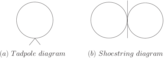
Figure 6: Contributions to the effective potential.

7.2.1 Finite-size corrections to the mass

To 1-loop approximation, the procedure follows along the same lines as in the previous subsection, starting from the expression for the one-loop contribution to the effective potential in unbounded space given by Eq. (243). The parameter $s$ in Eq. (243) counts the number of vertices on the loop. It follows that only the $s=1$ term contributes to the mass. It corresponds to the tadpole diagram in Fig. 6a. It is also clear that all $|\varphi_{0}|^{6}$-vertex and mixed $|\varphi_{0}|^{4}$- and $|\varphi_{0}|^{6}$ -vertex insertions on the 1-loop diagrams do not contribute when one computes the second derivative of similar expressions with respect to the classical field at zero value: only diagrams with two external legs would survive. This is impossible for a $|\varphi_{0}|^{6}$-vertex insertion at the 1-loop approximation. The first contribution from the $|\varphi_{0}|^{6}$ coupling must come from a higher-order term in the loop expansion. Two-loop diagrams with two external legs and only $|\varphi_{0}|^{4}$ vertices are of second order in its coupling constant, as well as all possible diagrams containing both type of vertices; all these diagrams are neglected. However, the 2-loop shoestring diagram, in Fig. 6b, with only one $|\varphi_{0}|^{6}$ vertex and two external legs is a first-order (in $\eta$) contribution to the effective potential and accordingly it is included in our approximation. In short, we consider the physical mass as defined to first-order in both coupling constants, by the contributions of radiative corrections from only two diagrams: the tadpole and the shoestring diagram.

The tadpole contribution to the effective potential is given by

$$U_{1}(\varphi_{0},L_{1},...,L_{d})=\frac{\lambda|\varphi_{0}|^{2}}{2\,\left(2\pi\right)^{D/2}}\left[2^{-D/2-1}m^{D-2}\Gamma\left(\frac{2-D}{2}\right)+F_{d}(D,m,\{L_{i}\})\right],$$ (294)

where

$$F_{d}(D,m,\{L_{i}\}) = \sum_{i=1}^{d}\sum_{n_{i}=1}^{\infty}\left(\frac{m}{L_{i}n_{i}}\right)^{D/2-1}K_{D/2-1}(mL_{i}n_{i})$$ (295)

$$+\,2\sum_{i<j=1}^{d}\sum_{n_{i},n_{j}=1}^{\infty}\left(\frac{m}{\sqrt{L_{i}^{2}n_{i}^{2}+L_{j}^{2}n_{j}^{2}}}\right)^{D/2-1}K_{D/2-1}\left(m\sqrt{L_{i}^{2}n_{i}^{2}+L_{j}^{2}n_{j}^{2}}\right)\,+\,\cdots$$

$$+\,2^{d-1}\sum_{n_{1},\ldots,n_{d}=1}^{\infty}\left(\frac{m}{\sqrt{L_{1}^{2}n_{1}^{2}+\cdots L_{d}^{2}n_{d}^{2}}}\right)^{D/2-1}K_{D/2-1}\left(m\sqrt{L_{1}^{2}n_{1}^{2}+\cdots L_{d}^{2}n_{d}^{2}}\right).$$

On the other hand, the 2-loop shoestring diagram contribution to the effective potential in unbounded space ($\{L_{i}=\infty\}$) is given by [12],

$$U_{2}(\phi_{0})=\frac{\eta|\varphi_{0}|^{2}}{16}\left[\int\frac{d^{D}q}{\left(2\pi\right)^{D}}\frac{1}{q^{2}+m^{2}}\right]^{2},$$ (296)

which is proportional to the square of the tadpole contribution. Then after compactification of $d$ dimensions with lengths $L_{i}$, $i=1,\ldots,d$ and integration over the non-compactified variables, $U_{2}$ becomes

$$U_{2}(\varphi_{0},L_{1},\ldots,L_{d})=\frac{\eta|\varphi_{0}|^{2}}{4\,\left(2\pi\right)^{D}\,}\left[2^{-1-D/2}m^{D-2}\Gamma\left(\frac{2-D}{2}\right)+\left[F_{d}(D,m,\{L_{i}\})\right]\right]^{2}.$$ (297)

In both Eqs. (294) and (297), there is a term proportional to $\Gamma\left(\frac{2-D}{2}\right)$ which as stated before, is divergent for even dimensions $D\geq 2$ and should be subtracted in order to obtain finite physical parameters. For odd $D$, the gamma function is finite, but we also subtract it (corresponding to a finite renormalization) for the sake of uniformity. After subtraction we get

$$U_{1}^{\mathrm{(Ren)}}(\varphi_{0},L_{1},\ldots,L_{d})=\frac{\lambda|\varphi_{0}|^{2}}{2\,\left(2\pi\right)^{D/2}}\,F_{d}(D,m,\{L_{i}\})$$ (298)

and

$$U_{2}^{\mathrm{(Ren)}}(\varphi_{0},L_{1},\ldots,L_{d})=\frac{\eta|\varphi_{0}|^{2}}{4\,(2\pi)^{D}}\,\left[F_{d}(D,m,\{L_{i}\})\right]^{2}.$$ (299)

Then the physical mass, to first-order in both coupling constants, is obtained using Eqs. (298) and (299) and also taking into account the contribution at the tree level; it satisfies a generalized Dyson-Schwinger equation depending on the lengths $L_{i}$ of the confining box,

$$m^{2}(T,\{L_{i}\})=m_{0}^{2}-\frac{\lambda}{\left(2\pi\right)^{D/2}}\,F_{d}(D,m,\{L_{i}\})+\frac{\eta}{2(2\pi)^{D}}\left[F_{d}(D,m,\{L_{i}\})\right]^{2},$$ (300)

where $F_{d}(D,m,\{L_{i}\})$ is given by Eq. (295).

7.2.2 Phase transition: films, wires and grains

A first-order transition occurs when all the three minima of the potential

$$U(\varphi_{0})=\frac{1}{2}m^{2}(T,\{L_{i}\})|\varphi_{0}|^{2}-\frac{\lambda}{4}|\varphi_{0}|^{4}+\frac{\eta}{6}|\varphi_{0}|^{6},$$ (301)

where $m(T,\{L_{i}\})$ is the physical mass defined above, are simultaneously on the line $U(\varphi_{0})=0$. This gives the condition

$$m^{2}(T,\{L_{i}\})=\frac{3\lambda^{2}}{16\eta}.$$ (302)

For $D=3$, the Bessel functions have the explicit form $K_{1/2}(z)=\sqrt{\pi}e^{-z}/\sqrt{2z}$; then, remembering that $m_{0}^{2}=\alpha(T/T_{0}-1)$, Eqs. (300) and (302) lead to the critical temperature for any specific situation.

Having developed the general case of a $d$-dimensional compactified subspace, it is now easy to obtain the specific formulas for particular values of $d$. If we choose $d=1$, the compactification of just one dimension, let us say, along the $x_{1}$-axis, we are considering that the system is confined between two planes, separated by a distance $L_{1}=L$. Physically, this corresponds to a film of thickness $L$ and the transition occurs at the $L$-dependent critical temperature

$$T_{c}^{\text{film}}(L) = T_{c}\left\{1-\left(1+\frac{3\lambda^{2}}{16\eta\alpha}\right)^{-1}\left[\frac{\lambda}{8\pi\alpha L}\ln\left(1-e^{-\sqrt{\frac{3\lambda^{2}}{16\eta}}L}\right)+\frac{\eta}{64\pi^{2}\alpha L^{2}}\left(\ln(1-e^{-\sqrt{\frac{3\lambda^{2}}{16\eta}}L})\right)^{2}\right]\right\},$$ (303)

where

$$T_{c}=T_{0}\left(1+\frac{3\lambda^{2}}{16\eta\alpha}\right)$$ (304)

is the bulk ($\{L_{i}\rightarrow\infty\}$) critical temperature for the first-order phase transition.

In the case $d=2$, the system is confined between two parallel planes a distance $L_{1}$ apart from one another normal to the $x_{1}$-axis and two other parallel planes, normal to the $x_{2}$-axis separated by a distance $L_{2}$. That is, the material is bounded within an infinite wire of rectangular cross section $L_{1}\times L_{2}$. To simplify matters, we take $L_{1}=L_{2}=L$ and the critical temperature is written in terms of $L$ as

$$T_{c}^{\text{wire}}(L)=T_{c}\left\{1-\left(1+\frac{3\lambda^{2}}{16\eta\alpha}\right)^{-1}\left[\frac{\lambda}{4\pi\alpha L}\,F_{2}(L)+\frac{\eta}{32\pi^{2}\alpha L^{2}}\,[F_{2}(L)]^{2}\right]\right\},$$ (305)

where

$$F_{2}(L)=2\ln\left(1-e^{-L\sqrt{\frac{3\lambda^{2}}{16\eta}}}\right)-2\sum_{n_{1},n_{2}=1}^{\infty}\frac{e^{-L\sqrt{\frac{3\lambda^{2}}{16\eta}}\sqrt{n_{1}^{2}+n_{2}^{2}}}}{\sqrt{n_{1}^{2}+n_{2}^{2}}}.$$ (306)

Finally, we may compactify all three dimensions, which leaves us with a system in the form of a cubic “grain” of some material. The dependence of the critical temperature on its linear dimension, $L_{1}=L_{2}=L_{3}=L$, is given by

$$T_{c}^{\text{grain}}(L)=T_{c}\left\{1-\left(1+\frac{3\lambda^{2}}{16\eta\alpha}\right)^{-1}\left[\frac{\lambda}{4\pi\alpha L}\,F_{3}(L)+\frac{\eta}{32\pi^{2}\alpha L^{2}}\,[F_{3}(L)]^{2}\right]\right\},$$ (307)

where

$$F_{3}(L)=3\ln\left(1-e^{-L\sqrt{\frac{3\lambda^{2}}{16\eta}}}\right)-2\sum_{j<i=1}^{3}\sum_{n_{i},n_{j}=1}^{\infty}\frac{e^{-L\sqrt{\frac{3\lambda^{2}}{16\eta}}\sqrt{n_{i}^{2}+n_{j}^{2}}}}{\sqrt{n_{i}^{2}+n_{j}^{2}}}-4\sum_{n_{1},\ldots,n_{3}=1}^{\infty}\frac{e^{-L\sqrt{\frac{3\lambda^{2}}{16\eta}}\sqrt{n_{1}^{2}+n_{2}^{2}+n_{3}^{2}}}}{\sqrt{n_{1}^{2}+n_{2}^{2}+n_{3}^{2}}}.$$ (308)

Let us observe that the general formalism employed in this section up to this point, involves extensions to several dimensions of the one-dimensional mode-sum regularization [77], which require, in particular, the definition of symmetrized multidimensional Epstein-Hurwitz functions with no analog in the one-dimensional case. It is this kind of mathematical framework that allows us to obtain general formulas, which may be particularized to films, wires and grains, thereby implying the peculiar forms of the critical temperature as a function of the linear dimension $L$, for these physically interesting cases.

It should be observed the very different form of Eqs. (303), (305) and (307) when compared with the corresponding ones for second-order transitions. In this last case the $L$-dependent transition temperature for films, wires and grains have the same functional dependence on the linear dimension, given by Eq. (276). We find that in all the cases (a film, a wire or a grain), there is a sharp contrast between the simple inverse linear behavior of $T_{c}(L)$ for second-order transitions (without considering corrections to the coupling constant) and the rather involved dependence on $L$ of the critical temperature for first-order transitions.

These two types of behavior demand to clarify the subject further; this can be done by comparing the theoretical curves with experimental data for superconducting materials. This has been considered for systems in the form of a film or of a wire in [80]. The interested reader will find there an explicitly comparison between the forms of the $T_{c}(L)$ curves for both first- and second-order transitions. Also in [80], the degree of agreement between theoretical expressions for the first-order critical temperature and some experimental results for a variety of transition-metal materials [292, 293, 294] is exhibited.

7.2.3 Effects of finite chemical potential

In what follows we study effects of the chemical potential on the size-dependent transition, particularly on the critical temperature. However, distinctly from the topics studied in the previous subsection, we take the squared mass $m_{0}^{2}$ as a fixed parameter of the model, not depending on temperature as in the GL model; now, temperature is introduced by means of methods of finite temperature field theory. To account for finite chemical potential effects, we consider the system at a temperature $\beta^{-1}$ and we compactify one of the spatial coordinates (say $x$) with a compactification length $L$; in this case, the Matsubara prescription, Eq. (183), has to be changed such that

$$k_{0}\equiv k_{\tau}\rightarrow\frac{2\pi n_{\tau}}{\beta}-i\mu.$$ (309)

Defining $a_{\tau}=1/(m\beta)^{2}$, $a_{x}=1/(mL)^{2}$, with $c^{2}=1/4\pi^{2}$, the one-loop contribution to the effective potential at finite chemical potential, can be written as

$$U_{1}(\varphi_{0},a_{\tau},a_{x})=\sum_{s=1}^{\infty}\frac{(-1)^{s+1}}{2s}\left[\lambda|\varphi_{0}|^{2}\right]^{s}\frac{m^{D-2s}}{\sqrt{a_{\tau}a_{x}}}\frac{1}{\left(4\pi^{2}\right)^{s}}\sum_{n_{\tau},n_{x}=-\infty}^{\infty}\int\,\frac{d^{D-2}\,k}{\left[\mathbf{k}^{2}+a_{\tau}\left(n_{\tau}-\frac{i\beta}{2\pi}\mu\right)^{2}+a_{x}n_{x}^{2}+c^{2}\right]^{s}}.$$ (310)

The integral in the above equation is calculated using the dimensional regularization formula in Eq. (186), so that the tadpole contribution to the effective potential becomes,

$$U_{1}(\varphi_{0},a_{\tau},a_{x})=\sum_{s=1}^{\infty}\frac{(-1)^{s+1}}{2s}\left[\lambda|\varphi_{0}|^{2}\right]^{s}\frac{m^{D-2s}}{\sqrt{a_{\tau}a_{x}}}\frac{\pi^{(D-2)/2}}{\left(4\pi^{2}\right)^{s}}\frac{\Gamma\left(s-\frac{D-2}{2}\right)}{\Gamma\left(s\right)}\sum_{n_{\tau},n_{x}=-\infty}^{\infty}\left[a_{\tau}\left(n_{\tau}-\frac{i\beta}{2\pi}\mu\right)^{2}+a_{x}n_{x}^{2}+c^{2}\right]^{(D-2)/2-s}.$$ (311)

The double sum in Eq. (311) may be recognized as the two-variable inhomogeneous Epstein-Hurwitz zeta function $Z_{2}^{c^{2}}(\nu;a_{\tau},a_{x};b_{\tau},b_{x})$, where $b_{\tau}=i\beta\mu/2\pi$, $b_{x}=0$ and $\nu=s-(D-2)/2$; this function possesses the analytical continuation given by Eq. (227).

After suppression of the singular term, using the symmetry property of Bessel functions, $K_{\nu}(z)=K_{-\nu}(z)$, and tanking the value of $\nu=s-(D-2)/2$ with $s=1$, the tadpole contribution to the effective potential is obtained as

$$U_{1}(\varphi_{0};\beta,L,\mu)=\frac{\lambda|\varphi_{0}|^{2}}{2\,\left(2\pi\right)^{D/2}}\,F(D,m,\beta,L),$$ (312)

where

$$F(D,m,\beta,L) = \sum_{n=1}^{\infty}\cosh\left(\beta\mu n\right)\left(\frac{m}{n\beta}\right)^{D/2-1}K_{D/2-1}\left(\beta mn\right)+\sum_{n=1}^{\infty}\left(\frac{m}{nL}\right)^{D/2-1}K_{D/2-1}\left(Lmn\right)$$ (313)

$$+\,2\sum_{n_{1},n_{2}=1}^{\infty}\cosh\left(\beta\mu n_{1}\right)\left(\frac{m}{\sqrt{\beta^{2}n_{1}^{2}+L^{2}n_{2}^{2}}}\right)^{D/2-1}K_{D/2-1}\left(m\sqrt{\beta^{2}n_{1}^{2}+L^{2}n_{2}^{2}}\right).$$

We now turn to the 2-loop shoestring diagram contribution to the effective potential, using again the Matsubara-modified Feynman rules prescription, Eq. (309), for the compactified dimensions. In unbounded space ($L\rightarrow\infty$), at zero temperature and chemical potential, it is given by Eq. (296). Then, at finite temperature and chemical potential, with one compactified spatial dimension, following steps analogous to those used to get $U_{1}$, we obtain

$$U_{2}(\varphi_{0};\beta,L,\mu)=\frac{\eta|\varphi_{0}|^{2}}{4\,(2\pi)^{D}}\left[F(D,m,\beta,L)\right]^{2},$$ (314)

where $F(D,m,\beta,L)$ is given by Eq. (313).

The mass is obtained from the normalization condition, Eq. (194),

$$m^{2}(\beta,L,\mu) = \left.\frac{\partial^{2}}{\partial\varphi_{0}^{2}}U(\varphi_{0};\beta,L,\mu)\right|_{\varphi_{0}=0}=\left.\frac{\partial^{2}}{\partial\varphi_{0}^{2}}\left(U_{\rm{tree}}+U_{1}(\varphi_{0};\beta,L,\mu)+U_{2}(\varphi_{0};\beta,L,\mu)\right)\right|_{\varphi_{0}=0}.$$

We now consider the three-dimensional Euclidean space ($D=3$), in which case the relevant Bessel functions are $K_{\pm 1/2}(z)=\sqrt{\pi}e^{-z}/\sqrt{2z}$. Then, after summing the geometric series, we get

$$m^{2}(\beta,L,\mu)=m_{0}^{2}+\frac{\lambda}{4\pi}\,F(\beta,L)+\frac{\eta}{16\pi^{2}}[F(\beta,L)]^{2},$$ (316)

where

$$F(\beta,L)=-\frac{1}{2\beta}\left[\ln\left(1-e^{-(m-\mu)\beta}\right)+\ln\left(1-e^{-(m+\mu)\beta}\right)\right]-\frac{1}{L}\ln\left(1-e^{-mL}\right)+2\sum_{n_{1},n_{2}=1}^{\infty}\cosh\left(\beta\mu n_{1}\right)\frac{e^{-m\sqrt{\beta^{2}n_{1}^{2}+L^{2}n_{2}^{2}}}}{\sqrt{\beta^{2}n_{1}^{2}+L^{2}n_{2}^{2}}}\,.$$ (317)

As in the previous subsection, a first-order transition occurs when all the three minima of the potential

$$U(\varphi_{0};\beta,L,\mu)=\frac{1}{2}m^{2}(\beta,L,\mu)|\varphi_{0}|^{2}-\frac{\lambda}{4}|\varphi_{0}|^{4}+\frac{\eta}{6}|\varphi_{0}|^{6},$$ (318)

are simultaneously on the line $U(\varphi_{0};\beta,L,\mu)=0$, which gives the condition ,

$$m^{2}(\beta,L,\mu)=\frac{3\lambda^{2}}{16\eta}.$$ (319)

It can be seen that for $0<\mu<m$ the double sum in Eq. (316) above for the mass converges. Then, using the condition (319), $m=\lambda\sqrt{3}/4\sqrt{\eta}$ in Eq. (316) we have a well-defined expression. It gives the critical temperature as a function of the compactification length $L$, of the chemical potential $\mu$, and of the fixed mass parameter $m_{0}$.

Figure 7: Critical temperature as a function of the inverse size , $x=1/L$, of the system in the horizontal axis. We take $\lambda=\eta=m_{0}=1$ in dimensionless units (mass scale $m_{0}$). From the lower to the upper curves, we have respectively, $\mu=0.40$ (full line), $\mu=0.35$ and $\mu=0.25$ (dot-dashed line). The symmetry-breaking regions are below each curve.

In order to perform a qualitative analysis of the phase structure of the model, we take for its parameters the values $\lambda=\eta=m_{0}=1$, in dimensionless units scaled by $m_{0}$. For these values, the condition in Eq. (319) implies that the dimensionless chemical potential is to be restricted to the range $0<\mu\lesssim 0.43$. In Fig. 7 we plot the critical temperature from Eq, (316) as a function of the inverse size of the system, $x=1/L$, for some values of the chemical potential. We find that for all values of $\mu$, the critical temperature decreases as the values of $x=1/L$ increase, in such a way that the symmetry breaking region under the curves is gradually diminished as the size of the system becomes smaller and smaller. Moreover, we find that there is a minimal allowed size for the system, for which this region disappears, a situation which is similar to the one encountered in the previous section. We interpret Fig. 7 as indicating that there is a minimal size of the system sustaining the transition; it is of the order (in the arbitrary units adopted here) of $L\sim 0.68$. This minimal size is independent of the chemical potential, although the detailed behavior of the critical temperature does depend on $\mu$. It is worth to remark that, we can reach this conclusion from an analysis of the critical equation, in an analogous way as it has been done in the previous section. Also, we find that for a fixed size of the system, the symmetry breaking region becomes smaller as the chemical potential increases. As an overall conclusion in this case, the results suggest that, also for first-order transitions, as the size of the system is diminished, finite-size effects start to appear for a given value of the compactification length, with the critical temperature decreasing as $L$ is further decreased, making the symmetry breaking region shrink. For the minimal size in Fig 7, the transition ceases to take place.

8 Phase transitions in four-fermions models on $\Gamma^{d}_{D}$

In this section, the quantum field theory on toroidal topology is considered for four-fermion interacting systems. The goal is to analyze the phase structure of such systems, focussing on applications in particle physics, although general results are useful in low energy physics.

In particle physics, the strong interaction, that have quarks and gluons as the basic constituents, presents a rather complicated structure that is hard to use at normal density and temperature of hadrons. It is usual then to depend on effective theories, that are attempts to assume that the gluon fields and the color degrees of freedom are integrated out, similarly to the Fermi treatment of the weak interaction. This provides the simplest effective models, which may be considered as four-fermion contact interaction among quarks. There are, at least, two schemes to achieve this: the Nambu-Jona-Lasino Model (NJL) [93, 94] and the Gross-Neveu (GN) model [95], where the latter is a sector of the former.

As effective theories for quantum chromodynamics (QCD), NJL and GN models have been enlightening approaches describing properties of hadronic matter. Those include asymptotical freedom in the high energy domain and investigations of the continuous and discrete chiral symmetry, which are associated with the confinement/deconfinement phase transition, both in the GN model [295, 296, 297, 298, 299, 300, 84, 87, 301, 302, 303, 304, 305, 306, 96, 307, 308, 309, 310, 311] and the NJL model [312, 313, 314, 315, 316, 317, 318, 319, 100, 99, 79, 101, 102, 103]. Rigorous QCD calculations, both at zero and finite temperature, have been worked out in order to describe such properties [320, 321], but mainly treating the asymptotically free domain at high energies or high temperatures, where perturbation theory is applicable. Actually, the intricate mathematical structure of QCD, practically prevents us from finding analytical results taking into account both confinement/deconfinement and asymptotic freedom. Four-fermion interaction models, as effective theory for QCD, are then practical tools mainly for the search of analytical results.

The four-fermion interaction model is also akin to the interaction among electrons in condensed matter physics. In particular, the GN model, is used to describe also properties of graphene, a honeycomb lattice with two Bravais triangular sublattices. The Hamiltonian of this structure is mapped in the (2+1) GN Hamiltonian, such that the $SU(4)$ chiral symmetry, arising from the arrangement of spins, can be broken into $SU(2)\times SU(2)$, where parity and time reversal invariance are preserved. This chiral symmetry breaking is the counterpart of a quantum phase transition from the semi-metallic phase to a gapped Mott insulator [322, 323, 324, 325, 87, 85, 326, 86]. Such a breaking of symmetry, that can be restored by raising the temperature, leads to a gap in the energy spectrum, that is of interest for electronic devices [327]. Similar four-fermion interaction is the fundamental aspect of the BCS theory for superconductivity. An important point to be emphasized here is that the susceptibility arising from the linear response theory has a divergence at a finite temperature, indicating the existence of a second-order phase transition between a disordered and a condensed phase [83]. As already mentioned in Section 6, spontaneous symmetry breaking is a common phenomenon in several domains of physics, and usually leads to underlying phase transitions [280]. Then considering applications in high energy physics, it may be anticipated in a study of four-fermion model that a phase transition appears, describing aspects of particle physics.

This is the case of the one-component massive tridimensional GN model at finite temperature [98]. In a $D$-dimensional Euclidian manifold, ${\mathbb{R}}^{D}$, we consider the Hamiltonian for the massive GN model,

$$H=\int d^{D}x\left\{\psi^{\dagger}(x)(i\gamma^{j}\partial_{j}-m_{0})\psi(x)+\frac{\lambda_{0}}{2}\left[\psi^{\dagger}(x)\psi(x)\right]^{2}\right\}$$ (320)

where $m_{0}$ and $\lambda_{0}$ are respectively the physical zero-temperature mass and coupling constant, $x\in{\mathbb{R}}^{D}$ and the $\gamma$-matrices are elements of the Clifford algebra (natural units $\hbar=c=k_{B}=1$ are used). This Hamiltonian is obtained by using conventions for Euclidian field theories in [328].

From Eq. (320), introducing the thermally corrected mass,

$$m(T)=m_{0}+\Sigma(T),$$ (321)

a generalization of the Ginzburg-Landau free energy density is

$${\mathcal{F}}=a+b(T)\phi^{2}(x)+c\,\phi^{4}(x),$$ (322)

where $b(T)=-m(T)$ and $c=\lambda_{0}/2$. The minus sign for the mass in Eq. (322) implies that, in the disordered phase we have $m(T)<0$ and for the ordered phase $m(T)>0$, consistently. The second order phase transition occurs at the temperature where $m(T)$ changes sign from negative to positive, characterizing a spontaneous symmetry breaking. In this formalism, the quantity $\phi(x)=\sqrt{\left\langle\psi^{\dagger}(x)\psi(x)\right\rangle}$, with $\left\langle\cdot\right\rangle$ meaning a thermal average, plays the role of the order parameter for the transition. The phase transition is obtained for a critical temperature, $T_{c}$, that is solution of the equation, $m(T)=0$. This gives rise to a function $T_{c}=T_{c}(m_{0};\lambda)$ [98].

A similar result is obtained from a non-perturbative analysis of the four-point function, by summing the chains of loop diagrams. This is the case of the aforementioned BCS approach [83]. The singularity of the leading contribution to the four-point function is related to the susceptibility, which diverges at a critical temperature. Then in general a singularity of the four-point function, of a four-fermion interacting system, indicates the existence of a phase transition.

It is worth mentioning that, although the GN model is not renormalizable for dimensions greater than $D=2$, the Euclidian model has been shown to exist and has been constructed for $D=3$ in the large-$N$ limit [329]. In any case, within the spirit of effective theories, perturbative renormalizability is not an absolute requirement for an effective theory to be a physically meaningful model [330, 331, 332, 333, 334]. This possibility has then been explored largely in literature, for both, GN and NJL models.

In the following, we apply to the GN and NJL models, the formalism of field theory on toroidal topology to investigate finite-size, density and magnetic field effects [335, 103]. Then the behavior of the four-point function of the massive $N$-component GN model on $\Gamma^{d}_{D}$ is discussed. Finally, we address the NJL model on this topology.

8.1 Phase transition in the massive Gross-Neveu model

8.1.1 Phase transition in one-component massive GN model

The one-component massive GN model in a $D$-dimensional Euclidian manifold, ${\mathbb{R}}^{D}$ is described by the Hamiltonian given in Eq. (320). Thermal and boundary corrections to $m_{0}$ and to $\lambda_{0}$ are defined by the temperature and boundary-dependent mass and coupling constant, $m(T,L)$ and $g(T,L)$ respectively, that assume the form

$$m(T,L)=m_{0}+\Sigma(T,L)$$ (323)

and

$$g(T,L)=\lambda_{0}[1+\lambda_{0}\Pi(T,L)]\;.$$ (324)

Then from Eq. (322), the generalized Ginzburg-Landau free energy density is

$${\mathcal{F}}=a-m(T,L)\phi^{2}(x)+g(T,L)\,\phi^{4}(x),$$ (325)

The minus sign for the mass in Eq. (325), as before, implies that, in the disordered phase we have $m(T,L)<0$ and for the ordered phase $m(T,L)>0$, consistently. A second order phase transition occurs in the region where $m(T,L)=0$, characterizing a spontaneous symmetry breaking.

At criticality, the leading contribution to the four-point function with zero-external momenta is given by the sum of all chains of one-loop diagrams, i.e.

$$\Gamma^{(4)}(\lambda_{0},T,L)=\frac{\lambda_{0}}{[1-\lambda_{0}\Pi(T,L)]}.$$ (326)

The first two terms of the expansion in powers of $\lambda_{0}$ of such a function are given in Eq. (324). The existence of a singularity of the four-point function in Eq. (326) indicates a phase transition; in other words, values of $T$ and $L$ solving the equation,

$$1-\lambda_{0}\Pi(T,L)=0\$$ (327)

assure a phase transition. The nature of the transition is obtained by a study of the free energy, Eq. (325). From an analysis of the infrared fixed point structure, the transition is of second order and that the critical temperature is determined by the condition $m(T,L)=0$. For a given value of $L$, this leads to a $L$-dependent critical temperature $T_{c}(L)$.

In order to evaluate the thermal and boundary dependent self-energy, $\Sigma(D;T,L)$, the generalized Matsubara formalism for fermion is used. This corresponds to take $c_{i}=1/2$ in Eq. (183), the modified Feynman rules. The Cartesian coordinates are specified by $\mathbf{r}=(x^{0},x^{1},\mathbf{z})$, where $\mathbf{z}$ is a $(D-2)$-dimensional vector. The conjugate momentum of $\mathbf{r}$ is denoted by $\mathbf{k}=(k_{0},k_{1},\mathbf{q})$.

At the one-loop level, the self-energy is given by $\Sigma(D;\beta,L;s)|_{s=1}$, where

$$\Sigma(D;\beta,L;s)=\lambda_{0}\frac{m_{0}}{\beta L}\sum_{n_{1},n_{2}=-\infty}^{\infty}\int\frac{d^{D-2}q}{(2\pi)^{D-2}}\frac{1}{(\mathbf{q}^{2}+\omega_{n_{1}}^{2}+\omega_{n_{2}}^{2}+m_{0}^{2})^{s}},$$ (328)

where $\omega_{n_{1}}$ and $\omega_{n_{2}}$ are Matsubara frequencies given by

$$\omega_{n_{1}}=\frac{2\pi(n_{1}+\frac{1}{2})}{\beta},\ \ \ \ \ \omega_{n_{2}}=\frac{2\pi(n_{2}+\frac{1}{2})}{L},$$

and $\beta=T^{-1}$. For using dimensional regularization procedure, the following dimensionless quantities are introduced: $a_{1}=(m_{0}\beta)^{-2}$ , $a_{2}=(m_{0}L)^{-2}$, $q_{j}=k_{j}/2\pi m_{0}$, for $j=3,...,D$, $\omega_{n_{i}}^{\prime}=\omega_{n_{i}}/2\pi m_{0}$, for $i=1,2$, and $c=1/2\pi$ . Then we get,

$$\Sigma(D;a_{1},a_{2};s)=\lambda_{0}m_{0}\sqrt{a_{1}a_{2}}\sum_{n_{1},n_{2}=-\infty}^{\infty}\int\frac{d^{D-2}q}{(2\pi)^{D-2}}\frac{1}{(\mathbf{q}^{2}+\omega_{n_{1}}^{\prime 2}+\omega_{n_{2}}^{\prime 2}+c^{2})^{s}}.$$

After dimensional regularization, we obtain

$$\Sigma(D;a_{1},a_{2};s)=\frac{m_{0}^{1-2\nu}\lambda_{0}\Gamma(\nu)}{(4\pi)^{(D-2)/2}\Gamma(s)}\,\sqrt{a_{1}a_{2}}\sum_{n_{1},n_{2}=-\infty}^{\infty}(\omega_{n_{1}}^{\prime 2}+\omega_{n_{2}}^{\prime 2}+c^{2})^{-\nu},$$ (329)

where $\nu=s-(D-2)/2$. This leads to

$$\Sigma(D;a_{1},a_{2};s)=\frac{m_{0}^{1-2\nu}\lambda_{0}\Gamma(\nu)4^{\nu}}{(4\pi)^{(D-2)/2}\Gamma(s)}\,\sqrt{a_{1}a_{2}}\left[Z_{2}^{4c^{2}}(\nu,a_{1},a_{2})-Z_{1}^{c^{2}}(\nu,a_{1})-\,Z_{1}^{c^{2}}(\nu,a_{2})+Z_{2}^{c^{2}}(\nu,4a_{1},4a_{2})\right],$$ (330)

where $Z_{d}^{b^{2}}(\nu,a_{1},a_{2})$ is the homogeneous Epstein-Hurwitz multi-variable zeta-function, given in Eq. (189), with analytical extension given in Eq. (190). For $s=1$ and $D=3$, such that $\nu=s-(D-2)/2=1/2$, performing the subtraction of divergent terms, following the procedure of Section 6, and using $K_{\pm 1/2}(z)=\sqrt{\pi}e^{-z}/\sqrt{2z}$ and $\sum_{n=1}^{\infty}e^{-\xi n}/n=-\ln(1-e^{-\xi})$, the self-energy reads

$$\Sigma(T,L)=m_{0}\,\frac{\lambda_{0}m_{0}}{2\pi}\,\mathcal{F}\left(\frac{m_{0}}{T},m_{0}L\right),$$ (331)

where

$$\mathcal{F}(x,y)=-\frac{\ln(1+e^{-x})}{x}-\frac{\ln(1+e^{-y})}{y}+\,2F(x,y)-4F(x,2y)-4F(2x,y)+8F(2x,2y),$$ (332)

with

$$F(x,y)=\sum_{n,l=1}^{\infty}\frac{\exp(-\sqrt{x^{2}n^{2}+y^{2}l^{2}})}{\sqrt{x^{2}n^{2}+y^{2}l^{2}}}.$$ (333)

Up to the one-loop level, the four-point function with null external momenta, which defines the $(\beta,L)$-dependent coupling constant, is

$$\Gamma_{D}^{(4)}(\beta,L;\lambda_{0})\simeq\lambda_{0}[1+\lambda_{0}\Pi(D,\beta,L)]\;,$$ (334)

where $\Pi(D,\beta,L)$ is the $(\beta,L)$-dependent one-loop polarization diagram given by

$$\Pi(D,\beta,L)=\frac{1}{\beta L}\sum_{n_{1},n_{2}=-\infty}^{\infty}\int\frac{d^{D-2}k}{(2\pi)^{D-2}}\frac{m_{0}^{2}-(\mathbf{k}^{2}+\omega_{n_{1}}^{2}+\omega_{n_{2}}^{2})}{(\mathbf{k}^{2}+\omega_{n_{1}}^{2}+\omega_{n_{2}}^{2}+m_{0}^{2})^{2}}.$$ (335)

Using the dimensionless quantities and subtracting the polar terms, as in the preceding section, the finite polarization reads

$$\Pi(T,L)=\frac{m_{0}}{2\pi}\,\mathcal{G}\left(\frac{m_{0}}{T},m_{0}L\right),$$ (336)

where the function $\mathcal{G}(x,y)$ is defined by

$$\mathcal{G}(x,y) = \frac{\ln(1+e^{-x})}{x}-\frac{1}{1+e^{x}}+\frac{\ln(1+e^{-y})}{y}-\,\frac{1}{1+e^{y}}$$ (337)

$$+2G(x,y)-4G(2x,y)-\,4G(x,2y)+8G(2x,2y),\hskip 28.45274pt$$

with

$$G(x,y)=\sum_{n,l=1}^{\infty}\exp\left(-\sqrt{x^{2}n^{2}+y^{2}l^{2}}\right)-F(x,y).$$ (338)

This provides us with the finite thermal and boundary-dependent coupling constant,

$$g(T,L;\lambda_{0})\equiv\Gamma_{3}^{(4)}(T,L,\lambda_{0})\simeq\lambda_{0}[1+\lambda_{0}\Pi(T,L))]\;.$$ (339)

The phase transition occurring in the GN model with a compactified spatial dimension is now discussed. Replacing in Eq. (332) $\lambda_{0}$ by $g(T,L;\lambda_{0})$ given in Eq. (339), we obtain a new self-energy, ${\mathcal{S}}(T,L;\lambda_{0})$, which incorporates the thermal and boundary corrections to the coupling constant. Then the $(T,L)$-dependent mass is

$$m(T,L) = m_{0}+{\mathcal{S}}(T,L;\lambda_{0})$$ (340)

$$= m_{0}\left\{1+\frac{\lambda_{0}m_{0}}{2\pi}\,\mathcal{F}\left(\frac{m_{0}}{T},m_{0}L\right)\left[1+\frac{\lambda_{0}m_{0}}{2\pi}\,\mathcal{G}\left(\frac{m_{0}}{T},m_{0}L\right)\right]\right\}$$

The phase transition condition , $m(T,L)=0,$ provides a critical surface defined by the critical temperature, the size of the system, $L$, and the the zero-temperature coupling constant in the the absence of boundaries, $\lambda_{0}$. This surface defines $L$-dependent values of the critical temperature, $T_{c}(L;\lambda_{0})$.

The dependence of $T_{c}$ on $\lambda_{0}$ is illustrated in Fig. 9, for some values of $L$. In Fig. 9, we present the behavior of the critical temperature as the length of the system diminishes, for some values of $\lambda_{0}$. From these plots, we find that there exists a minimal length below which the transition is suppressed. Moreover, we find that as the size of the system is diminished, the transition disappears [98]. The suppression of the transition below a minimal size is illustrated in Fig. 9 for several values of the fixed coupling constant.

Figure 8: Critical temperature in units of $m_{0}$, $t_{c}=T_{c}/m_{0}$, as a function ofthe free-space coupling constant (in units of $m_{0}^{-1}$), $\lambda=m_{0}\lambda_{0}/2\pi$, for some values of the compactification length (in units of $m_{0}^{-1}$), $l=m_{0}L$: $\infty$, 1.4 and 1.2 (full, dashed and dotted lines, respectively).

Figure 9: Critical temperature in units of $m_{0}$, $t_{c}=T_{c}/m_{0}$, as a function of the inverse of the compactification length (in units of $m_{0}$ ), $l^{-1}=1/m_{0}L$, for some values of $\lambda=m_{0}\lambda_{0}/2\pi$: 2.5, 4.0 and 10.0 (full, dashed and dotted lines, respectively).

These minimal sizes, $L_{\mathrm{min}}$, are characterized by the vanishing of the transition temperature and can be estimated. Take for instance the value $l_{\mathrm{min}}^{-1}\approx 0.826$ corresponding to $\lambda=5.0$ (the dashed curve in the figure). This gives $L_{\mathrm{min}}\approx 1.21\,m_{0}^{-1}$. Now, let us take for $m_{0}$, the mass of the Gross-Neveu fermion, to be the effective quark mass of the proton [336], $m_{0}\approx 330\,\mathrm{MeV}$. We get, using the conversion $1\,\mathrm{MeV}^{-1}=197\,\mathrm{fm}$, $L_{\mathrm{min}}\approx 0.72\,\mathrm{fm}$. This is of the order of magnitude of the estimated size of a meson, $L_{\mathrm{meson}}$, of $\sim 2/3$ of the size of a hadron, that is, $L_{\mathrm{meson}}\sim 0.92\,\mathrm{fm}$. Taking for instance the model defined by $\lambda=5.0$, it can be inferred from Fig. 9 that, for sizes of the system slightly larger than $L_{\mathrm{min}}\approx 0.72\,\mathrm{fm}$ (twice or more the minimum size), of order of magnitude of the estimated size of a meson, the transition temperature is $\sim 272\,\mathrm{MeV}$, which is compatible with the deconfining hadronic temperature. Similar results are obtained for other values of $\lambda$.

For completeness, an indication of a second-order transition is investigated from a renormalization group argument. In this case, the existence of an infrared stable fixed point at criticality can be shown from a study of the infrared behavior of the beta-function, $i.e.$ in the neighborhood of vanishing external momentum, $|p|\approx 0$. We consider the thermal boundary-dependent coupling constant at criticality $m=m(T_{c}(L))=0$, with an external small momentum $p$, given by

$$g(m=0;|p|\approx 0)=\frac{\lambda_{0}}{[1-\lambda_{0}\Pi(m=0;p)]}.$$ (341)

The one-loop polarization $\Pi(D,T,L,p)$ using a Feynman parameter $x$, and taking the mass parameter as the thermal boundary-dependent mass $m(T,L)$, which vanishes at criticality. We have,

$$\Pi(D,T,L,p)=\frac{1}{\beta L}\int_{0}^{1}dx\sum_{n_{1},n_{2}=-\infty}^{\infty}\int\frac{d^{D-2}k}{(2\pi)^{D-2}}\frac{m^{2}-(\mathbf{k}^{2}+\omega_{n_{1}}^{2}+\omega_{n_{2}}^{2})}{(\mathbf{k}^{2}+\omega_{n_{1}}^{2}+\omega_{n_{2}}^{2}+M_{x}^{2})^{2}},$$ (342)

where $M_{x}^{2}=M_{x}^{2}(p,T,L,x)=m^{2}(T,L)+p^{2}x(1-x)$ . For $|p|\approx 0$ and $D=3$, the polarization $\Pi(T,L,p)$ reads

$$\Pi(T,L,p)=\int_{0}^{1}\,dx\,\frac{M_{x}}{2\pi}\,\mathcal{G}\left(\frac{M_{x}}{T},M_{x}L\right).$$ (343)

At criticality, $m(T,L)=m(T_{c}(L))=0$, and for $|p|\sim 0$, keeping up to terms linear in $|p|$, from the above equation we get,

$$\Pi(T_{c},L,|p|\sim 0)\approx A(T_{c},L)|p|+B(T_{c},L)\,,$$ (344)

with $A(T_{c},L)=A=-\frac{1}{16}$ and

$$B(T_{c},L)=\left(\frac{T_{c}}{2\pi}+\frac{1}{2\pi L}\right)\ln 2-\mathcal{O}\left(\frac{1}{T_{c}},L\right)+\,2\mathcal{O}\left(\frac{1}{T_{c}},2L\right)+2\mathcal{O}\left(\frac{2}{T_{c}},L\right)-4\mathcal{O}\left(\frac{2}{T_{c}},2L\right),$$ (345)

where

$$\mathcal{O}(x,y)=\sum_{n,l=1}^{\infty}\frac{1}{\sqrt{x^{2}n^{2}+y^{2}l^{2}}}$$ (346)

and $\int_{0}^{1}\,dx\sqrt{x(1-x)}=\pi/8$ is used.

The coupling constant in Eq. (341) has dimension of $|p|^{-1}$. Taking $|p|$ as a running scale, we define a dimensionless coupling constant

$$g^{\prime}=|p|g=\frac{|p|\lambda_{0}}{1-\lambda_{0}[A(T_{c},L)|p|+B(T_{c},L)]}$$

and the beta-function,

$$\beta(g^{\prime})=|p|\frac{\partial\,g^{\prime}}{\partial|p|};$$ (347)

we find that the condition of a non-trivial infrared stable fixed point is fulfilled by the solution

$$g_{\star}^{\prime}=-\frac{1}{A}=16.$$ (348)

Then the infrared stable fixed point is independent of the length of the system and of the free-space coupling constant. We conclude that the phase transition, while it survives with decreasing $L$, is of second-order. We now discuss the $L$-dependence of the critical temperature.

8.1.2 Phase transition in the $N$-component massive GN model

We have pointed out that the four-point contact interaction of the GN model is similar to the delta-function interaction in the BCS theory of superconductivity. In the latter case, as in other systems of condensed matter, the susceptibility arising from the linear response theory has a divergence at a finite temperature, indicating the existence of a second-order phase transition between a disordered and an ordered i.e. a condensed phase [83]. As spontaneous symmetry breaking is the common feature underlying all phase transition phenomena [280], such a divergence would appear in other domains of physics [98]. Here, the existence of a phase transition in the massive $N$-component GN model on $\Gamma^{d}_{D}$ is investigated, by analyzing the four-point function in a non-perturbative way [335].

Particularly, the cases $D=2,3,4$ with all spatial dimensions compactified, initially at zero temperature are addressed, and then temperature effects are discussed by compactifying the imaginary time in a length $\beta=T^{-1}$, $T$ being the temperature. The behavior of the system as a function of its size and of the temperature are studied, focusing on the dependence of the large-$N$ coupling constant on the compactification length and temperature. Even at $T=0$, a singularity in the $4$-point function may appear driven by changes in the compactification length, suggesting the existence of a second-order phase transition in the system. This can be interpreted as a spatial confinement transition.

As in previous sections, we use concurrently dimensional and analytic regularizations and employ a subtraction scheme where the polar terms are suppressed. Results obtained with this procedure have similar structure for all values of $D$, which gives us confidence that they are meaningful for the $4$-dimensional space-time. In all cases, we obtain simultaneously an asymptotic freedom type of behavior for vanishingly small sizes of the system and spatial confinement, in the strong coupling regime, for low temperatures. As the temperature is increased, spatial confinement disappears, what is interpreted as a deconfining transition. The values of the confining lengths and the deconfining temperatures for $D=2,\;3\;{\rm{and}}\;4$ are calculated.

The massive GN model in a $D$-dimensional Euclidean space is described by the Wick-ordered Lagrangian density

$$\mathcal{L}=:\bar{\psi}(x)(i\,\gamma^{\mu}\partial_{\mu}+m)\psi(x):+\frac{u}{2}(:\bar{\psi}(x)\psi(x):)^{2},$$ (349)

where $m$ is the mass, $u$ is the coupling constant, $x$ is a point of $\mathbb{R}^{D}$ and the $\gamma$’s are the Dirac matrices. The quantity $\psi(x)$ represents a spin $\frac{1}{2}$ field having $N$ (flavor) components, $\psi^{a}(x)$, $a=1,2,...,N$, with summations over flavor and spin indices being understood in Eq. (349). The large-$N$ limit is considered, where $N\rightarrow\infty$ and $u\rightarrow 0$ in such way that $Nu=\lambda$ remains finite.

The large-$N$ (effective) coupling constant between the fermions on $\Gamma^{d}_{D}$ is defined in terms of the $4$-point function at zero external momenta. The $\{L_{i}\}$-dependent four-point function, at leading order in $\frac{1}{N}$, is given by the sum of chains of one-loop (bubble) diagrams, which can be formally expressed as

$$\Gamma_{Dd}^{(4)}(0;\{L_{i}\},u)=\;\frac{u}{1+Nu\Pi_{Dd}(\{L_{i}\})}.$$ (350)

The $\{L_{i}\}$-dependent one-loop Feynman diagram is given by

$$\Pi_{Dd}(\{L_{i}\})=\frac{1}{L_{1}\cdots L_{d}}\sum_{\{n_{i}\}=-\infty}^{\infty}\int\frac{d^{D-d}{\bf k}}{(2\pi)^{D-d}}\left[\frac{m^{2}-{\bf k}^{2}-\sum_{i=1}^{d}{\nu}_{i}^{2}}{\left({\bf k}^{2}+\sum_{i=1}^{d}{\nu}_{i}^{2}+m^{2}\right)^{2}}\right],$$ (351)

where the Matsubara frequencies $\nu_{i}$ are given by $\nu_{i}={2\pi(n_{i}+\frac{1}{2})}/{L_{i}}\;,\;\;i=1,2,...,d\,,$ such that $\{n_{i}\}=\{n_{1},\ldots,n_{d}\}$, with $n_{i}\in{\mathbb{Z}}$, and ${\bf k}$ is a $(D-d)$-dimensional vector in momentum space.

Introducing the dimensionless quantities $b_{i}=(mL_{i})^{-2}$ ($i=1,\dots,d$) and $q_{j}=k_{j}/2\pi m$ $(j=d+1,\dots,D)$, it is found

$$\Pi_{Dd}(\{b_{i}\})=\left.\Pi_{Dd}(s;\{b_{i}\})\right|_{s=2}=\frac{m^{D-2}}{4\pi^{2}}\sqrt{b_{1}\cdots b_{d}}\left.\left\{\frac{1}{2\pi^{2}}U_{Dd}(s;\{b_{i}\})-U_{Dd}(s-1;\{b_{i}\})\right\}\right|_{s=2},$$ (352)

where

$$U_{Dd}(\mu;\{b_{i}\})=\sum_{\{n_{i}\}=-\infty}^{\infty}\int\frac{d^{D-d}{\bf q}}{\left[{\bf q}^{2}+\sum_{j=1}^{d}b_{j}(n_{j}+\frac{1}{2})^{2}+(2\pi)^{-2}\right]^{\mu}}.$$ (353)

Using the dimensional regularization formula in Eq. (186) to perform the integral over ${\bf q}=(q_{d+1},\dots,q_{D})$ in Eq. (353), we obtain

$$U_{Dd}(\mu;\{b_{i}\})=\pi^{\frac{D-d}{2}}\,\frac{\Gamma(\mu-\frac{D-d}{2})}{\Gamma(\mu)}\sum_{\{n_{i}\}=-\infty}^{\infty}\left[\sum_{j=1}^{d}b_{j}\left(n_{j}+\frac{1}{2}\right)^{2}+(2\pi)^{-2}\right]^{\frac{D-d}{2}-\mu}.$$ (354)

The summations over half-integers in this expression can be transformed into sums over integers leading to

$$U_{Dd}(\mu;\{b_{i}\}) = \pi^{\frac{D-d}{2}}\,\frac{\Gamma(\mu-\frac{(D-d)}{2})}{\Gamma(\mu)}\,4^{\eta}$$ (355)

$$\times\left[Z_{d}^{h^{2}}(\eta,b_{1},\dots,b_{d})-\sum_{i=1}^{d}Z_{d}^{h^{2}}(\eta,\dots,4b_{i},\dots)\right.$$

$$\left.+\sum_{i<j=1}^{d}Z_{d}^{h^{2}}(\eta,\dots,4b_{i},\dots,4b_{j},\dots)-\cdots+(-1)^{d}\,Z_{d}^{h^{2}}(\eta,4b_{1},\dots,4b_{d})\right],$$

where $h^{2}=\pi^{-2}$, $\,\eta=\mu-\frac{D-d}{2}\,$ and

$$Z_{d}^{h^{2}}(\eta,\{a_{i}\})=\sum_{\{n_{i}\}=-\infty}^{\infty}\left[\sum_{j=1}^{d}a_{j}n_{j}^{2}+h^{2}\right]^{-\eta}$$ (356)

is the multiple ($d$-dimensional) Epstein-Hurwitz $zeta$-function.

The Epstein-Hurwitz $zeta$-function $Z_{d}^{h^{2}}(\eta,\{a_{i}\})$ is analytically extended to the whole complex $\eta$-plane [77, 281, 107]; we find

$$Z_{d}^{h^{2}}(\eta,\{a_{i}\}) = \frac{\pi^{\frac{d}{2}}}{\sqrt{a_{1}\cdots a_{d}}\,\Gamma(\eta)}\left[\frac{1}{h^{2(\eta-d)}}\Gamma\left(\eta-\frac{d}{2}\right)\right.$$ (357)

$$+\,\sum_{\theta=1}^{d}2^{\theta+1}\sum_{\{\sigma_{\theta}\}}\sum_{\{n_{\sigma_{\theta}}\}=1}^{\infty}\left(\frac{\pi}{h}\sqrt{\frac{n_{\sigma_{1}}^{2}}{a_{\sigma_{1}}}+\cdots+\frac{n_{\sigma_{\theta}}^{2}}{a_{\sigma_{\theta}}}}\right)^{\eta-\frac{d}{2}}\left.K_{\eta-\frac{d}{2}}\left(2\pi h\sqrt{\frac{n_{\sigma_{1}}^{2}}{a_{\sigma_{1}}}+\cdots+\frac{n_{\sigma_{\theta}}^{2}}{a_{\sigma_{\theta}}}}\right)\right],$$

where $\{\sigma_{\theta}\}$ represents the set of all combinations of the indices $\{1,2,\dots,d\}$ with $\theta$ elements and $K_{\alpha}(z)$ is the Bessel function of the third kind. Consequently, the function $U_{Dd}(\mu;\{b_{i}\})$ can also be analytically continued to the whole complex $\mu$-plane.

Taking $Z_{d}^{h^{2}}(\eta,\{a_{i}\})$ given in Eq. (357), grouping similar terms appearing in the parcels of Eq. (355) and using the identity

$$\sum_{j=1}^{N}\left(\frac{-1}{2}\right)^{j}\frac{N!}{j!(N-j)!}=\frac{1}{2^{N}}\,,$$ (358)

we obtain

$$U_{Dd}(\mu;\{b_{i}\})=\frac{2^{2\mu-D}\pi^{2\mu-\frac{D}{2}}}{\Gamma(\mu)}\frac{1}{\sqrt{b_{1}\cdots b_{d}}}\left[\Gamma\left(\mu-\frac{D}{2}\right)+2^{\frac{D}{2}}\,W_{Dd}(\mu;\{b_{i}\})\right]$$ (359)

with $W_{Dd}(\mu;\{b_{i}\})$ given by

$$W_{Dd}(\mu;\{b_{i}\})=2^{1-\mu}\sum_{j=1}^{d}2^{2j}\sum_{\{\rho_{j}\}}\sum_{\{c_{\rho_{k}}=1,4\}}\left(\prod_{k=1}^{j}\frac{(-1)^{c_{\rho_{k}}-1}}{\sqrt{c_{\rho_{k}}}}\right)\,F_{Dj}(\mu;c_{\rho_{1}}b_{\rho_{1}},\dots,c_{\rho_{j}}b_{\rho_{j}}),$$ (360)

where $\{\rho_{j}\}$ stands for the set of all combinations of the indices $\{1,2,\dots,d\}$ with $j$ elements and the functions $F_{Dj}(\mu;a_{1},\dots,a_{j})$, for $j=1,\dots,d$, are defined by

$$F_{Dj}(\mu;a_{1},\dots,a_{j})=\sum_{n_{1},\dots,n_{j}=1}^{\infty}\left(2\sqrt{\frac{n_{1}^{2}}{a_{1}}+\cdots+\frac{n_{j}^{2}}{a_{j}}}\right)^{\mu-\frac{D}{2}}K_{\mu-\frac{D}{2}}\left(2\sqrt{\frac{n_{1}^{2}}{a_{1}}+\cdots+\frac{n_{j}^{2}}{a_{j}}}\right).$$ (361)

Substituting Eq. (359) into Eq. (352) leads directly to an analytic extension of $\Pi_{Dd}(s;\{b_{i}\})$ for complex values of $s$, in the vicinity of $s=2$. We get,

$$\Pi_{Dd}(s;\{b_{i}\}) = \Pi_{Dd}^{{\rm polar}}(s)+2^{\frac{D}{2}}\left[2\,W_{Dd}(s;\{b_{i}\})-(s-1)\,W_{Dd}(s-1;\{b_{i}\})\right],$$ (362)

where

$$\Pi_{Dd}^{{\rm polar}}(s)=\frac{m^{D-2}\,\pi^{\frac{D}{2}}}{(2\pi)^{D-2s+4}\,\Gamma(s)}(s-1-D)\,\Gamma\left(s-1-\frac{D}{2}\right)$$ (363)

and the functions $W_{Dd}(\mu;\{b_{i}\})$ are given by Eq. (360).

It is important to notice that the first term in this expression for $\Pi_{Dd}(s;\{b_{i}\})$, $\Pi_{Dd}^{{\rm polar}}(s)$, does not depend on parameters $b_{i}$, that is, it is independent of the compactification lengths $L_{i}$ ($i=1,\dots,d$). At $s=2$, due to the poles of the $\Gamma$-function, such a term is divergent for even dimensions $D\geq 2$. Using again the minimal subtraction scheme, the finite one-loop diagram reads

$$\Pi_{Dd}(\{b_{i}\}) = \left[\Pi_{Dd}(s;\{b_{i}\})-\Pi_{Dd}^{\rm polar}(s)\right]_{s=2}$$ (364)

$$= \frac{m^{D-2}}{(2\pi)^{\frac{D}{2}}}\,\left[2\,W_{Dd}(2;\{b_{i}\})-W_{Dd}(1;\{b_{i}\})\right].$$

From now on, we shall deal only with finite quantities that are obtained following this subtraction prescription.

The large-$N$ ($\{b_{i}\}$-dependent) coupling constant, for $d$ ($\leq D$) compactified dimensions, is obtained by substituting $\Pi_{Dd}(\{b_{i}\})$ into Eq. (350) and taking the limit $N\rightarrow\infty$, $u\rightarrow 0$, with $Nu=\lambda$ fixed; we get

$$g_{Dd}(\{b_{i}\},\lambda)=\lim_{Nu=\lambda}\left[N\Gamma_{Dd}^{(4)}(0,\{b_{i}\},u)\right]=\frac{\lambda}{1+\lambda\,\Pi_{Dd}(\{b_{i}\})}.$$ (365)

It is clear that, while $g_{Dd}(\{b_{i}\},\lambda)$ depends on the value of the fixed coupling constant $\lambda$ in a direct way, its dependence on the compactifiation lengths is dictated by the behavior of $\Pi_{Dd}$ as $\{b_{i}\}$ is varied. The dependence of $g_{Dd}$ on $\{L_{i}\}$ and $\lambda$ is the main point to be discussed in the subsequent analysis.

For all the compactification lengths tending to infinity, i.e. $\{b_{i}\rightarrow 0\}$, thus reducing the problem to the free space at $T=0$, $\Pi_{Dd}\rightarrow 0$ and we obtain, consistently, that

$$\lim_{\{L_{i}\rightarrow\infty\}}g_{Dd}(\{b_{i}\},\lambda)=\lambda,$$ (366)

where $\lambda$ is the fixed coupling constant in free space at zero temperature. In the opposite limit, for any $b_{i}$ tending to $\infty$ (i.e. if any compactification length $L_{i}$ goes to $0$), the single bubble diagram $\Pi_{Dd}\rightarrow\infty$. This implies that the effective coupling constant $g_{Dd}$ vanishes, irrespective of the value of $\lambda$, suggesting that the system presents an asymptotic-freedom type of behavior for short distances and/or for high temperatures.

From the extreme limits considered above two situations may emerge, as one changes the compactification lengths from $0$ to $\infty$: either $\Pi_{Dd}$ varies from $\infty$ to $0$ through positive values, or $\Pi_{Dd}$ reaches $0$ before tending to $0$ through negative values. The latter case, which may actually happen, would lead to an interesting situation where a divergence of the effective coupling constant would appear at finite values of the lengths $L_{i}$. This possibility, and its consequences, will be investigated explicitly in the following.

For $D=2$ and $d=1$ (two-dimensional space-time with the spatial coordinate compactified), we put $b_{1}=(mL)^{-2}$ in Eqs. (360) and (361). In this case, we have

$$g_{21}(L,\lambda)=\frac{\lambda}{1+\lambda\,\Pi_{21}(L)},$$ (367)

where

$$\Pi_{21}(L)=2\,E_{1}(2mL)-E_{1}(mL),$$ (368)

with the function $E_{1}(x)$ being defined by

$$E_{1}(x)=\frac{1}{\pi}\sum_{n=1}^{\infty}\left\{-K_{0}(xn)+(xn)\,K_{1}(xn)\right\}.$$ (369)

The function $\Pi_{21}(L)$ is plotted as a function of $mL$ in Fig. 11. From this figure and the numerical treatment of Eq. (368), we infer that $\Pi_{21}(L)$ diverges ($\rightarrow+\infty$) when $L\rightarrow 0$ and tends to $0$, through negative values, as $L\rightarrow\infty$. Also, we find that $\Pi_{21}(L)$ vanishes for a specific value of $L$, which we denote by $L_{{\rm min}}^{(2)}$, being negative for all $L>L_{{\rm min}}^{(2)}$, and assumes a minimum (negative) value at a value of $L$ denoted by $L_{{\rm max}}^{(2)}$, for reasons that will be clarified later. Numerically, it is found that $L_{{\rm min}}^{(2)}\simeq 0.78\,m^{-1}\,$, $L_{{\rm max}}^{(2)}\simeq 1.68\,m^{-1}\,$ and $\Pi_{21}^{R\,{\rm min}}\simeq-0.0445$. This behavior of $\Pi_{21}$ as $L$ changes, particularly the fact that $\Pi_{21}(L)<0$ for $L>L_{{\rm min}}^{(2)}$, leads to remarkable properties of the large-$N$ coupling constant $g_{21}(L,\lambda)$.

The divergence of $\Pi_{21}(L)$ as $L\rightarrow 0$ ensures that, independently of the value of $\lambda$, $g_{21}(L,\lambda)$ approaches $0$ in this limit and, therefore, the system presents a kind of asymptotic-freedom behavior for short distances. On the other hand, since $\Pi_{21}(L)$ assumes negative values for $L>L_{{\rm min}}^{(2)}$, the denominator of Eq. (367) will vanish at a finite value of $L$ if $\lambda$ is sufficiently high. This means that, starting from a low value of $L$ (within the region of asymptotic freedom) and increasing the size of the system, $g_{21}$ will diverge at a finite value of $L$, $L_{c}^{(2)}(\lambda)$, if $\lambda$ is greater than the “critical value” $\lambda_{c}^{(2)}=(-\Pi_{21}^{R\,{\rm min}})^{-1}\simeq 22.47$. We interpret this result by stating that, in the strong-coupling regime ($\lambda\geq\lambda_{c}^{(2)}$) the system gets spatially confined in a segment of length $L_{c}^{(2)}(\lambda)$. The behavior of the $L$-dependent coupling constant as a function of $mL$ is illustrated in Fig. 11, for some values of the fixed coupling constant $\lambda$.

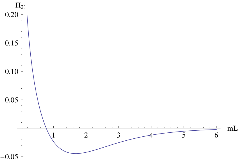
Figure 10: Plot of $\Pi_{21}(L)$ as a function of $mL$.          

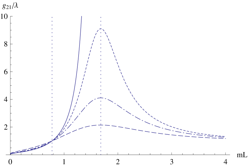
Figure 11: Plots of the relative effective coupling constant, $g_{21}(L,\lambda)/\lambda$, as a function of $mL$ for some values of $\lambda$: $20.0$ (dotted line), $17.0$ (dotted-dashed line), $12.0$ (dashed line) and $22.5$ (full line). The dotted vertical lines correspond to $L_{\rm min}^{(2)}\simeq 0.78\,m^{-1}$ and $L_{\rm max}^{(2)}\simeq 1.68\,m^{-1}$.

For $\lambda=\lambda_{c}^{(2)}$, by definition, the divergence of $g_{21}(L,\lambda)$ is reached as $L$ approaches the value that makes $\Pi_{21}$ minimal, which we have denoted by $L_{{\rm max}}^{(2)}$. In the other limit, since $g_{21}^{-1}(L,\lambda\rightarrow\infty)=\Pi_{21}(L)$, $L_{c}^{(2)}(\lambda)$ tends to $L_{{\rm min}}^{(2)}$, the zero of $\Pi_{21}(L)$, as $\lambda\rightarrow\infty$. In other words, the confining length $L_{c}^{(2)}(\lambda)$ decreases from the maximum value $L_{{\rm max}}^{(2)}$, when $\lambda=\lambda_{c}^{(2)}$, tending to the lower bound $L_{{\rm min}}^{(2)}$ in the limit $\lambda\rightarrow\infty$.

For the $3$-$D$ model at zero temperature with two compactified dimensions ($d=2$), denoting the compactification lengths associated with the two spatial coordinates $x_{1}$ and $x_{2}$ by $L_{1}$ and $L_{2}$ ($m^{-1}/\sqrt{b_{1}}$ and $m^{-1}/\sqrt{b_{2}}$, respectively); for simplicity we take $L_{1}=L_{2}=L$ and we obtain

$$\Pi_{32}(L_{1},L_{2})=\frac{m}{\pi}\left[\frac{1}{L}\log(1+e^{-L})-\frac{1}{1+e^{L}}+G_{2}(L,L)-4G_{2}(L,2L)+4G_{2}(2L,2L)\right],$$ (370)

where the function $G_{2}(x,y)$ is defined by

$$G_{2}(x,y) = \sum_{n,l=1}^{\infty}\exp\left(-\sqrt{x^{2}n^{2}+y^{2}l^{2}}\right)\left[1-\frac{1}{\sqrt{x^{2}n^{2}+y^{2}l^{2}}}\right].$$ (371)

The behavior of $\Pi_{32}(L)/m$ as a function of $mL$ is similar to that presented in Fig. 11 for $\Pi_{21}(L)$. We find, numerically, that $L_{{\rm min}}^{(3)}\simeq 1.30\,m^{-1}\,$ and $L_{{\rm max}}^{(3)}\simeq 2.10\,m^{-1}\,$, with $\Pi_{32}^{R\,{\rm min}}\simeq-0.00986\,m$. This behavior of $\Pi_{32}(L)$ has profound implications on the effective coupling constant. Thus for $D=3$ and $d=2$, Eq. (365) is rewritten as

$$g_{32}(L,\lambda)=\frac{\lambda}{1+\lambda\,\Pi_{32}(L)}.$$ (372)

We find that, for $\lambda\geq\lambda_{c}^{(3)}=(-\Pi_{32}^{R\,{\rm min}})^{-1}\simeq 101.42\,m^{-1}$, the denominator in Eq. (372) vanishes for a finite value of $L$, $L_{c}^{(3)}(\lambda)$, leading to a divergence in the effective coupling constant. The behavior of the effective coupling constant as a function of $L$, for increasing values of the fixed coupling constant $\lambda$, is illustrated showing the same pattern as that of Fig. 11 for the preceding case, with $L_{c}^{(3)}(\lambda)$ satisfying $L_{{\rm min}}^{(3)}<L_{c}^{(3)}(\lambda)\leq L_{{\rm max}}^{(3)}$.

For the $4$-$D$ GN model with all three spatial coordinates compactified, taking $L_{i}=L\,\,(i=1,2,3)$ measured in units of $m^{-1}$, we get

$$\Pi_{43}(L) = m^{2}\left[6H_{1}(2L)-3H_{1}(L)+6H_{2}(L,L)-24H_{2}(L,2L)+24H_{2}(2L,2L)\right.$$ (373)

$$-\left.4H_{3}(L,L,L)+24H_{3}(L,L,2L)-48H_{3}(L,2L,2L)+32H_{3}(2L,2L,2L)\right],$$

where the functions $H_{j}$, $j=1,2,3$, are defined by

$$H_{1}(x) = \frac{1}{2\pi^{2}}\sum_{n=1}^{\infty}\left[K_{0}(xn)-\frac{K_{1}(xn)}{(xn)}\right]\,,$$ (374)

$$H_{2}(x,y) = \frac{1}{2\pi^{2}}\sum_{n,l=1}^{\infty}\left[K_{0}\left(\sqrt{x^{2}n^{2}+y^{2}l^{2}}\right)-\frac{K_{1}(\sqrt{x^{2}n^{2}+y^{2}l^{2}})}{(\sqrt{x^{2}n^{2}+y^{2}l^{2}})}\right]\,,$$ (375)

$$H_{3}(x,y,z) = \frac{1}{2\pi^{2}}\sum_{n,l,r=1}^{\infty}\left[K_{0}\left(\sqrt{x^{2}n^{2}+y^{2}l^{2}+z^{2}r^{2}}\right)-\,\frac{K_{1}(\sqrt{x^{2}n^{2}+y^{2}l^{2}})}{(\sqrt{x^{2}n^{2}+y^{2}l^{2}+z^{2}r^{2}})}\right].$$ (376)

Similarly to the cases of $D=2$ and $D=3$, it is found numerically that $\Pi_{43}(L)$ vanishes for $L=L_{\rm min}^{(4)}\simeq 1.68\,m^{-1}$, being negative for $L>L_{\rm min}^{(4)}$, and assumes the minimum value, $\Pi_{43}^{R{\rm min}}\simeq-0.0022751\,m^{2}$, when $L=L_{\rm max}^{(4)}\simeq 2.37\,m^{-1}$. Therefore, the large-$N$ coupling constant,

$$g_{43}(L,\lambda)=\frac{\lambda}{1+\lambda\Pi_{43}(L)}\,,$$ (377)

diverges at a finite value of $L$, $L_{c}^{(4)}(\lambda)$, if $\lambda\geq\lambda_{c}^{(4)}=-(\Pi_{43}^{R{\rm min}})^{-1}\simeq 439.54\,m^{-2}$, meaning that the system gets confined in a cubic box of edge $L_{c}^{(4)}(\lambda)$ which is bounded in the interval between the values $L_{\rm min}^{(4)}$ and $L_{\rm max}^{(4)}$.

For $D=2,3,4$, with all spatial coordinates compactified with the same length, we find that the confining length lies in a finite interval, $L_{c}^{(D)}(\lambda)\in\left(L_{{\rm min}}^{(D)},L_{{\rm max}}^{(D)}\right],$ where the maximum value corresponds to $\lambda_{c}^{(D)}$, while $L_{{\rm min}}^{(D)}$ sets the bound as $\lambda\rightarrow\infty$. For a given value of $\lambda$ ($\geq\lambda_{c}^{(D)}$), the confining length $L_{c}^{(D)}(\lambda)$ is found numerically by determining the smallest root of the equation

$$g_{DD-1}^{-1}(L,\lambda)=\frac{1}{\lambda}\left[1+\lambda\Pi_{DD-1}(L)\right]=0.$$ (378)

That is, following the interpretation provided before, starting from small values of $L$, the first value at which $g_{DD-1}^{-1}$ vanishes does provide the confining length of the system, $L_{c}^{(D)}(\lambda)$.

Let us now consider the effect of raising the temperature on the effective coupling constant for the GN model, with all spatial dimensions compactified; this is implemented by the Matsubara procedure for the imaginagy-time. We generally expect that the dependence of $\Pi_{DD}$ and $g_{DD}$ on $\beta$ should follow similar patterns as that for the dependence on $L$. Like in the case where any compactification length $L_{i}$ tends to zero, we find that $\Pi_{DD}(L,\beta)\rightarrow\infty$ as $\beta\rightarrow 0$ ($T\rightarrow\infty$), implying that $g_{DD}\rightarrow 0$ independently of the value of the fixed coupling constant $\lambda$. This means that we have an asymptotic-freedom behavior for very high temperatures. For $\beta\rightarrow\infty$ ($T\rightarrow 0$), the behavior of $\Pi_{DD-1}(L)$ has been described earlier: for sufficiently high values of $\lambda$, the system is confined in a $(D-1)$-dimensional cube of edge $L_{c}^{(D)}$. Based on these observations, we expect that, starting from the compactified model at $T=0$ with $\lambda\geq\lambda_{c}^{(D)}$, raising the temperature will lead to the suppression of the divergence of $g_{DD}$ and the consequent spatial deconfinement of the system, at a specific value of the temperature, $T_{d}^{(D)}$.

Let us start with the $D=2$ GN model. To account for the effect of finite temperature, we take the second Euclidean coordinate (the imaginary time, $x_{2}$) compactified in a length $L_{2}=\beta=1/T$. In this case, replacing $b_{1}=L^{-2}$ and $b_{2}=\beta^{-2}$ ($L$ and $\beta$ measured in units of $m^{-1}$) into Eqs. (360), (361) and (364), the $L$ and $\beta$-dependent bubble diagram is written as

$$\Pi_{22}(L,\beta)=2\,E_{1}(2L)-E_{1}(L)+2\,E_{1}(2\beta)-E_{1}(\beta)+2\,E_{2}(L,\beta)-4\,E_{2}(2L,\beta)-4\,E_{2}(L,2\beta)+8\,E_{2}(2L,2\beta),$$ (379)

where the function $E_{1}(x)$ is given by Eq. (369) and the function $E_{2}(x,y)$ is defined by

$$E_{2}(x,y)=\frac{1}{\pi}\sum_{n,l=1}^{\infty}\left\{-K_{0}\left(\sqrt{x^{2}n^{2}+y^{2}l^{2}}\right)+\left(\sqrt{x^{2}n^{2}+y^{2}l^{2}}\right)\,K_{1}\left(\sqrt{x^{2}n^{2}+y^{2}l^{2}}\right)\right\}.\\$$

Notice that, in the limit $\beta\rightarrow\infty$, all $\beta$-dependent terms vanish and so $\Pi_{22}(L,\beta)$ reduces to the expression for zero temperature, $\Pi_{21}(L)$. For $\beta\rightarrow 0$, $\Pi_{22}(L,\beta)\rightarrow\infty$ and, independently of the value of $\lambda$, the system becomes asymptotically free. Therefore, raising the temperature leads to the suppression of the divergence of $g_{22}$ in the strong-coupling regime; i.e. for $\lambda\geq\lambda_{c}^{(2)}$, there exists a temperature, $T_{d}^{(2)}(\lambda)$, above which $g_{22}$ has no divergence and the system is spatially deconfined. The deconfining temperature $T_{d}^{(2)}(\lambda)$ is determined by finding the value of $T$ for which the minimum value of $g_{22}^{-1}(L,\beta,\lambda)$ changes from negative to positive.

The GN model in dimensions $D=3$ and $D=4$, with all spatial dimensions compactified and at finite temperature, can be analyzed along similar lines as for $D=2$. In all cases, the inverse of the effective coupling constant in given by

$$g_{DD}^{-1}(L,\beta;\lambda)=\frac{1}{\lambda}\left[1+\lambda\,\Pi_{DD}(L,\beta)\right].$$ (380)

The system is deconfined at a given temperature if the minimal value of $g_{DD}^{-1}(L,\beta;\lambda)$, with respect to changes in $L$, is positive. No matter how high the value of $\lambda$ is, the system becomes deconfined at a temperature $T_{d}^{(D)}(\lambda)\in\left[T_{\rm min}^{(D)},T_{\rm max}^{(D)}\right)$, with the limiting values corresponding to $\lambda_{c}^{(D)}$ and $\lambda\rightarrow\infty$, respectively. Notice that, $\,\min_{\{L\}}g_{DD}^{-1}(L,\beta;\lambda)=\left[1+\lambda\,M_{D}(\beta)\right]/\lambda$, where $M_{D}(\beta)=\min_{\{L\}}\Pi_{DD}(L,\beta)$. In the strong coupling regime, $\lambda\geq\lambda_{c}^{(D)}$, the deconfining temperature is determined by solving the equation $1+\lambda\,M_{D}(\beta)=0$; in this regime, this equation always has a solution, since $M_{D}(\beta\rightarrow\infty)=\Pi_{DD-1}^{R{\rm min}}=-[\lambda_{c}^{(D)}]^{-1}$, while $M_{D}(\beta)\rightarrow\infty$ as $\beta\rightarrow 0$. For $D=2$, we find $T_{\rm min}^{(2)}=[\beta_{\rm max}^{(2)}]^{-1}\simeq 0.65\,m$ and $T_{\rm max}^{(2)}\simeq 1.29\,m$; and, in the case of $D=3$, we have $T_{\rm min}^{(3)}\simeq 0.54m$ and $T_{\rm max}^{(3)}\simeq 0.88m$. For $D=4$, to avoid an anomalous behavior, we redefine the strong-coupling regime as $\lambda\geq\lambda_{d}^{(4)}\simeq 544.8\,m^{-2}$. The zero-temperature maximum confining length then becomes $L_{\rm max}^{(4)}\simeq 2.00\,m^{-1}$ and we find $T_{\rm min}^{(4)}\simeq 0.55\,m$ and $T_{\rm max}^{(4)}\simeq 0.70\,m$ [335]. The dependence of $T_{d}^{(D)}$ on $\lambda$ is depicted in Fig. 12, for $D=2$ and $D=4$; also, in this figure, the dependence of $L_{c}^{(D)}$ on $\lambda$ is presented.

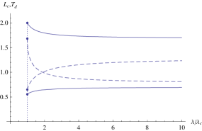
Figure 12: Deconfining temperature $T_{d}^{(D)}(\lambda)$ (in units of $m$), increasing curves, and confining length $L_{c}^{(D)}(\lambda)$ (in units of $m^{-1}$), decreasing curves, as a function of $\lambda/\lambda_{c}^{(D)}$, for $D=2$ (dashed lines) and $D=4$ (full lines).

The dependencies of $L_{c}^{(D)}$ and $T_{d}^{(D)}$ on the parameters $\lambda$ and $m$ are intrinsic results of the model. In all cases the confining length can be written as $L_{c}^{(D)}(\lambda)=f_{D}(\lambda)\,m^{-1}$, where the dimensionless functions $f_{D}(\lambda)$ are plotted in Fig. 12, for $D=2$ and $D=4$. The deconfining temperature is given by $T_{d}^{(D)}(\lambda)=h_{D}(\lambda)\,m$, where $h_{D}(\lambda)$ are dimensionless functions, also shown in Fig. 12. The functions $f_{D}(\lambda)$ and $h_{D}(\lambda)$ take on values in finite intervals ($\subset[0.5,2.1]$) and so it is found that extremely light fermions ($m\rightarrow 0$) are not confined at all, while extremely heavy ones ($m\rightarrow\infty$) would be strictly confined in a dot, no matter what the value of $\lambda$. Also, for all dimensions $D$, the product of $L_{c}^{(D)}\,T_{d}^{(D)}=f_{D}(\lambda)\,h_{D}(\lambda)$ is very close to the unit in the strong-coupling regime. However, to estimate values of $L_{c}^{(D)}$ and $T_{d}^{(D)}$ one needs to fix the parameter $m$, the mass of the fermions. Taking the GN model as an effective model for strong interaction, we choose $m\approx 350\,{\rm MeV}\simeq 1.75\,{\rm fm}^{-1}$, the constituent quark mass [337]. In this case one finds, for example, $0.96\,{\rm fm}<L_{c}^{(4)}<1.14\,{\rm fm}$ and $193\,{\rm MeV}<T_{d}^{(4)}<245\,{\rm MeV}$; these values compare amazingly well with the size of hadrons [338] and their estimated deconfining temperatures [160].

8.2 Finite size effects on the Nambu-Jona-Lasinio model

The Nambu-Jona-Lasinio (NJL) model [93, 94] provides more results useful for the investigation of dynamical symmetries when the system is under certain constraints, like finite temperature, space compactification, finite chemical potential, or gravitational field [339, 340, 341]. Boundary effects have been also considered for quark-meson models, in particular considering a toroidal topology [342, 343, 312, 313, 315, 317, 318, 319, 99, 100]. Here, we discuss finite-size effects on the dynamical symmetry breaking of the four-dimensional NJL model at finite temperature. This is carried out using zeta-function and dimensional regularization methods. This approach allows to determine analytically the size-dependence of the effective potential and the gap equation, and to study the phase structure of the compactified model. We also consider external magnetic-field effects on the system on the topology $\Gamma_{4}^{2}$, that is with one spatial coordinate compactified and at $T\neq 0$.

8.2.1 Effective potential and gap equation

Consider the massless version of the NJL model, described by the Lagrangian density,

$$\mathcal{L}=\bar{q}\,i\gamma{\partial}q+\frac{G}{2}\sum^{N^{2}-1}_{a=0}\left[\left(\bar{q}\alpha^{a}q\right)^{2}+\left(\bar{q}i\gamma_{5}\alpha^{a}q\right)^{2}\right],$$ (381)

where $q$ and $\bar{q}$ are the $N$-component spinors, the matrices $\alpha^{a}$ are the generators of the group $U(N)$, with $\alpha^{0}=\mathbf{I}/\sqrt{N}$, and $G$ is the coupling constant.

A bosonization procedure is performed assuming that only one auxiliary field, associated with the bilinear form $\sigma=\bar{q}\alpha^{0}q$, takes non-vanishing values and plays the role of a dynamical fermion mass, in the sense that the system is in the broken-chiral phase when it is non-zero. We consider the $D$-dimensional Euclidean space-time, particularizing to $D=4$ latter. We take $\sigma$ uniform so that the effective potential up to one-loop order, at leading order in $1/N$, is given by

$$\frac{1}{N}U_{eff}=\frac{\mathcal{A}_{eff}}{V}=\frac{\sigma^{2}}{2G}+U_{1}(\sigma),$$ (382)

where $\mathcal{A}_{eff}$ is the effective action, $V$ is the volume and

$$U_{1}(\sigma)=-h_{\mathbf{D}}\int\frac{d^{D}k}{(2\pi)^{D}}\ln{\left(\;\frac{k_{E}^{2}+\sigma^{2}}{\lambda^{2}}\right)},$$ (383)

where $h_{\mathbf{D}}$ is the dimension of the Dirac representation and $\lambda$ is a scale parameter.

To discuss finite-size effects on the phase structure, we take $d$ ($\leq D$) compactified dimensions and denote the Euclidian coordinate vectors by $x_{E}=(y,z)$, where $y=\left(x_{E}^{1},\dots,x_{E}^{d}\right)$ has components $y_{j}\in[0,L_{j}]$ while $z=\left(x_{E}^{d+1},\dots,x_{E}^{D}\right)$ refers to the non-compactified coordinates. Then, accordingly to the generalized Matsubara rules, the $k_{y}$-components of the the momentum $k_{E}$ take discrete values $k_{yj}\rightarrow 2\pi(n_{j}+c_{j})/L_{j}$, with $c_{j}=1/2$ for antiperiodic boundary conditions. For the system at finite temperature, with $d-1$ compactified spatial dimensions, we take $L_{1}\equiv\beta=1/T$.

Now, we rewrite Eq. (383) in terms of zeta-functions [107] as,

$$U_{1}(\sigma)=\frac{h_{\mathbf{D}}}{2V}\left[\zeta^{\,\prime}(0)+\ln{\lambda^{2}}\zeta(0)\right],$$ (384)

where $\zeta(s)$ is given by

$$\zeta(s)=V_{D-d}\sum_{n_{1},...,n_{d}=-\infty}^{+\infty}\int\frac{d^{D-d}k_{z}}{(2\pi)^{D-d}}\left[k_{z}^{2}+k_{y}^{2}+\sigma^{2}\right]^{-s},$$ (385)

where $k_{y}^{2}=\sum_{j=1}^{d}(4\pi^{2}/L_{j}^{2})\left(n_{j}+c_{j}\right)^{2}$, with $V_{D-d}$ being the $(D-d)$-dimensional volume. Performing the $k_{z}$-integration with dimensional regularization technique, we obtain

$$\zeta\left(s;\left\{a_{j}\right\},\left\{c_{j}\right\}\right)=\frac{V_{D-d}}{(4\pi)^{{D-d}/2}}\frac{\Gamma\left(s-\frac{{D-d}}{2}\right)}{\Gamma\left(s\right)}Z_{d}^{\sigma^{2}}\left(s-\frac{{D-d}}{2};\left\{a_{j}\right\},\left\{c_{j}\right\}\right),$$ (386)

where $Z_{d}^{\sigma^{2}}\left(\nu;\left\{a_{j}\right\},\left\{c_{j}\right\}\right)$ is the multivariable inhomogeneous Epstein-Hurwitz zeta function, defined by

$$Z_{d}^{\sigma^{2}}\left(\nu;\left\{a_{j}\right\},\left\{c_{j}\right\}\right)=\sum_{n_{1},...,n_{d}=-\infty}^{+\infty}\left[a_{1}(n_{1}+c_{1})^{2}+\cdots+a_{d}(n_{d}+c_{d})^{2}+\sigma^{2}\right]^{-\nu}.$$

The function $Z_{d}^{\sigma^{2}}$ is defined for $\rm{Re}\;\nu>d/2$, but it can be analytically continued to the whole complex $\nu$-plane. An analysis of the pole structure of the zeta-function implies that Eq. (384) can be written as [99, 107],

$$U_{1}\left(\sigma;\left\{a_{j}\right\},\left\{c_{j}\right\}\right)=\frac{h_{\mathbf{D}}}{2V_{d}(4\pi)^{(D-d)/2}}\Gamma\left(-\frac{D-d}{2}\right)Z_{d}^{\sigma^{2}}\left(-\frac{D-d}{2};\left\{a_{j}\right\},\left\{c_{j}\right\}\right),$$ (387)

for $D-d$ odd, or

$$U_{1}\left(\sigma;\left\{a_{j}\right\},\left\{c_{j}\right\}\right) = \frac{h_{\mathbf{D}}}{2V_{d}(4\pi)^{(D-d)/2}}\frac{(-1)^{\frac{D-d}{2}}}{((D-d)/{2})!}\left\{Z_{d}^{\sigma^{2}\,\prime}\left(-\frac{D-d}{2};\left\{a_{j}\right\},\left\{c_{j}\right\}\right)\right.$$ (388)

$$+\left.Z_{d}^{\sigma^{2}}\left(-\frac{D-d}{2};\left\{a_{j}\right\},\left\{c_{j}\right\}\right)\left[\ln{\lambda^{2}}-\gamma-\psi\left(\frac{D-d}{2}+1\right)\right]\right\},$$

for $D-d$ even, where $\gamma$ and $\psi(s)$ denote the Euler-Mascheroni constant and the digamma function, respectively.

To study the phase structure of the model, we analyze the gap equation, which is obtained by minimizing the effective potential with respect to $\sigma$,

$$\left.\frac{\partial}{\partial\sigma}U_{eff}\left(\sigma;\left\{a_{j}\right\},\left\{c_{j}\right\}\right)\right|_{\sigma=m}=0,$$ (389)

where $m$ is the dynamically generated fermion mass, that is the order parameter of the chiral phase transition.

Let us initially consider the model in $D=4$ without compactified coordinates ($d=0$) to set the free space parameters. In this case, the renormalized effective potential is given by

$$\frac{1}{N}U_{eff}\left(\sigma\right)=\frac{\sigma^{2}}{2G_{R}}+\frac{h_{\mathbf{D}}(D-1)}{(4\pi)^{D/2}}\Gamma\left(1-\frac{D}{2}\right)\lambda^{D-2}\sigma^{2}-\frac{h_{\mathbf{D}}}{D(4\pi)^{D/2}}\Gamma\left(1-\frac{D}{2}\right)\sigma^{D},$$ (390)

where the renormalized coupling constant $G_{R}$ is defined by

$$\frac{1}{G_{R}}=\frac{1}{G}-\frac{h_{\mathbf{D}}(D-1)}{(4\pi)^{D/2}}\Gamma\left(1-\frac{D}{2}\right)\lambda^{D-2}.$$ (391)

Note that Eq. (390) is valid for $2\leq D<4$, but it is singular for $D=4$ due to the pole of the gamma-function. Taking $h_{\mathbf{D}}=4$, in the vicinity of $D=4$, we have

$$\frac{1}{N}\frac{U_{eff}\left(\sigma\right)}{\lambda^{4}}=\frac{1}{2G_{R}}\frac{\sigma^{2}}{\lambda^{4}}-\frac{6\sigma^{2}}{(4\pi)^{2}\lambda^{2}}\left(\frac{1}{4-D}-\gamma+\ln{4\pi}+\frac{1}{3}\right)+\frac{\sigma^{4}}{(4\pi)^{2}\lambda^{4}}\left(\frac{1}{4-D}-\gamma+\ln{4\pi}+\frac{3}{2}-\ln{\frac{\sigma^{2}}{\lambda^{2}}}\right).$$ (392)

We can now compare this equation with the corresponding expression obtained using the cut-off regularization [344, 345],

$$\frac{1}{N}\frac{U_{eff}\left(\sigma\right)}{\lambda^{4}}=\frac{1}{2G}\frac{\sigma^{2}}{\lambda^{4}}-\frac{6\sigma^{2}}{(4\pi)^{2}\lambda^{2}}\left(\ln{\frac{\Lambda^{2}}{\lambda^{2}}}-\frac{2}{3}\right)+\frac{\sigma^{4}}{(4\pi)^{2}\lambda^{4}}\left(\ln{\frac{\Lambda^{2}}{\lambda^{2}}}+\frac{1}{2}-\ln{\frac{\sigma^{2}}{\lambda^{2}}}\right),$$ (393)

where the cut-off parameter $\Lambda$ must be larger than the scale $\lambda$. Thus, the zeta-function and cut-off methods are equivalent through the correspondence $1/(4-D)-\gamma+\ln{4\pi}+1\leftrightarrow\ln{\Lambda^{2}/\lambda^{2}}$. Hence, the non-trivial solution of the gap equation derived from Eq. (392) can be written as

$$\frac{1}{G_{c}}-\frac{1}{G_{0}}=-\frac{1}{m\lambda^{2}}\left.\frac{\partial}{\partial\sigma}U_{1}\left(\sigma\right)\right|_{\sigma=m}=\frac{4m^{2}}{(4\pi)^{2}\lambda^{2}}\ln{\frac{\Lambda^{2}}{m^{2}}},$$ (394)

where we have defined the dimensionless coupling constant $G_{c}=\lambda^{2}G_{R}$, and

$$\frac{1}{G_{0}}=\left.\frac{\partial}{\partial\sigma}U_{eff}\left(\sigma\right)\right|_{\sigma\rightarrow 0}=\frac{12}{(4\pi)^{2}}\left(\ln{\frac{\Lambda^{2}}{\lambda^{2}}}-\frac{2}{3}\right).$$ (395)

It is possible to identify the constant $G_{0}$ in Eq. (394) acting as a critical parameter; when $G_{c}>G_{0}$ we have a dynamically generated fermion mass. The value for $G_{0}$ can be chosen by fixing values for the mass scale $\lambda$ and the cut-off $\Lambda$ from phenomenological arguments.

To take into account finite-size and temperature effects, we have to analyze the modified gap equation,

$$\frac{1}{G_{c}}-\frac{1}{G_{0}}=-\frac{1}{\overline{m}\lambda^{2}}\left.\frac{\partial}{\partial\sigma}U_{1}\left(\sigma;\left\{a_{j}\right\},\left\{c_{j}\right\}\right)\right|_{\sigma=\overline{m}},$$ (396)

where $\overline{m}=\overline{m}(\{a_{j}\},\{c_{j}\})$ is the boundary-dependent fermion mass. Then, using Eqs. (387) and (388), the modified gap equation, Eq. (396), becomes

$$\frac{1}{G_{c}}=\frac{1}{G_{0}}+\frac{4}{\lambda^{2}V_{d}(4\pi)^{(D-d)/2}}\Gamma\left(1-\frac{D-d}{2}\right)Z_{d}^{\overline{m}^{2}}\left(-\frac{D-d}{2}+1;\left\{a_{j}\right\},\left\{c_{j}\right\}\right),$$ (397)

for $d=1,3$, while it has the form

$$\frac{1}{G_{c}}=\frac{1}{G_{0}}+\frac{4}{\lambda^{2}V_{2}4\pi}\left\{Z_{2}^{\overline{m}^{2}\,\prime}\left(0;\left\{a_{j}\right\},\left\{c_{j}\right\}\right)+Z_{2}^{\overline{m}^{2}}\left(0;\left\{a_{j}\right\},\left\{c_{j}\right\}\right)\left[\ln{\lambda^{2}}-\gamma-\psi\left(1\right)\right]\right\},$$ (398)

for $d=2$. Also, for $D=4$ we find

$$\frac{1}{G_{c}}=\frac{1}{G_{0}}-\frac{4}{\lambda^{2}V_{4}}\,{\rm FP}\left[Z_{4}^{\overline{m}^{2}}\left(1;\left\{a_{j}\right\},\left\{c_{j}\right\}\right)\right],$$ (399)

where ${\rm FP}[Z_{4}^{\overline{m}^{2}}]$ means the finite part of $Z_{4}^{\overline{m}^{2}}$. Thus, taking the fermion mass approaching to zero in Eqs. (397), (398) and (399), we obtain the critical values of the coupling constant $G_{c}$ with the corrections due to the presence of boundaries, for the cases $d=1,3$, $d=2$ and $d=4$, respectively. In this context, $\left.Z_{d}^{\overline{m}^{2}}\right|_{\overline{m}^{2}\rightarrow 0}$ reduces to a homogeneous generalized Epstein zeta-function $Z_{d}$.

The construction of the analytical continuation for $Z_{d}$ can be implemented using the generalized recurrence formula

$$Z_{d}\left(\nu;\left\{a_{j}\right\},\left\{c_{j}\right\}\right)=\frac{\Gamma\left(\nu-\frac{1}{2}\right)}{\Gamma(\nu)}\sqrt{\frac{\pi}{a_{d}}}\,Z_{d-1}\left(\nu-\frac{1}{2};\left\{a_{j\neq d}\right\},\left\{c_{j\neq d}\right\}\right)+\frac{4\pi^{s}}{\Gamma(\nu)}W_{d}\left(\nu-\frac{1}{2};\left\{a_{j}\right\},\left\{c_{j}\right\}\right),$$ (400)

where the symbol $\left\{a_{j\neq d}\right\}$ means that the parameter $a_{d}$ is excluded from the set $\left\{a_{j}\right\}$, and

$$W_{d}\left(\eta;\left\{a_{j}\right\},\left\{c_{j}\right\}\right)=\frac{1}{\sqrt{a_{d}}}\sum_{\{n_{j\neq d}\in\mathbb{Z}\}}\sum_{n_{d}=1}^{\infty}\cos{\left(2\pi n_{d}c_{d}\right)}\left(\frac{n_{d}}{\sqrt{a_{d}}X_{d-1}}\right)^{\eta}K_{\eta}\left(\frac{2\pi n_{d}}{\sqrt{a_{d}}}X_{d-1}\right)\;;$$ (401)

in the above equation $X_{d-1}=\sqrt{\sum_{k=1}^{d-1}a_{k}\left(n_{k}+c_{k}\right)^{2}}$.

8.2.2 Finite-size effects on the phase structure

We now examine the gap equation in the limit $\overline{m}\rightarrow 0$ in order to determine the $L_{j}$-dependent critical curves of the phase diagram. First, we study the compactification of spatial coordinates at zero temperature; for simplicity, we consider the same compactification length and antiperiodic boundary conditions for all coordinates, i.e. $L_{j}=L$ and $c_{j}=1/2$ for $j=1,\dots,d$. In this case, from Eqs. (397-401), we obtain

$$\frac{1}{G_{c}}=\frac{1}{G_{0}}-\frac{A_{d}}{(L\lambda)^{2}},$$ (402)

where $A_{1}=1/6$ and

$$A_{2} = A_{1}-\frac{4}{\pi}\sum_{n_{1}=-\infty}^{\infty}\sum_{n_{2}=1}^{\infty}(-1)^{n_{2}}\left(\frac{\left|n_{1}+\frac{1}{2}\right|}{n_{2}}\right)^{\frac{1}{2}}K_{-\frac{1}{2}}\left(2\pi n_{2}\left|n_{1}+\frac{1}{2}\right|\right)\approx 0.22,$$

$$A_{3} = A_{2}-\frac{4}{\pi}\sum_{n_{1},n_{2}=-\infty}^{\infty}\sum_{n_{3}=1}^{\infty}(-1)^{n_{3}}K_{0}\left(2\pi n_{3}\sqrt{\sum_{i=1}^{2}\left(n_{i}+\frac{1}{2}\right)^{2}}\right)\approx 0.26.$$

To illustrate the results above, in Fig. 14 we plot the critical coupling constant $G_{c}$, given by Eq. (402), as a function of $x=(L\lambda)^{-1}$; we also fix the value of $G_{0}\simeq 5.66$ by choosing $\Lambda\approx 1.25\,{\rm GeV}$ and $\lambda\approx 280\,{\rm MeV}$ [346]. For each of the three cases, the chiral breaking region lies above the corresponding curve. Since $G_{c}$ increases as $L$ decreases, we infer that diminishing the size of the system would require a stronger interaction to maintain it in the chiral breaking region.

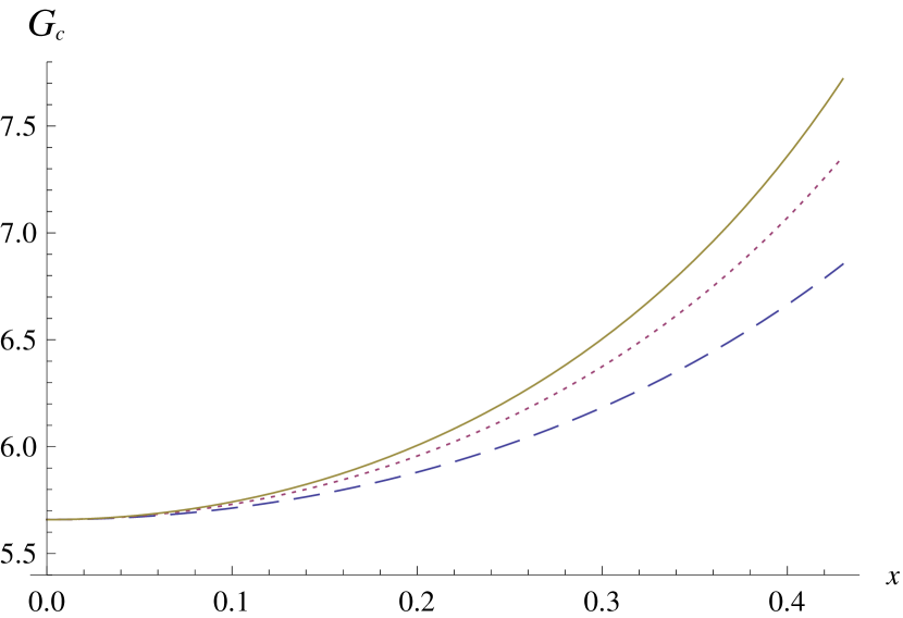
Figure 13: The critical coupling constant $G_{c}$, Eq. (402), as a function of $x=(L\lambda)^{-1}$. The dashed, dotted and solid lines correspond to the cases of $d=1,2,3$ compactified dimensions. We fixed $G_{0}\simeq 5.66$.

Figure 14: The phase diagram in the $(\chi,T)$-plane, where $\chi=(Lm)^{-1}$ and $T=(\beta m)^{-1}$. Dashed, dotted and solid lines represent $d=2,3,4$ compactified dimensions, respectively. For each case the non-trivial mass phase corresponds to the region below the corresponding line. The ratio between the parameters $\Lambda$ and $m$ is taken as $\Lambda/m=4.46$.

Consider now the system with compactified spatial dimensions at finite-temperature. We identify the first compactified coordinate with the Euclidian (imaginary) time, taking $L_{1}=\beta$. To study the $(L,T)$-dependent phase diagram, we have to analyze the critical equation obtained from Eqs. (394) and (396), that is

$$\frac{4m^{2}}{(4\pi)^{2}\lambda^{2}}\ln{\frac{\Lambda^{2}}{m^{2}}}+\frac{1}{\overline{m}\lambda^{2}}\left.\frac{\partial}{\partial\sigma}U_{1}\left(\sigma;\left\{a_{j}\right\},\left\{c_{j}\right\}\right)\right|_{\sigma=\overline{m}}=0,$$ (403)

where $a_{1}=4\pi^{2}/L_{1}^{2}\equiv 4\pi^{2}/\beta^{2}$ and, for simplicity, we take $a_{2}=\cdots=a_{d}=4\pi^{2}/L^{2}$. Proceeding as before, using again Eqs. (397-401) and taking the limit $\overline{m}\rightarrow 0$, we get:

$$\frac{4m^{2}}{(4\pi)^{2}}\ln{\frac{\Lambda^{2}}{m^{2}}}-\frac{A_{1}}{L^{2}}+\frac{4}{\pi L}\sum_{n_{1}=-\infty}^{\infty}\sum_{n_{2}=1}^{\infty}(-1)^{n_{2}}\left(\frac{\left|n_{1}+\frac{1}{2}\right|}{n_{2}\beta L}\right)^{\frac{1}{2}}K_{-\frac{1}{2}}\left(2\pi n_{2}\frac{\beta}{L}\left|n_{1}+\frac{1}{2}\right|\right)=0\;,\;\;\;{\rm{for}}\;d=2;$$ (404)

$$\frac{4m^{2}}{(4\pi)^{2}}\ln{\frac{\Lambda^{2}}{m^{2}}}-\frac{A_{2}}{L^{2}}+\frac{4}{\pi L^{2}}\sum_{n_{1},n_{2}=-\infty}^{\infty}\sum_{n_{3}=1}^{\infty}(-1)^{n_{3}}K_{0}\left(2\pi n_{3}\frac{\beta}{L}\sqrt{\left(n_{1}+\frac{1}{2}\right)^{2}+\left(n_{2}+\frac{1}{2}\right)^{2}}\right)=0\;,\;\;\;{\rm{for}}\;d=3;$$ (405)

$$\frac{4m^{2}}{(4\pi)^{2}}\ln{\frac{\Lambda^{2}}{m^{2}}}-\frac{A_{3}}{L^{2}}+\frac{4}{\pi L^{3}}\sum_{n_{1},n_{2},n_{3}=-\infty}^{\infty}\sum_{n_{4}=1}^{\infty}(-1)^{n_{4}}\left(\frac{n_{4}\beta L}{\sqrt{\sum_{i=1}^{3}\left(n_{j}+\frac{1}{2}\right)^{2}}}\right)^{\frac{1}{2}}K_{\frac{1}{2}}\left(2\pi n_{4}\frac{\beta}{L}\sqrt{\sum_{i=1}^{3}\left(n_{j}+\frac{1}{2}\right)^{2}}\right)=0\;,\;\;\;{\rm{for}}\;d=4.$$ (406)

The phase diagrams corresponding to Eqs. (404), (405) and (406) are plotted in Fig. 14, where $\chi=(Lm)^{-1}$ and $T=(\beta m)^{-1}$ are the inverse of the compactification length and the temperature, respectively, in units of $m$. Chiral breaking regions are below the lines while above them the system is in the chiral restoration phase. The critical temperature is maximum ($\approx 0.68m$) in free space ($\chi\rightarrow 0$), decreases as $\chi$ increases and vanishes at a critical value of the size of the system, $L_{c}$, corresponding to the minimal size of the system sustaining the chiral broken phase. For $D=4$, taking $m\approx 300\,{\rm MeV}$, one finds $T_{c}\simeq 204\,{\rm MeV}$ and $L_{c}\simeq 1.22\,{\rm fm}$.

The model can also be analyzed at finite density with or without compactified spatial dimensions. In both cases, it is found that nonzero values of the chemical potential can alter the order of the phase transition [79]. Next, we discuss properties of the finite-size fermion-fermion condensates under the influence of an external magnetic field.

8.2.3 Magnetic effects in the compactified system

An interesting aspect of the analysis, is to study changes in the phase transition induced by the finite size of the system in a magnetic background. These effects on four-fermion models, have been and still are the subject of intense investigation [312, 313, 314, 315, 316, 317, 318, 319, 100, 99, 79, 101, 102, 103]. The influence of an external magnetic field on the massless four-dimensional NJL model is considered. The Lagrangian density is

$${\cal L}=\bar{q}\;\left(i\gamma^{\mu}\partial_{\mu}-Q\gamma^{\mu}A_{\mu}\right)\;q+G\left[\left(\bar{q}q\right)^{2}+\left(\bar{q}i\gamma_{5}\overrightarrow{\tau}\,q\right)^{2}\right],$$ (407)

where $q$ and $\bar{q}$ are quark spinors carrying $N_{f}=2$ flavors and $N_{c}=3$ colors. The components of the vector $\overrightarrow{\tau}$ are the generators in the flavor space, $Q$ electric charge of the quark fields $(Q_{u}=2e/3,Q_{d}=-e/3)$, and $A^{\mu}$ is the four-potential associated to an external uniform magnetic field. We choose the gauge $A^{\mu}=(0,-x_{2}H,0,0)$, with $H$ being constant, which implies that the external magnetic field, ${\bf H}$, is parallel to the z axis. The Lagrangian density ${\cal L}$ is invariant under global chiral transformations, i.e. $q\rightarrow\exp{(i\theta\gamma_{5}\tau^{3}/2)}\;q$.

We introduce auxiliary fields $\sigma$ and $\pi$, defined by $2G\bar{q}q\equiv\sigma$ and $-2G\bar{q}i\gamma^{5}\tau^{3}\equiv\pi=\pi^{3}$ (we assume $\pi^{1}=\pi^{2}=0$). Then the Lagrangian density becomes,

$$\widetilde{{\cal L}}=\bar{q}\;\left(i\gamma^{\mu}\partial_{\mu}-Q\gamma^{\mu}A_{\mu}-\sigma-i\gamma^{5}\tau^{3}\pi\right)\;q-\frac{1}{4G}\left(\sigma^{2}+\pi^{2}\right),$$ (408)

which, after integration over the fermion fields $q$ and $\bar{q}$ generates the effective action,

$$\Gamma_{eff}(\sigma,\pi)=-\int d^{4}x\frac{1}{4G}\sigma^{2}-\frac{i}{2}\rm{Tr}\ln{\left(i\gamma^{\mu}\partial_{\mu}-Q\gamma^{\mu}A_{\mu}-\sigma-i\gamma^{5}\tau^{3}\pi\right)},$$ (409)

where $\rm{Tr}$ means the trace over the color, flavor, Dirac matrices and coordinate spaces.

We will study the pure chiral sector ($\pi=0$) and consider the mean-field approximation, which implies an uniform $\sigma$. Then the effective potential from Eq. (409) has the form,

$$U(\sigma) = \frac{\sigma^{2}}{4G}+\frac{i}{2V}\rm{Tr}\ln{\left(i\gamma^{\mu}\partial_{\mu}-Q\not{\!A}-\sigma\right)},$$ (410)

where $V$ is the four-dimensional volume. The fermion field, minimally coupled to the external magnetic field, obeys the Dirac equation,

$$\left(\gamma^{\mu}\partial_{\mu}-Q\gamma^{\mu}A_{\mu}-\sigma\right)q=0.$$ (411)

Applying again the Dirac operator, each component of $q$ satisfies the equation

$$\left[\left(i\partial+QA\right)^{2}-\frac{Q}{2}\sigma^{\mu\nu}F_{\mu\nu}-\sigma^{2}\right]q=0,$$ (412)

where $\sigma^{\mu\nu}=i[\gamma^{\mu},\gamma^{\nu}]/2$ and $F_{\mu\nu}=\partial_{\mu}A_{\nu}-\partial_{\nu}A_{\mu}$.

In the presence of the external magnetic field the natural basis is the set of the normalized eigenfunctions of the Landau basis. Then, the solutions of Eq. (412) are [278, 279, 347, 348],

$$q(x)=e^{i(p_{0}x_{0}-p_{1}x_{1}-p_{3}x_{3})}u(x_{2}),$$ (413)

where $u(x_{2})$ satisfies the equation,

$$\left[p_{2}^{2}+Q^{2}H^{2}\left(x_{2}-\frac{p_{1}}{QH}\right)^{2}\right]u(x_{2})=\left[p_{0}^{2}-p_{3}^{2}-\sigma^{2}\mp QH\right]u(x_{2}),$$ (414)

with

$$u_{n}(x_{2})=\frac{1}{\sqrt{2^{n}n!}}\left(\frac{QH}{\pi}\right)^{\frac{1}{4}}H_{n}\left(\sqrt{QH}\left[x_{2}-\frac{p_{1}}{QH}\right]\right);$$ (415)

here, $H_{n}$ are the Hermite polynomials and the energy spectrum provides the dispersion relation, $p_{0}^{2}=p_{3}^{2}+\sigma^{2}+(2n+1-s)QH$, with $n=0,1,2,...$, corresponding to the Landau levels, and $s=\pm 1$.

The introduction of the Landau basis implies a change in the momentum space integrations, as

$$\int\frac{d^{4}p}{(2\pi)^{4}}f(p)\rightarrow\frac{|Q|H}{2\pi}\sum_{s=\pm 1}\sum_{n=0}^{\infty}\int\frac{d^{2}p}{(2\pi)^{2}}f(p_{0},p_{3},n,s),$$

which leads to writing Eq. (410) in the form,

$$U(\sigma)=\frac{\sigma^{2}}{4G}+\frac{i}{2}{\rm{tr}}\frac{|Q|H}{2\pi}\sum_{s=\pm 1}\sum_{n=0}^{\infty}\int\frac{d^{2}p}{(2\pi)^{2}}\,\ln{\left[p_{0}^{2}-p_{3}^{2}-\sigma^{2}-(2n+1-s)QH\right]},$$ (416)

where $\rm{tr}$ means the trace over the color and flavor degrees of freedom.

Magnetic effects are accounted for by the introduction of the Landau basis, which “take out” two spatial dimensions. This corresponds, using Eq. (183), to writing the generalized Matsubara prescription in the form,

$$\int\frac{d^{2}p_{E}}{(2\pi)^{2}}f(p_{0},p_{3},n,s)\rightarrow\frac{1}{\beta L}\sum_{l,m=-\infty}^{\infty}f(\omega_{l},\omega_{m},n,s),$$ (417)

where we have performed the replacements,

$$p_{0} \rightarrow \omega_{l}=\frac{2\pi}{\beta}\left(l+\frac{1}{2}\right)-i\mu;\;l=0,\pm 1,\pm 2,\cdots,$$

$$p_{3} \rightarrow \omega_{m}=\frac{2\pi}{L}\left(m+\frac{1}{2}\right);\;\;\;m=0,\pm 1,\pm 2,...,$$

with $\mu$ being the chemical potential.

Using Eq. (417) in Eq. (416), after some manipulations, the effective potential with magnetic, finite-temperature and finite-size effects is given as,

$$U(\sigma)=\frac{\sigma^{2}}{4G}-\frac{N_{c}}{2}\sum_{f}\frac{|Q_{f}|H}{2\pi\beta L}\sum_{s=\pm 1}\sum_{n=0}^{\infty}\sum_{l,m=-\infty}^{\infty}\ln{\left[\omega_{l}^{2}+\omega_{m}^{2}+\sigma^{2}+(2n+1-s)|Q_{f}|H\right]},$$ (418)

where $f$ is the sum over the flavor indices.

The effective potential can be written in terms of Epstein-Hurwitz generalized zeta-functions, $Z^{c^{2}}_{2}(\eta)$, with $c^{2}=\sigma^{2}+(2n+1-s)|Q_{f}|H$, giving,

$$U(\sigma) = \frac{\sigma^{2}}{4G}+\sum_{f}\sum_{s=\pm 1}\frac{N_{c}|Q_{f}|H}{4\pi\beta L}Z^{c^{2}\,\prime}_{2}(0),$$ (419)

where the notation

$$Z^{c^{2}\,\prime}_{2}(0)=\left.\frac{\partial}{\partial\eta}Z^{c^{2}\,\prime}_{2}(\eta)\right|_{\eta=0}$$

is used. An analytical continuation of the generalized zeta-function $Z^{c^{2}}_{2}(\eta)$, to the whole complex $\eta$-plane, after use of recurrence formulas and some manipulations [99, 79, 107] leads to,

$$Z^{c^{2}}_{2}(\eta) = \frac{\beta L}{2\pi}\frac{\Gamma(\eta-1)}{\Gamma(\eta)}F_{1}(\eta-1)+\frac{\beta L}{\pi}\frac{1}{\Gamma(\eta)}F_{2}(\eta-1)+\frac{\beta}{\sqrt{\pi}}\frac{1}{\Gamma(\eta)}F_{3}\left(\eta-\frac{1}{2}\right).$$ (420)

The functions $F_{1}(\nu)$, $F_{2}(\nu)$ and $F_{3}(\nu)$ are respectively,

$$F_{1}(\nu) = (|Q_{f}|H)^{-\nu}\left[\zeta\left(\nu,\frac{\sigma^{2}}{|Q_{f}|H}\right)-\frac{1}{2}\left(\frac{\sigma^{2}}{|Q_{f}|H}\right)^{-\nu}\right],$$

$$F_{2}(\nu) = 2^{-\nu}\sum_{n=0}^{\infty}\sum_{m=1}^{\infty}\left(\frac{mL}{\sqrt{(2n+1-s)|Q_{f}|H+\sigma^{2}}}\right)^{\nu}(-1)^{m}K_{\nu}\left(mL\sqrt{(2n+1-s)|Q_{f}|H+\sigma^{2}}\right)$$

and

$$F_{3}(\nu) = 2^{1-\nu}\sum_{n=0}^{\infty}\sum_{m=-\infty}^{\infty}\sum_{l=1}^{\infty}\left(\frac{l\beta}{\sqrt{\frac{4\pi^{2}}{L^{2}}\left(m+\frac{1}{2}\right)^{2}+(2n+1-s)|Q_{f}|H+\sigma^{2}}}\right)^{\nu}(-1)^{l}$$

$$\times\,\cosh{(\mu\beta l)}K_{\nu}\left(l\beta\sqrt{\frac{4\pi^{2}}{L^{2}}\left(m+\frac{1}{2}\right)^{2}+(2n+1-s)|Q_{f}|H+\sigma^{2}}\right),$$

where $\zeta\left(\eta,a\right)$ is the inhomogeneous Riemann $zeta$-function. The function $Z^{c^{2}\,\prime}_{2}(\eta)$ may be analyzed using the pole structure of Eq. (420) for $\eta\rightarrow\epsilon$ ($\epsilon\ll 1$). We find that

$$\frac{d}{d\eta}\left[\frac{\Gamma(\eta-1)}{\Gamma(\eta)}F_{1}(\eta)\right]_{\eta\rightarrow\epsilon} \approx F_{1}(\epsilon-1)-F_{1}^{\prime}(\epsilon-1)-\epsilon F_{1}(\epsilon-1),$$

$$\frac{d}{d\eta}\left[\frac{1}{\Gamma(\eta)}F_{2}(\eta-1)\right]_{\eta\rightarrow\epsilon} \approx F_{2}(\epsilon-1),$$

$$\frac{d}{d\eta}\left[\frac{1}{\Gamma(\eta)}F_{3}\left(\eta-\frac{1}{2}\right)\right]_{\eta\rightarrow\epsilon} \approx F_{3}\left(\epsilon-\frac{1}{2}\right).$$

Then, for $\epsilon\rightarrow 0$, the effective potential is

$$U(\sigma) = \frac{\sigma^{2}}{4G}+U_{vac}-\sum_{f}\frac{N_{c}(|Q_{f}|H)^{2}}{2\pi^{2}}F_{4}\left(\frac{\sigma^{2}}{|Q_{f}|H}\right)+\sum_{f}\sum_{s=\pm 1}\frac{N_{c}|Q_{f}|H}{4\pi^{2}}\left[F_{2}\left(-1\right)+\frac{\pi^{\frac{1}{2}}}{L}F_{3}\left(-\frac{1}{2}\right)\right],$$ (421)

where

$$F_{4}(z)=\zeta^{\prime}\left(-1,z\right)-\frac{1}{2}\left(z^{2}-z\right)\ln{z}+\frac{z^{2}}{4}$$

and $U_{vac}$ is the vacuum contribution, given as

$$\frac{1}{N_{c}}U_{vac}=\frac{N_{f}}{8\pi^{2}}\left[\sigma^{4}\ln{\left(\frac{\Lambda+\sqrt{\Lambda^{2}+\sigma^{2}}}{\sigma}\right)}-\Lambda(2\Lambda^{2}+\sigma^{2})\sqrt{\Lambda^{2}+\sigma^{2}}\right],$$ (422)

$\Lambda$ being a cutoff parameter.

Then the gap equation is obtained from $\left.\partial U(\sigma)/\partial\sigma\right|_{\sigma=M}=0,$ where $M=M(T,\mu,L,H)$ is the $(T,\mu,L,H)$-dependent order parameter of the chiral symmetry breaking transition; equivalently $M$ plays the role of a dynamical fermion mass, such that when it has a non-vanishing value, the system is in the chiral broken phase. This generates one trivial solution, $M=0$, and other, non trivial ones, satisfying the equation,

$$\frac{1}{G}-\sum_{f}\frac{N_{c}(|Q_{f}|H)}{\pi^{2}}\;I\left(\frac{M^{2}}{|Q_{f}|H}\right)-\frac{1}{M}\left.\frac{\partial U_{vac}}{\partial\sigma}\right|_{\sigma=M}-\sum_{f}\sum_{s=\pm 1}\frac{N_{c}|Q_{f}|H}{\pi^{2}}\left[F_{2}\left(0\right)+\frac{\pi^{\frac{1}{2}}}{L}F_{3}\left(\frac{1}{2}\right)\right]=0,$$ (423)

where

$$I(z)=\ln{\Gamma(z)}-\frac{1}{2}\ln{2\pi}+z-\frac{1}{2}(2z-1)\ln{z},$$

and

$$\left(\frac{\partial U_{vac}}{\partial\sigma}\right)_{\sigma=M} = \frac{N_{c}N_{f}\,M}{\pi^{2}}\left[\Lambda\sqrt{\Lambda^{2}+M^{2}}-M^{2}\rm{ln}\left(\frac{\Lambda+\sqrt{\Lambda^{2}+M^{2}}}{M}\right)\right].$$ (424)

We recall that $M$ is the effective quark mass, $x=1/L$, $T=1/\beta$, $\omega=eH$ is the cyclotron frequency, $\mu$ is the chemical potential and $G$ is the coupling constant. It is interesting to introduce the critical coupling, $G_{c}$; in the absence of magnetic field, for vanishing temperature and chemical potential and in free space, it is given by $G_{c}=\pi^{2}/N_{c}N_{f}=\pi^{2}/6$. The region $G>G_{c}$ is the region with nontrivial mass.

In what follows all physical quantities are scaled by the ultraviolet cutoff parameter $\Lambda$, which has to be determined by fitting to experimental data; we take dimensionless quantities by performing the changes: $U/\Lambda^{4}\rightarrow U$; $M/\Lambda\rightarrow M$; $x/\Lambda\rightarrow x$; $T/\Lambda\rightarrow T$; $\omega/\Lambda^{2}\rightarrow\omega$; $\mu/\Lambda\rightarrow\mu$; and $1/G\Lambda^{2}\rightarrow 1/G$.

Figure 15: Plot of effective quark mass $M$ versus magnetic field from Eq. (423) at $T=0.001$, $\mu=0$, $G=\pi^{2}/6$. Solid, Dashed and dotted lines represent $x=0.01,0.5$ and $1$, respectively.

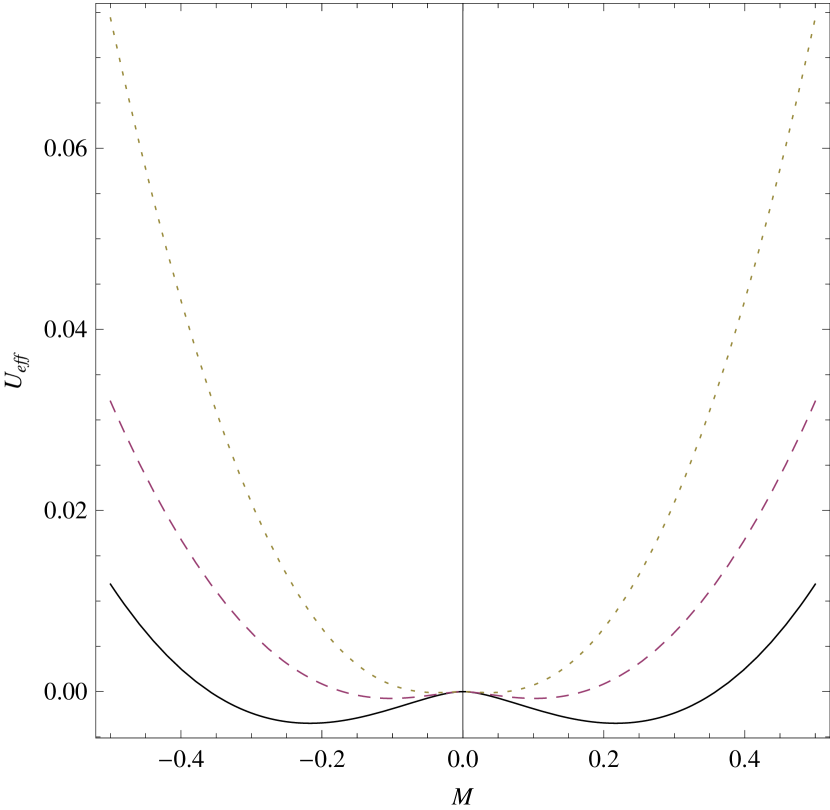
Figure 16: Plot of Effective potential in Eq. (421) at $T=0.001$, $\mu=0$, $G=\pi^{2}/12$ and $\omega=2$. Solid, Dashed and dotted lines represent values of the inverse size of the system, $x=0.01,0.5$ and $1.5$, respectively.

In Fig. 16 and Fig 16 we plot the effective quark mass $M$ versus magnetic field and the effective potential in Eq. (421) in terms of the inverse size of the system, $x$ respectively. From Eq. (423) at $\mu=0$, $i.e.$ in the absence of boundaries, at zero temperature, chemical potential and magnetic field. At fixed values of $T$, $\mu$ and $\omega$, there is a transition from the broken to the unbroken phase as the size of the system decreases; for fixed values of $T$, $\mu$ and $x$, there is a transition from the unbroken to the broken phase as the magnetic field increases. We find that the increasing of the magnetic field tends to drive the system to an ordered phase, an effect usually referred as magnetic catalysis. In addition, in Fig. 16, $M$ assumes a vanishing value at $\omega,\mu,T\approx 0$, an expected result for the coupling constant at the critical value. In the plot above of the effective potential, we see that the nature of phase transition is of second order. The first order transition is not observed, which could be a combined effect of insufficient magnetic field and finite-size effects.

Some points are worthy to be emphasized. For given values of the chemical potential and magnetic field, the appearance of the broken phase is inhibited as the size of the system decreases, $i.e.$, the decreasing of the size of the system makes it difficult to maintain long-range correlations and thus favors disorder. There exists a minimal size of the system below which the transition ceases to exist, in other words, the chiral-condensate phase cannot be sustained below this minimal size. Enhancement of the broken phase for a system with a finite size, occurs with increasing magnetic field, $i.e.$, the effective mass $M$ increases with $\omega$ at a fixed size of the system. Also, the dependence of $M$ on the intensity of the magnetic field is modified by the size of the system.

9 Compactified extra dimensions in low energy physics: Electrodynamics in $\Gamma_{5}^{1}$

Extra dimensions are explored; if they exist, they would manifest themselves in low energy physics. In particular, some consequences in quantum electrodynamics ${QED}$ would follow if our world were 5-dimensional. Some effects at the one-loop order are investigated under the assumption of a non-trivial vacuum with a non-vanishing magnetic flux along the extra compactified fifth dimension. Modifications of the vacuum polarization in extra dimension are considered. This is a procedure that has been employed in high energy physics to investigate, for instance, baryogenesis and electroweak transition, as a generalized version of the standard model [39, 13, 28, 29, 15, 30, 31, 32, 33, 34, 35, 36, 37, 38]. In particular, Panico and Serone consider the 5-D non-abelian gauge theory at finite temperature to study the electroweak phase transition. The compactified fifth dimension is then taken with a length $L$ having non-vanishing magnetic flux along it. This leads a first-order phase transition at temperature $T\sim 1/L$.

It is reasonable to consider that the presence of compactified extra dimensions may have effect not only in particle physics, but also in gravitation and atomic physics. This would imply that signatures of these extra dimensions might appear in phenomena governed by Newtonian gravitational forces, as it has been explored experimentally [50, 349, 350]. Also, low energy probes for the existence of extra dimensions are proposed [351], such as the effects on the anomalous magnetic moment of the muon, which has been associated with extra-dimensional excitations of the photon and of the W and Z bosons [41]. In addition, a value of $g_{\mu}\neq 2$ is not excluded by experiments [42]. Maybe this discrepancy can be explained as effects due to extra-dimensions [39, 40]. In particular, Roy and Bander [39] performed a calculation of $g_{\mu}-2$, assuming a 5-D space-time electroweak theory. They found a compactification length of the fifth dimension to be $\sim 10^{-16}$m.

Another interesting consequence of the possible existence of extra dimensions is that the electric charge may not be conserved exactly [45, 46, 47, 48]. In four-dimensional theories, a tiny deviation from electric charge conservation would lead to contradictions with low-energy tests of QED [45]. These deviations could be fixed by introducing millicharged particles [48] or by inclusion of high dimensions [45]. In this latter case, particles initially confined to $4$-dimensional space-time could, under some circumstances, migrate to extra dimensions. The idea is that if the particles are electrically charged, their migration from 4-dimension into extra dimensions would be considered as a non-conservation of electric charge. In atomic physics, measurements of the asymptotic quantum effects on excitations of Rydberg atoms have also been carried out [44, 43], and non-conservation of charge can be investigated in similar experiments.

In the following, some details of quantum electrodynamics on $\Gamma^{1}_{5}$ are reviewed as a possible theory for extra-dimension physics. Although an abelian theory is considered, the primary focus is on physical aspects that can be extended to non-abelian fields.

9.1 Quantum Electrodynamics in a compactified space

Consider the case of compactification of one spatial dimension in an ${\mathbb{R}}^{D}$ Euclidean spacetime, such that the topology of the resulting manifold is $\Gamma_{D}^{1}=({\mathbb{S}}^{1})\times{\mathbb{R}}^{D-1}$. For one compactified spatial dimension, from Eqs. (183), modified Feynman rules are

$$\int\frac{dk_{s}}{2\pi}\rightarrow\frac{1}{L}\sum_{n=-\infty}^{+\infty}\;;\;\;\;k_{s}\rightarrow\frac{2(n+c)\pi}{L}\;,$$ (425)

where $k_{s}$ stands for the momentum component corresponding to the compactified dimension, while $L$ is the size of the compactified spatial dimension. The quantity $c$ equals $0$ or $\frac{1}{2}$ for periodic or antiperiodic boundary condition, respectively .

One-loop effects for $QED_{3+1}$ are investigated with an extra compactified dimension, i.e. a 5-dimensional theory, in a non-trivial vacuum for the gauge field, defined by a non-vanishing component along the extra compactified dimension. The system is defined in terms of an Euclidean action, $S$, of the form,

$$S({\mathcal{A}};{\bar{\Psi}},\Psi)\;=\;S_{g}({\mathcal{A}})\,+\,S_{f}({\mathcal{A}};{\bar{\Psi}},\Psi)\;,$$ (426)

where $S_{g}$ and $S_{f}$ denote the $U(1)$ gauge field and fermion actions, respectively. The gauge action is assumed to be

$$S_{g}({\mathcal{A}})\;=\;\frac{1}{4}\,\int d^{5}x\,{\mathcal{F}}_{\alpha\beta}{\mathcal{F}}_{\alpha\beta}\;,$$ (427)

with ${\mathcal{F}}_{\alpha\beta}\equiv\partial_{\alpha}{\mathcal{A}}_{\beta}-\partial_{\beta}{\mathcal{A}}_{\alpha}$; we adopt the convention

$$\alpha,\beta,\dots\,=\,0,\,1,\,2,\,3,\,4\;,\;\;\;\mu,\nu,\dots\,=\,0,\,1,\,2,\,3\;,\;\;\;d^{5}x\;\equiv\;d^{3+1}x\,dx_{4}\,\,\,{\mathrm{and}}\,\,\,dx_{4}=ds,$$ (428)

with $x$ denoting the coordinates $x_{\mu}$ in ($3+1$) dimensions, unless the contrary is explicitly stated. The extra dimension is compactified with a radius $R$, so that $L=2\pi R\,.$ The Dirac action, $S_{f}$, is given by

$$S_{f}({\bar{\Psi}},\Psi;{\mathcal{A}})\;=\;\int d^{3+1}x\,ds\;{\bar{\Psi}}(x,s)\big{(}{\mathcal{D}}+m\big{)}\Psi(x,s)$$ (429)

where ${\mathcal{D}}$ is the $4+1$ dimensional Dirac operator, ${\mathcal{D}}=\gamma_{\alpha}D_{\alpha}$. The covariant derivative $D_{\alpha}\equiv\partial_{\alpha}+ig{\mathcal{A}}_{\alpha}$ includes a coupling constant $g$ with dimensions of $({mass})^{-\frac{1}{2}}$. For Dirac’s $\gamma$-matrices, we assume that $\gamma_{s}\equiv\gamma_{5}$, where the latter is the $\gamma_{5}$ matrix for the $3+1$ world.

The gauge field configuration ${\mathcal{A}}_{\alpha}(x,s)$ is decomposed into its zero ($A_{\alpha}$) and non-zero ($Q_{\alpha}$) mode components[28],

$${\mathcal{A}}_{\alpha}(x,s)\;=\;L^{-\frac{1}{2}}\,A_{\alpha}(x)\,+\,Q_{\alpha}(x,s)\;,$$ (430)

where the two terms are

$$A_{\alpha}(x)\;=\;L^{-\frac{1}{2}}\,\int_{0}^{L}ds\,{\mathcal{A}}_{\alpha}(x,s)\;,$$ (431)

and

$$Q_{\alpha}(x,s)\;=\;{\mathcal{A}}_{\alpha}(x,s)\,-\,L^{-\frac{1}{2}}\,A_{\alpha}(x).$$ (432)

The factor $L^{-\frac{1}{2}}$ is included in the zero mode term for this field to have the usual mass dimension in $3+1$ space-time. The Fourier expansion of the gauge field along the extra dimension is

$${\mathcal{A}}_{\alpha}(x,s)\;=\;L^{-\frac{1}{2}}\,\sum_{n=-\infty}^{\infty}\,e^{i\omega_{n}s}\,\widetilde{\mathcal{A}}_{\alpha}(x,n)\;,$$ (433)

with $\omega_{n}\equiv 2\pi n/L$, where

$$A_{\alpha}(x)\,=\,\widetilde{\mathcal{A}}_{\alpha}(x,0)\;\;,\;\;\;\;Q_{\alpha}(x,s)\,=\,L^{-\frac{1}{2}}\,\sum_{n\neq 0}\,e^{i\omega_{n}s}\,\widetilde{\mathcal{A}}_{\alpha}(x,n)\;.$$ (434)

The concept of dimensional reduction is defined by the limit of a compactified theory, where the size of the compactified dimension goes to zero. At this limit, with finite energy, zero is the only mode that survives along the compactified dimension. To dimensionally reduce a theory taking into account the Matsubara prescription, amounts to considering a compactified theory with small compactification lengths. Then only the zero mode component of the gauge field is kept. Therefore, we have

$$S_{g}({\mathcal{A}})\;\to\;S_{g}(A)\;=\;S_{g}(A_{\mu},\,A_{s})\;,$$ (435)

where

$$S_{g}(A_{\mu},A_{s})=\int d^{3+1}x\,\Big{[}\frac{1}{2}\partial_{\mu}A_{s}\partial_{\mu}A_{s}+\frac{1}{4}F_{\mu\nu}(A)F_{\mu\nu}(A)\Big{]},$$ (436)

with $F_{\mu\nu}(A)\equiv\partial_{\nu}A_{\nu}-\partial_{\nu}A_{\mu}$.

For the fermion action $S_{f}$, the reduction leads to

$$S_{f}({\mathcal{A}};{\bar{\Psi}},\Psi)\;\to\;S_{f}(A_{\mu},A_{s};{\bar{\Psi}},\Psi)\;.$$ (437)

Dimensional reduction of the fermion field is performed taking into account that, in the calculation of the effective gauge field action, its only contribution comes from the fermion loop. This loop may be represented as a series of $3+1$ dimensional loops, each one with a different mass (the different Matsubara frequencies). Contributions of heavier modes may be relatively suppressed, but the fact that there is an infinite number of them does not allow truncating that series.

After dimensional reduction, the fermion action becomes

$$S_{f}\;=\;\int d^{3+1}x\,\int_{0}^{L}ds\;{\bar{\Psi}}(x,s)\big{(}\not\!\!D+\gamma_{s}D_{s}+m\big{)}\Psi(x,s),$$ (438)

with

$$\not\!\!D\,=\,\gamma_{\mu}(\partial_{\mu}+ieA_{\mu})\;\;D_{s}\,=\,\partial_{s}+ieA_{s},$$ (439)

where we have introduced a new, dimensionless coupling constant $e\equiv gL^{-\frac{1}{2}}$, which plays the role of the electric charge in $3+1$ dimensions.

Considering the form of the gauge transformations in terms of the decomposition into zero and non-zero modes, $A_{\mu}$ transforms as a standard gauge field in $3+1$ dimensions [12],

$$\delta A_{\mu}(x)\,=\,\partial_{\mu}\alpha(x);$$ (440)

the extra dimensional component $A_{s}$ is a scalar in $3+1$-dimensions and is shifted by a constant, i.e.

$$\delta A_{s}(x)\,=\,\Omega\;.$$ (441)

The gauge field is coupled to the charged fermion field, whose transformation law under simultaneous action of the previous gauge transformation is

$$\Psi(x,s)\to e^{-ie[\alpha(x)+\Omega s]}\,\Psi(x,s)\,,\;\;\;\;\bar{\Psi}(x,s)\to e^{ie[\alpha(x)+\Omega s]}\,\bar{\Psi}(x,s)\;.$$ (442)

This implies that the constant $\Omega$ must be of the form $\Omega=2\pi k/Le$, where $k$ is an integer.

9.2 Effective action and parity conserving term

Let us first define a part of the effective action, $\Gamma(A)$, that depends only on the dimensionally reduced gauge field,

$$\Gamma(A)\;\equiv\;\Gamma(A;{\bar{\Psi}},\Psi)\Big{|}_{{\bar{\Psi}}=\Psi=0}\;,$$ (443)

where $\Gamma(A;{\bar{\Psi}},\Psi)$ is the full effective action. From the functional $\Gamma(A)$, one-particle-irreducible functions are derived, having as external lines only components of the gauge field, $A_{\mu}$, $A_{s}$. The components $A_{\mu}$ have a clear interpretation in $(3+1)$-dimensional space-time. However, $A_{s}$, that has no direct meaning, is assumed to have a constant value, which is determined by an external condition to the model. The fermion one-loop gives the only non-trivial contribution to $\Gamma(A)$, i.e.

$$\Gamma(A)\;=\;\Gamma^{(0)}(A)\,+\,\Gamma^{(1)}(A)\;+\;\cdots,$$ (444)

where $\Gamma^{(0)}(A)=S_{g}(A)$ and

$$e^{-\Gamma^{(1)}(A)}\;=\;\int{\mathcal{D}}\Psi{\mathcal{D}}{\bar{\Psi}}e^{-S_{f}(A;{\bar{\Psi}},\Psi)}\;.$$ (445)

The focus here will be on the effective action for the gauge field components $A_{\mu}$, that have a physical meaning for the $3+1$-dimensional theory. Following Panico and Serone [28], $A_{s}$ is assumed to be such that it yields a non-vanishing flux,

$$e\int_{0}^{L}dsA_{s}\;=\;\theta,$$ (446)

where $\theta$ is a constant. A simple solution is to take $A_{s}$ as a constant given by

$$A_{s}\;=\;\frac{\theta}{eL}\;,$$ (447)

which fixes the gauge. Since the gauge transformations shift $A_{s}$ by an integer multiple of $2\pi/eL$, the value of $\theta$ may be fixed in the domain $0\leq\theta<2\pi$. This will be assumed in what follows. Such a gauge field configuration may be interpreted as a topological effect, in the sense that it corresponds locally, although not globally, to a pure gauge field configuration [40].

Performing a Fourier expansion of the fermion field along the $s$ coordinate,

$$\Psi(x,s)=L^{-\frac{1}{2}}\,\sum_{n=-\infty}^{\infty}e^{i\omega_{n}s}\psi_{n}(x)\,,\;\;\;{\bar{\Psi}}(x,s)=L^{-\frac{1}{2}}\,\sum_{n=-\infty}^{\infty}e^{-i\omega_{n}s}{\bar{\psi}}_{n}(x)\;,$$ (448)

and inserting into the functional expression for $\Gamma^{(1)}(A)$, we get,

$$S_{f}\;=\;\sum_{n=-\infty}^{n=+\infty}\int d^{3+1}x\,\bar{\psi}_{n}(x)\left(\not\!\!D+i\gamma_{s}\left(\omega_{n}+\frac{\theta}{L}\right)+m\right)\psi_{n}(x)\;.$$ (449)

Using the same expansion, the fermion measure factorizes in the form,

$$\mathcal{D}\Psi\mathcal{D}\bar{\Psi}\;=\;\prod_{n=-\infty}^{n=+\infty}\mathcal{D}\psi_{n}(x)\mathcal{D}\bar{\psi}_{n}(x);$$ (450)

then the Euclidean action corresponding to each mode $n$ may be written as

$$\int d^{3+1}x\,\bar{\psi}_{n}(x)\left(\not\!\!D+i\gamma_{s}\left(\omega_{n}+\frac{\theta}{L}\right)+m\right)\psi_{n}(x)=\;\int d^{3+1}x\,\,\bar{\psi}_{n}(x)(\not\!\!D+M_{n}\,e^{-i\varphi_{n}\gamma_{5}})\psi_{n}(x),$$ (451)

where

$$M_{n}\equiv\sqrt{m^{2}+(\omega_{n}+\theta/L)^{2}}\;,\;\;\;\varphi_{n}={\rm arctan}(\frac{\omega_{n}+\theta/L}{m})\;.$$ (452)

The $\gamma_{5}$ term implies that parity symmetry can be broken. Performing a change in the fermion variables such that the explicit dependence on $\gamma_{5}$ is suppressed, then we have

$$\psi_{n}(x)\to e^{-i\gamma_{5}\varphi_{n}/2}\psi_{n}(x)\,,\,\,\,\,\bar{\psi}_{n}(x)\to\bar{\psi}_{n}(x)e^{i\gamma_{5}\varphi_{n}/2}.$$ (453)

Then the mode labeled by $n$ has the action,

$$\int d^{3+1}x\,\,\bar{\psi}_{n}(x)(\not\!\!D+M_{n}\,e^{-i\varphi_{n}\gamma_{5}})\psi_{n}(x)\;.$$ (454)

Now $\Gamma^{(1)}$ may be written as follows,

$$e^{-\Gamma^{(1)}(A)}\;=\;\prod_{n=-\infty}^{+\infty}\Big{[}{\mathcal{J}}_{n}\;e^{-\Gamma^{(1)}_{3+1}(A,M_{n})}\Big{]}\;,$$ (455)

where we have the Jacobian,

$${\mathcal{J}}_{n}\;=\;\exp\big{(}\frac{ie^{2}}{16\pi^{2}}\,\varphi_{n}\int d^{3+1}x{\tilde{F}}_{\mu\nu}F_{\mu\nu}\big{)}\;,$$ (456)

with ${\tilde{F}}_{\mu\nu}=\frac{1}{2}\epsilon_{\mu\nu\rho\lambda}F_{\rho\lambda}$. The quantity $\Gamma^{(1)}_{3+1}(A,M_{n})$ is the one-loop fermion contribution to the effective action, for a fermion whose mass is $M_{n}$, in $3+1$ dimensions. It may be expressed as a fermion determinant,

$$e^{-\Gamma^{(1)}_{3+1}(A,M_{n})}\;=\;\det(\not\!\!D+M_{n})\;.$$ (457)

A general expression for the one loop effective action is

$$\Gamma^{(1)}(A)\;=\;\Gamma^{(1)}_{e}(A)\,+\,\Gamma^{(1)}_{o}(A),$$ (458)

where

$$\Gamma^{(1)}_{e}(A)\;=\;\sum_{n=-\infty}^{\infty}\Gamma^{(1)}_{3+1}(A,M_{n}),$$ (459)

$$\Gamma^{(1)}_{o}(A)\;=\;-\sum_{n=-\infty}^{\infty}\ln{\mathcal{J}}_{n}\;,$$ (460)

with $e$ and $o$ subscripts stand, respectively, for the even and odd components of the one loop effective action with respect to the parity transformation.

The parity conserving part of the effective action may be obtained by performing the sum of the required $QED_{3+1}$ object, with an $n$-dependent mass-like term, $M_{n}$. We consider the part of $\Gamma^{(1)}_{e}$ that contributes to the vacuum polarization tensor for the $A_{\mu}$ gauge field components. Since we are not interested in response functions which involve the $s$ component of the currents, it is useful to define,

$$\Gamma^{(1)}_{e}(A_{\mu})\;\equiv\;\Gamma^{(1)}_{e}(A_{\mu},A_{s})\,-\,\Gamma^{(1)}_{e}(0,A_{s})\;.$$ (461)

The term $\Gamma^{(1)}_{e}(0,A_{s})\equiv\Gamma_{s}(A_{s})$ does not contribute to response functions involving $A_{\mu}$, although it can be used to study the fermion-loop corrections to an $A_{s}$ effective potential. The explicit form of this function is [12, 352],

$$\Gamma_{s}(A_{s})\,=\,-2L\int d^{3+1}x\,\int\frac{d^{4}k}{(2\pi)^{4}}\ln\big{[}\cosh(Lk)\,+\,\cos\theta\big{]}\;.$$ (462)

The vacuum polarization tensor $\Pi_{\mu\nu}$ is obtained from the quadratic term in a functional expansion of $\Gamma^{(1)}_{e}(A_{\mu})$ in the gauge field,

$$\Gamma^{(1)}_{e}(A_{\mu})=\frac{1}{2}\int d^{3+1}x\int d^{3+1}yA_{\mu}(x)\Pi_{\mu\nu}(x,y)A_{\nu}(y)+\cdots$$ (463)

It is then sufficient to resort to the analogous expansion for the $3+1$ dimensional effective action,

$$\Gamma_{3+1}^{(1)}(A,M_{n})=\frac{1}{2}\int d^{3+1}x\int d^{3+1}y\,\left[A_{\mu}(x)\Pi_{\mu\nu}^{(n)}(x,y)A_{\nu}(y)\right]+\cdots$$ (464)

(which is even) so that the vacuum polarization receives contributions from all the modes $n$,

$$\Pi^{e}_{\mu\nu}\;=\;\sum_{n}\Pi_{\mu\nu}^{(n)}\,,$$ (465)

where the contribution to each mode is given by $\Pi_{\mu\nu}^{(n)}=\Pi^{(n)}(k^{2})\;\delta^{T}_{\mu\nu}(k)$, with,

$$\Pi^{(n)}(k^{2})\;=\;\frac{2\,e^{2}}{\pi}\int_{0}^{1}d\beta\,\,\beta(1-\beta)\,\,\ln\left[1+\beta(1-\beta)\frac{k^{2}}{M_{n}^{2}}\right]\;.$$ (466)

Considering the corresponding modification in the photon’s effective action due to the extra dimension, it implies a correction to electrostatic potentials. For the Hydrogen atom, the corrected electrostatic potential is,

$$V_{eff}(r,L)\;=\;-\frac{e^{2}}{4\pi r}\,-\,\frac{e^{4}}{120\pi^{2}m^{2}}\left[\frac{mL\,\sinh(mL)}{\cosh(mL)-\cos\theta}\right]\;\delta^{(3)}({\mathbf{r}})\;.$$ (467)

The usual correction is obtained when $\theta\to 0$ and $mL\to 0$,

$$V_{eff}(r)\;\to\;-\frac{e^{2}}{4\pi r}\,-\,\frac{e^{4}}{60\pi^{2}m^{2}}\;\delta^{(3)}({\mathbf{r}})\;.$$ (468)

The relation between the $L$-corrected and the usual potential is governed by the quantity,

$$\xi(mL,\theta)\;\equiv\;\frac{(mL/2)\,\sinh(mL)}{\cosh(mL)-\cos\theta}\;.$$ (469)

The case of a vanishing flux yields simply

$$\xi(mL,0)\,=\,\frac{mL}{2\tanh\left(\frac{mL}{2}\right)},$$

which for small values of $mL$, $\xi(mL,0)\rightarrow 1$, and grows linearly with $mL$ when $mL>>1$.

The opposite regime, when the effect of the flux is maximum, corresponds to $\theta=\pi/2$, i.e.

$$\xi\left(mL,\frac{\pi}{2}\right)\;=\;\frac{mL}{2}\,\tanh(mL)\;.$$ (470)

The behavior in this case is quite different; it tends to zero quadratically for small $mL$, and also grows linearly in the $mL\rightarrow\infty$, but with a different slope.

It is interesting to note that, from Eq. (469), an estimate for the compactification length $L$ can be obtained for the vanishing flux approximation. The typical contribution of the vacuum polarization term for the energy shift in muonic atoms is of the order of $0.5\,\%$ [353]; we may then take $\xi(mL,\,0)\approx 1.0001$. Such a choice implies that a correction due to an extra dimension does not significantly changes the values from present data. With this reasoning we have $L\,\approx 0.03\,[m]^{-1}$ which in MKS units reads $L\approx 10^{-16}\,{\rm{m}}$. This estimate for the size of the extra dimension is of the same order as the one obtained by Roy and Bander [39].

Summarizing, the formalism presented here has been employed to study effects from compactified extra dimensions in quantum electrodynamics, using a model, previously developed for the electroweak transitions. At the one-loop level, the Hydrogen atom potential is modified by a factor depending on the size of the compactified dimension, L, in such a way that present day data are compatible with $L\sim 10^{-16}{\rm{m}}$. An interesting point is that this value is of the same order as those obtained from studies of the anomalous magnetic moment of the muon in the context of eletroweak interactions. The results will not change significantly by including higher order effects. This raises a question concerning the invisibility of extra dimensions if they were so large. A possible interpretation is that we are strictly in four-dimensions and our world is just a brane of a higher-dimensional space. In such a case, nothing would be seen directly in fifth dimension. This would imply that, no direct experiment would be able to detect its presence. Only indirect evidences would be reliable, such as experiments on non-conservation of electric charge. In this case, the outcoming of such experiments could be interpreted as particles initially confined in our $4$-dimensional subspace migrating to other extra dimensions.

10 Concluding remarks

In this article we review applications of the quantum field theory on toroidal topology, in particle and in condensed matter physics. In order to unify the presentation, the theory on a torus $\Gamma_{D}^{d}=({\mathbb{S}}^{1})^{d}\times{\mathbb{R}}^{D-d}$ is developed from a Lie-group representation formalism. As a first application, we revisit, with emphasis on topological aspects, the quantum field theory at finite temperature: a prototype of a quantum field theory on a torus $\Gamma_{4}^{1}$, in its real- and imaginary-time versions.

The toroidal quantum-field theory provides the basis for a consistent approach of spontaneous symmetry breaking driven by both temperature and spatial boundaries. In this framework, we study superconductivity in films, wires and grains, where some results are rather successfully comparable with experiments. Other applications include the Casimir effect and self interacting four-fermion systems: the Gross-Neveu and Nambu-Jona-Lasinio models, considered as effective theories for quantum chromodynamics. In this latter case, finite size effects on the hadronic phase structure are investigated.

In addition, effects of extra spatial dimensions are addressed. We proceed by considering quantum electrodynamics in a five-dimensional space-time, where the fifth-dimension is compactified on a torus. The formalism, initially developed for particle physics, provides results compatible with other trials of probing the existence of extra-dimensions.

Many aspects of quantum fields on $\Gamma_{D}^{d}$ have been originally developed in diverse works analyzing cosmological problems, such as the topological mass generation. Regarding these results, we have reviewed only their field-theory elements. Other applications not detailed here include toroidal topologies in string theory and quantum Hall effect in Condensed matter physics. These choices reflect two facts. First, these studies have been considered in detail elsewhere; second, we were foreseeing applications specifically in particles and condensed matter physics, having quantum fields as a starting point.

Due to its nature, the toroidal topology is such that the local properties of the space-time are kept invariant, as the Casimir invariants of the Lie-algebra. The effect of the topology arises in non-local properties of a system, as in correlation functions. This implies in the success of the representation theory; which is not the case of others topologies. This is why we restricted ourselves to presenting a general theory for quantum fields on $\Gamma_{D}^{d}$. However, it would be interesting if similar developments, including analysis of symmetries, were carried out for other topological spaces, as for example, the spherical one. To our knowledge, this remains an open problem.

Acknowledgements

We thank CAPES, CNPq and FAPERJ (Brazil) and NSERC (Canada) for partial support.

References

- [1] M. Strongin, R. S. Thompson, O. F. Kammerer, J. E. Crow, Phys. Rev. B 1 (1970) 1078.
- [2] J. Kodama, M. Itoh, H. Hirai, J. Appl. Phys. 54 (1983) 4050.
- [3] S. K. Lamoreaux, Phys. Rev. Lett. 78 (1997) 5.
- [4] S. K. Lamoreaux, Phys. Rev. Lett. 81 (1998) 5475.
- [5] S. K. Lamoreaux, Am. J. Phys. 67 (1999) 85.
- [6] U. Mohideen, A. Roy, Phys. Rev. Lett. 81 (1998) 4549.
- [7] M. Asorey, M Bordag, E. Elizalde (Eds.), Int. J. Mod. Phys. A 27 (2012), Special Issue (15) - Selected Papers from the 10th Conference on Quantum Field Theory Under the Influence of External Conditions (QFEXT11), Benasque, Spain, 18-24/09/2011.
- [8] T. Muta, Foundations of Chromodynamics, World Scientific, Singapore, 1987.
- [9] D. Bailin, A. Love, Introduction to Gauge Field Theory, IOP and Univ. of Sussex Press, Bristol, 1993.
- [10] E. Brézin, D. R. Nelson, A. Thiaville, Phys. Rev. B 31 (1985) 7124.
- [11] J. L. Cardy (Ed.), Finite Size Scaling, North Holland, Amsterdam, 1988.
- [12] J. Zinn-Justin, Quantum Field Theory and Critical Phenomena, Clarendon Press, Oxford, 1996.
- [13] N. Arkani-Hamed, S. Dimopoulos, G. Dvali, Phys. Lett. B 429 (1998) 263.
- [14] L. Randall, R. Sundrum, Phys. Rev. Lett. 83 (1999) 3370.
- [15] I. Antoniadis, Phys. Lett. B 246 (1990) 377.
- [16] I. Antoniadis, C. Muñoz, M. Quirós, Nucl. Phys. B 397 (1993) 515.
- [17] I. Antoniadis, S. Dimopoulos, A. Pomarol, M. Quirós, Nucl. Phys. B 544 (1999) 503.
- [18] I. Antoniadis, A. Pomarol, M. Quirós, Phys. Rev. D 60 (1999) 095008.
- [19] F. C. Khanna, A. Malbouisson, J. M. C. Malbouisson, A. E. Santana, Ann. Phys. (N.Y.) 326 (2011) 2634.
- [20] G. Nordström, Physikalische Zeitschrift 15 (1914) 504.
- [21] T. Kaluza, Sitzungsber. Preuss. Akad. Wiss. Berlin. (Math. Phys.) (1921) 966.
- [22] O. Klein, Zeitschrift für Physik A 37 (1926) 895.
- [23] J. Polchinski, Commun. Math. Phys. 104 (1986) 37.
- [24] J. J. Atick, E. Witten, Nucl. Phys. B 310 (1988) 291.
- [25] M. C. B. Abdala, A. L. Gadelha, I. V. Vancea, Int. J. Mod. Phys. A 18 (2003) 2109.
- [26] M. C. B. Abdala, A. L. Gadelha, I. V. Vancea, Phys. Rev. D 64 (2001) 086005.
- [27] J. Polchinski, String Theory, Vol. I and II, Cambridge University Press, Cambridge, 2000.
- [28] G. Panico, M. Serone, JHEP 05 (2005) 024.
- [29] G. Panico, M. Serone, A. Wulzer, Nucl. Phys. B 739 (2006) 186.
- [30] G. R. Dvali, S. Randjbar-Daemi, R. Tabbash, Phys. Rev. D 65 (2002) 064021.
- [31] L. J. Hall, Y. Nomura, D. R. Smith, Nucl. Phys. B 639 (2002) 307.
- [32] M. Kubo, C. S. Lim, H. Yamashita, Mod. Phys. Lett. A 2249 (2002) 307.
- [33] G. Burdman, Y. Nomura, Nucl. Phys. B 656 (2003) 3.
- [34] D. B. Fairlie, Phys. Lett. B 82 (1979) 97.
- [35] N. S. Manton, Nucl. Phys. B 158 (1979) 141.
- [36] M. Serone, AIP Conf. Proc. 974 (2005) 139, hep-ph/0508019.
- [37] N. Arkani-Hamed, A. Cohen, T. Gregoire, E. Katz, A. Nelson, J. Wacker, JHEP 0208 (2002) 021.
- [38] N. Arkani-Hamed, A. G. Cohen, E. Katz, A. Nelson, JHEP 0207 (2002) 034.
- [39] A. J. Roy, M. Bander, Nucl. Phys. B 811 (2009) 353.
- [40] C. C. Ttira, C. D. Fosco, A. P. C. Malbouisson, I. Roditi, Phys. Rev. A 81 (2010) 032116.
- [41] P. Nath, M. Yamaguchi, Phys. Rev. D 60 (1999) 116006.
- [42] B. Aubert, et al., Phys. Rev. Lett. 103 (2009) 231801.
- [43] B. Odom, D. Hanneke, B. D’Urso, G. Gabrielse, Phys. Rev. Lett. 97 (2006) 030801.
- [44] U. D. Jentschura, S. Kotochigova, E.-O. L. Bigot, P. Mohr, B. Taylor, Phys. Rev. Lett. 95 (2005) 163003.
- [45] S. L. Dubovsky, V. A. Rubakov, P. G. Tinyakov, JHEP 08 (2000) 041.
- [46] A. Y. Ignatev, V. A. Kuzmin, M. Shaposhnikov, On the electric charge nonconservation in gauge theories and electron stability, in: Proceedings of the 16th International Cosmic Ray Conference, Vol. 2, University of Kyoto, Tokyo, 1979, p. 400.
- [47] R. N. Mohapatra, Phys. Rev. Lett. 59 (1987) 1510.
- [48] M. Suzuki, Phys. Rev. D 38 (1988) 1544.
- [49] A. Chatzistavrakidis, L. Jonke, Phys. Rev. D 85 (2012) 106013.
- [50] E. G. Floratos, G. K. Leontaris, J. Cosm. Astrop. Phys. 4 (2012) 024.
- [51] B. Haghighat, S. Vandoren, JHEP 09 (2011) 060.
- [52] E. Ferrer, V. de la Incera, A. Romeo, Phys. Lett. B 515 (2001) 341.
- [53] E. J. Ferrer, V. de la Incera, A. Romeo, Spontaneous CPT Violation in Confined QED, in: V. Elias, D. G. C. McKeon, V. A. Miransky (Eds.), 23rd Meeting on Theoretical High Energy Physics, Vol. 601, AIP Conference Proceedings, 2001, p. 235.
- [54] T. Matsubara, Prog. Theor. Phys. 14 (1955) 351.
- [55] H. Ezawa, Y. Tomozawa, H. Umezawa, N. Cimento 5 (1957) 810.
- [56] P. C. Martin, J. Schwinger, Phys. Rev. 115 (1959) 1342.
- [57] R. Kubo, J. Phys. Soc. Jpn. 12 (1957) 570.
- [58] R. Haag, N. M. Hugenholtz, M. Winnink, Comm. Math. Phys. 5 (1967) 215.
- [59] L. H. Ford, T. Yoshimura, Phys. Lett. A 70 (1979) 89.
- [60] N. D. Birrell, L. H. Ford, Phys. Rev. D 22 (1980) 330.
- [61] L. H. Ford, Phys. Rev. D 21 (1980) 933.
- [62] L. H. Ford, N. F. Svaiter, Phys. Rev. D 51 (1995) 6981.
- [63] J. C. da Silva, F. C. Khanna, A. Matos-Neto, A. E. Santana, Phys. Rev. A 66 (2002) 052101.
- [64] A. P. C. Malbouisson, J. M. C. Malbouisson, J. Phys. A: Math. Gen. 35 (2002) 2263.
- [65] T. W. B. Kibble, Phys. Rep. 67 (1980) 183.
- [66] D. J. Toms, Phys. Rev. D 21 (1980) 928.
- [67] D. J. Toms, Phys. Rev. D 21 (1980) 2805.
- [68] D. J. Toms, Phys. Lett. A 77 (1980) 303.
- [69] G. Kennedy, Phys. Rev. D 23 (1981) 2884.
- [70] Y. P. Goncharov, Phys. Lett. A 91 (1982) 153.
- [71] Y. P. Goncharov, Phys. Lett. B 119 (1982) 403.
- [72] Y. Hosotani, Phys. Lett. B 126 (1983) 309.
- [73] A. Actor, Class. Quantum Grav. 7 (1990) 1463.
- [74] A. Actor, Class. Quantum Grav. 7 (1990) 663.
- [75] N. L. Balazs, A. Voros, Phys. Rep. 143 (1986) 109.
- [76] M. P. Lima, D. Müller, Class. Quantum Grav. 24 (2007) 897.
- [77] A. P. C. Malbouisson, J. M. C. Malbouisson, A. E. Santana, Nucl. Phys. B 631 (2002) 83.
- [78] F. C. Khanna, A. P. C. Malbouisson, J. M. C. Malbouisson, A. E. Santana, Thermal Quantum Field Theory: Algebraic Aspects and Applications, World Scientific, Singapore, 2009.
- [79] L. M. Abreu, A. P. C. Malbouisson, J. M. C. Malbouisson, A. E. Santana, Nucl. Phys. B 819 (2009) 127.
- [80] C. A. Linhares, A. P. C. Malbouisson, Y. W. Milla, I. Roditi, Phys. Rev. B 73 (2006) 214525.
- [81] L. M. Abreu, C. de Calan, A. P. C. Malbouisson, J. M. C. Malbouisson, A. E. Santana, J. Math. Phys. 46 (2005) 12304.
- [82] L. M. Abreu, A. P. C. Malbouisson, I. Roditi, Eur. Phys. J. B 37 (2004) 515.
- [83] S. Doniach, E. H. Sondheimer, Green’s functions for solid state physicists, W. A. Benjamin, London, 1974.
- [84] O. Schnetz, M. Thies, K. Urlichs, Ann. Phys. (N.Y.) 321 (2006) 2604.
- [85] I. F. Herbut, Phys. Rev. Lett. 97 (2006) 146401.
- [86] R. Jackiw, S. Y. Pi, Phys. Rev. Lett. 98 (2007) 2666402.
- [87] V. Juričić, I. F. Herbut, G. W. Semenoff, Phys. Rev. B 321 (2009) 081405.
- [88] D. J. Thouless, M. Kohmoto, M. P. Nightingale, M. den Nijs, Phys. Rev. Lett. 49 (1982) 405.
- [89] M. Kohmoto, Ann. Phys. (N.Y.) 160 (1985) 343.
- [90] Y. Hasegawa, M. Kohmoto, Phys. Rev. B 74 (2006) 155415.
- [91] C. L. Kane, E. J. Mele, Phys. Rev. Lett. 95 (2005) 146802.
- [92] Y.-F. Wang, H. Yao, Z.-C. Gu, C.-D. Gong, D. N. Sheng, Phys. Rev. Lett. 108 (2012) 126805.
- [93] Y. Nambu, G. Jona-Lasinio, Phys. Rev. 122 (1961) 345.
- [94] Y. Nambu, G. Jona-Lasinio, Phys. Rev. 124 (1961) 246.
- [95] D. J. Gross, A. Neveu, Phys. Rev. D 10 (1974) 4410.
- [96] A. P. C. Malbouisson, J. M. C. Malbouisson, A. E. Santana, J. C. da Silva, Phys. Lett. B 583 (2004) 373.
- [97] A. P. C. Malbouisson, F. C. Khanna, J. M. C. Malbouisson, A. E. Santana, Braz. J. Phys. 36 (2006) 1165.
- [98] F. C. Khanna, A. P. C. Malbouisson, J. M. C. Malbouisson, A. E. Santana, EPL 92 (2010) 11001.
- [99] L. M. Abreu, M. Gomes, A. J. da Silva, Phys. Lett. B 642 (2006) 551.
- [100] D. Ebert, K. G. Klimenko, A. Tyukov, V. C. Zhukovsky, Phys. Rev. D 78 (2008) 045008.
- [101] L. M. Abreu, A. P. C. Malbouisson, J. M. C. Malbouisson, EPL 90 (2010) 11001.
- [102] L. M. Abreu, A. P. C. Malbouisson, J. M. C. Malbouisson, Phys. Rev. D 83 (2011) 025001.
- [103] L. M. Abreu, A. P. C. Malbouisson, J. M. C. Malbouisson, Phys. Rev. D 84 (2011) 065036.
- [104] H. B. G. Casimir, Proc. Ned. Akad. Wet. B 51 (1948) 793.
- [105] P. W. Milonni, The Quantum Vacuum, Academic Press, Boston, 1993.
- [106] E. Elizalde, S. D. Odintsov, A. Romeo, A. A. Bytsenko, S. Zerbini, Zeta Regularization Techniques with Applications, World Scientific, Singapure, 1994.
- [107] E. Elizalde, Ten Physical Applications of Spectral Functions, 2nd Ed., Lecture Notes in Physics 855, Springer-Verlag, Berlin, 2012.
- [108] V. M. Mostepanenko, N. N. Trunov, The Casimir Effect and its Applications, Clarendon, Oxford, 1997.
- [109] M. Bordag (Ed.), The Casimir Effect 50 Years Later, World Scientific, Singapore, 1999.
- [110] M. Bordag, U. Mohideed, V. M. Mostepanenko, Phys. Rep. 353 (2001) 1.
- [111] M. Bordag, E. Elizalde, K. Kirsten, S. Leseduarte, Phys. Rev. D 56 (1997) 4896.
- [112] E. Elizalde, M. Bordag, K. Kirsten, J. Phys A: Math. Gen. 31 (1998) 1743.
- [113] E. Elizalde, L. Vanzo, S. Zerbini, Commun. Math. Phys. 194 (1998) 613.
- [114] E. Elizalde, S. Nojiri, S. D. Odintsov, S. Ogushi, Phys. Rev. D 67 (2003) 063515.
- [115] G. Cognola, E. Elizalde, S. Nojiri, S. D. Odintsov, S. Zerbini, JCAP 0502 (2005) 010.
- [116] F. S. Levin, D. Micha (Eds.), Long Range Casimir Forces, Plenum, New York, 1993.
- [117] A. Romeo, Phys. Rev. D 52 (1995) 7308.
- [118] C. Seife, Science 275 (1997) 158.
- [119] T. H. Boyer, Am. J. Phys. 71 (2003) 990.
- [120] K. A. Milton, The casimir effect: Physical manifestations of zero point energy, hep-th/9901011.
- [121] G. Plunien, B. Müeller, W. Greiner, Phys. Rep. 134 (1986) 87.
- [122] K. Saito, Z. Phys. C 50 (1991) 69.
- [123] S. A. Gundersen, F. Ravndal, Ann. Phys. (N.Y.) 182 (1988) 90.
- [124] C. A. Lütken, F. Ravndal, J. Phys. A: Math. Gen. 21 (1988) L793.
- [125] C. A. Lütken, F. Ravndal, J. Phys. G: Nucl. Phys. 10 (1984) 123.
- [126] F. Ravndal, D. Tollefsen, Phys. Rev. D 40 (1989) 4191.
- [127] J. C. da Silva, A. Matos-Neto, H. Q. Plácido, M. Revzen, A. E. Santana, Physica A 292 (2001) 411.
- [128] O. Kenneth, I. Klich, A. Mann, M. Revzen, Phys. Rev. Lett. 89 (2002) 033001.
- [129] C. Farina, Braz. J. Phys. 36 (2006) 43.
- [130] M. Ozcan, Int. J. Mod. Phys. A 27 (2012) 1250094.
- [131] I. Brevik, S. A. Ellingsen, K. A. Milton, Int. J. Mod. Phys. A 25 (2010) 2270.
- [132] S. A. Ellingsen, I. Brevik, K. A. Kimball, Phys. Rev. D 81 (2010) 065031.
- [133] K. A. Milton, J. Wagner, K. Kirsten, Phys. Rev. D 80 (2009) 125028.
- [134] K. Tatur, L. M. Woods, Phys. Rev. A 80 (2009) 050101.
- [135] L. P. Theo, Phys. Rev. D 85 (2012) 045027.
- [136] I. V. Fialkovsky, V. N. Marachevsky, D. V. Vassilevich, Phys. Rev. B 84 (2011) 035446.
- [137] E. Elizalde, F. Santos, A. C. Tort, Int. J. Mod. Phys. A 18 (2003) 1761.
- [138] E. Elizalde, S. D. Odintsov, A. A. Saharian, Phys. Rev. D 83 (2011) 105023.
- [139] F. S. Khoo, L. P. Theo, Phys. Lett. B 703 (2011) 199.
- [140] X.-H. Zhai, X.-Z. Li, C.-J. Feng, Mod. Phys. Lett. A 26 (2011) 1953.
- [141] V. K. Oikonomou, Theor. Math. Phys 166 (2011) 337.
- [142] V. K. Oikonomou, Comm. Theor. Phys. 55 (2011) 101.
- [143] V. K. Oikonomou, Mod. Phys. Lett. A 25 (2010) 767.
- [144] W. Buchmueller, R. Catena, K. Schmidt-Hoberg, Nucl. Phys. B 821 (2009) 1.
- [145] S. Bellucci, A. A. Saharian, Phys. Rev. D 79 (2009) 085019.
- [146] A. Chopovsky, M. Eingorn, A. Zhuk, Phys. Rev. D 85 (2012) 064028.
- [147] H. Belich, L. M. Silva, J. A. Helayel-Neto, A. E. Santana, Phys. Rev. D 84 (2011) 045007.
- [148] L. S. Brown, G. J. Maclay, Phys. Rev. 184 (1969) 1272.
- [149] L. P. Kadanoff, G. Baym, Quantum Statistical Mechanics, W. A. Benjamin, New York, 1962.
- [150] A. A. Abrikosov, L. P. Gorkov, I. E. Dzyaloshinskii, Methods of Quantum Field Theory in Statistical Physics, Dover, New York, 1963.
- [151] A. L. Fetter, J. D. Walecka, Quantum Theory of Many-Particles Systems, McGraw-Hill, New York, 1971.
- [152] J. I. Kapusta, Finite-Temperature Field Theory, Cambridge University Press, Cambridge, 1989.
- [153] M. L. Bellac, Thermal Field Theory, Cambridge University Press, Cambridge, 1996.
- [154] A. Das, Finite Temperature Field Theory, World Scientific, Singapore, 1997.
- [155] J. Schwinger, J. Math. Phys. 2 (1961) 407.
- [156] I. E. Segal, Ann. Math. 48 (1947) 930.
- [157] M. Takesaki, Tomita Theory of Modular Hilbert Algebras and its Applications, Springer-Verlag, Berlin, 1970.
- [158] G. G. Emch, Algebraic Methods in Statistical Mechanics and Quantum Field Theory, Wiley-Interscience, New York, 1972.
- [159] O. Bratteli, D. W. Robinson, Operator Algebras and Quantum Statistical Mechanics, Vol. I and II, Springer-Verlag, Berlin, 1987.
- [160] A. Smilga, Lectures on QCD, World Scientific, Singapore, 2001.
- [161] J.-P. Blaizot, E. Iancu, Nucl. Phys. B 557 (1999) 183.
- [162] L. Dolan, R. Jackiw, Phys. Rev. D 9 (1974) 3320.
- [163] R. Floreanini, R. Jackiw, Phys. Rev. D 37 (1988) 2206.
- [164] O. Eboli, R. Jackiw, S.-Y. Pi, Phys. Rev. D 37 (1989) 3557.
- [165] D. N. Zubarev, M. V. Tokarshuk, Theor. Math. Phys. 88 (1991) 876.
- [166] S. P. Kim, A. E. Santana, F. C. Khanna, Phys. Lett. A 272 (2000) 46.
- [167] B. M. Pimentel, R. Casana, V. Fainberg, J. S. Valverde, Phys. Lett. A 316 (2003) 33.
- [168] C. A. Bonin, B. M. Pimentel, Phys. Rev. D 84 (2011) 065023.
- [169] S. Perez, A. Das, J. Frenkel, F. T. Brandt, O. Espinosa, Phys. Rev. D 72 (2005) 085006.
- [170] C. D. Fosco, A. P. C. Malbouisson, C. C. Ttira, I. Roditi, Phys. Rev. D 77 (2008) 105030.
- [171] T. Kita, Prog. Theor. Phys. 123 (2010) 581.
- [172] K. T. Mahanthappa, Phys. Rev. 126 (1962) 329.
- [173] P. M. Bakshi, K. T. Mahanthappa, J. Math. Phys. 4 (1963) 1.
- [174] P. M. Bakshi, K. T. Mahanthappa, J. Math. Phys. 4 (1963) 12.
- [175] L. V. Keldysh, Sov. Phys. JETP 20 (1965) 1018, Zh. Éksp. Teor. Fiz, 47 (1964) 1515.
- [176] Y. Takahashi, H. Umezawa, Coll. Phenomena 2 (1975) 55, (Reprinted in Int. J. Mod. Phys. 10 (1996) 1755).
- [177] H. Umezawa, H. Matsumoto, M. Tachiki, Thermofield Dynamics and Condensed States, North-Holland, Amsterdan, 1982.
- [178] H. Umezawa, Advanced Field Theory: Micro, Macro and Thermal Physics, American Institute of Physics, New York, 1993.
- [179] H. Chu, H. Umezawa, Int. J. Mod. Phys. A 9 (1994) 2363.
- [180] I. Ojima, Ann. Phys. (N.Y.) 137 (1981) 1.
- [181] A. E. Santana, F. C. Khanna, Phys. Lett. A 203 (1995) 68.
- [182] A. E. Santana, A. Matos-Neto, J. D. M. Vianna, F. C. Khanna, Int. J. Theor. Phys. 38 (1999) 641.
- [183] M. de Montigny, F. C. Khanna, A. E. Santana, Can. Appl. Math. Quart. 8 (2000) 43.
- [184] F. C. Khanna, A. Malbouisson, J. M. C. Malbouisson, A. E. Santana, Ann. Phys. (N.Y.) 324 (2009) 1931.
- [185] T. Kopf, A. E. Santana, F. C. Khanna, J. Math. Phys. 38 (1997) 4971.
- [186] E. Celeghini, S. D. Martino, S. D. Siena, A. Iorio, M. Rasetti, G. Vitiello, Phys. Lett. A 244 (1998) 455.
- [187] G. W. Semenoff, H. Umezawa, Nucl. Phys. B 220 (1983) 196.
- [188] T. Arimitsu, H. Umezawa, Y. Yamanaka, J. Math. Phys 28 (1987) 2741.
- [189] A. E. Santana, F. C. Khanna, H. Chu., Y. C. Chang, Ann. Phys. (N.Y.) 246 (1996) 481.
- [190] L. M. Silva, A. E. Santana, J. D. M. Vianna, Braz. J. Phys. 27 (1997) 619.
- [191] J. P. Whitehead, H. Matsumoto, H. Umezawa, Phys. Lett. A 103 (1984) 408.
- [192] S. M. Barnett, P. L. Knight, J. Opt. Soc. Am. B 2 (1985) 467.
- [193] M. Suzuki, J. Statis. Phys. 42 (1986) 1047.
- [194] R. Kobes, G. Semenoff, Nucl. Phys. B 260 (1985) 714.
- [195] A. Mann, M. Revzen, Phys. Lett. A 134 (1989) 273.
- [196] A. Mann, M. Revzen, H. Umezawa, Y. Yamanaka, Phys. Lett. A 140 (1989) 475.
- [197] S. Chaturvedi, R. Sandhya, V. Srinivasan, R. Simon, Phys. Rev. A 41 (1990) 3969.
- [198] S. Chaturvedi, V. Srinivasan, G. S. Agarwal, J. Phys. A: Math. Gen. 32 (1999) 1909.
- [199] J. M. C. Malbouisson, S. B. Duarte, B. Baseia, Physica A 285 (2000) 397.
- [200] A. M. Rakhimov, F. C. Khanna, Phys. Rev. C 64 (2001) 064907.
- [201] A. E. Santana, F. C. Khanna, M. Revzen, Phys. Rev. A 65 (2002) 032119.
- [202] F. C. Khanna, J. M. C. Malbouisson, A. E. Santana, E. S. Santos, Phys. Rev. A 76 (2007) 022109.
- [203] A. P. Balachandran, T. R. Govindarajan, Phys. Rev. D 82 (2010) 105025.
- [204] M. Leineker, A. Queiroz, A. E. Santana, C. A. Siqueira, Int. J. Mod. Phys. A 26 (2011) 2569.
- [205] M. Chekerker, M. Ladrem, F. Khanna, A. E. Santana, Int. J. Mod. Phys. A 26 (2011) 2881.
- [206] W. Israel, Phys. Lett. A 57 (1976) 107.
- [207] Y.-X. Gui, Phys. Rev. D 45 (1992) 697.
- [208] Y.-X. Gui, Phys. Rev. D 46 (1992) 1869.
- [209] C. Rovelli, M. Smerlak, Phys. Rev. D 85 (2012) 124055.
- [210] A. Connes, Noncommutative geometry, Springer-Verlag, Berlin, 1992.
- [211] A. Connes, M. R. Douglas, A. Schwarz, JHEP 2 (1998) 3.
- [212] T. Prosen, Phys. Rev. E 60 (1999) 1658.
- [213] T. Krajewski, R. Wulkenhaar, Int. J. Mod. Phys. A 15 (2000) 1011.
- [214] A. E. Santana, A. Matos-Neto, J. D. M. Vianna, F. C. Khanna, Physica A 280 (2000) 405.
- [215] V. O. Rivelles, Braz. J. Phys. 31 (2001) 255.
- [216] R. J. Szabo, Phys. Rep. 378 (2003) 207.
- [217] M. L. Costa, A. R. Queiroz, A. E. Santana, Int. J. Mod. Phys. A 25 (2010) 3209.
- [218] D. Bohm, B. Hiley, Found. Phys. 11 (1981) 179.
- [219] M. D. Oliveira, M. C. B. Fernandes, F. C. Khanna, A. E. Santana, J. D. M. Vianna, Ann. Phys. (N.Y.) 312 (2004) 492.
- [220] R. G. G. Amorim, M. C. B. Fernandes, F. C. Khanna, A. E. Santana, J. D. M. Vianna, Phys. Lett. A 361 (2007) 464.
- [221] F. Caruso, N. P. Neto, B. F. Svaiter, N. F. Svaiter, Phys. Rev. D 43 (1991) 1300.
- [222] B. F. Svaiter, N. F. Svaiter, J. Math. Phys. 32 (1991) 175.
- [223] F. Caruso, R. de Paola, N. F. Svaiter, Int. J. Mod. Phys. A 14 (1999) 2077.
- [224] M. Cougo-Pinto, C. Farina, A. Tenório, Braz. J. Phys. 29 (1999) 371.
- [225] D. T. Alves, C. Farina, A. C. Tort, Phys. Rev. A 61 (2000) 034102.
- [226] M. Revzen, R. Opher, M. Opher, A. Mann, Europhys. Lett. 38 (1997) 245.
- [227] M. Revzen, R. Opher, M. Opher, A. Mann, J. Phys. A: Math. Gen. 30 (1997) 7783.
- [228] J. Feinberg, A. Mann, M. Revzen, Ann. Phys. (N.Y.) 288 (2001) 103.
- [229] D. Robaschik, K. Scharnhorst, E. Wieczorek, Ann. Phys. (N.Y.) 174 (1987) 401.
- [230] S. Tadaki, S. Takagi, Prog. Theor. Phys. 75 (1982) 262.
- [231] C. A. Lutken, F. Ravndal, J. Phys. A: Math. Gen. 21 (1988) L 793.
- [232] W. Lukosz, Physica 56 (1971) 109.
- [233] J. Ambjorn, S. Wolfram, Ann. Phys. (N.Y.) 147 (1983) 1.
- [234] J. Ambjorn, S. Wolfram, Ann. Phys. (N.Y.) 147 (1983) 33.
- [235] H. Queiroz, J. C. da Silva, F. C. Khanna, J. M. C. Malbouisson, M. Revzen, A. E. Santana, Ann. Phys. (N.Y.) 317 (2005) 220; Erratum and Addendum, Ann. Phys. (N.Y.) 321 (2006) 1274.
- [236] T. H. Boyer, Phys. Rev. A 9 (1974) 2078.
- [237] A. Seyedzahedi, R. Saghian, S. S. Gousheh, Phys. Rev. A 82 (2010) 032517.
- [238] V. V. Dodonov, Phys. Lett. A 244 (1998) 517.
- [239] V. V. Dodonov, Phys. Rev. A 58 (1998) 4147.
- [240] G. Plunien, R. Schützhold, G. Soff, Phys. Rev. Lett. 84 (2000) 1882.
- [241] I. Brevik, K. A. Milton, S. D. Odintsov, K. E. Osetrin, Phys. Rev. D 62 (2000) 064005.
- [242] V. V. Dodonov, Adv. Chem. Phys. 119 (2001) 309.
- [243] V. V. Dodonov, A. V. Dodonov, J. Phys. A: Math. Gen. 39 (2006) 6271.
- [244] A. V. Dodonov, V. V. Dodonov, Phys. Rev. A 85 (2012) 055805.
- [245] O. Kenneth, I. Klich, A. Mann, M. Revzen, Phys. Rev. Lett. 89 (2002) 033001.
- [246] E. M. Lifshitz, Sov. Phys. JETP 2 (1956) 73.
- [247] I. E. Dzyaloshinskii, E. M. Lifshitz, L. P. Pitaevskii, Adv. Phys. 10 (1961) 165.
- [248] J. Mehra, Physica 37 (1967) 145.
- [249] S. Bellucci, A. A. Saharian, Phys. Rev. D 80 (2009) 105003.
- [250] S. Bellucci, E. B. de Mello, A. A. Saharian, Phys. Rev. D 83 (2011) 085017.
- [251] F. Toldin, S. Dietrich, J. Statis. Phys. 11 (2010) P11003.
- [252] E. R. B. de Mello, V. B. Bezerra, A. A. Saharian, V. M. Bardeghyan, Phys. Rev. D 82 (2010) 085033.
- [253] T. V. Laredo, J. Algebra 329 (2011) 286.
- [254] J. L. Tomazelli, L. C. Costa, Int. J. Theor. Phys. 45 (2006) 499.
- [255] J. Rudnick, R. Zandi, A. Shackell, D. Abraham, Phys. Rev. E 82 (2010) 041118.
- [256] A. Hucht, D. Grueneberg, F. M. Schmidt, Phys. Rev. E 83 (2011) 051101.
- [257] D. Deutsch, P. Candelas, Phys. Rev. D 20 (1979) 3063.
- [258] N. N. Bogoliubov, D. V. Shirkov, Introduction to the Theory of Quantized Fields, Interscience Publishers, New York, 1960.
- [259] Y. Takahashi, An Introduction to Field Quantization, Pergamon, New York, 1969.
- [260] A. Chodos, R. L. Jaffe, K. Johnson, C. B. Thorn, V. F. Weisskopf, Phys. Rev. D 9 (1974) 3471.
- [261] R. D. M. De Paola, R. B. Rodrigues, N. F. Svaiter, Mod. Phys. Lett. A 14 (1999) 2353.
- [262] K. Johnson, Acta Phys. Pol. B 6 (1975) 865.
- [263] Y. Nambu, Nobel lecture, Rev. Mod. Phys. 81 (2009) 1015.
- [264] D. J. Gross, Proc. Nat. Acad. Sci USA 93 (1996) 14256.
- [265] G. S. Guralnik, arXiv:1110.2253v1.
- [266] C. T. Hill, E. H. Simmons, Phys. Rep. 381 (2003) 235.
- [267] C. Quigg, Rep. Prog. Phys. 70 (2007) 1019.
- [268] S. Weinberg, Phys. Rev. D 13 (1976) 974.
- [269] S. Weinberg, Phys. Rev. D 19 (1979) 1277.
- [270] S. Dawson, H. Georgi, Phys. Rev. Lett. 19 (1979) 821.
- [271] S. Dimopoulos, L. Susskind, Nucl. Phys. B 1 (1979) 237.
- [272] S. Coleman, S. Weinberg, Phys. Rev. D 7 (1973) 1888.
- [273] S. Coleman, R. Jackiw, H. D. Politzer, Phys. Rev. D 10 (1974) 2491.
- [274] W. A. Bardeen, M. Moshe, Phys. Rev. D 28 (1983) 1372.
- [275] L. D. Landau, Phys. Z. Sowjet 11 (1937) 545.
- [276] V. L. Ginzburg, L. D. Landau, Zh. Eksp. Teor. Fiz. 20 (1950) 1064.
- [277] I. Affleck, E. Brézin, Nucl. Phys. 257 (1985) 451.
- [278] I. D. Lawrie, Phys. Rev. B 50 (1994) 9456.
- [279] I. D. Lawrie, Phys. Rev. Lett. 79 (1997) 131.
- [280] S. Weinberg, Prog. Theor. Phys. Supp. 86 (1986) 43.
- [281] K. Kirsten, J. Math. Phys. 35 (1994) 459.
- [282] E. Elizalde, J. Phys. A: Math. Gen. 34 (2001) 3025.
- [283] M. B. Einhorn, D. R. T. Jones, Nucl. Phys. B 392 (1993) 611.
- [284] G. Bimonte, D. Iñiguez, A. Tarancón, C. L. Ullod, Nucl. Phys. B 490 (1997) 701.
- [285] A. Actor, J. Phys. A: Math. Gen. 22 (1989) 767.
- [286] E. Elizalde, A. Romeo, J. Math. Phys. 30 (1989) 1133.
- [287] J. M. Cornwall, R. Jackiw, E. Tomboulis, Phys. Rev. D 10 (1974) 2428.
- [288] G. Amelino-Camelia, S.-Y. Pi, Phys. Rev. D 47 (1993) 2356.
- [289] C. de Calan, A. P. C. Malbouisson, F. S. Nogueira, Phys. Rev. B 64 (2001) 212502.
- [290] A. P. C. Malbouisson, J. M. C. Malbouisson, R. C. Pereira, J. Math. Phys. 50 (2009) 083304.
- [291] L. Radzihovsky, Phys. Rev. Lett. 74 (1995) 4722.
- [292] H. Raffy, R. B. Laibowitz, P. Chaudhari, S. Maekawa, Phys. Rev. B 28 (1983) 6607.
- [293] M. S. M. Minhaj, S. Meepagala, J. T. Chen, L. E. Wenger, Phys. Rev. B 49 (1994) 15235.
- [294] A. V. Pogrebnyakov, J. M. Redwing, J. E. Jones, X. X. Xi, S. Y. Xu, Q. Li, V. Vaithyanathan, D. G. Schlom, Appl. Phys. Lett. 82 (2003) 4319.
- [295] A. Barducci, R. Casalbuoni, M. Modugno, G. Pettini, R. Gatto, Phys. Rev. D 51 (1995) 3042.
- [296] H. R. Christiansen, A. C. Petkou, M. Silva-Neto, N. D. Vlachos, Phys. Rev. D 62 (2000) 025018.
- [297] V. Schön, M. Thies, 2d model field theories at finite temperature and density, hep-th/0008175.
- [298] S. J. Hands, J. B. Kogut, C. G. Strouthos, Phys. Lett. B 515 (2001) 407.
- [299] S. J. Hands, J. B. Kogut, C. G. Strouthos, Phys. Rev. D 65 (2002) 114507.
- [300] M. Thies, J. Phys. A: Math. Gen 39 (2006) 12707.
- [301] B. R. Zhou, Phys. Rev. D 57 (1998) 3171.
- [302] B. R. Zhou, Commun. Theor. Phys. 32 (1999) 425.
- [303] A. Brzoska, M. Thies, Phys. Rev. D 65 (2002) 125001.
- [304] J.-L. Kneur, M. B. Pinto, R. O. Ramos, E. Staudt, Phys. Rev. D 76 (2007) 045020.
- [305] C. Boehmer, U. Fritsch, S. Kraus, M. Thies, Phys. Rev. D 78 (2008) 065043.
- [306] F. Höfling, C. Nowak, C. Wetterich, Phys. Rev. B 66 (2002) 205111.
- [307] F. C. Khanna, A. P. C. Malbouisson, J. M. C. Malbouisson, H. Queiroz, T. M. Rocha-Filho, A. E. Santana, J. C. da Silva, Phys. Lett. B 624 (2005) 316.
- [308] H. Kohyama, Phys. Rev. D 77 (2008) 045016.
- [309] J. Feinberg, Int. J. Mod. Phys. 17 (2002) 898.
- [310] M. Thies, Phys. Rev. D 69 (2004) 067703.
- [311] W. I. Fushchich, R. Z. Zhdanov, Phys. Rep. 172 (1989) 123.
- [312] D. K. Kim, Y. D. Han, I. G. Koh, Phys. Rev. D 49 (1994) 6943.
- [313] Y. B. He, W. Q. Chao, C. S. Gao, X. Q. Li, Phys. Rev. C 54 (1996) 857.
- [314] A. S. Vshivtsev, M. A. Vdovichenko, K. G. Klimenko, J. Exp. Theor. Phys. 87 (1998) 229.
- [315] J. B. Kogut, C. G. Strouthos, Phys. Rev. D 63 (2001) 054502.
- [316] O. Kiriyama, A. Hosaka, Phys. Rev. D 67 (2003) 085010.
- [317] C. G. Beneventano, E. M. Santangelo, J. Phys. A: Math. Gen. 37 (2004) 9261.
- [318] A. V. Gamayun, E. V. Gorbar, Phys. Lett. B 610 (2005) 74.
- [319] O. Kiriyama, T.Kodama, T. Koide, Finite-size effects on the qcd phase diagram, hep-ph/0602086.
- [320] D. J. Gross, R. D. Pisarski, L. G. Yaffe, Rev. Mod. Phys. 53 (1981) 525.
- [321] O. K. Kalashnikov, Fort. der Phys. 32 (1984) 525.
- [322] G. W. Semenoff, Phys. Rev. Lett. 53 (1984) 2449.
- [323] V. P. Gusynin, S. G. Sharapov, J. P. Carbotte, Int. J. Mod. Phys. B 21 (2007) 4611.
- [324] D. V. Khveshchenko, Phys. Rev. Lett. 87 (2001) 246802.
- [325] G. W. Semenoff, L. C. R. Wijewardhana, Phys. Rev. D 45 (1992) 1342.
- [326] I. F. Herbut, V. Juričić, B. Roy, Phys. Rev. B 79 (2009) 085116.
- [327] K. Novoselov, Nature Materials 6 (2007) 720.
- [328] P. Ramond, Field Theory: A Modern primer, Benjamin-Cummings, N. York, 1981.
- [329] C. de Calan, P. F. da Veiga, J. Magnen, R. Séneor, Phys. Rev. Lett. 66 (1991) 3233.
- [330] G. Parisi, Nucl. Phys. B 100 (1975) 368.
- [331] Y. Arefv́a, E. Nissimov, S. Pacheva, Comm. Math. Phys. 71 (1980) 213.
- [332] K. Gawedzki, A. Kupiainen, Phys. Rev. Lett. 55 (1985) 363.
- [333] B. Rosenstein, B. J. Warr, S. H. Park, Phys. Rev. Lett. 62 (1989) 1989.
- [334] S. Weinberg, Phys. Rev. D 56 (1997) 2303.
- [335] F. C. Khanna, A. P. C. Malbouisson, J. M. C. Malbouisson, A. E. Santana, Phys. Rev. D 85 (2012) 085015.
- [336] K. Maltman, N. Isgur, Phys. Rev. D 29 (1984) 952.
- [337] P. D. Group, Phys. Lett. B 592 (2004) 1 (see page 475).
- [338] S. G. Karshenboim, Can. J. Phys. 77 (1999) 241.
- [339] S. P. Klevansky, Rev. Mod. Phys. 27 (1991) 195.
- [340] T. Hatsuda, T. Kunihiro, Phys. Rep. 247 (1994) 221.
- [341] M. Buballa, Phys. Rep. 407 (2005) 205.
- [342] J. Braun, B. Klein, H.-J. Pirner, Phys. Rev. D 71 (2005) 014032.
- [343] J. Braun, B. Klein, H.-J. Pirner, A. H. Rezaeian, Phys. Rev. D 73 (2006) 074010.
- [344] T. Inagaki, T. Kouno, T.Muta, Int. J. Mod. Phys. A 10 (1995) 2241.
- [345] B. R. Zhou, Commun. Math. Phys. 39 (2003) 663.
- [346] M. K. Volkov, A. E. Radzhabov, hep-ph/0508263.
- [347] V. I. Ritus, Ann. Phys. (N.Y.) 59 (1972) 555.
- [348] C. N. Leung, S. Y. Wang, Nucl. Phys.B 747 (2006) 266.
- [349] E. G. Floratos, G. K. Leontaris, N. D. Vlachos, Phys. Lett. B 694 (2011) 410.
- [350] E. Fischbach, D. E. Krause, V. M. Mostepanenko, M. Novello, Phys. Rev. D 64 (2001) 075010.
- [351] K. L. McDonald, D. E. Morissey, JHEP 056 (2010) 1005.
- [352] C. D. Fosco, G. L. Rossini, F. A. Schaposnik, Phys. Lett. B 79 (1997) 1980.
- [353] M. I. Eides, H. Grotch, V. A. Shelyuto, Phys. Rep. 342 (2001) 63.