Orbital parameters of infalling satellite haloes in the hierarchical $\Lambda$CDM model

Abstract

We present distributions of orbital parameters of infalling satellites of $\Lambda$CDM haloes in the mass range $10^{12}-10^{14}$M_⊙, which represent the initial conditions for the subsequent evolution of substructures within the host halo. We use merger trees constructed in a high resolution cosmological N-body simulation to trace satellite haloes, and identify the time of infall. We find signficant trends in the distribution of orbital parameters with both the host halo mass and the ratio of satellite-to-host halo masses. For all host halo masses, satellites whose infall mass is a larger fraction of the host halo mass have more eccentric, radially biased orbits. At fixed satellite-to-host halo mass ratio, high mass haloes are biased towards accreting satellites on slightly more radial orbits. To charactise the orbital distributions fully requires fitting the correlated bivariate distribution of two chosen orbital parameters (e.g. radial and tangential velocity or energy and angular momentum). We provide simple fits to one choice of the bivariate distributions, which when transformed faithfully, captures the behaviour of any of the projected one-dimensional distributions.

1 INTRODUCTION

In the current cosmological structure formation model, dark matter haloes grow by the merging of smaller systems (White & Rees, 1978; Davis et al., 1985), leading to hierarchical halo growth. Substructures that are accreted onto a host halo can survive for significant periods of time within the host halo (Chandrasekhar, 1943; Klypin et al., 1999; Moore et al., 1999; Binney & Tremaine, 2008; Boylan-Kolchin et al., 2008; Jiang et al., 2008). These substructures can host satellite galaxies, such as those found in the Local Group, and galaxy clusters. Thus, it is important to study the distribution of the initial orbital parameters of subhaloes at the time of infall as they represent the initial conditions which determine the later evolution of the substructures in their host haloes.

Semi-analytic models of galaxy formation rely on prescriptions for dynamical friction survival times and tidal stripping, (see Baugh 2006 for a review). Assuming the halo potential to be spherically symmetric, a satellite orbit can be defined by the plane of the orbit and two further parameters related to the energy and angular momentum such as circularity and pericentre. Previous authors have studied the distributions of such orbital parameters for substructures in numerical simulations (Tormen, 1997; Vitvitska et al., 2002; Benson, 2005; Wang et al., 2005; Zentner et al., 2005; Khochfar & Burkert, 2006; Wetzel, 2011). Tormen (1997) investigated the infall of satellites into the haloes of galaxy cluster mass, and reported that more massive satellites move along slightly more eccentric orbits, with lower specific angular momentum and smaller pericentres. Benson (2005) presented evidence for a satellite mass dependence of the distribution of orbital parameters, but was unable to characterise these trends accurately due to the limited statistics. Apparently in slight contradiction, Wetzel (2011) reports that the orbital parameters do not significantly depend on the satellite halo mass but depend more on the host halo mass. These studies were hampered by limited dynamic range and sample size. The high resolution and large volume of the simulation we analyse allow us to quantify trends in both satellite and host halo mass.

The two parameters characterising a satellite orbit are, in general, correlated. Wetzel (2011) provides fits to circularity and pericentre, but he stopped short of examining correlations between these parameters which are important if one wants to select representative orbits from the distribution. Khochfar & Burkert (2006) found a tight correlation between pericentre and circularity. Tormen (1997); Gill et al. (2004); Benson (2005) also find correlations between orbital parameters.

In this paper, we investigate the correlations between different possible pairs of parameters. We show that that to a good approximation total infall velocity and the fraction of this velocity which is in the radial direction are uncorrelated. We present fits to these and show that when transformed these fits provide accurate descriptions of the distributions of other choices of orbital parameters.

Most previous work has focused on orbits only at redshift $z=0$, or on the satellites that are still identified at $z=0$. In our work we focus on host haloes that exist at $z=0$, but we analyse the orbits of all satellites that fall into the host halo after its formation (defined as when its main progenitor had half the final halo mass), regardless of whether the satellite is still identifiable at $z=0$.

Our paper is structured as follows. In Section 2, we briefly outline the methods including a detailed description of the N-body simulation, the identification of halo mergers and the measurement of orbital parameters. In Section 3, we present detailed analysis of the orbital parameters. We conclude in Section 4.

2 Methods

2.1 Simulation

Our analysis is based on the DOVE simulation, a $\Lambda$CDM cosmological dark matter only simulation of a periodic volume with side length $100$ Mpc, with cosmological parameters adapted from the wmap7 analysis of Komatsu et al. (2011). The Hubble parameter, density parameter, cosmological constant, scalar spectral index and linear rms mass fluctuation in 8 $h^{-1}$Mpc radius spheres were $H_{0}=70.4$ km s^-1, $\Omega_{\rm m}=0.272$, $\Omega_{\Lambda}=0.728$, $n_{\rm s}=0.97$ and $\sigma_{8}=0.81$, respectively. The dark matter is represented by $N_{\rm p}=1620^{3}$ particles of mass $m_{\rm p}=8.8\times 10^{6}$ M_⊙. Initial conditions were set up using second order Lagrangian perturbation theory (Jenkins, 2010), with phases set using the multiscale Gaussian white noise field Panphasia (Jenkins, 2013). These phases were chosen to be the same as in the eagle simulation (Schaye et al., 2014) and are fully specified by the Panphasia descriptor [Panph1,L16,(31250,23438,39063),S12,CH1050187043, EAGLE_L0100_VOL1]. The initial conditions were evolved to $z=0$ using the gadget3 N-body code, which is an enhanced version of the code described in Springel (2005).

The particle positions and velocities were output at 160 snapshots, equally spaced in $\log(a)$ from $z=20$. At each output, haloes were identified using a Friends-of-Friends algorithm (FoF; Davis et al., 1985), and the subfind algorithm (Springel et al., 2001) was used to identify self-bound substructures (“subhaloes”) within them. We define our FoF haloes by the conventional linking length parameter of $b=0.2$ (the linking length is defined as $b$ times the mean interparticle separation). Typically the main subfind subhalo contains most of the mass of the original FoF halo, only unbound particles and those bound to secondary subhaloes are excluded. We keep all haloes and subhaloes with more than 20 particles, corresponding to $2\times 10^{8}$ M_⊙.

2.2 Orbital Parameters

We define the virial mass, $M_{\rm vir}$, and associated virial radius, $r_{\rm vir}$, of a dark matter halo using a simple spherical overdensity criterion centred on the potential minimum:

$$M_{\rm vir}=\frac{4}{3}\pi\Delta\,\rho_{\rm crit}\,r_{\rm vir}^{3}$$ (1)

where $\rho_{\rm crit}$ is the cosmological critical density and $\Delta$ is the specified overdensity. We adopt $\Delta=200$ and include all the particles inside this spherical volume, not only the particles grouped by the adopted halo finder, to define the enclosed mass, $M_{200}$, and associated radius $r_{200}$. This choice of $\Delta=200$ is largely a matter of convention, but has been shown roughly to correspond to the boundary at which the haloes are in approximate dynamical equilibrium (e.g. Cole & Lacey, 1996). We express velocities in units of the virial velocity, $V_{200}$, of the host halo.

For a spherical potential, the orbit of a satellite can be fully specified by the orientation of the orbit and two non-trivial parameters related to its energy, $E$, and the modulus of its angular momentum, $J$. There are various choices for these two parameters. The choice made by Benson (2005) and others of the radial, $V_{r}$, and tangential, $V_{\theta}$, velocities at infall benefits from being directly measurable quantities and being simple. In contrast, Tormen (1997) adopted the circularity, defined as the total angular momentum in units of the angular momentum for a circular orbit of the same energy, $J/J_{\rm circ}(E)$, and the infall radius in units of the radius of a circular orbit of the same energy, $r/r_{\rm circ}(E)$. These have the advantage of depending only on the conserved quantities $E$ and $J$ (Note, the $r$ here is the radius at infall and so equals $r_{200}$ in our study.), but require adopting a model of the halo potential. The particular form of these two parameters is motivated by theoretical modelling including that of satellite orbital decay due to dynamical friction (Lacey & Cole, 1993; Jiang et al., 2008). To define these two parameters, we adopt a singular isothermal sphere (SIS) (Cole & Lacey, 1996) as a simple model for the density profile of dark matter haloes. This choice is consistent with assumptions in Lacey & Cole (1993) and so provides orbital parameters that can be directly substituted into their merger time formula. In Section 3.5 we also provide formulae for computing the corresponding orbital parameters if one instead adopts a more realistic NFW potential (Navarro et al., 1996).

Here we derive the transformations between these two parametrisations. Defining the zero point of the gravitational potential to be at $r_{200}$, where the circular velocity, $V_{200}$, is given by $V_{200}=\sqrt{GM_{200}/r_{200}}$, we can express the gravitational potential as

$$\phi(r)=V^{2}_{200}\ln(r/r_{200}).$$ (2)

Thus, for a satellite crossing $r_{200}$ with radial and tangential velocities, $V_{r}$ and $V_{\theta}$, the total energy per unit mass is

$$E=\frac{1}{2}\left(V^{2}_{r}+V_{\theta}^{2}\right).$$ (3)

As the circular velocity is constant for a SIS, the radius, of a circular orbit of the same energy is given by

$$\frac{1}{2}\left(V^{2}_{r}+V_{\theta}^{2}\right)=\frac{1}{2}V_{200}^{2}+V^{2}_{200}\ln(r_{\rm circ}/r_{200}),$$ (4)

implying

$$\frac{r_{\rm circ}(E)}{r_{200}}=\exp\left(\frac{V^{2}_{r}+V_{\theta}^{2}-V_{200}^{2}}{2V_{200}^{2}}\right).$$ (5)

As the corresponding angular momentum of a circular orbit is $J_{\rm circ}(E)=M_{\rm s}V_{200}r_{\rm circ}(E)$, we have

$$\frac{J}{J_{\rm circ}(E)}=\frac{V_{\theta}}{V_{200}}\exp\left(-\frac{V^{2}_{r}+V_{\theta}^{2}-V_{200}^{2}}{2V_{200}^{2}}\right).$$ (6)

Another useful quantity to define is the composite parameter

$$\Theta=\left(\frac{J}{J_{\rm circ}(E)}\right)^{0.78}\left(\frac{r_{200}}{r_{\rm circ}(E)}\right)^{2}.$$ (7)

Its utility is that Lacey & Cole (1993) showed that the orbital decay time of a satellite of mass $M_{\rm s}$ due to dynamical friction within a host halo of mass $M_{\rm h}$ is given by

$$\tau_{\rm mrg}=\Theta\,\tau_{\rm dyn}\frac{0.3722}{\ln(\Lambda_{\rm coulomb})}\frac{M_{\rm h}}{M_{\rm s}},$$ (8)

where $\tau_{\rm dyn}$ is the dynamical time of the host halo and $\ln(\Lambda_{\rm coulomb})$ is taken to be $\ln({M_{\rm h}}/{M_{\rm s}})$. This formula assumes that the satellite can be treated as a point mass orbiting in a host halo with a SIS density profile and is valid when $\tau_{\rm mrg}\gg\tau_{\rm dyn}$. In this model it is only necessary to know the one-dimensional distribution of $\Theta$ values rather than the bivariate distribution of, say, $V_{r}$, and $V_{\theta}$ to determine the distribution of orbital decay times.

Figure 1: Tests of the interpolation scheme on the distributions of the orbital parameters $r_{\rm circ}(E)/r_{\rm 200}$, $J/J_{\rm circ}(E)$, $V_{r}/V_{\rm 200}$ and $V_{\rm\theta}/V_{\rm 200}$. The panel shows the differential distribution of orbital parameters in the mass ratio bin: $M_{\rm s}/M_{\rm h}>0.05$ for all the host haloes in our sample. Solid lines show the results using linear interpolation of energy and angular momentum, dotted lines show results using linear interpolation of velocity and position.

2.3 Identifying halo mergers

We follow the evolution, infall and merging of haloes and subhaloes using merger trees. Our starting point is the catalogue of FoF haloes and their constituent subhaloes at redshift zero. We build subhalo merger trees linking each subhalo to its progenitors and descendants using the algorithm described in Appendix A2 of Jiang et al. (2014). Next, we identify both the progenitors of the FoF haloes and the subhaloes which fall into them. For each FoF halo, we trace its progenitor in the previous snapshot by identifying the main progenitor of its main subhalo. We then define the virial radius of this progenitor halo such that a sphere of this radius centred on the particle at the potential minimum of the main subhalo encloses 200 times the critical density as defined in Eqn. 1. We trace the main progenitor of each redshift zero FoF halo back in this way until the last snapshot at which its mass is greater than half the final halo mass. We choose not to consider mergers before the formation time of the main halo as we bin our results by the halo mass at $z=0$ and wish this to relect (within a factor of two) the mass of the main halo when the merger takes place. To identify subhaloes that merge onto this main halo progenitor we not only trace the progenitors of subhaloes that are in the halo at redshift zero, but also those that were inside progenitors of the main halo at some point but which have since been disrupted, merged or escaped. Hence, we trace every individual subhalo from its formation redshift to the redshift when it first crosses the virial radius of the host halo.

In order to find the precise crossing time, we save the orbital information from the snapshots just before and after a satellite subhalo crosses the virial radius. Then, we interpolate both the satellite position (relative to the halo centre) and the halo virial radius linearly to find the time when the subhalo first crosses the virial radius. To investigate the accuracy of the interpolation scheme we considered two methods of interpolating the satellite orbital parameters to this crossing time:

1. We interpolate the energy (using the singular isothermal sphere approximation of the halo potential described in Section 2.2) and angular momentum linearly in redshift to the crossing time. We then compute other orbital parameters such as the radial and tangential velocities from this interpolated energy and angular momentum.

2. Alternatively, we interpolate each component of the satellite’s velocity linearly in redshift to the crossing time and then compute the required orbital parameters from the interpolated velocity and position.

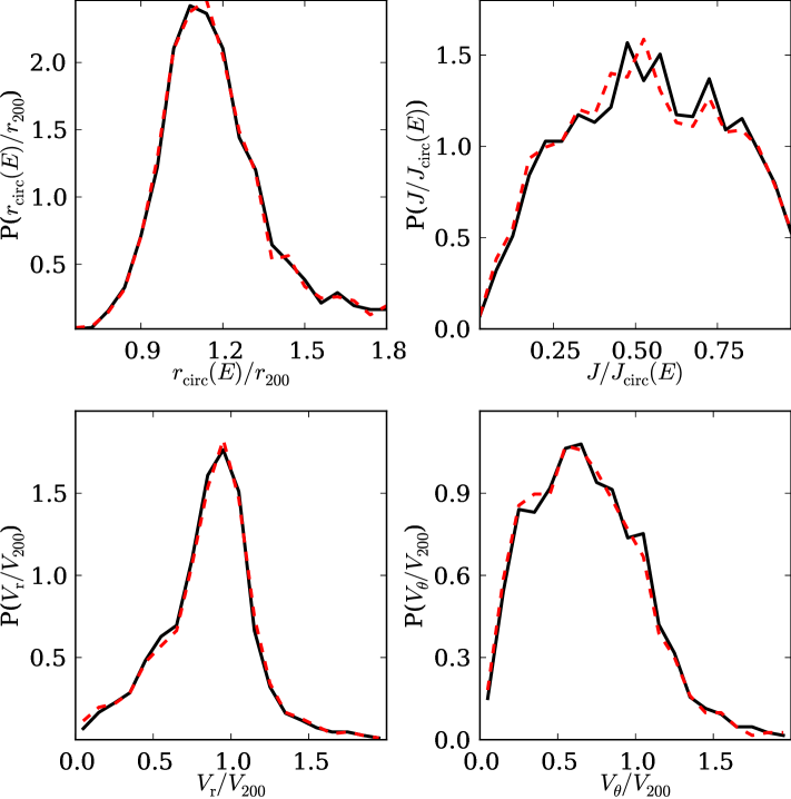
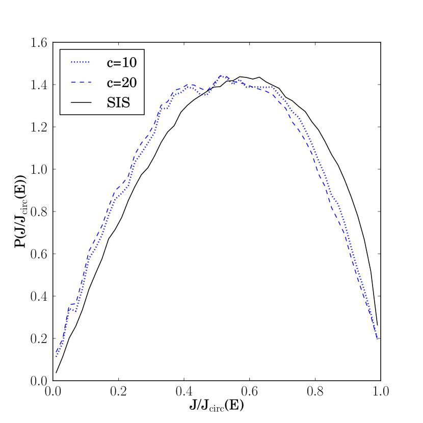
Provided our simulation snapshots are sufficiently closely spaced, we would expect these two methods to give very similar results. This is indeed what we find as demonstrated in Fig. 1 which compares the distribution of the various orbital parameters for satellites satisfying $M_{\rm s}/M_{\rm h}>0.05$ at the time of infall in our full sample of haloes. Throughout the rest of this paper, we show results just from the method that linearly interpolates the energy and angular momentum. We would expect this to be the more accurate method as these two quantities are almost conserved and so only vary slowly with the interpolation parameter.

Accurately defining the orbital parameters at the crossing time is an important issue that has been considered in earlier work. The approach adopted by Benson (2005) and Vitvitska et al. (2002) was to search for pairs of haloes within some separation $r_{\rm max}$ which are about to merge and then predict their crossing time by modelling them as two isolated point masses. A similar approach was taken by Tormen (1997), Khochfar & Burkert (2006) and Wetzel (2011). When using such schemes one must apply a weighting to correct for the under-representation of satellites with large infall velocities, some of which will be at separations greater than $r_{\rm max}$ at the earlier snapshot. In our work, due to the higher time resolution of our simulation outputs, we do not have to limit the separation between satellite and host halo at the snapshot prior to infall and instead form a complete census of all the infalling satellites.

Figure 2: The distributions of halo formation redshifts and the redshifts at which satellites fall into these halos. Each column is for a fixed final halo mass as labelled at the top of the figure. The top row is the distribution of halo formation redshifts. The middle row is the distribution of satellite infall redshifts for all infalling satellites, while bottom row is for the subset of these satellites which survive as subhaloes at $z=0$. In the bottom two rows the line colour indicates the satellite-to-host mass ratio. The red lines are for $0.0001<M_{\rm s}/M_{\rm h}<0.005$, green for $0.005<M_{\rm s}/M_{\rm h}<0.05$ and blue for $M_{\rm s}/M_{\rm h}>0.05$.

Figure 3: Comparison to published distributions of the orbital parameters $r_{\rm circ}(E)/r_{\rm 200}$, $J/J_{\rm circ}(E)$, $V_{\rm r}/V_{\rm 200}$, and $V_{\rm\theta}/V_{\rm 200}$. In all the panels the black solid line shows the distribution of the satellite orbital parameters for infalling satellites in our analysed host haloes (covering the mass range $5\times 10^{11}$ to $2.5\times 10^{14}$ M_⊙) with satellite-to-host halo mass ratios spanning $0.05$ to $0.5$. This range is typical of that probed by the samples to which we are comparing. Blue, green and red dashed lines show the results from the work of Tormen (1997), Wetzel (2011) and Benson (2005) respectively.

2.4 Formation and infall redshifts

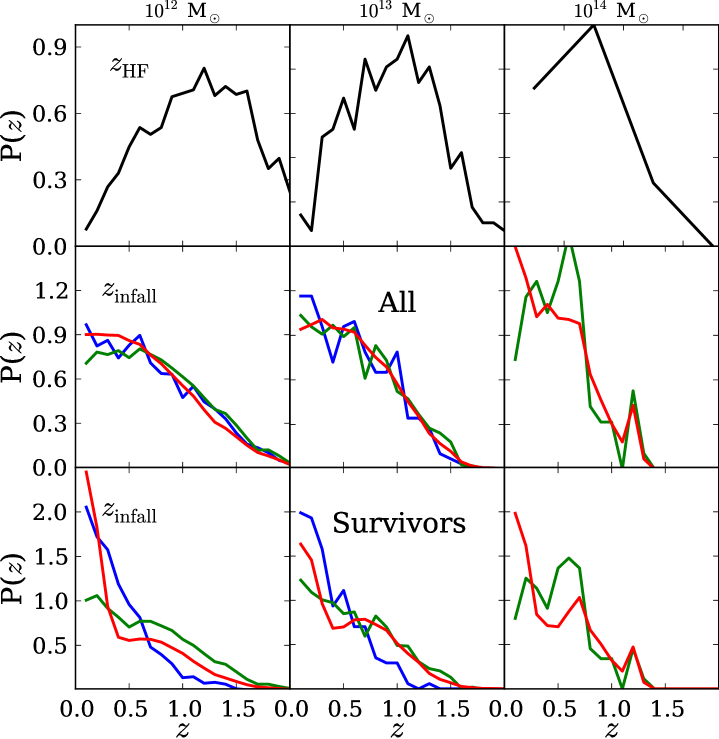
As we want our measured orbital parameter distributions to be directly applicable to semi-analytic galaxy formation models we trace all the infalling subhaloes back to the formation time of the main halo, where its formation time is defined as when its main progenitor has half the final, $z=0$, halo mass. We bin our halo samples by their mass at redshift $z=0$ and so by not tracing haloes back further in time we avoid significant ambiguity in the mass of the main halo at the time satellites are accreted, i.e. at all infall events the main halo is always within a factor of two the final halo mass. The probability distribution function of halo formation redshifts, $z_{\rm HF}$, (normalized such that the integral over the distribution is unity) are shown in the top row of Fig. 2 for each of our final halo mass bins. As expected we see that lower mass haloes form earlier. The median formation redshift of our $10^{12}$, $10^{13}$ and $10^{14}$ M_⊙ haloes are 1.14, 0.92, and 0.66 respectively.

The middle row of Fig. 2 shows the distribution of infall redshifts, $z_{\rm infall}$, split both by final halo mass and by the ratio of satellite-to-host mass at infall. These distributions rise steadily towards redshift $z=0$ (though the distributions for the highest mass bin are noisy because of the limited size of that sample) from the upper redshift set by when the first haloes in the sample form. The most interesting aspect is that infall redshift distribution at fixed halo mass is essentially independent of satellite-to-host mass ratio. This is equivalent to the mass distribution of the infalling satellites, measured in units of the host halo mass, being independent of redshift. Given that the distribution of host halo masses is constrained not to vary greatly with redshift (only haloes with mass greater than half the final mass are retained in the sample) then this behaviour is expected in simple excursion set models of hierarchical growth (Lacey & Cole, 1993).

Table 1: The median values of infall redshifts for both all and surviving subhaloes and the orbital parameter, $\log_{10}\Theta$ for bins of final halo mass, $M_{\rm h}$, and the satellite-to-host mass ratio at infall, $M_{\rm s}/M_{\rm h}$. The errors were estimated by bootstrap resampling of the halo sample.

$M_{\rm h}$	$M_{\rm s}/M_{\rm h}$	$\log_{10}\Theta$	$z_{\rm infall}$ survivors	$z_{\rm infall}$ all
1012 M⊙	$0.0001-0.005$	$\hphantom{-}0.076\pm{0.002}$	$0.217\pm{0.006}$	$0.491\pm{0.007}$
1013 M⊙	$0.0001-0.005$	$\hphantom{-}0.051\pm{0.004}$	$0.428\pm{0.025}$	$0.516\pm{0.017}$
1014 M⊙	$0.0001-0.005$	$\hphantom{-}0.050\pm{0.017}$	$0.380\pm{0.064}$	$0.409\pm{0.053}$
1012 M⊙	$0.005-0.05$	$\hphantom{-}0.027\pm{0.003}$	$0.462\pm{0.009}$	$0.521\pm{0.010}$
1013 M⊙	$0.005-0.05$	${-}0.009\pm{0.012}$	$0.480\pm{0.024}$	$0.522\pm{0.022}$
1014 M⊙	$0.005-0.05$	${-}0.015\pm{0.047}$	$0.483\pm{0.086}$	$0.483\pm{0.062}$
1012 M⊙	$0.05-0.5$	${-}0.082\pm{0.007}$	$0.290\pm{0.012}$	$0.511\pm{0.019}$
1013 M⊙	$0.05-0.5$	${-}0.130\pm{0.021}$	$0.268\pm{0.031}$	$0.484\pm{0.040}$

The bottom row of Fig. 2 also shows distributions of infall redshifts, but now just for the satellites that survive and are identifiable at redshift $z=0$. The median redshifts of these distributions are compared to those of corresponding complete samples in Table 1. Comparing these values and the distributions shown in the bottom and middle rows of Fig. 2 one clearly sees that the typical infall redshift of surviving satellites is significantly lower than that of the complete sample.

This is, at least in part, a resolution effect as we are unable to identify satellites with fewer than 20 particles. Thus the shift to lower infall redshifts is greatest for the lowest mass satellites which are the ones with the smaller satellite-to-host mass ratio in the lower halo mass bins.

3 Orbital Parameter Distributions

3.1 Comparison to previous work

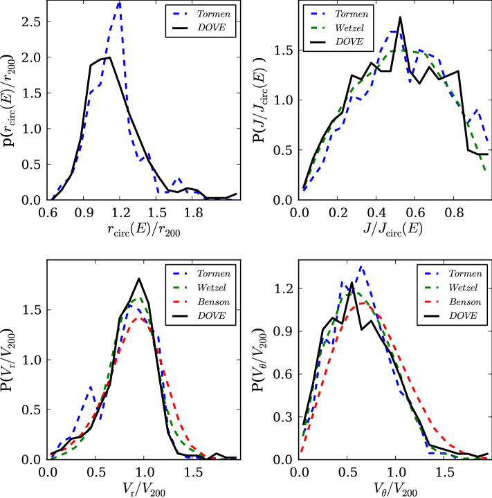
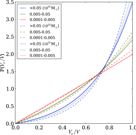
Fig. 3 compares our orbital parameter distributions with those from Tormen (1997), Benson (2005) and Wetzel (2011). In all panels, the black solid lines show the distributions for satellites with mass ratios in the range $0.05<M_{\rm s}/M_{\rm h}<0.5$ averaged over all our analysed haloes which span the mass range $5\times 10^{11}<M_{\rm h}<2.5\times 10^{14}$M_⊙. In general our results are in good agreement with these published datasets and those of Wang et al. (2005); Zentner et al. (2005); Khochfar & Burkert (2006), despite variations between these studies in the definition of crossing time and the choice of cosmology.

Figure 4: Orbital parameter distributions for bins of different final halo masses and satellite-to-host halo mass ratios, $M_{\rm s}/M_{\rm h}$. The central value of the final halo mass bin is indicated at the top of each column, with the rightmost column overplotting the results from each of the three mass bins using the appropriate line type. The red lines are for $0.0001<M_{\rm s}/M_{\rm h}<0.005$, green for $0.005<M_{\rm s}/M_{\rm h}<0.05$ and blue for $M_{\rm s}/M_{\rm h}>0.05$. The first two rows show the radial, $V_{r}/V_{\rm 200}$, and tangential, $V_{\rm\theta}/V_{\rm 200}$, velocity distributions. The second two rows show the circularity, $J/J_{\rm circ}(E)$, and $r_{\rm circ}(E)/r_{200}$, while the final row shows the distributions of the composite parameter $\Theta$ defined in Eqn. 7. Note that for host haloes in the 10¹⁴ M_⊙ bin, we do not show the $M_{\rm s}/M_{\rm h}>0.05$ distributions due to the low number of subhaloes.

The selection of Tormen (1997) data which we plot matches the $M_{\rm s}/M_{\rm h}>0.05$ cut used in our own data, but is for host halos with typical masses of $10^{15}$ M_⊙. The good agreement we find with Tormen (1997) is only expected if, as we find below, the distributions depend only weakly on halo mass at fixed $M_{\rm s}/M_{\rm h}$. The Benson (2005) data is based on a wide range of simulations of different volumes and resolutions. In this sample he uses all satellites and haloes with masses greater than $10^{11}$ M_⊙ and states that the typical ratio $M_{\rm s}/M_{\rm h}=0.08$. The smooth radial and tangential velocity distributions we plot in the lower panels of Fig. 3 are the fitted distributions presented by Benson (2005). Benson (2005) and also Vitvitska et al. (2002) modelled the radial distribution as a Gaussian and the tangential distribution as a Rayleigh or 2D Maxwell-Boltzmann distribution. The agreement with our results is reasonable. The radial and tangential velocity distributions of Wetzel (2011) are in very good agreement with our results. Like Benson, Wetzel uses all satellites and haloes above a fixed mass cut, $10^{10}$ M_⊙, and so we would expect the mean $M_{\rm s}/M_{\rm h}$ ratio to be similar to that of Benson and to our $0.05<M_{\rm s}/M_{\rm h}<0.5$ sample. The comparison of $J/J_{\rm circ}(E)$ distributions between us and Wetzel is not strictly fair as we compute $J_{\rm circ}(E)$ using the singular isothermal sphere model while he models the satellite and host as two point masses. However while this introduces a bias for satellites for which $M_{\rm s}/M_{\rm h}\ll 1$, we find that the resulting distributions are very similar for satellites with $0.05<M_{\rm s}/M_{\rm h}<0.5$ (see Appendix A).

Figure 5: The bivariate distributions of orbital parameters for all satellites infalling onto $10^{13}$ M_⊙ haloes. The top panels show the two-dimensional distribution of $r_{\rm circ}(E)/r_{\rm 200}$ versus $J/J_{\rm circ}(E)$ and $V_{\rm\theta}/V_{\rm 200}$ versus $V_{\rm r}/V_{\rm 200}$ respectively. The bottom panels show the two-dimensional distributions of $V/V_{\rm 200}$ versus $V_{r}/V_{\rm 200}$ and $V/V_{\rm 200}$ versus $V_{\theta}/V_{\rm 200}$. The colour bar illustrates the relative density of points (on an arbitrary scale).

Table 2: Parameters of the fitted orbital parameter distributions for bins of final halo mass, $M_{\rm h}$, and the satellite-to-host mass ratio at infall, $M_{\rm s}/M_{\rm h}$. The notation for the parameters of the Voigt and exponential fitting functions are as defined in Eqns. 11 and 12.

Mh	Ms/ Mh	$B$	$\gamma$	$\sigma$	$\mu$
1012 M⊙	$0.0001-0.005$	$0.049\pm{0.055}$	$\hphantom{-}0.109\pm{0.003}$	$0.077\pm{0.002}$	$1.220\pm{0.001}$
1013 M⊙	$0.0001-0.005$	$0.548\pm{0.105}$	$\hphantom{-}0.114\pm{0.010}$	$0.094\pm{0.006}$	$1.231\pm{0.002}$
1014 M⊙	$0.0001-0.005$	$1.229\pm{0.292}$	$\hphantom{-}0.110\pm{0.018}$	$0.072\pm{0.007}$	$1.254\pm{0.010}$
1012 M⊙	$0.005-0.05$	$1.044\pm{0.086}$	$\hphantom{-}0.098\pm{0.005}$	$0.073\pm{0.004}$	$1.181\pm{0.002}$
1013 M⊙	$0.005-0.05$	$1.535\pm{0.255}$	$\hphantom{-}0.087\pm{0.013}$	$0.083\pm{0.010}$	$1.201\pm{0.005}$
1014 M⊙	$0.005-0.05$	$3.396\pm{1.040}$	$\hphantom{-}0.050\pm{0.023}$	$0.118\pm{0.025}$	$1.236\pm{0.020}$
1012 M⊙	$0.05-0.5$	$2.878\pm{0.200}$	$\hphantom{-}0.071\pm{0.010}$	$0.091\pm{0.007}$	$1.100\pm{0.004}$
1013 M⊙	$0.05-0.5$	$3.946\pm{0.578}$	$\hphantom{-}0.030\pm{0.030}$	$0.139\pm{0.021}$	$1.100\pm{0.013}$
1014 M⊙	$0.05-0.5$	$2.982\pm{4.646}$	$-0.012\pm{0.035}$	$0.187\pm{0.019}$	$1.084\pm{0.052}$

3.2 Orbital parameters: mass ratio and mass dependence

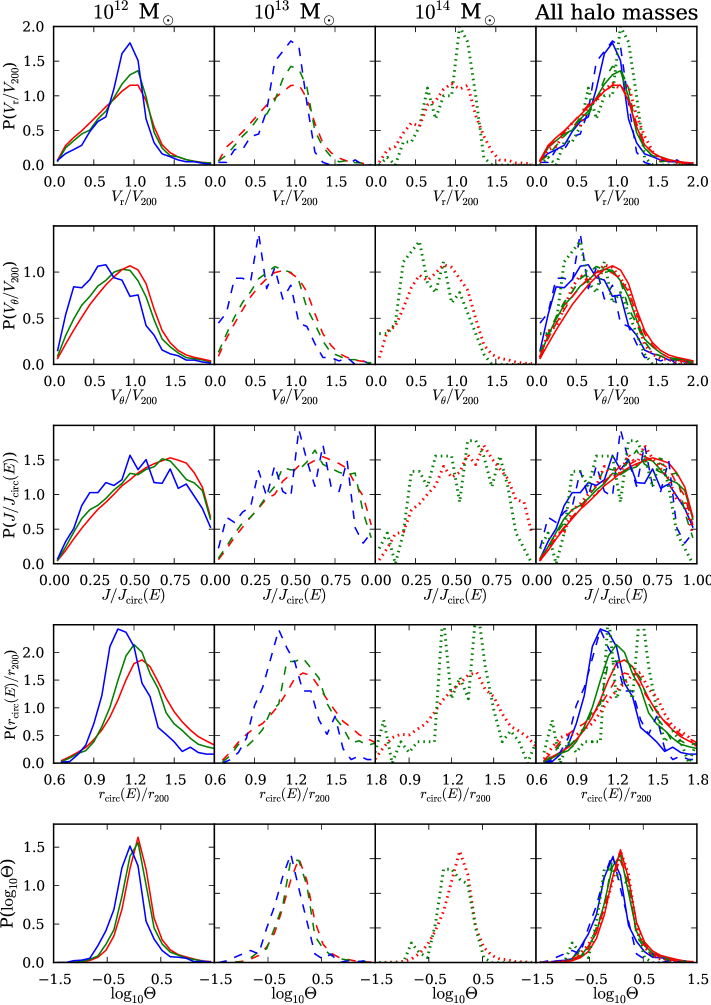
Fig 4 presents our results for the orbital parameter distributions for three bins of halo mass and three bins of satellite-to-host halo mass ratio. We reiterate that the host halo mass bins are defined by the mass of the host haloes at $z=0$ while the mass ratio, $M_{\rm s}/M_{\rm h}$, is defined by the values at the infall redshift.

The top two rows of Fig. 4 show the distributions of radial and tangential velocities at infall. The radial distributions peak close $V_{\rm r}=V_{200}$ and the tangential distributions at a lower value of around $V_{\theta}=0.65\,V_{200}$. As very few satellites are on unbound orbits, both distributions only have small tails beyond $1.5\,V_{200}$. Independently of host halo mass, we see that the distributions of radial velocities become broader for lower mass satellites with little change in the location of the peak of the distribution. In contrast for the tangential velocities the mode of the distribution shifts to higher values for less massive satellites. The most massive satellites are on the most radial, low angular momentum, orbits, The dependence of these distributions on halo mass at fixed $M_{\rm s}/M_{\rm h}$ is much weaker. This can be seen in the righthand panels where, to a first approximation, the lines of the same colour (same $M_{\rm s}/M_{\rm h}$) coincide. There is some residual dependence on halo mass (different line styles), with orbits becoming more radial – the $V_{\theta}/V_{200}$ distributions peaking at lower values – for more massive haloes, but this trend is much weaker.

The middle row of Fig. 4 shows the distributions of circularity, $J/J_{\rm circ}(E)$. The distributions are broad with those for the $M_{\rm s}/M_{\rm h}>0.05$ bin peaking at close to a circularity of a half. In each bin of halo mass, we again see the trend, for higher mass satellites to have less circular, more radially biased orbits. Also, once again, the trends with satellite-to-halo mass ratio are much stronger than those with halo mass.

The penultimate row of Fig. 4 shows the distributions of $r_{\rm circ}(E)/r_{200}$. This is essentially a measure of the energies of the orbits, with higher $r_{\rm circ}(E)/r_{200}$ corresponding to less bound orbits. At each halo mass, there is a strong trend for the more massive satellites to be more strongly bound. Again, the variations of the distributions with halo mass, at fixed satellite-to-halo mass ratio, are much weaker.

These trends are consistent with the picture put forward by Libeskind et al. (2005) that within the filaments of the cosmic web that surround an accreting dark matter halo, the most massive infalling haloes move along the central spines of the filaments. In this way the filamentary structures act as focusing rails which direct massive satellites onto predominantly radial orbits. Perhaps more simply, the force on the most massive satellites is dominated by the central halo while lower mass satellites can be significantly perturbed by other more massive satellites.

We show the distribution of the composite orbital parameter $\Theta$ in the bottom row of Fig. 4 and list their median values in Table 1. We see a clear shift in the distributions towards higher values of $\Theta$ with decreasing values of $M_{\rm s}/M_{\rm h}$ and weaker dependence on host halo mass. According to Eqn. 8 this will contribute to lower mass satellites having longer merger timescales but this effect is subdominant to the explicit $M_{\rm h}/M_{\rm s}$ term in that equation which also acts in the same sense.

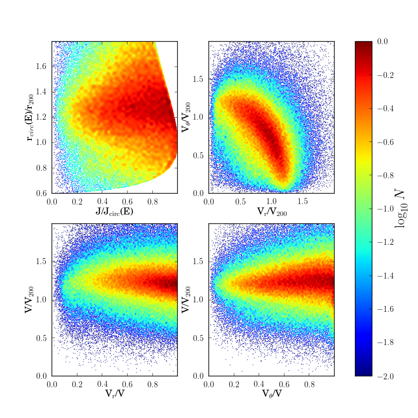
3.3 2D distribution of orbital parameters

As described in the Benson (2005) paper, the radial and tangential velocity distributions are tightly correlated. Consequently the 1-dimensional distributions presented in Fig. 4 are not a sufficient characterisation of the orbital parameter distributions. We emphasise this in Fig. 5 which shows bivariate distributions of various orbital parameter combinations.

The top left-hand panel of Fig. 5 shows the bivariate distribution of $r_{\rm circ}(E)/r_{200}$ and $J/J_{\rm circ}(E)$. The first thing to note in this distribution is that there are excluded regions at high value of $J/J_{\rm circ}(E)$ both for low and high values of $r_{\rm circ}(E)/r_{200}$. These arise from our stipulation that we are characterising the orbits of satellites when they first cross $r_{200}$. The plotted distribution touches the right hand axis at $r_{\rm circ}(E)/r_{200}=1$ and $J/J_{circ}(E)=1$. This point corresponds to a circular orbit with $r=r_{200}$. Circular orbits of either larger or smaller radius would not be included in our sample as they never cross $r_{200}$. Hence, $r_{\rm circ}(E)/r_{200}$ either increases of decreases away from unity for increasingly eccentric orbits in our sample. This defines the complicated boundary to the measured bivariate distribution.

The top right-hand panel of Fig. 5 shows the correlated bivariate distribution of radial and tangential velocities. This is similar to that presented and parametrised in Benson (2005). We note that the ridge line of this distribution is approximately circular, i.e. it corresponds to a fixed total velocity $V=\left(V_{r}^{2}+V_{\theta}^{2}\right)^{1/2}$.

The lower two panels of Fig. 5 show the two dimensional distributions of the total velocity versus either the ratio $V_{r}/V$ or $V_{\theta}/V$. We see to a good approximation these pairs of parameters appear uncorrelated. This suggests that we can construct a simple model for the full bivariate distribution of orbital parameters by modelling the individual independent distributions of $V/V_{200}$ and $V_{r}/V$. This will then provide a simple parametrised model that can be used in semi-analytic galaxy formation models.

3.4 Fitted Distributions

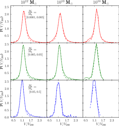
To build a complete model of the bivariate distribution of orbital parameters we perform fits to the marginalised distributions of both the total velocity, $V/V_{200},$ and the radial-to-total velocity ratio, $V_{r}/V$. Assuming these to be independent we can then transform variables to generate model predictions for the distributions of any of the other choices of orbital parameters such as $J/J_{\rm circ}(E)$ and $r_{\rm circ}(E)/r_{200}$. Here we present these fits as a function of halo mass and satellite-to-halo mass ratio.

The distributions of $V/V_{200}$ for each of our samples are shown in Fig. 6 along with Voigt profile fits. The distributions of $V/V_{200}$ are reasonably symmetric about their means but much more centrally peaked than Gaussians of the same rms width (leptokurtic). We find that the distributions can be fitted well by Voigt profiles, convolutions of a Lorentz profile,

$$P_{L}(x;\gamma)\equiv\frac{\gamma}{\pi(x^{2}+\gamma^{2})},$$ (9)

and a Gaussian

$$P_{G}(x;\sigma,\mu)\equiv\frac{1}{\sqrt{2\pi}\,\sigma}\exp\left(\frac{-(x-\mu)^{2}}{2\sigma^{2}}\right)$$ (10)

$$P_{V}(x;\sigma,\gamma,\mu)=\int_{-\infty}^{+\infty}P_{G}(x^{\prime};\sigma,\mu)P_{L}(x-x^{\prime};\gamma)dx^{\prime}$$ (11)

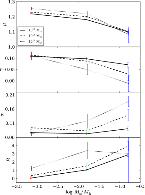
where $x=V/V_{200}$. We determine the best fitting Voigt profiles by finding the parameters that maximise the likelihood, ${\cal L}=\Pi_{i}P_{V}(x_{i};\sigma,\gamma,\mu)$, where the index $i$ runs over all the satellites in the sample. The resulting fits are shown in Fig. 6 and their parameters $\sigma$, $\gamma$ and $\mu$ are listed in Table. 2.

Figure 6: Probability distribution of the total infall velocity, $V/V_{200}$, as a function of both the satellite-to-host mass ratio at infall and the host halo mass. Each column is for a fixed final halo mass as labelled at the top of the column. Each row is for a different bin in satellite-to-host mass ratio: top (red lines) $0.0001<M_{\rm s}/M_{\rm h}<0.005$ , middle (green lines) $0.005<M_{\rm s}/M_{\rm h}<0.05$ and bottom (blue lines) $M_{\rm s}/M_{\rm h}>0.05$. The dashed lines are the Voigt profile fits whose parameters, $\mu$, $\gamma$ and $\sigma$ are listed in Table 2.

Figure 7: Dependence of the orbital parameters $V_{r}/V$ on the mass ratio between the satellite halo mass and the host halo mass. Each column is for a fixed final halo mass as labelled at the top of the figure. Each row is for a different bin in satellite-to-host mass ratio, top (red lines) $0.0001<M_{\rm s}/M_{\rm h}<0.005$, middle (green lines) $0.005<M_{\rm s}/M_{\rm h}<0.05$ and bottom (blue lines) $M_{\rm s}/M_{\rm h}>0.05$ The dashed curves are the best fitting exponential distributions and the corresponding value of the parameter $B$ in Eqn. 12) is shown on each panel and in Table 2.

Figure 8: The fitted distributions of the orbital parameters $V/V_{200}$ (top) and $V_{r}/V$ (bottom) for the different values of both the satellite-to-host mass ratio and the host halo mass. Line colour denotes satellite-to-host mass ratio, red $0.0001<M_{\rm s}/M_{\rm h}<0.005$, green $0.005<M_{\rm s}/M_{\rm h}<0.05$ and blue $M_{\rm s}/M_{\rm h}>0.05$. The line style indicates the host halo mass, solid $10^{12}$ M_⊙, dashed $10^{13}$ M_⊙ and dotted $10^{14}$ M_⊙.

Figure 9: Dependence of fitting parameters $\mu$, $\gamma$, $\sigma$ and $B$ on the satellite-to-host mass ratio at infall. Thetable different line styles denote different host halo masses, as indicated in the legend. The colours of the error bars denote satellite-to-host mass ratio bins: red $0.0001<M_{\rm s}/M_{\rm h}<0.005$, green $0.005<M_{\rm s}/M_{\rm h}<0.05$ and blue $M_{\rm s}/M_{\rm h}>0.05$. The errors are estimated by bootstrap sampling of the $z=0$ halo catalogue.

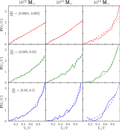
We find that the distributions $V_{r}/V$ are well fit by exponential distributions of the form:

$$P(V_{r}/V)=A\left(\exp\left(\frac{BV_{r}}{V}\right)-1\right).$$ (12)

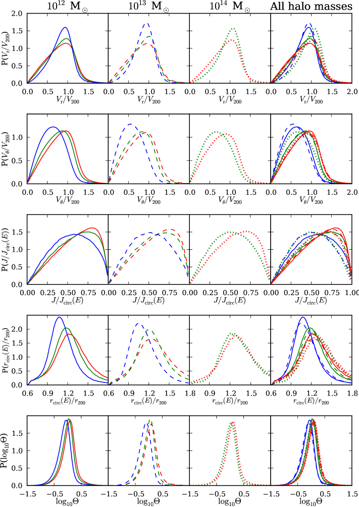
Here $A$ is simply a normalisation constant and $B$ is the single free parameter. The distributions of $V_{r}/V$ and the corresponding maximum likelihood fits are shown in Fig. 7. The distribution is almost linear, $B\ll 1$, for the combination of low $M_{\rm h}$ and low $M_{\rm s}/M_{\rm h}$. The distributions become increasingly radially biased, peaked at $V_{r}/V=1$ (high $B$), for both increasing $M_{\rm s}/M_{\rm h}$ and $M_{\rm h}$, consistent with our earlier discussion.

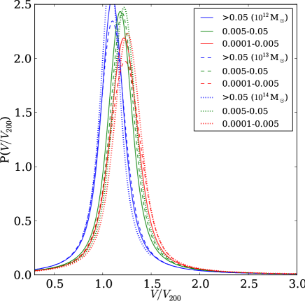
The trends of the distributions of $V/V_{200}$ and $V_{\rm r}/V$ with halo mass and satellite-to-halo mass ratio are depicted more clearly in Fig. 8, which shows all the fitted distributions on a single panel. In the lower panel we see the tendency for the distributions to become more radially biased for satellites with higher $M_{\rm s}/M_{\rm h}$. In the upper panel, it is clear that the $V/V_{200}$ distributions have very little dependence on halo mass at fixed $M_{\rm s}/M_{\rm h}$. There is a stronger dependence on $M_{\rm s}/M_{\rm h}$ with samples of larger $M_{\rm s}/M_{\rm h}$ ratios having narrower distributions and lower mean values. This is consistent with the similar trends in the distribution of $r_{\rm circ}(E)/r_{200}$ that we saw in Fig. 4. These trends can also be seen in Fig. 9, where we plot the dependence of the fit parameters on $M_{\rm s}/M_{\rm h}$. In all halo mass bins the mean, $\mu$, decreases strongly for the highest values of $M_{\rm s}/M_{\rm h}$. The narrower width of the $V/V_{200}$ distributions for high $M_{\rm s}/M_{\rm h}$, which we see in Fig. 8, is reflected in a decreasing value of $\gamma$ (the width of the Lorentzian) with increasing $M_{\rm s}/M_{\rm h}$, which has greater effect on the width of the distribution than the corresponding slow increase in $\sigma$ (the width of the Gaussian). The error bars shown on Fig. 9 have been estimated by bootstrap resampling of the $z=0$ halo catalogue and we have investigated the correlations of all the pairs of parameters. The only significant correlation we find is an anticorrelation between $\sigma$ and $\gamma$. This is to be expected as the overall width of the distribution is determined by $\sigma^{2}+\gamma^{2}$, while their ratio, $\gamma/\sigma$, determines how peaked the distribution is (its kurtosis).

3.5 Derived Distributions

If the fits we have presented in Section 3.4 are accurate and if $V_{r}/V$ and $V/V_{\rm 200}$ are uncorrelated then we can use these distributions to derive model distributions of any other choice of orbital parameter. For instance we can select pairs of values of $V_{r}/V$ and $V/V_{\rm 200}$ from the fitted distributions and compute the radial and tangential velocities using

$$\frac{V_{r}}{V_{200}}=\left(\frac{V_{r}}{V}\right)\left(\frac{V}{V_{200}}\right)$$ (13)

and

$$\frac{V_{\theta}}{V_{200}}=\left(\frac{V}{V_{200}}\right)\sqrt{1-\left(\frac{V_{r}}{V}\right)^{2}}.$$ (14)

We can also derive $J/J_{\rm circ}(E)$, $r_{\rm circ}(E)/r_{200}$ and $\Theta$ from $V_{r}/V$ and $V/V_{\rm 200}$ using the equations in Section 2.2. We show all the resulting orbital parameter distributions in Fig. 10, which should be compared with Fig. 4. Direct comparison of the two figures shows that these are faithful representations of the data and validate the assumption that, to a good approximation, $V_{r}/V$ and $V/V_{\rm 200}$ can be treated as independent random variables. The model distributions shown in Fig. 10, particularly the superimposed distributions in the righthand column, clearly show both the strong dependence on $M_{\rm s}/M_{\rm h}$ and the much weaker dependence on $M_{\rm h}$.

The values of $V$ and $V_{\rm r}$ are directly measured and so the fitted distributions of $V_{r}/V$ and $V/V_{\rm 200}$ make no assumption about the form of the density profile of the host halo. Hence if prefered one one can compute the corresponding orbital parameters $r_{\rm circ}(E)/r_{200}$ and $J/J_{\rm circ}(E)$ using an NFW model of the halo profile. Following the same steps as outlined in Section 2.2 but for an NFW profile one can show that $r_{\rm circ}(E)/r_{200}$ can be evaluated by solving

$$\frac{r_{\rm circ}(E)}{r_{200}}=\frac{2\ln(1+c\,r_{\rm circ}(E)/r_{200})-1/f(c\,r_{\rm circ}(E)/r_{200})}{2\ln(1+c)-V^{2}/(V_{200}^{2}f(c))}$$ (15)

where $f(c)=1/(\ln(1+c)-c/(c+1))$ and $c$ is the concentration. Having found $r_{c}(E)/r_{200}$, $J/J_{\rm circ}(E)$ can be found using

$$\frac{J}{J_{\rm circ}(E)}=\frac{V_{\theta}}{V_{200}}\left(\frac{f(c\,r_{\rm circ}(E)/r_{200})}{f(c)}\right)^{1/2}\left(\frac{r_{\rm circ}(E)}{r_{200}}\right)^{-1/2}.$$ (16)

Figure 10: Like Fig. 4, but showing the distributions derived from the fits presented in Section 3.4 rather than the directly measured distributions.

Figure 11: Comparison of the fitted distributions of orbital parameters $r_{\rm circ}(E)/r_{200}$, $J/J_{\rm circ}(E)$ for different assumed host halo density profiles. The black solid curve is for the default SIS profile when the blue dotted and dashed curves are for NFW profiles with concentrations $c=$10 and 20 respectively. This example is for host halo mass $M_{\rm h}=10^{12}$ M_⊙ and satellite to mass ratio in the range $0.05<M_{\rm s}/M_{\rm h}<0.5$.

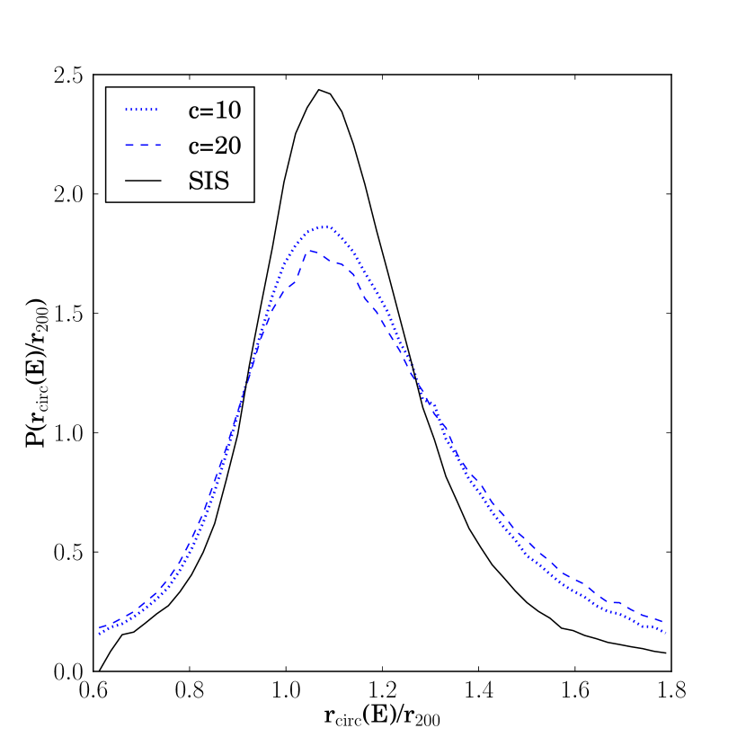
As an example, Fig. 11 compares the resulting distributions of $r_{\rm circ}(E)/r_{200}$ and $J/J_{\rm circ}(E)$ for host halo mass $M_{\rm h}=10^{12}$ M_⊙ and satellite to mass ratio in the range $0.05<M_{\rm s}/M_{\rm h}<0.5$. The NFW distributions of $r_{\rm circ}(E)/r_{200}$ are broader than the corresponding SIS distribution as over the relevant range $r_{\rm circ}(E)$ is a stronger function of energy in the NFW case than it is in the SIS case. The energy of a circular orbit at $r=r_{200}$ is the same for both NFW and SIS as both profiles are normalized to enclose the same mass, $M_{200}$, at this radius. As the orbital energy is increased $r_{\rm circ}(E)$ will grow faster for the NFW case as it has a more rapidly decreasing density profile. This leads to the enhanced tail of orbits with large $r_{\rm circ}(E)/r_{200}$. Higher concentration steepens the density profile around $r_{200}$ and so further enhances this tail, but this is a very weak effect. The $J/J_{\rm circ}$ distributions for the NFW models are slightly shifted to lower values. Since the measured values of $J$ do not depend on the model this shift is caused by the typical values of $J_{\rm circ}$ being larger in the NFW case. For a circular orbit at $r_{200}$ the NFW and SIS models have identical $J_{\rm circ}$ while at larger radii $J_{\rm circ}$ for a NFW prfile exceeds that for a SIS. Hence the small shift to lower $J/J_{\rm circ}$ is a result of this sample having a median value of $r_{\rm circ}(E)/r_{200}$ greater than unity. The shift is larger for lower mass satellites as their distributions of $r_{\rm circ}(E)/r_{200}$ have larger median values. The dependence on concentration is again very weak.

4 Conclusions

We have employed the DOVE high resolution cosmological N-body simulation with more than 4 billion particles to study the distribution of the orbits of infalling satellites during hierarchical halo formation in the standard $\Lambda$CDM cosmology. We study host haloes with masses from $10^{12}$ to $10^{14}$ M_⊙ and satellites with masses as low as $2\times 10^{8}$ M_⊙. Compared to previous studies (Tormen, 1997; Vitvitska et al., 2002; Benson, 2005; Wetzel, 2011) we have better mass and time resolution and a larger sample of satellite orbits.

There are various choices for the pair of orbital parameters that specify a satellite orbit in a spherical potential. We quantify the distributions of the radial, $V_{\rm r}$, and tangential, $V_{\theta}$, velocities as well as other common alternatives such as the circularity, $J/J_{\rm circ}(E)$ and the radius of the circular orbit of the same energy, $r_{\rm circ}(E)$.

We have examined the dependence of the distributions of these orbital parameters on both the host halo mass, $M_{\rm h}$, and the mass ratio between the satellite and host, $M_{\rm s}/M_{\rm h}$. We find that the strongest trends are with $M_{\rm s}/M_{\rm h}$ at fixed $M_{\rm h}$. Satellites with larger $M_{\rm s}/M_{\rm h}$ tend to be on more radial orbits with lower angular momentum and are more tightly bound. At fixed $M_{\rm s}/M_{\rm h}$ there is a trend for satellites around more massive haloes to also be on more radial orbits, but this trend is weaker. Insofar as previous authors have examined similar relationships, our results are consistent with their data. However, while Wetzel (2011) had not detected a significant dependence of orbital parameters on satellite mass ratio, possibly due to their limited sample size, our larger sample of orbits reveals a dependence, particularly at high mass ratios.

In general we find that complementary pairs of orbital parameters, such as ($V_{\rm r}$,$V_{\theta}$), are non-trivially correlated, making a complete description of their bivariate distribution complex. However, we find that, to a good approximation, the distributions of total infall velocity $V=(V_{\rm r}^{2}+V_{\theta}^{2})^{1/2}$ and the ratio $V_{r}/V$ are uncorrelated. We present accurate Voigt and exponential fits to their respective distributions. Assuming them to be uncorrelated, we transform these simple bivariate distributions and demonstrate that the distributions of other choices of orbital parameter can be successfully recovered.

Appendix A Circularity in the Keplerian Approximation

To compare the circularity, $J/J_{\rm circ}(E)$, inferred under the assumption that the infalling satellite and host halo are treated as two point masses on a Keplerian orbit with the singular isothermal sphere (SIS) model we need to compare the corresponding expressions for the angular momenta of circular orbits, $J_{\rm circ}(E)$. For the Keplerian case this is easily derived from the angular momentum of a circular orbit of radius $r$, $J_{\rm circ}=\mu V_{\rm circ}r$, where the circular velocity at separation $r$ is given by $\mu V_{\rm circ}^{2}=GM_{\rm h}M_{\rm s}/r$ and the corresponding orbital energy $E=\mu V_{\rm circ}^{2}/2-GM_{\rm h}M_{\rm s}/r$. Here $\mu$ is the reduced mass, which can be expressed in terms of the satellite and host masses as $\mu=M_{\rm s}M_{\rm h}/\left(M_{\rm s}+M_{\rm h}\right)$. Eliminating both $V_{\rm circ}$ and $r$ from these three equations yields

$$J^{\rm Kep}_{\rm circ}(E)=\sqrt{\frac{(GM_{\rm h}M_{\rm s})^{2}\mu}{-2E}}.$$ (17)

If $V$ is the velocity difference between the satellite and host when the satellite crosses the virial radius, $r_{200}$, then

$$E=\frac{1}{2}\mu V^{2}-\frac{GM_{\rm s}M_{\rm h}}{r_{200}}=\frac{1}{2}\mu V^{2}-M_{\rm s}V_{200}^{2},$$ (18)

where the circular velocity, $V_{200}$, is given by $V_{200}=\sqrt{GM_{\rm h}/r_{200}}$. Using Eqn. 18 to substitute for $E$ in Eqn. 17 yields

$$\frac{J^{\rm Kep}_{\rm circ}(E)}{M_{\rm s}V_{200}\,r_{200}}=\frac{1}{\sqrt{2M_{\rm s}/\mu-V^{2}/V_{200}^{2}}}.$$ (19)

This compares with the singular isothermal sphere expression for $J_{\rm circ}$ derived in Section 2.2,

$$\frac{J^{\rm SIS}_{\rm circ}(E)}{M_{\rm s}V_{200}\,r_{200}}=\exp\left(\frac{1}{2}\left(\frac{V^{2}}{V_{200}^{2}}-1\right)\right).$$ (20)

Figure 12: A comparison of the Keplerian and singular isothermal sphere (SIS) models of $J_{\rm circ}$ in units of $M_{\rm s}V_{200}\,r_{200}$ for satellites with infall velocity, $V$, at the virial radius $r_{200}$. In each panel, the black solid line is the SIS expression and the blue solid line is for the Keplerian case in the limit $M_{\rm s}/M_{\rm h}\ll 1$. The stars show the result of the full Keplerian expression including the dependence on the reduced mass, $\mu$, for for samples of satellites in different bins of $M_{\rm s}/M_{\rm h}$.

Figure 13: Distributions of circularity, $J/J_{\rm circ}(E)$, for infalling satellite haloes for host haloes in a mass bin centred on $10^{13}$ M_⊙. Solid curves show the distribution derived assuming a singular isothermal sphere and dashed curves show the distribution derived using the Keplerian model. The three panels are for the same three bins of $M_{\rm s}/M_{\rm h}$ as in Fig. 12.

The solid curves in Fig. 12 compare, as a function of satellite infall velocity, $V$, the SIS expression with the Keplerian expression evaluated in the limit $M_{\rm s}/M_{\rm h}\ll 1$, such that $\mu\rightarrow M_{\rm s}$. The individual points on the different panels show the results of the full Keplerian expression with its dependence on $M_{\rm s}/\mu$ applied to our satellite sample in different bins of $M_{\rm s}/M_{\rm h}$. The model curves necessarily agree at $V=V_{200}$ because the mass enclosed in a circular orbit at $r_{200}$, where the circular velocity is $V_{200}$, is the same by construction. For $M_{\rm s}/M_{\rm h}\ll 1$, the difference between the two models is largest at large $V/V_{200}$ where the orbits extend far beyond $r_{200}$ and hence the mass enclosed in the SIS greatly exceeds the mass assumed in the point mass approximation. The effect of the reduced mass, $\mu$, is small for $M_{\rm s}/M_{\rm h}<0.05$, but for $0.05<M_{\rm s}/M_{\rm h}<0.5$ it has the effect of reducing $J^{\rm Kep}_{\rm circ}(E)$ and produces values closer to the SIS case. This is demonstrated in Fig. 13 which compares the distribution of circularities, $J/J_{\rm circ}(E)$, evaluated using the two different expressions for three ranges in satellite-to-host mass ratio. Overall, the two models agree well with each other for higher values of $M_{\rm s}/M_{\rm h}$, but they differ for the lowest mass ratio bins.

References

- Baugh (2006) Baugh C. M., 2006, Reports on Progress in Physics, 69, 3101
- Benson (2005) Benson A. J., 2005, MNRAS, 358, 551
- Binney & Tremaine (2008) Binney J., Tremaine S., 2008, Galactic Dynamics: Second Edition. Princeton University Press
- Boylan-Kolchin et al. (2008) Boylan-Kolchin M., Ma C.-P., Quataert E., 2008, MNRAS, 383, 93
- Chandrasekhar (1943) Chandrasekhar S., 1943, ApJ, 97, 255
- Cole & Lacey (1996) Cole S., Lacey C., 1996, MNRAS, 281, 716
- Davis et al. (1985) Davis M., Efstathiou G., Frenk C. S., White S. D. M., 1985, ApJ, 292, 371
- Gill et al. (2004) Gill S. P. D., Knebe A., Gibson B. K., Dopita M. A., 2004, MNRAS, 351, 410
- Jenkins (2010) Jenkins A., 2010, MNRAS, 403, 1859
- Jenkins (2013) Jenkins A., 2013, MNRAS, 434, 2094
- Jiang et al. (2008) Jiang C. Y., Jing Y. P., Faltenbacher A., Lin W. P., Li C., 2008, ApJ, 675, 1095
- Jiang et al. (2014) Jiang L., Helly J. C., Cole S., Frenk C. S., 2014, MNRAS, 440, 2115
- Khochfar & Burkert (2006) Khochfar S., Burkert A., 2006, A&A, 445, 403
- Klypin et al. (1999) Klypin A., Gottlöber S., Kravtsov A. V., Khokhlov A. M., 1999, ApJ, 516, 530
- Komatsu et al. (2011) Komatsu E., Smith K. M., Dunkley J., Bennett C. L., Gold B., Hinshaw G., Jarosik N., Larson D., Nolta M. R., Page L., et al. 2011, ApJS, 192, 18
- Lacey & Cole (1993) Lacey C., Cole S., 1993, MNRAS, 262, 627
- Libeskind et al. (2005) Libeskind N. I., Frenk C. S., Cole S., Helly J. C., Jenkins A., Navarro J. F., Power C., 2005, MNRAS, 363, 146
- Moore et al. (1999) Moore B., Ghigna S., Governato F., Lake G., Quinn T., Stadel J., Tozzi P., 1999, ApJ, 524, L19
- Navarro et al. (1996) Navarro J. F., Frenk C. S., White S. D. M., 1996, ApJ, 462, 563
- Schaye et al. (2014) Schaye J., Crain R. A., Bower R. G., Furlong M., Schaller M., Theuns T., Dalla Vecchia C., Frenk C. S., McCarthy I. G., Helly J. C., Jenkins A., Rosas-Guevara Y. M., White S. D. M., 2014, ArXiv e-prints
- Springel (2005) Springel V., 2005, MNRAS, 364, 1105
- Springel et al. (2001) Springel V., White S. D. M., Tormen G., Kauffmann G., 2001, MNRAS, 328, 726
- Tormen (1997) Tormen G., 1997, MNRAS, 290, 411
- Vitvitska et al. (2002) Vitvitska M., Klypin A. A., Kravtsov A. V., Wechsler R. H., Primack J. R., Bullock J. S., 2002, ApJ, 581, 799
- Wang et al. (2005) Wang H. Y., Jing Y. P., Mao S., Kang X., 2005, MNRAS, 364, 424
- Wetzel (2011) Wetzel A. R., 2011, MNRAS, 412, 49
- White & Rees (1978) White S. D. M., Rees M. J., 1978, MNRAS, 183, 341
- Zentner et al. (2005) Zentner A. R., Berlind A. A., Bullock J. S., Kravtsov A. V., Wechsler R. H., 2005, ApJ, 624, 505