Globally convergent and adaptive finite element methods in imaging of buried objects from experimental backscattering radar measurements

Larisa Beilina1111Corresponding author, Nguyen Trung Thành2, Michael V. Klibanov3
and John Bondestam Malmberg1
1Department of Mathematical Sciences,
Chalmers University of Technology and Gothenburg University,
SE-42196 Gothenburg, Sweden
Emails: larisa@chalmers.se, john.bondestam.malmberg@chalmers.se.
2Department of Mathematics, Iowa State University,
Ames, IA 50011, USA. Email: thanh@iastate.edu.
3Department of Mathematics & Statistics, University of North Carolina at Charlotte,
Charlotte, NC 28223, USA. Email: mklibanv@uncc.edu
Abstract

We consider a two-stage numerical procedure for imaging of objects buried in dry sand using time-dependent backscattering experimental radar measurements. These measurements are generated by a single point source of electric pulses and are collected using a microwave scattering facility which was built at the University of North Carolina at Charlotte. Our imaging problem is formulated as the inverse problem of the reconstruction of the spatially distributed dielectric permittivity εr(𝐱),𝐱3subscript𝜀r𝐱𝐱superscript3\varepsilon_{\mathrm{r}}\left(\mathbf{x}\right),\ \mathbf{x}\in\mathbb{R}^{3}, which is an unknown coefficient in Maxwell’s equations.

On the first stage an approximately globally convergent method is applied to get a good first approximation for the exact solution. On the second stage a local adaptive finite element method is applied to refine the solution obtained on the first stage. The two-stage numerical procedure results in accurate imaging of all three components of interest of targets: shapes, locations and refractive indices. In this paper we briefly describe methods and present new reconstruction results for both stages.

Keywords: Inverse scattering, refractive indices, approximately globally convergent algorithm, adaptive finite element method.

AMS classification codes: 65N15, 65N30, 35J25.

1 Introduction

In this paper we consider the problem of reconstruction of refractive indices, shapes and locations of buried objects in the dry sand from backscattering time-dependent experimental data using the two-stage numerical procedure presented in [6, 12, 14, 26]. Our problem is a coefficient inverse problem (CIP) for Maxwell’s equations in three dimensions. Experimental data were collected using a microwave scattering facility which was built at the University of North Carolina at Charlotte, USA. Our experimental data are collected using a single location of the source. The backscattered signal is measured on a part of a plane. Our potential applications are in the imaging of explosives, such as land mines and improvised explosive devices. This work is a continuation of our recent works on this topic, where we have treated a much simpler case of experimental data for targets placed in air [13, 14, 21].

The two-stage numerical procedure means that we combine two different methods to solve our CIP. On the first stage the approximately globally convergent method of [12] is applied in order to obtain a good first approximation for the exact solution. We have presented results of reconstruction on this stage in our publications [13, 21] for objects placed in air. In our recent study [22] we presented reconstructions of twenty-five objects which show that the method of [12] works well in estimating the dielectric constants (equivalently, refractive indices) and locations of buried objects.

In [3] it was investigated why a minimizer of the Tikhonov functional is indeed closer to the exact solution than the first guess of this minimizer. Because of that it makes sense improve the solution which we have obtained on the first stage of our two-stage numerical procedure. To do that the local adaptive finite element method of [10] is applied by taking the solution of the first stage as the starting point in the minimization of a Tikhonov functional in order to obtain better approximations and shapes of objects on the adaptively refined meshes. In [14] it was shown that using the adaptive finite element method all three components of interest for targets placed in the air can be simultaneously imaged: refractive indices, shapes and locations.

Compared to imaging of targets placed in the air (see [13, 14, 21]), there are three main difficulties in imaging of buried targets: (i) the signals of targets are much weaker than those when the targets are in air, (ii) these signals may overlap with the reflection from the ground’s surface, which makes them difficult to distinguish, and (iii) the reflection from the grounds surface may dominate the target’s signals after the Laplace transform since the kernel of the Laplace transform decays exponentially with respect to time. We have handled this difficulty in [22] via a new data preprocessing procedure. This procedure results in preprocessed data, which are used as the input for our globally convergent algorithm, that is, the input for the first stage of our method.

It is notable that we have experimentally observed a rare superresolution phenomenon and have numerically reconstructed the corresponding image (see section 7). The resolution limit which follows from the Born approximation, that is, in the diffraction limit, is λ/2𝜆2\lambda/2, where λ𝜆\lambda is the wavelength of the signal. However, we have resolved two targets with the distance λ/4.5𝜆4.5\lambda/4.5 between their surfaces. It was shown in, for instance [24], that the superresolution can occur because of nonlinear scattering, and our algorithm is nonlinear, including the step of extraction of the target’s signal in our data preprocessing procedure [22]. Experimentally the superresolution phenomenon was demonstrated in [17]. We also refer to the recent work [1] where the superresolution is discussed.

An outline of this paper follows. In section 2 we briefly describe the approximate globally convergent method. In section 3 we present the forward, inverse, and adjoint problems as well as the Tikhonov functional for the second stage. In section 4 we describe the finite element method used in computations and in section 5 we investigate general framework for a posteriori error estimation for CIPs. In section 6 we describe the mesh refinement recommendation and the adaptive algorithm. In section 7 we present results of our computations.

2 The first stage

In this section we state the forward and inverse problems which we consider on the first stage. We also briefly outline the globally convergent method of [12] and present the algorithm used in computations of the first stage.

2.1 Forward and inverse problems

Let Ω3Ωsuperscript3\Omega\subset\mathbb{R}^{3} be a convex bounded domain with the boundary ΩC3.Ωsuperscript𝐶3\partial\Omega\in C^{3}. Denote the spatial coordinates by 𝐱=(x,y,z)3.𝐱𝑥𝑦𝑧superscript3\mathbf{x}=\left(x,\,y,\,z\right)\in\mathbb{R}^{3}. Let Ck+αsuperscript𝐶𝑘𝛼C^{k+\alpha} be Hölder spaces, where k0𝑘0k\geq 0 is an integer and α(0, 1).𝛼01\alpha\in\left(0,\,1\right). We consider the propagation of the electromagnetic wave in 3superscript3\mathbb{R}^{3} generated by an incident plane wave. On the first stage we model the wave propagation by the following Cauchy problem for the scalar wave equation

εr(𝐱)2ut2(𝐱,t)Δu(𝐱,t)=δ(zz0)f(t),subscript𝜀r𝐱superscript2𝑢superscript𝑡2𝐱𝑡Δ𝑢𝐱𝑡𝛿𝑧subscript𝑧0𝑓𝑡\displaystyle{\varepsilon_{\mathrm{r}}}(\mathbf{x})\frac{\partial^{2}u}{\partial t^{2}}(\mathbf{x},\,t)-\Delta u(\mathbf{x},\,t)=\delta(z-z_{0})f(t), (𝐱,t)3×(0,),𝐱𝑡superscript30\displaystyle(\mathbf{x},\,t)\in\mathbb{R}^{3}\times(0,\,\infty), (1)
u(𝐱, 0)=0,ut(𝐱, 0)=0,formulae-sequence𝑢𝐱 00𝑢𝑡𝐱 00\displaystyle u(\mathbf{x},\,0)=0,\quad\frac{\partial u}{\partial t}(\mathbf{x},\,0)=0, 𝐱3.𝐱superscript3\displaystyle\mathbf{x}\in\mathbb{R}^{3}. (2)

Here f(t)0not-equivalent-to𝑓𝑡0f\left(t\right)\not\equiv 0 is the time-dependent incident plane wave at the plane {z=z0}𝑧subscript𝑧0\left\{z=z_{0}\right\}, u𝑢u is the total wave generated by f(t)𝑓𝑡f(t) and propagating along the z𝑧z-axis.

Let the function E(𝐱,t)𝐸𝐱𝑡E\left(\mathbf{x},\,t\right) represent the voltage of one component E2subscript𝐸2E_{2} of the electric field E(𝐱,t)=(E1,E2,E3)(𝐱,t).𝐸𝐱𝑡subscript𝐸1subscript𝐸2subscript𝐸3𝐱𝑡E\left(\mathbf{x},\,t\right)=\left(E_{1},\,E_{2},\,E_{3}\right)\left(\mathbf{x},\,t\right). In our experiments the component E2subscript𝐸2E_{2} corresponds to the electromagnetic wave which is sent into the medium. Our mathematical model of the first stage uses only the single equation (1) with u=E2𝑢subscript𝐸2u=E_{2} instead of the full Maxwell’s system. We can do such approximation since it was shown numerically in [9] that the component E2subscript𝐸2E_{2} of the electric field E𝐸E dominates the other two components in the case we consider. See also [12] where a similar scalar wave equation was used to work with transmitted experimental data.

The function εrsubscript𝜀r{\varepsilon_{\mathrm{r}}} in (1) represents the spatially distributed dielectric permittivity. We assume that εrsubscript𝜀r{\varepsilon_{\mathrm{r}}} is unknown inside the domain Ω3Ωsuperscript3\Omega\subset\mathbb{R}^{3} and is such that

εrCα(3),εr(𝐱)[1,b] for 𝐱3,εr(𝐱)=1 for 𝐱3Ω,formulae-sequenceformulae-sequencesubscript𝜀rsuperscript𝐶𝛼superscript3subscript𝜀r𝐱1𝑏 for 𝐱superscript3subscript𝜀r𝐱1 for 𝐱superscript3Ω\varepsilon_{\mathrm{r}}\in C^{\alpha}\left(\mathbb{R}^{3}\right),\quad\varepsilon_{\mathrm{r}}(\mathbf{x})\in[1,\,b]\text{ for }\mathbf{x}\in\mathbb{R}^{3},\quad\varepsilon_{\mathrm{r}}(\mathbf{x})=1\text{ for }\mathbf{x}\in\mathbb{R}^{3}\setminus\Omega, (3)

where b>1𝑏1b>1 is a constant. We assume that the set of admissible coefficients in (3) is known. Let ΓΩΓΩ\Gamma\subset\partial\Omega be a part of the boundary Ω.Ω\partial\Omega. In our experiments the plane wave is initialized outside of the domain Ω¯¯Ω\overline{\Omega}, that is Ω¯{z=z0}=¯Ω𝑧subscript𝑧0\overline{\Omega}\cap\{z=z_{0}\}=\varnothing.

Coefficient Inverse Problem (CIP). Determine the function εr(𝐱)subscript𝜀r𝐱\varepsilon_{\mathrm{r}}\left(\mathbf{x}\right) for 𝐱Ω𝐱Ω\mathbf{x}\in\Omega, assuming that the following function g𝑔g is known for a single incident plane wave generated at the plane {z=z0}𝑧subscript𝑧0\{z=z_{0}\} outside of Ω¯¯Ω\overline{\Omega}:

u(𝐱,t)=g(𝐱,t)(𝐱,t)Γ×(0,).𝑢𝐱𝑡𝑔𝐱𝑡for-all𝐱𝑡Γ0u\left(\mathbf{x},\,t\right)=g\left(\mathbf{x},\,t\right)~{}\forall\left(\mathbf{x},\,t\right)\in\Gamma\times\left(0,\,\infty\right).

Global uniqueness theorems for multidimensional CIPs with a single measurement are currently known only under the assumption that at least one of initial conditions does not equal zero in the entire domain Ω¯¯Ω\overline{\Omega} [12, 16]. However, this is not our case and the method of Carleman estimates is inapplicable to our CIP. Thus, we simply assume that uniqueness of our CIP holds.

2.2 The globally convergent method

Here we briefly present approximately globally convergent method of [12].

We perform a Laplace transformation

u~(𝐱,s)=0u(𝐱,t)estdt,~𝑢𝐱𝑠superscriptsubscript0𝑢𝐱𝑡superscript𝑒𝑠𝑡differential-d𝑡\tilde{u}(\mathbf{x},\,s)=\int\limits_{0}^{\infty}u(\mathbf{x},\,t)e^{-st}\,\mathrm{d}t,

where s𝑠s is a positive parameter which we call pseudo frequency. We assume that ss¯>0𝑠¯𝑠0s\geq\underline{s}>0 and denote by f~(s)~𝑓𝑠\tilde{f}(s) the Laplace transform of f(t)𝑓𝑡f(t). We assume that f~(s)0~𝑓𝑠0\tilde{f}(s)\neq 0 for all ss¯𝑠¯𝑠s\geq\underline{s}. Define w(𝐱,s):=u~(𝐱,s)/f~(s)assign𝑤𝐱𝑠~𝑢𝐱𝑠~𝑓𝑠w(\mathbf{x},\,s):=\tilde{u}(\mathbf{x},\,s)/\tilde{f}(s). The function w𝑤w satisfies the equation

Δw(𝐱,s)s2εr(𝐱)w(𝐱,s)=δ(zz0),𝐱3,ss¯.formulae-sequenceΔ𝑤𝐱𝑠superscript𝑠2subscript𝜀r𝐱𝑤𝐱𝑠𝛿𝑧subscript𝑧0formulae-sequence𝐱superscript3𝑠¯𝑠\Delta w(\mathbf{x},\,s)-s^{2}{\varepsilon_{\mathrm{r}}}(\mathbf{x})w(\mathbf{x},\,s)=-\delta(z-z_{0}),\quad\mathbf{x}\in\mathbb{R}^{3},\,\ s\geq\underline{s}. (4)

It was shown in [22] that w(𝐱,s)>0𝑤𝐱𝑠0w(\mathbf{x},\,s)>0 and lim|𝐱|[w(𝐱,s)w0(𝐱,s)]=0,subscript𝐱delimited-[]𝑤𝐱𝑠subscript𝑤0𝐱𝑠0\lim_{\left|\mathbf{x}\right|\rightarrow\infty}\left[w\left(\mathbf{x},\,s\right)-w_{0}(\mathbf{x},\,s)\right]=0, where w0(𝐱,s):=es|zz0|/(2s)assignsubscript𝑤0𝐱𝑠superscript𝑒𝑠𝑧subscript𝑧02𝑠w_{0}\left(\mathbf{x},\,s\right):=e^{-s\left|z-z_{0}\right|}/\left(2s\right) is a solution of equation (4) for the case εr(𝐱)1,subscript𝜀r𝐱1{\varepsilon_{\mathrm{r}}}\left(\mathbf{x}\right)\equiv 1, which decays to zero as |z|.𝑧\left|z\right|\rightarrow\infty. Next, introduce the function v𝑣v by v(𝐱,s):=ln(w(𝐱,s))/s2assign𝑣𝐱𝑠𝑤𝐱𝑠superscript𝑠2v(\mathbf{x},\,s):=\ln\big{(}w(\mathbf{x},\,s)\big{)}/s^{2} and substitute w=exp(vs2)𝑤𝑣superscript𝑠2w=\exp(vs^{2}) into (4). By noting that Ω¯{z=z0}=¯Ω𝑧subscript𝑧0\overline{\Omega}\cap\{z=z_{0}\}=\varnothing, we obtain the following equation for the explicit computation of the coefficient εrsubscript𝜀r{\varepsilon_{\mathrm{r}}}:

Δv(𝐱,s)+s2|v(𝐱,s)|2=εr(𝐱),𝐱Ω,ss¯.formulae-sequenceΔ𝑣𝐱𝑠superscript𝑠2superscript𝑣𝐱𝑠2subscript𝜀r𝐱formulae-sequence𝐱Ω𝑠¯𝑠\Delta v(\mathbf{x},\,s)+s^{2}|\nabla v(\mathbf{x},\,s)|^{2}={\varepsilon_{\mathrm{r}}}(\mathbf{x}),\quad\mathbf{x}\in\Omega,~{}s\geq\underline{s}. (5)

Next, we eliminate the unknown coefficient εr(𝐱)subscript𝜀r𝐱{\varepsilon_{\mathrm{r}}}(\mathbf{x}) from (5) by taking the derivative with respect to s𝑠s both sides of (5). Denote by q:=vsassign𝑞𝑣𝑠q:=\frac{\partial v}{\partial s}, then

v(𝐱,s)=sq(𝐱,τ)dτ=ss¯q(𝐱,τ)dτ+V(𝐱),𝑣𝐱𝑠superscriptsubscript𝑠𝑞𝐱𝜏differential-d𝜏superscriptsubscript𝑠¯𝑠𝑞𝐱𝜏differential-d𝜏𝑉𝐱v(\mathbf{x},\,s)=-\int\limits_{s}^{\infty}q(\mathbf{x},\,\tau)\,\mathrm{d}\tau=-\int\limits_{s}^{\bar{s}}q(\mathbf{x},\,\tau)\,\mathrm{d}\tau+V(\mathbf{x}),

where s¯>s¯¯𝑠¯𝑠\bar{s}>\underline{s}. We call the function V(𝐱)=v(𝐱,s¯)𝑉𝐱𝑣𝐱¯𝑠V(\mathbf{x})=v(\mathbf{x},\,\bar{s}) the “tail function”and define it by

V(𝐱)=lnw(𝐱,s¯)s¯2.𝑉𝐱𝑤𝐱¯𝑠superscript¯𝑠2V(\mathbf{x})=\frac{\ln w(\mathbf{x},\,\bar{s})}{\bar{s}^{2}}. (6)

From (5) we obtain the following equation for two unknown functions q𝑞q and V𝑉V

Δq(𝐱,s)Δ𝑞𝐱𝑠\displaystyle\Delta q(\mathbf{x},\,s) 2s2q(𝐱,s)ss¯q(𝐱,τ)dτ+2s2V(𝐱)q(𝐱,s)2superscript𝑠2𝑞𝐱𝑠superscriptsubscript𝑠¯𝑠𝑞𝐱𝜏differential-d𝜏2superscript𝑠2𝑉𝐱𝑞𝐱𝑠\displaystyle-2s^{2}\nabla q(\mathbf{x},\,s)\cdot\int\limits_{s}^{\bar{s}}\nabla q(\mathbf{x},\,\tau)\,\mathrm{d}\tau+2s^{2}\nabla V(\mathbf{x})\cdot\nabla q(\mathbf{x},\,s) (7)
+2s|ss¯q(𝐱,τ)dτ|24sV(𝐱)ss¯q(𝐱,τ)dτ+2s|V(𝐱)|2=0,2𝑠superscriptsuperscriptsubscript𝑠¯𝑠𝑞𝐱𝜏differential-d𝜏24𝑠𝑉𝐱superscriptsubscript𝑠¯𝑠𝑞𝐱𝜏differential-d𝜏2𝑠superscript𝑉𝐱20\displaystyle+2s\left|\int\limits_{s}^{\bar{s}}\nabla q(\mathbf{x},\,\tau)\,\mathrm{d}\tau\right|^{2}-4s\nabla V(\mathbf{x})\cdot\int\limits_{s}^{\bar{s}}\nabla q(\mathbf{x},\,\tau)\,\mathrm{d}\tau+2s\left|\nabla V(\mathbf{x})\right|^{2}=0,

for 𝐱Ω𝐱Ω\mathbf{x}\in\Omega and s(s¯,s¯)𝑠¯𝑠¯𝑠s\in(\underline{s},\,\bar{s}).

To find the tail function V𝑉V we use an iterative procedure presented in the next section, see [13, 21] for details of this procedure. The function q𝑞q satisfies the following boundary condition

q(𝐱,s)=ψ(𝐱,s),𝐱Ω,formulae-sequence𝑞𝐱𝑠𝜓𝐱𝑠𝐱Ωq(\mathbf{x},\,s)=\psi(\mathbf{x},\,s),\quad\mathbf{x}\in\partial\Omega, (8)

where ψ(𝐱,s)=s[lnφ(𝐱,s)s2]𝜓𝐱𝑠𝑠delimited-[]𝜑𝐱𝑠superscript𝑠2\psi(\mathbf{x},\,s)=\frac{\partial}{\partial s}\left[\frac{\ln\varphi(\mathbf{x},\,s)}{s^{2}}\right] with φ(𝐱,s)=0g(𝐱,t)estdt/f~(s)𝜑𝐱𝑠superscriptsubscript0𝑔𝐱𝑡superscript𝑒𝑠𝑡differential-d𝑡~𝑓𝑠\varphi(\mathbf{x},\,s)=\int\limits_{0}^{\infty}g(\mathbf{x},\,t)e^{-st}\,\mathrm{d}t/\tilde{f}(s).

2.3 Iterative procedure and description of the approximate globally convergent algorithm

In our iterative procedure we divide the pseudo frequency interval [s¯,s¯]¯𝑠¯𝑠[\underline{s},\,\bar{s}] into N𝑁N sub-intervals s¯=s0>s1>>sN=s¯¯𝑠subscript𝑠0subscript𝑠1subscript𝑠𝑁¯𝑠\bar{s}=s_{0}>s_{1}>\cdots>s_{N}=\underline{s} of the step size hh such that snsn+1=h.subscript𝑠𝑛subscript𝑠𝑛1s_{n}-s_{n+1}=h. We approximate the function q𝑞q by a piecewise constant function with respect s𝑠s, q(𝐱,s)qn(𝐱)𝑞𝐱𝑠subscript𝑞𝑛𝐱q(\mathbf{x},\,s)\approx q_{n}(\mathbf{x}), s(sn,sn1],𝑠subscript𝑠𝑛subscript𝑠𝑛1s\in(s_{n},\,s_{n-1}], n=1,,N𝑛1𝑁n=1,\,\dots,\,N, and set q00subscript𝑞00q_{0}\equiv 0. Next, we multiply equation (7) by the Carleman Weight Function exp[Λ(ssn1)]Λ𝑠subscript𝑠𝑛1\exp\left[\Lambda\left(s-s_{n-1}\right)\right], s(sn,sn1)𝑠subscript𝑠𝑛subscript𝑠𝑛1s\in\left(s_{n},\,s_{n-1}\right), where Λ1much-greater-thanΛ1\Lambda\gg 1 is a large parameter chosen in the computations, and integrate with respect to s𝑠s over every pseudo frequency interval [sn,sn1]subscript𝑠𝑛subscript𝑠𝑛1[s_{n},\,s_{n-1}]. Finally, we get a system of elliptic equations for the functions qnsubscript𝑞𝑛q_{n} for 𝐱Ω𝐱Ω\mathbf{x}\in\Omega:

Δqn(𝐱)Δsubscript𝑞𝑛𝐱\displaystyle\Delta q_{n}(\mathbf{x}) +A1,nqn(𝐱)(Vn(𝐱)qn1¯(𝐱))subscript𝐴1𝑛subscript𝑞𝑛𝐱subscript𝑉𝑛𝐱¯subscript𝑞𝑛1𝐱\displaystyle+A_{1,\,n}\nabla q_{n}(\mathbf{x})\cdot\left(\nabla V_{n}(\mathbf{x})-\nabla\overline{q_{n-1}}(\mathbf{x})\right) (9)
=A2,n|qn(𝐱)|2+A3,n|Vn(𝐱)qn1¯(𝐱)|2,absentsubscript𝐴2𝑛superscriptsubscript𝑞𝑛𝐱2subscript𝐴3𝑛superscriptsubscript𝑉𝑛𝐱¯subscript𝑞𝑛1𝐱2\displaystyle=A_{2,n}|\nabla q_{n}(\mathbf{x})|^{2}+A_{3,\,n}\lvert\nabla V_{n}(\mathbf{x})-\nabla\overline{q_{n-1}}(\mathbf{x})\rvert^{2},

where Ai,nsubscript𝐴𝑖𝑛A_{i,\,n}, i=1, 2, 3𝑖123i=1,\,2,\,3, are some coefficients defined in [12] and can be computed analytically and qn1¯=hj=0n1qj¯subscript𝑞𝑛1superscriptsubscript𝑗0𝑛1subscript𝑞𝑗\overline{q_{n-1}}=h\sum_{j=0}^{n-1}q_{j}. The tail function V=Vn𝑉subscript𝑉𝑛V=V_{n} is approximated iteratively, see algorithm below. The discretized version of the boundary condition (8) is given by

qn(𝐱)=ψn(𝐱):=1hsnsn1ψ(𝐱,s)ds12[ψ(𝐱,sn)+ψ(𝐱,sn1)],𝐱Ω.formulae-sequencesubscript𝑞𝑛𝐱subscript𝜓𝑛𝐱assign1superscriptsubscriptsubscript𝑠𝑛subscript𝑠𝑛1𝜓𝐱𝑠differential-d𝑠12delimited-[]𝜓𝐱subscript𝑠𝑛𝜓𝐱subscript𝑠𝑛1𝐱Ωq_{n}(\mathbf{x})=\psi_{n}(\mathbf{x}):=\frac{1}{h}\int\limits_{s_{n}}^{s_{n-1}}\psi(\mathbf{x},\,s)\,\mathrm{d}s\approx\frac{1}{2}[\psi(\mathbf{x},\,s_{n})+\psi(\mathbf{x},\,s_{n-1})],\quad\mathbf{x}\in\partial\Omega. (10)

We also note that the first term on the right hand side of (9) is negligible compared to the other terms since |A2,n|Λ1similar-tosubscript𝐴2𝑛superscriptΛ1\lvert A_{2,\,n}\rvert\sim\Lambda^{-1} for sufficiently large ΛΛ\Lambda, while |Ai,n|Λ0similar-tosubscript𝐴𝑖𝑛superscriptΛ0\lvert A_{i,\,n}\rvert\sim\Lambda^{0}, i=1, 3𝑖13i=1,\,3. Thus, we set A2,n|qn|2=0subscript𝐴2𝑛superscriptsubscript𝑞𝑛20A_{2,\,n}|\nabla q_{n}|^{2}=0. The system of elliptic equations (9) with boundary conditions (10) is solved sequentially starting from n=1𝑛1n=1. To solve it we use following algorithm:

Globally convergent algorithm

  • Compute the first tail function V0subscript𝑉0V_{0} (see [13] for details). Set q00subscript𝑞00q_{0}\equiv 0.

  • For n=1, 2,,N𝑛12𝑁n=1,\,2,\,\ldots,\,N

    1. 1.

      Set qn, 0=qn1subscript𝑞𝑛 0subscript𝑞𝑛1q_{n,\,0}=q_{n-1}, Vn, 1=Vn1subscript𝑉𝑛1subscript𝑉𝑛1V_{n,\,1}=V_{n-1}

    2. 2.

      For i=1, 2,,mn𝑖12subscript𝑚𝑛i=1,\,2,\,\ldots,\,m_{n}

      • Find qn,isubscript𝑞𝑛𝑖q_{n,\,i} by solving (9)–(10) with Vn:=Vn,iassignsubscript𝑉𝑛subscript𝑉𝑛𝑖V_{n}:=V_{n,\,i}.

      • Compute vn,i=hqn,iqn1¯+Vn,isubscript𝑣𝑛𝑖subscript𝑞𝑛𝑖¯subscript𝑞𝑛1subscript𝑉𝑛𝑖v_{n,\,i}=-hq_{n,\,i}-\overline{q_{n-1}}+V_{n,\,i}.

      • Compute εr,n,isubscript𝜀r𝑛𝑖{\varepsilon_{\mathrm{r},\,n,\,i}} via (5). Then solve the forward problem (1)–(2) with the new computed coefficient εr:=εr,n,iassignsubscript𝜀rsubscript𝜀r𝑛𝑖{\varepsilon_{\mathrm{r}}}:={\varepsilon_{\mathrm{r},\,n,\,i}}, compute w:=wn,iassign𝑤subscript𝑤𝑛𝑖w:=w_{n,\,i} and update the tail Vn,i+1subscript𝑉𝑛𝑖1V_{n,\,i+1} by (6).

    3. 3.

      Set qn=qn,mnsubscript𝑞𝑛subscript𝑞𝑛subscript𝑚𝑛q_{n}=q_{n,\,m_{n}}, εr,n=εr,n,mnsubscript𝜀r𝑛subscript𝜀r𝑛subscript𝑚𝑛{\varepsilon_{\mathrm{r},\,{n}}}={\varepsilon_{\mathrm{r},\,n,\,m_{n}}}, Vn=Vn,mn+1subscript𝑉𝑛subscript𝑉𝑛subscript𝑚𝑛1V_{n}=V_{n,\,m_{n}+1} and go to the next frequency interval [sn+1,sn]subscript𝑠𝑛1subscript𝑠𝑛\left[s_{n+1},\,s_{n}\right] if n<N.𝑛𝑁n<N. If n=N𝑛𝑁n=N, then stop.

Stopping criteria of this algorithm with respect to i𝑖i and n𝑛n are derived computationally and is presented in [13, 21]. We denote the solution obtained at this stage by εr,globsubscript𝜀rglob\varepsilon_{\mathrm{r},\,\mathrm{glob}}.

3 Statement of Forward and Inverse Problems on the second stage

On the second stage we model the electromagnetic wave propagation in an isotropic and non-magnetic space with permeability μ=1𝜇1\mu=1 in 3superscript3\mathbb{R}^{3} with the dimensionless coefficient εrsubscript𝜀r\varepsilon_{\mathrm{r}}, which describes the spatially distributed dielectric permittivity of the medium. We consider the following Cauchy problem in the model problem for the electric field E(𝐱,t)=(E1,E2,E3)(𝐱,t)𝐸𝐱𝑡subscript𝐸1subscript𝐸2subscript𝐸3𝐱𝑡E(\mathbf{x},\,t)=(E_{1},\,E_{2},\,E_{3})(\mathbf{x},\,t)

εr(𝐱)2Et2(𝐱,t)+×(×E(𝐱,t))=(0,δ(zz0)f(t), 0),subscript𝜀r𝐱superscript2𝐸superscript𝑡2𝐱𝑡𝐸𝐱𝑡0𝛿𝑧subscript𝑧0𝑓𝑡 0\displaystyle\varepsilon_{\mathrm{r}}(\mathbf{x})\frac{\partial^{2}E}{\partial t^{2}}(\mathbf{x},\,t)+\nabla\times\big{(}\nabla\times E(\mathbf{x},\,t)\big{)}=(0,\,\delta(z-z_{0})f(t),\,0), (𝐱,t)3×(0,T),𝐱𝑡superscript30𝑇\displaystyle(\mathbf{x},\,t)\in\mathbb{R}^{3}\times(0,\,T), (11)
(εr(𝐱)E(𝐱,t))=0,subscript𝜀r𝐱𝐸𝐱𝑡0\displaystyle\nabla\cdot\big{(}\varepsilon_{\mathrm{r}}(\mathbf{x})E(\mathbf{x},\,t)\big{)}=0, (𝐱,t)3×(0,T),𝐱𝑡superscript30𝑇\displaystyle(\mathbf{x},\,t)\in\mathbb{R}^{3}\times(0,\,T),
E(𝐱, 0)=0,Et(𝐱, 0)=0,formulae-sequence𝐸𝐱 00𝐸𝑡𝐱 00\displaystyle E(\mathbf{x},\,0)=0,\quad\frac{\partial E}{\partial t}(\mathbf{x},\,0)=0, 𝐱3.𝐱superscript3\displaystyle\mathbf{x}\in\mathbb{R}^{3}.

In the above equation f(t)0not-equivalent-to𝑓𝑡0f\left(t\right)\not\equiv 0 is the time-dependent waveform of the incident plane wave. This wave propagates along the z𝑧z-axis and is incident at the plane {z=z0}𝑧subscript𝑧0\left\{z=z_{0}\right\}.

We assume that the coefficient εrsubscript𝜀r\varepsilon_{\mathrm{r}} of equation (11) is the same as in (3). Let again ΓΩΓΩ\Gamma\subset\partial\Omega be a part of the boundary Ω.Ω\partial\Omega.

Coefficient Inverse Problem (CIP). Suppose that the coefficient εrsubscript𝜀r\varepsilon_{\mathrm{r}} satisfies (11). Determine the function εr(𝐱)subscript𝜀r𝐱\varepsilon_{\mathrm{r}}\left(\mathbf{x}\right), 𝐱Ω𝐱Ω\mathbf{x}\in\Omega, assuming that the following function g𝑔g is known for a single incident plane wave:

E(𝐱,t)=g(𝐱,t)(𝐱,t)Γ×(0,T).𝐸𝐱𝑡𝑔𝐱𝑡for-all𝐱𝑡Γ0𝑇E\left(\mathbf{x},\,t\right)=g\left(\mathbf{x},\,t\right)~{}\forall\left(\mathbf{x},\,t\right)\in\Gamma\times\left(0,\,T\right). (12)

In (12) the function g𝑔g models time dependent measurements of the electromagnetic field at the part ΓΓ\Gamma of the boundary ΩΩ\partial\Omega of the domain ΩΩ\Omega in which coefficient εrsubscript𝜀r\varepsilon_{\mathrm{r}} is unknown. The uniqueness of the above CIP in the multidimensional case is currently known only if we will consider in (11) a Gaussian function δθ(zz0)subscript𝛿𝜃𝑧subscript𝑧0\delta_{\theta}\left(z-z_{0}\right) centered around z0subscript𝑧0z_{0}, which approximates the function δ(zz0)𝛿𝑧subscript𝑧0\delta\left(z-z_{0}\right), or if at least one of initial conditions in (11) is not zero. We again assume that uniqueness holds for our CIP.

The function E𝐸E in (11) represents the voltage of one component of the electric field E(𝐱,t)=(E1,E2,E3)(𝐱,t)𝐸𝐱𝑡subscript𝐸1subscript𝐸2subscript𝐸3𝐱𝑡E\left(\mathbf{x},\,t\right)=\left(E_{1},\,E_{2},\,E_{3}\right)\left(\mathbf{x},\,t\right). In our computer simulations of section 7.5 the incident field has only one non-zero component E2subscript𝐸2E_{2}. This component propagates along the z𝑧z-axis until it reaches the target, where it is scattered. When solving the forward problem in our computations of section 7.5, we first generate the data (12) by solving the problem (11) for the case when the function εrsubscript𝜀r\varepsilon_{\mathrm{r}} is taken as the one reconstructed by the globally convergent method. Next, the computed component E2subscript𝐸2E_{2} on the surface ΓΓ\Gamma is replaced with the measured data. The other two components, E1subscript𝐸1E_{1} and E3subscript𝐸3E_{3}, are left the same as the ones obtained by the solution of the problem (11), see details in [14].

3.1 Domain decomposition finite element/finite difference method

To solve the problem (11) numerically we choose a bounded domain G𝐺G such that ΩGΩ𝐺\Omega\subset G. In our computations of the second stage we use the domain decomposition finite element/finite difference method of [9]. To do that we decompose G𝐺G as G=ΩFEMΩFDM𝐺subscriptΩFEMsubscriptΩFDMG=\Omega_{\mathrm{FEM}}\cup\Omega_{\mathrm{FDM}} with ΩFEM=ΩsubscriptΩFEMΩ\Omega_{\mathrm{FEM}}=\Omega. Then, in computations, in ΩFEMsubscriptΩFEM\Omega_{\mathrm{FEM}} a finite element method is used while in ΩFDMsubscriptΩFDM\Omega_{\mathrm{FDM}} a finite difference method is used, see details in [9].

Using (3) we have that

εr(𝐱)1, for 𝐱ΩFEM,εr(𝐱)=1, for 𝐱ΩFDM.formulae-sequencesubscript𝜀r𝐱1formulae-sequence for 𝐱subscriptΩFEMformulae-sequencesubscript𝜀r𝐱1 for 𝐱subscriptΩFDM\begin{split}\varepsilon_{\mathrm{r}}(\mathbf{x})&\geq 1,\text{ for }\mathbf{x}\in\Omega_{\mathrm{FEM}},\\ \varepsilon_{\mathrm{r}}(\mathbf{x})&=1,\text{ for }\mathbf{x}\in\Omega_{\mathrm{FDM}}.\end{split}

As in [9] in our computations we used the following stabilized model problem with the parameter ξ1𝜉1\xi\geq 1:

εr(𝐱)2Et2(𝐱,t)+×(×E(𝐱,t))subscript𝜀r𝐱superscript2𝐸superscript𝑡2𝐱𝑡𝐸𝐱𝑡\displaystyle\varepsilon_{\mathrm{r}}(\mathbf{x})\frac{\partial^{2}E}{\partial t^{2}}(\mathbf{x},\,t)+\nabla\times\big{(}\nabla\times E(\mathbf{x},\,t)\big{)}
ξ((εr(𝐱)E(𝐱,t)))=0,𝜉subscript𝜀r𝐱𝐸𝐱𝑡0\displaystyle\qquad\qquad\qquad-\xi\nabla\Big{(}\nabla\cdot\big{(}\varepsilon_{\mathrm{r}}(\mathbf{x})E(\mathbf{x},\,t)\big{)}\Big{)}=0, (𝐱,t)G×(0,T),𝐱𝑡𝐺0𝑇\displaystyle(\mathbf{x},\,t)\in G\times(0,\,T), (13)
E(𝐱, 0)=0,Et(𝐱, 0)=0,formulae-sequence𝐸𝐱 00𝐸𝑡𝐱 00\displaystyle E(\mathbf{x},\,0)=0,\quad\frac{\partial E}{\partial t}(\mathbf{x},\,0)=0, 𝐱G.𝐱𝐺\displaystyle\mathbf{x}\in G. (14)

To determine boundary conditions for (13), (14), we choose the domains ΩΩ\Omega and G𝐺G such that

Ω=ΩFEM={𝐱=(x,y,z):a<x<a,b<y<b,c<z<c},ΩsubscriptΩFEMconditional-set𝐱𝑥𝑦𝑧formulae-sequence𝑎𝑥𝑎𝑏𝑦𝑏𝑐𝑧superscript𝑐\Omega=\Omega_{\mathrm{FEM}}=\left\{\mathbf{x}=\left(x,\,y,\,z\right):-a<x<a,\,-b<y<b,\,-c<z<c^{\prime}\right\},
G={𝐱=(x,y,z):A<x<A,B<y<B,C<z<z0},𝐺conditional-set𝐱𝑥𝑦𝑧formulae-sequence𝐴𝑥𝐴𝐵𝑦𝐵𝐶𝑧subscript𝑧0G=\left\{\mathbf{x}=\left(x,\,y,\,z\right):-A<x<A,\,-B<y<B,\,-C<z<z_{0}\right\},

where 0<a<A0𝑎𝐴0<a<A, 0<b<B0𝑏𝐵0<b<B, C<c<c<z0𝐶𝑐superscript𝑐subscript𝑧0-C<-c<c^{\prime}<z_{0}, and ΩFDM=GΩFEM.subscriptΩFDM𝐺subscriptΩFEM\Omega_{\mathrm{FDM}}=G\setminus\Omega_{\mathrm{FEM}}. Denote by

1G:=G¯{z=z0},2G:=G¯{z=C},3G:=G(1G2G).formulae-sequenceassignsubscript1𝐺¯𝐺𝑧subscript𝑧0formulae-sequenceassignsubscript2𝐺¯𝐺𝑧𝐶assignsubscript3𝐺𝐺subscript1𝐺subscript2𝐺\partial_{1}G:=\overline{G}\cap\left\{z=z_{0}\right\},\quad\partial_{2}G:=\overline{G}\cap\left\{z=-C\right\},\quad\partial_{3}G:=\partial G\setminus\left(\partial_{1}G\cup\partial_{2}G\right).

The backscattering side of ΩΩ\Omega is Γ=Ω{z=c}ΓΩ𝑧superscript𝑐\Gamma=\partial\Omega\cap\left\{z=c^{\prime}\right\}. Next, define iGT:=iG×(0,T)assignsubscript𝑖subscript𝐺𝑇subscript𝑖𝐺0𝑇\partial_{i}G_{T}:=\partial_{i}G\times\left(0,\,T\right), i=1, 2, 3𝑖123i=1,\,2,\,3. Let t(0,T)superscript𝑡0𝑇t^{\prime}\in\left(0,\,T\right) be a number, and we assume that the function f(t)C[0,t]𝑓𝑡𝐶0superscript𝑡f\left(t\right)\in C\left[0,\,t^{\prime}\right] and f(t)=0𝑓𝑡0f(t)=0 for t>t𝑡superscript𝑡t>t^{\prime}.

Then boundary conditions for (13)–(14) are:

E(𝐱,t)=(0,f(t), 0),𝐸𝐱𝑡0𝑓𝑡 0\displaystyle E\left(\mathbf{x},\,t\right)=(0,\,f(t),\,0), (𝐱,t)1G×(0,t],𝐱𝑡subscript1𝐺0superscript𝑡\displaystyle(\mathbf{x},\,t)\in\partial_{1}G\times\left(0,\,t^{\prime}\right], (15)
En(𝐱,t)=Et(𝐱,t),𝐸𝑛𝐱𝑡𝐸𝑡𝐱𝑡\displaystyle\frac{\partial E}{\partial n}(\mathbf{x},\,t)=-\frac{\partial E}{\partial t}(\mathbf{x},\,t), (𝐱,t)1G×(t,T),𝐱𝑡subscript1𝐺superscript𝑡𝑇\displaystyle(\mathbf{x},\,t)\in\partial_{1}G\times\left(t^{\prime},\,T\right), (16)
En(𝐱,t)=Et(𝐱,t),𝐸𝑛𝐱𝑡𝐸𝑡𝐱𝑡\displaystyle\frac{\partial E}{\partial n}(\mathbf{x},\,t)=-\frac{\partial E}{\partial t}(\mathbf{x},\,t), (𝐱,t)2GT,𝐱𝑡subscript2subscript𝐺𝑇\displaystyle(\mathbf{x},\,t)\in\partial_{2}G_{T}, (17)
En(𝐱,t)=0,𝐸𝑛𝐱𝑡0\displaystyle\frac{\partial E}{\partial n}(\mathbf{x},\,t)=0, (𝐱,t)3GT,𝐱𝑡subscript3subscript𝐺𝑇\displaystyle(\mathbf{x},\,t)\in\partial_{3}G_{T}, (18)

where n𝑛\frac{\partial}{\partial n} is the normal derivative. Conditions (16) and (17) are first order absorbing boundary conditions [18]. At the lateral boundaries we impose a homogeneous Neumann condition (18). In [9] it was shown that the solution to the original Maxwell’s equations is well approximated by the solution to (13)–(18) in the case where ξ=1𝜉1\xi=1 and the discontinuities in εrsubscript𝜀r\varepsilon_{\mathrm{r}} are not too large.

The model problem (13)–(18) can be also rewritten as

εr(𝐱)2Et2(𝐱,t)+(E(𝐱,t))(E(𝐱,t))subscript𝜀r𝐱superscript2𝐸superscript𝑡2𝐱𝑡𝐸𝐱𝑡𝐸𝐱𝑡\displaystyle\varepsilon_{\mathrm{r}}(\mathbf{x})\frac{\partial^{2}E}{\partial t^{2}}(\mathbf{x},\,t)+\nabla\big{(}\nabla\cdot E(\mathbf{x},\,t)\big{)}-\nabla\cdot\big{(}\nabla E(\mathbf{x},\,t)\big{)}
ξ((εr(𝐱)E(𝐱,t)))=0,𝜉subscript𝜀r𝐱𝐸𝐱𝑡0\displaystyle\qquad\qquad\qquad-\xi\nabla\Big{(}\nabla\cdot\big{(}\varepsilon_{\mathrm{r}}(\mathbf{x})E(\mathbf{x},\,t)\big{)}\Big{)}=0, (𝐱,t)G×(0,T),𝐱𝑡𝐺0𝑇\displaystyle(\mathbf{x},\,t)\in G\times(0,\,T), (19)
E(𝐱, 0)=0,Et(𝐱, 0)=0,formulae-sequence𝐸𝐱 00𝐸𝑡𝐱 00\displaystyle E(\mathbf{x},\,0)=0,\quad\frac{\partial E}{\partial t}(\mathbf{x},\,0)=0, 𝐱G,𝐱𝐺\displaystyle\mathbf{x}\in G, (20)
E(𝐱,t)=(0,f(t), 0),𝐸𝐱𝑡0𝑓𝑡 0\displaystyle E\left(\mathbf{x},\,t\right)=(0,\,f\left(t\right),\,0), (𝐱,t)1G×(0,t],𝐱𝑡subscript1𝐺0superscript𝑡\displaystyle(\mathbf{x},\,t)\in\partial_{1}G\times\left(0,\,t^{\prime}\right], (21)
En(𝐱,t)=Et(𝐱,t),𝐸𝑛𝐱𝑡𝐸𝑡𝐱𝑡\displaystyle\frac{\partial E}{\partial n}(\mathbf{x},\,t)=-\frac{\partial E}{\partial t}(\mathbf{x},\,t), (𝐱,t)1G×(t,T),𝐱𝑡subscript1𝐺superscript𝑡𝑇\displaystyle(\mathbf{x},\,t)\in\partial_{1}G\times\left(t^{\prime},\,T\right), (22)
En(𝐱,t)=En(𝐱,t),𝐸𝑛𝐱𝑡𝐸𝑛𝐱𝑡\displaystyle\frac{\partial E}{\partial n}(\mathbf{x},\,t)=-\frac{\partial E}{\partial n}(\mathbf{x},\,t), (𝐱,t)2GT,𝐱𝑡subscript2subscript𝐺𝑇\displaystyle(\mathbf{x},\,t)\in\partial_{2}G_{T}, (23)
En(𝐱,t)=0,𝐸𝑛𝐱𝑡0\displaystyle\frac{\partial E}{\partial n}(\mathbf{x},\,t)=0, (𝐱,t)3GT.𝐱𝑡subscript3subscript𝐺𝑇\displaystyle(\mathbf{x},\,t)\in\partial_{3}G_{T}. (24)

Here we have used the well-known identity ×(×E)=(E)(E)𝐸𝐸𝐸\nabla\times(\nabla\times E)=\nabla(\nabla\cdot E)-\nabla\cdot(\nabla E). We refer to [9] for details of the numerical solution of the forward problem (19)–(24).

3.2 Tikhonov functional

We define ΓsuperscriptΓ\Gamma^{\prime} as the extension of the backscattering side ΓΓ\Gamma up to the boundary 3Gsubscript3𝐺\partial_{3}G of the domain G𝐺G that is,

Γ={𝐱=(x,y,z):X<x<X,Y<y<Y,z=c}.superscriptΓconditional-set𝐱𝑥𝑦𝑧formulae-sequence𝑋𝑥𝑋𝑌𝑦𝑌𝑧superscript𝑐\Gamma^{\prime}=\left\{\mathbf{x}=\left(x,\,y,\,z\right):-X<x<X,\,-Y<y<Y,\,z=c^{\prime}\right\}.

Let Gsuperscript𝐺G^{\prime} be the part of the rectangular prism G𝐺G which lies between the two planes ΓsuperscriptΓ\Gamma^{\prime} and {z=C}𝑧𝐶\{z=-C\}:

G={𝐱=(x,y,z):X<x<X,Y<y<Y,C<z<c}.superscript𝐺conditional-set𝐱𝑥𝑦𝑧formulae-sequence𝑋𝑥𝑋𝑌𝑦𝑌𝐶𝑧superscript𝑐G^{\prime}=\left\{\mathbf{x}=\left(x,\,y,\,z\right):-X<x<X,\,-Y<y<Y,\,-C<z<c^{\prime}\right\}.

Denote by QT=G×(0,T)subscript𝑄𝑇superscript𝐺0𝑇Q_{T}=G^{\prime}\times\left(0,\,T\right), and ST=G×(0,T)subscript𝑆𝑇superscript𝐺0𝑇S_{T}=\partial G^{\prime}\times\left(0,\,T\right).

In our CIP we have the data g𝑔g in (12) only on ΓΓ\Gamma. These data are complemented on the rest of the boundary Gsuperscript𝐺\partial G^{\prime} of the domain Gsuperscript𝐺G^{\prime} by simulated data using the immersing procedure of [14]. Thus, we can approximately get the function g~~𝑔\widetilde{g}:

g~(𝐱,t)=E(𝐱,t),(𝐱,t)ST.formulae-sequence~𝑔𝐱𝑡𝐸𝐱𝑡𝐱𝑡subscript𝑆𝑇\widetilde{g}\left(\mathbf{x},\,t\right)=E\left(\mathbf{x},\,t\right),\quad\left(\mathbf{x},t\right)\in S_{T}. (25)

We solve our inverse problem as an optimization problem. To do so we minimize the Tikhonov functional:

F(E,εr):=12ST(E(𝐱,t)g~(𝐱,t))2zδ(t)dσdt+12γG(εr(𝐱)εr,glob(𝐱))2d𝐱,assign𝐹𝐸subscript𝜀r12subscriptsubscript𝑆𝑇superscript𝐸𝐱𝑡~𝑔𝐱𝑡2subscript𝑧𝛿𝑡differential-d𝜎differential-d𝑡12𝛾subscript𝐺superscriptsubscript𝜀r𝐱subscript𝜀rglob𝐱2differential-d𝐱F(E,\,\varepsilon_{\mathrm{r}}):=\frac{1}{2}\int_{S_{T}}\big{(}E(\mathbf{x},\,t)-\tilde{g}(\mathbf{x},\,t)\big{)}^{2}z_{\delta}(t)\,\mathrm{d}\sigma\,\mathrm{d}t+\frac{1}{2}\gamma\int_{G}\big{(}\varepsilon_{\mathrm{r}}(\mathbf{x})-{\varepsilon_{\mathrm{r},\,\mathrm{glob}}(\mathbf{x})}\big{)}^{2}\,\mathrm{d}\mathbf{x}, (26)

where γ>0𝛾0\gamma>0 is the regularization parameter and εr,globsubscript𝜀rglob\varepsilon_{\mathrm{r},\,\mathrm{glob}} is the computed coefficient which we have obtained on the first stage via the globally convergent method. Here, zδ(t)subscript𝑧𝛿𝑡z_{\delta}(t) is used to ensure the compatibility conditions at Q¯T{t=T}subscript¯𝑄𝑇𝑡𝑇\overline{Q}_{T}\cap\left\{t=T\right\} for the adjoint problem, see [14] for details of this function.

Let Eglobsubscript𝐸globE_{\mathrm{glob}} be the solution of the forward problem (19)–(24) with εr:=εr,globassignsubscript𝜀rsubscript𝜀rglob\varepsilon_{\mathrm{r}}:=\varepsilon_{\mathrm{r},\,\mathrm{glob}}. Denote by p=Eglobn|ST𝑝evaluated-atsubscript𝐸glob𝑛subscript𝑆𝑇p=\frac{\partial E_{\mathrm{glob}}}{\partial n}|_{S_{T}}. In addition to the Dirichlet condition (25), we set the Neumann boundary condition as

En(𝐱,t)=p(𝐱,t),(𝐱,t)ST.formulae-sequence𝐸𝑛𝐱𝑡𝑝𝐱𝑡𝐱𝑡subscript𝑆𝑇\frac{\partial E}{\partial n}\left(\mathbf{x},\,t\right)=p\left(\mathbf{x},\,t\right),\quad\left(\mathbf{x},\,t\right)\in S_{T}.

Introduce the following spaces of real valued vector functions

HE1(QT)={f[H1(QT)]3:f(𝐱, 0)=0},superscriptsubscript𝐻𝐸1subscript𝑄𝑇conditional-set𝑓superscriptdelimited-[]superscript𝐻1subscript𝑄𝑇3𝑓𝐱 00H_{E}^{1}(Q_{T})=\left\{f\in[H^{1}(Q_{T})]^{3}:f(\mathbf{x},\,0)=0\right\},
Hλ1(QT)={f[H1(QT)]3:f(𝐱,T)=0},superscriptsubscript𝐻𝜆1subscript𝑄𝑇conditional-set𝑓superscriptdelimited-[]superscript𝐻1subscript𝑄𝑇3𝑓𝐱𝑇0H_{\lambda}^{1}(Q_{T})=\left\{f\in[H^{1}(Q_{T})]^{3}:f(\mathbf{x},\,T)=0\right\},
U1=HE1(GT)×Hλ1(GT)×B(G),superscript𝑈1superscriptsubscript𝐻𝐸1subscript𝐺𝑇superscriptsubscript𝐻𝜆1subscript𝐺𝑇𝐵𝐺U^{1}=H_{E}^{1}\left(G_{T}\right)\times H_{\lambda}^{1}\left(G_{T}\right)\times B\left(G\right),

where B(G)𝐵𝐺B\left(G\right) is the space of functions bounded on G𝐺G with the norm fB(G)=supG|f|.subscriptnorm𝑓𝐵𝐺subscriptsupremum𝐺𝑓\left\|f\right\|_{B\left(G\right)}=\sup_{G}\left|f\right|.

To minimize the functional (26) we introduce the Lagrangian

L(E,λ,εr)𝐿𝐸𝜆subscript𝜀r\displaystyle L(E,\,\lambda,\,\varepsilon_{\mathrm{r}}) =F(E,εr)QTεr(𝐱)λt(𝐱,t)Et(𝐱,t)d𝐱dtabsent𝐹𝐸subscript𝜀rsubscriptsubscript𝑄𝑇subscript𝜀r𝐱𝜆𝑡𝐱𝑡𝐸𝑡𝐱𝑡differential-d𝐱differential-d𝑡\displaystyle=F(E,\,\varepsilon_{\mathrm{r}})-\int_{Q_{T}}\varepsilon_{\mathrm{r}}(\mathbf{x})\frac{\partial\lambda}{\partial t}(\mathbf{x},\,t)\cdot\frac{\partial E}{\partial t}(\mathbf{x},\,t)\,\mathrm{d}\mathbf{x}\,\mathrm{d}t (27)
QTE(𝐱,t)λ(𝐱,t)d𝐱dt+QTE(𝐱,t)λ(𝐱,t)d𝐱dtsubscriptsubscript𝑄𝑇𝐸𝐱𝑡𝜆𝐱𝑡differential-d𝐱differential-d𝑡subscriptsubscript𝑄𝑇𝐸𝐱𝑡𝜆𝐱𝑡differential-d𝐱differential-d𝑡\displaystyle\quad-\int_{Q_{T}}\nabla\cdot E(\mathbf{x},\,t)\nabla\cdot\lambda(\mathbf{x},\,t)\,\mathrm{d}\mathbf{x}\,\mathrm{d}t+\int_{Q_{T}}\nabla E(\mathbf{x},\,t)\nabla\lambda(\mathbf{x},\,t)\,\mathrm{d}\mathbf{x}\,\mathrm{d}t
+ξQT(εr(𝐱)E(𝐱,t))λ(𝐱,t)d𝐱dtSTλ(𝐱,t)p(𝐱,t)dσdt,𝜉subscriptsubscript𝑄𝑇subscript𝜀r𝐱𝐸𝐱𝑡𝜆𝐱𝑡differential-d𝐱differential-d𝑡subscriptsubscript𝑆𝑇𝜆𝐱𝑡𝑝𝐱𝑡differential-d𝜎differential-d𝑡\displaystyle\quad+\xi\int_{Q_{T}}\nabla\cdot\big{(}\varepsilon_{\mathrm{r}}(\mathbf{x})E(\mathbf{x},\,t)\big{)}\nabla\cdot\lambda(\mathbf{x},\,t)\,\mathrm{d}\mathbf{x}\,\mathrm{d}t-\int_{S_{T}}\lambda(\mathbf{x},\,t)\cdot p(\mathbf{x},\,t)\,\mathrm{d}\sigma\,\mathrm{d}t,

where E𝐸E and λ𝜆\lambda are weak solutions of problems (29)–(31) and (32)–(34), respectively, see details in [14].

We observe that in (27) (E,λ,εr)=wU1𝐸𝜆subscript𝜀r𝑤superscript𝑈1\left(E,\,\lambda,\,\varepsilon_{\mathrm{r}}\right)=w\in U^{1} and functions E𝐸E and λ𝜆\lambda depend on the εr.subscript𝜀r\varepsilon_{\mathrm{r}}. To get the Fréchet derivative Lsuperscript𝐿L^{\prime} of the Lagrangian (27) rigorously, one should assume that variations of functions E𝐸E and λ𝜆\lambda depend on variations of the coefficient εrsubscript𝜀r\varepsilon_{\mathrm{r}}. It can be done similarly with section 4.8 of [12]. However for brevity here, to derive the Fréchet derivative of the Lagrangian (27) we assume that in (27) the elements of the vector function (E,λ,εr)𝐸𝜆subscript𝜀r(E,\,\lambda,\,\varepsilon_{\mathrm{r}}) can be varied independently of each other.

We search for a point wU1𝑤superscript𝑈1w\in U^{1} such that

L(w)(w¯)=0,w¯U1.formulae-sequencesuperscript𝐿𝑤¯𝑤0for-all¯𝑤superscript𝑈1L^{\prime}(w)\left(\overline{w}\right)=0,~{}~{}~{}\forall\overline{w}\in U^{1}. (28)

To find the Fréchet derivative L(w),superscript𝐿𝑤L^{\prime}(w), we consider L(w+w¯)L(w)𝐿𝑤¯𝑤𝐿𝑤L\left(w+\overline{w}\right)-L\left(w\right), for every w¯U1¯𝑤superscript𝑈1\overline{w}\in U^{1} and single out the linear part, with respect to w¯¯𝑤\overline{w}, of the obtained expression. Then the state problem in the domain Gsuperscript𝐺G^{\prime} is given by

εr(𝐱)2Et2(𝐱,t)+(E(𝐱,t))subscript𝜀r𝐱superscript2𝐸superscript𝑡2𝐱𝑡𝐸𝐱𝑡\displaystyle\varepsilon_{\mathrm{r}}(\mathbf{x})\frac{\partial^{2}E}{\partial t^{2}}(\mathbf{x},\,t)+\nabla\big{(}\nabla\cdot E(\mathbf{x},\,t)\big{)}
(E(𝐱,t))ξ((εr(𝐱)E(𝐱,t)))=0,𝐸𝐱𝑡𝜉subscript𝜀r𝐱𝐸𝐱𝑡0\displaystyle\qquad\qquad\qquad-\nabla\cdot\big{(}\nabla E(\mathbf{x},\,t)\big{)}-\xi\nabla\Big{(}\nabla\cdot\big{(}\varepsilon_{\mathrm{r}}(\mathbf{x})E(\mathbf{x},\,t)\big{)}\Big{)}=0, (𝐱,t)QT,𝐱𝑡subscript𝑄𝑇\displaystyle(\mathbf{x},\,t)\in Q_{T}, (29)
E(𝐱, 0)=0,Et(𝐱, 0)=0,formulae-sequence𝐸𝐱 00𝐸𝑡𝐱 00\displaystyle E(\mathbf{x},\,0)=0,\quad\frac{\partial E}{\partial t}(\mathbf{x},\,0)=0, 𝐱G,𝐱superscript𝐺\displaystyle\mathbf{x}\in G^{\prime}, (30)
En(𝐱,t)=p(𝐱,t),𝐸𝑛𝐱𝑡𝑝𝐱𝑡\displaystyle\frac{\partial E}{\partial n}\left(\mathbf{x},\,t\right)=p\left(\mathbf{x},t\right), (𝐱,t)ST.𝐱𝑡subscript𝑆𝑇\displaystyle(\mathbf{x},\,t)\in S_{T}. (31)

The adjoint problem is:

εr(𝐱)2λt2(𝐱,t)+(λ(𝐱,t))subscript𝜀r𝐱superscript2𝜆superscript𝑡2𝐱𝑡𝜆𝐱𝑡\displaystyle\varepsilon_{\mathrm{r}}(\mathbf{x})\frac{\partial^{2}\lambda}{\partial t^{2}}(\mathbf{x},\,t)+\nabla\big{(}\nabla\cdot\lambda(\mathbf{x},\,t)\big{)}
(λ(𝐱,t))ξεr(𝐱)(λ(𝐱,t))=0,𝜆𝐱𝑡𝜉subscript𝜀r𝐱𝜆𝐱𝑡0\displaystyle\qquad\qquad\qquad-\nabla\cdot\big{(}\nabla\lambda(\mathbf{x},\,t)\big{)}-\xi\varepsilon_{\mathrm{r}}(\mathbf{x})\nabla\big{(}\nabla\cdot\lambda(\mathbf{x},\,t)\big{)}=0, (𝐱,t)QT,𝐱𝑡subscript𝑄𝑇\displaystyle(\mathbf{x},\,t)\in Q_{T}, (32)
λ(𝐱,T)=0,λt(𝐱,T)=0,formulae-sequence𝜆𝐱𝑇0𝜆𝑡𝐱𝑇0\displaystyle\lambda(\mathbf{x},\,T)=0,\quad\frac{\partial\lambda}{\partial t}(\mathbf{x},\,T)=0, 𝐱G,𝐱superscript𝐺\displaystyle\mathbf{x}\in G^{\prime}, (33)
λt(𝐱,t)=zδ(t)(g~(𝐱,t)E(𝐱,t))(𝐱,t),𝜆𝑡𝐱𝑡subscript𝑧𝛿𝑡~𝑔𝐱𝑡𝐸𝐱𝑡𝐱𝑡\displaystyle\frac{\partial\lambda}{\partial t}(\mathbf{x},\,t)=z_{\delta}\left(t\right)\big{(}\widetilde{g}(\mathbf{x},\,t)-E(\mathbf{x},\,t)\big{)}\left(\mathbf{x},t\right), (𝐱,t)ST.𝐱𝑡subscript𝑆𝑇\displaystyle(\mathbf{x},\,t)\in S_{T}. (34)

4 Finite element discretization

For the finite element discretization of ΩT=Ω×(0,T)subscriptΩ𝑇Ω0𝑇\Omega_{T}=\Omega\times(0,T) we used stabilized finite element method of [9]. To do that we define a partition Kh={K}subscript𝐾𝐾K_{h}=\{K\} of Gsuperscript𝐺G^{\prime} which consists of tetrahedra. Here hh is a mesh function defined as h|K=hKevaluated-at𝐾subscript𝐾h|_{K}=h_{K} – the local diameter of the element K𝐾K. Let Jτ={J}subscript𝐽𝜏𝐽J_{\tau}=\left\{J\right\} be a partition of the time interval (0,T)0𝑇(0,\,T) into subintervals J=(tk1,tk]𝐽subscript𝑡𝑘1subscript𝑡𝑘J=(t_{k-1},\,t_{k}] of uniform length τ=tktk1𝜏subscript𝑡𝑘subscript𝑡𝑘1\tau=t_{k}-t_{k-1}. We also assume the minimal angle condition on the Khsubscript𝐾K_{h} [15].

To solve the state problem (29)–(31) and the adjoint problem (32)–(34 ) we define the finite element spaces, WhEHE1(QT)superscriptsubscript𝑊𝐸superscriptsubscript𝐻𝐸1subscript𝑄𝑇W_{h}^{E}\subset H_{E}^{1}\left(Q_{T}\right) and WhλHλ1(QT)superscriptsubscript𝑊𝜆superscriptsubscript𝐻𝜆1subscript𝑄𝑇W_{h}^{\lambda}\subset H_{\lambda}^{1}\left(Q_{T}\right). First, we introduce the finite element trial space WhEsuperscriptsubscript𝑊𝐸W_{h}^{E} for every component of the electric field E𝐸E defined by

WhE:={wHE1(QT):w|K×JP1(K)×P1(J),KKh,JJτ},assignsuperscriptsubscript𝑊𝐸conditional-set𝑤superscriptsubscript𝐻𝐸1subscript𝑄𝑇formulae-sequenceevaluated-at𝑤𝐾𝐽subscript𝑃1𝐾subscript𝑃1𝐽formulae-sequencefor-all𝐾subscript𝐾for-all𝐽subscript𝐽𝜏W_{h}^{E}:=\{w\in H_{E}^{1}(Q_{T}):w|_{K\times J}\in P_{1}(K)\times P_{1}(J),~{}\forall K\in K_{h},~{}\forall J\in J_{\tau}\},

where P1(K)subscript𝑃1𝐾P_{1}(K) and P1(J)subscript𝑃1𝐽P_{1}(J) denote the set of linear functions on K𝐾K and J𝐽J, respectively. We also introduce the finite element test space Whλsuperscriptsubscript𝑊𝜆W_{h}^{\lambda} defined by

Whλ:={wHλ1(QT):w|K×JP1(K)×P1(J),KKh,JJτ}.assignsuperscriptsubscript𝑊𝜆conditional-set𝑤superscriptsubscript𝐻𝜆1subscript𝑄𝑇formulae-sequenceevaluated-at𝑤𝐾𝐽subscript𝑃1𝐾subscript𝑃1𝐽formulae-sequencefor-all𝐾subscript𝐾for-all𝐽subscript𝐽𝜏W_{h}^{\lambda}:=\{w\in H_{\lambda}^{1}(Q_{T}):w|_{K\times J}\in P_{1}(K)\times P_{1}(J),~{}\forall K\in K_{h},~{}\forall J\in J_{\tau}\}.

Hence, the finite element spaces WhEsuperscriptsubscript𝑊𝐸W_{h}^{E} and Whλsuperscriptsubscript𝑊𝜆W_{h}^{\lambda} consist of continuous piecewise linear functions in space and time. To approximate the function εrsubscript𝜀r\varepsilon_{\mathrm{r}}, we use the space of piecewise constant functions VhL2(Ω)subscript𝑉subscript𝐿2ΩV_{h}\subset L_{2}\left(\Omega\right),

Vh:={uL2(Ω):u|KP0(K),KKh},assignsubscript𝑉conditional-set𝑢subscript𝐿2Ωformulae-sequenceevaluated-at𝑢𝐾subscript𝑃0𝐾for-all𝐾subscript𝐾V_{h}:=\{u\in L_{2}(\Omega):u|_{K}\in P_{0}(K),~{}\forall K\in K_{h}\},

where P0(K)subscript𝑃0𝐾P_{0}(K) is the set of constant functions on K𝐾K.

Next, we set Uh=WhE×Whλ×Vhsubscript𝑈superscriptsubscript𝑊𝐸superscriptsubscript𝑊𝜆subscript𝑉U_{h}=W_{h}^{E}\times W_{h}^{\lambda}\times V_{h}. The finite element method for solving equation (28) now reads: Find uhUhsubscript𝑢subscript𝑈u_{h}\in U_{h}, such that

L(uh)(u¯)=0,u¯Uh.formulae-sequencesuperscript𝐿subscript𝑢¯𝑢0for-all¯𝑢subscript𝑈L^{\prime}(u_{h})(\bar{u})=0,~{}\forall\bar{u}\in U_{h}.

5 General framework for a posteriori error estimation for CIPs

Let (Eh,λh,εh)Uhsubscript𝐸subscript𝜆subscript𝜀subscript𝑈(E_{h},\,\lambda_{h},\,\varepsilon_{h})\in U_{h} be finite element approximations of functions (E,λ,εr)U1𝐸𝜆subscript𝜀rsuperscript𝑈1(E,\,\lambda,\,\varepsilon_{\mathrm{r}})\in U^{1}, see details in [9, 10]. In our recent works [7, 11, 12] we derived a posteriori error estimates for three kinds of errors:

  • The error |L(u)L(uh)|𝐿𝑢𝐿subscript𝑢|L(u)-L(u_{h})| in the Lagrangian with u=(E,λ,εr)𝑢𝐸𝜆subscript𝜀ru=(E,\,\lambda,\,\varepsilon_{\mathrm{r}}), and uh=(Eh,λh,εh)subscript𝑢subscript𝐸subscript𝜆subscript𝜀u_{h}=(E_{h},\,\lambda_{h},\,\varepsilon_{h}). This error for hyperbolic CIPs was presented in [7, 11].

  • The error |F(εr)F(εh)|𝐹subscript𝜀r𝐹subscript𝜀|F({\varepsilon_{\mathrm{r}}})-F(\varepsilon_{h})| in the Tikhonov functional. This error for hyperbolic CIPs was derived in [12].

  • The error |εrεh|subscript𝜀rsubscript𝜀|{\varepsilon_{\mathrm{r}}}-\varepsilon_{h}| in the regularized solution of this functional εrsubscript𝜀r{\varepsilon_{\mathrm{r}}}. This error for hyperbolic CIPs was presented in [12].

To derive errors in the Lagrangian or in the Tikhonov functional we first note that

L(u)L(uh)=L(uh)(uuh)+R(u,uh),F(εr)F(εh)=F(εh)(εrεh)+R(εr,εh),formulae-sequence𝐿𝑢𝐿subscript𝑢superscript𝐿subscript𝑢𝑢subscript𝑢𝑅𝑢subscript𝑢𝐹subscript𝜀r𝐹subscript𝜀superscript𝐹subscript𝜀subscript𝜀rsubscript𝜀𝑅subscript𝜀rsubscript𝜀\begin{split}L(u)-L(u_{h})&=L^{\prime}(u_{h})(u-u_{h})+R(u,\,u_{h}),\\ F({\varepsilon_{\mathrm{r}}})-F(\varepsilon_{h})&=F^{\prime}(\varepsilon_{h})({\varepsilon_{\mathrm{r}}}-\varepsilon_{h})+R(\varepsilon_{\mathrm{r}},\,\varepsilon_{h}),\end{split} (35)

where R(u,uh)𝑅𝑢subscript𝑢R(u,\,u_{h}),and R(εr,εh)𝑅subscript𝜀rsubscript𝜀R(\varepsilon_{\mathrm{r}},\,\varepsilon_{h}) are the second order remainders terms. We assume that εhsubscript𝜀\varepsilon_{h} is located in the small neighborhood of εrsubscript𝜀r\varepsilon_{\mathrm{r}}. Thus, the terms R(u,uh)𝑅𝑢subscript𝑢R(u,\,u_{h}), R(εr,εh)𝑅subscript𝜀rsubscript𝜀R(\varepsilon_{\mathrm{r}},\,\varepsilon_{h}) are small and we can neglect them in (35).

We now use the Galerkin orthogonality principle

L(uh)(u¯)=0u¯Uh,F(εh)(b)=0bVh,formulae-sequencesuperscript𝐿subscript𝑢¯𝑢0for-all¯𝑢subscript𝑈superscript𝐹subscript𝜀𝑏0for-all𝑏subscript𝑉\begin{split}L^{\prime}(u_{h})(\bar{u})&=0~{}~{}\forall\bar{u}\in U_{h},\\ F^{\prime}(\varepsilon_{h})(b)&=0~{}~{}\forall b\in V_{h},\end{split}

together with the splitting

uuh=(uuhI)+(uhIuh),εrεh=(εrεhI)+(εhIεh),formulae-sequence𝑢subscript𝑢𝑢superscriptsubscript𝑢Isuperscriptsubscript𝑢Isubscript𝑢subscript𝜀rsubscript𝜀subscript𝜀rsuperscriptsubscript𝜀Isuperscriptsubscript𝜀Isubscript𝜀\begin{split}u-u_{h}=(u-u_{h}^{\mathrm{I}})+(u_{h}^{\mathrm{I}}-u_{h}),\\ \varepsilon_{\mathrm{r}}-\varepsilon_{h}=(\varepsilon_{\mathrm{r}}-\varepsilon_{h}^{\mathrm{I}})+(\varepsilon_{h}^{\mathrm{I}}-\varepsilon_{h}),\end{split}

where uhIUhsuperscriptsubscript𝑢Isubscript𝑈u_{h}^{\mathrm{I}}\in U_{h} is the interpolant of u𝑢u, and εhIVhsuperscriptsubscript𝜀Isubscript𝑉\varepsilon_{h}^{\mathrm{I}}\in V_{h} is the interpolant of εrsubscript𝜀r\varepsilon_{\mathrm{r}}, and get the following representation of errors in the Lagrangian and in the Tikhonov functional, respectively:

L(u)L(uh)L(uh)(uuhI),F(εr)F(εh)F(εh)(εrεhI).formulae-sequence𝐿𝑢𝐿subscript𝑢superscript𝐿subscript𝑢𝑢superscriptsubscript𝑢I𝐹subscript𝜀r𝐹subscript𝜀superscript𝐹subscript𝜀subscript𝜀rsuperscriptsubscript𝜀I\begin{split}L(u)-L(u_{h})&\approx L^{\prime}(u_{h})(u-u_{h}^{\mathrm{I}}),\\ F(\varepsilon_{\mathrm{r}})-F(\varepsilon_{h})&\approx F^{\prime}(\varepsilon_{h})(\varepsilon_{\mathrm{r}}-\varepsilon_{h}^{\mathrm{I}}).\end{split} (36)

In the a posteriori error estimates (36) we have two types of “factors”:

  • L(uh)superscript𝐿subscript𝑢L^{\prime}(u_{h}) and F(εh)superscript𝐹subscript𝜀F^{\prime}(\varepsilon_{h}) represent residuals, and

  • uuhI𝑢superscriptsubscript𝑢Iu-u_{h}^{\mathrm{I}} and εrεhIsubscript𝜀rsuperscriptsubscript𝜀I\varepsilon_{\mathrm{r}}-\varepsilon_{h}^{\mathrm{I}} represent weights.

The residuals of (36) can be computed by knowing the finite element approximations (Eh,λh,εh)subscript𝐸subscript𝜆subscript𝜀(E_{h},\,\lambda_{h},\,\varepsilon_{h}), but the weights must be further estimated.

Let fH1(Ω)𝑓superscript𝐻1Ωf\in H^{1}(\Omega) be approximated by its piecewise linear interpolant fhIsuperscriptsubscript𝑓If_{h}^{\mathrm{I}} and finite element approximation fhsubscript𝑓f_{h} over a mesh Khsubscript𝐾K_{h} of ΩΩ\Omega as outlined in Section 4. Standard interpolation estimates (following from, for instance, [19]) then gives

ffhIL2(Ω)CIhfL2(Ω).subscriptnorm𝑓superscriptsubscript𝑓Isubscript𝐿2Ωsubscript𝐶Isubscriptnorm𝑓subscript𝐿2Ω\left\|f-f_{h}^{\mathrm{I}}\right\|_{L_{2}\left(\Omega\right)}\leq C_{\mathrm{I}}\left\|h~{}\nabla f\right\|_{L_{2}\left(\Omega\right)}. (37)

where CI=CI(Ω,h)subscript𝐶Isubscript𝐶IΩC_{\mathrm{I}}=C_{\mathrm{I}}\left(\Omega,\,h\right) is positive constant depending only on the domain ΩΩ\Omega and the mesh function h=h(x)𝑥h=h(x), the latter defined as in Section 4. In addition, we can estimate right hand side in (37), see [19], via

|f||[fh]|hK,𝑓delimited-[]subscript𝑓subscript𝐾|\nabla f|\leq\frac{|[f_{h}]|}{h_{K}}, (38)

where [fh]delimited-[]subscript𝑓[f_{h}] denotes the normal jump of the function fhsubscript𝑓f_{h} over the edges of the element K𝐾K.

Similarly with (37), (38) we estimate uuhI𝑢superscriptsubscript𝑢Iu-u_{h}^{\mathrm{I}} in terms of derivatives of the function u𝑢u and the mesh parameters hh and τ𝜏\tau as

|uuhI|CI(h2|[uh]sh|+τ2|[uh]tτ|),𝑢superscriptsubscript𝑢Isubscript𝐶Isuperscript2subscriptdelimited-[]subscript𝑢ssuperscript𝜏2subscriptdelimited-[]subscript𝑢t𝜏|u-u_{h}^{\mathrm{I}}|\leq C_{\mathrm{I}}\left(h^{2}\left|\frac{[u_{h}]_{\mathrm{s}}}{h}\right|+\tau^{2}\left|\frac{[u_{h}]_{\mathrm{t}}}{\tau}\right|\right), (39)

where [uh]ssubscriptdelimited-[]subscript𝑢s[u_{h}]_{\mathrm{s}} is the maximum modulus of a jump in the normal derivative of uhsubscript𝑢u_{h} across a side of the element K𝐾K, [uh]tsubscriptdelimited-[]subscript𝑢t[u_{h}]_{\mathrm{t}} is the maximum modulus of the jump of the time derivative of uhsubscript𝑢u_{h} across a boundary node of the time interval J𝐽J, see details in [7, 8, 10, 11].

We also estimate εrεhIsubscript𝜀rsuperscriptsubscript𝜀I\varepsilon_{\mathrm{r}}-\varepsilon_{h}^{\mathrm{I}} in terms of derivatives of the function εrsubscript𝜀r\varepsilon_{\mathrm{r}} and the mesh parameter hh as

|εrεhI|CIh|[εh]h|.subscript𝜀rsuperscriptsubscript𝜀Isubscript𝐶Idelimited-[]subscript𝜀|\varepsilon_{\mathrm{r}}-\varepsilon_{h}^{\mathrm{I}}|\leq C_{\mathrm{I}}h\left|\frac{[\varepsilon_{h}]}{h}\right|. (40)

Here, [εh]delimited-[]subscript𝜀[\varepsilon_{h}] is the jump of the function εhsubscript𝜀\varepsilon_{h} over the element K𝐾K. Substituting estimates (39) and (40) in the right hand side of (36) we can compute a posteriori errors in the Lagrangian or in the Tikhonov functional in explicit way as

|L(u)L(uh)|CIL(uh)(h[uh]s+τ[uh]t),|F(εr)F(εh)|CIF(εh)[εh].formulae-sequence𝐿𝑢𝐿subscript𝑢subscript𝐶Inormsuperscript𝐿subscript𝑢normsubscriptdelimited-[]subscript𝑢s𝜏normsubscriptdelimited-[]subscript𝑢t𝐹subscript𝜀r𝐹subscript𝜀subscript𝐶Inormsuperscript𝐹subscript𝜀normdelimited-[]subscript𝜀\begin{split}|L(u)-L(u_{h})|&\approx C_{\mathrm{I}}||L^{\prime}(u_{h})||\cdot(h||[u_{h}]_{\mathrm{s}}||+\tau||[u_{h}]_{\mathrm{t}}||),\\ |F(\varepsilon_{\mathrm{r}})-F(\varepsilon_{h})|&\approx C_{\mathrm{I}}||F^{\prime}(\varepsilon_{h})||\cdot||[\varepsilon_{h}]||.\end{split}

Finally, to derive an estimate for the error εrεhsubscript𝜀rsubscript𝜀\varepsilon_{\mathrm{r}}-\varepsilon_{h} in the regularized solution εrsubscript𝜀r\varepsilon_{\mathrm{r}} we use the convexity property of the Tikhonov functional together with the interpolation property (37). Below we formulate theorem of [12] for the case of a posteriori error estimate in the reconstructed function εrsubscript𝜀r\varepsilon_{\mathrm{r}} for the problem (1)–(2).

Theorem [12] Let εhVhsubscript𝜀subscript𝑉\varepsilon_{h}\in V_{h} be a finite element approximation of the solution εrH1(Ω)subscript𝜀rsuperscript𝐻1Ω\varepsilon_{\mathrm{r}}\in H^{1}(\Omega) on the finite element mesh Khsubscript𝐾K_{h} with the mesh function hh. Then there exists a constant D𝐷D such that F(ε1)F(ε2)Dε1ε2normsuperscript𝐹subscript𝜀1superscript𝐹subscript𝜀2𝐷normsubscript𝜀1subscript𝜀2\left\|F^{\prime}\left(\varepsilon_{1}\right)-F^{\prime}\left(\varepsilon_{2}\right)\right\|\leq D\left\|\varepsilon_{1}-\varepsilon_{2}\right\| for every ε1subscript𝜀1\varepsilon_{1}, ε2subscript𝜀2\varepsilon_{2} satisfying (3). Then the following a posteriori error estimate for the regularized solution εrsubscript𝜀r\varepsilon_{\mathrm{r}} holds

εhεrL2(Ω)DαCIhεhL2(Ω).subscriptnormsubscript𝜀subscript𝜀rsuperscript𝐿2Ω𝐷𝛼subscript𝐶𝐼subscriptnormsubscript𝜀subscript𝐿2Ω||\varepsilon_{h}-\varepsilon_{\mathrm{r}}||_{L^{2}(\Omega)}\leq\frac{D}{\alpha}C_{I}||h\varepsilon_{h}||_{L_{2}(\Omega)}.

Remark 5.1. The natural question linked with the adaptivity is: Can one rigorously guarantee that the mesh obtained after the minimization of the Tikhonov functional on sequentially refined meshes of finite elements results in an improvement of the accuracy? For the first time this question was answered positively in [6], also, see the book [12] and the survey [26].

6 Mesh refinement recommendation and the adaptive algorithm

In our adaptive algorithm for the mesh refinement we have used ideas of [11] and the Theorem 5.1 and criterion of the Remark 5.1 of [10]. From this criterion follows that the finite element mesh should be locally refined in such subdomain of ΩΩ\Omega where the maximum norm of the Fréchet derivative of the objective functional is large.

Define

Lh,m(𝐱)superscriptsubscript𝐿𝑚𝐱\displaystyle L_{h}^{\prime,\,m}(\mathbf{x}) =0Tλhmt(𝐱,t)Ehmt(𝐱,t)dtabsentsuperscriptsubscript0𝑇superscriptsubscript𝜆𝑚𝑡𝐱𝑡superscriptsubscript𝐸𝑚𝑡𝐱𝑡differential-d𝑡\displaystyle=-{\int_{0}}^{T}\frac{\partial\lambda_{h}^{m}}{\partial t}(\mathbf{x},\,t)\cdot\frac{\partial E_{h}^{m}}{\partial t}(\mathbf{x},\,t)\,\mathrm{d}t (41)
+ξ0TEhm(𝐱,t)λhm(𝐱,t)dt+γ(εhm(𝐱)εr,glob(𝐱)),𝜉superscriptsubscript0𝑇superscriptsubscript𝐸𝑚𝐱𝑡superscriptsubscript𝜆𝑚𝐱𝑡differential-d𝑡𝛾superscriptsubscript𝜀𝑚𝐱subscript𝜀rglob𝐱\displaystyle\quad+\xi\int_{0}^{T}\nabla\cdot E_{h}^{m}(\mathbf{x},\,t)\nabla\cdot\lambda_{h}^{m}(\mathbf{x},\,t)\,\mathrm{d}t+\gamma({\varepsilon_{h}}^{m}(\mathbf{x})-{\varepsilon}_{\mathrm{r},\,\mathrm{glob}}(\mathbf{x})),

where m𝑚m is the iteration index in the optimization procedure, and (Ehm,λhm,εhm)superscriptsubscript𝐸𝑚superscriptsubscript𝜆𝑚superscriptsubscript𝜀𝑚(E_{h}^{m},\,\lambda_{h}^{m},\,\varepsilon_{h}^{m}) are finite element approximations of the functions (E,λ,εr)𝐸𝜆subscript𝜀r(E,\,\lambda,\,\varepsilon_{\mathrm{r}}), see details in [9, 10].

Adaptive algorithm

  • Step 0. Choose an initial mesh Khsubscript𝐾K_{h} in ΩΩ\Omega and an initial time partition J0subscript𝐽0J_{0} of the time interval (0,T).0𝑇\left(0,\,T\right). Start from the initial guess εh0=εr,globsuperscriptsubscript𝜀0subscript𝜀rglob\varepsilon_{h}^{0}=\varepsilon_{\mathrm{r,\,glob}}. Compute the approximations εhmsuperscriptsubscript𝜀𝑚\varepsilon_{h}^{m} as:

  • Step 1. Compute the approximate solutions Ehmsuperscriptsubscript𝐸𝑚E_{h}^{m} and λhmsuperscriptsubscript𝜆𝑚\lambda_{h}^{m} of the state problem (19)–(22) and the adjoint problem (32)–(34) on Khsubscript𝐾K_{h} and Jksubscript𝐽𝑘J_{k}, using coefficient εhmsuperscriptsubscript𝜀𝑚\varepsilon_{h}^{m}, and compute the Fréchet derivative Lh,msubscriptsuperscript𝐿𝑚L^{\prime,\,m}_{h} via (41).

  • Step 2. Update the coefficient on Khsubscript𝐾K_{h} using the conjugate gradient method:

    εhm+1(𝐱):=εhm(𝐱)+αdm(𝐱),assignsuperscriptsubscript𝜀𝑚1𝐱superscriptsubscript𝜀𝑚𝐱𝛼superscript𝑑𝑚𝐱\varepsilon_{h}^{m+1}(\mathbf{x}):=\varepsilon_{h}^{m}(\mathbf{x})+\alpha d^{m}(\mathbf{x}),

    where α>0𝛼0\alpha>0 is a step-size in the conjugate gradient method, and

    dm(𝐱)=Lh,m(𝐱)+βmdm1(𝐱),superscript𝑑𝑚𝐱subscriptsuperscript𝐿𝑚𝐱superscript𝛽𝑚superscript𝑑𝑚1𝐱\begin{split}d^{m}(\mathbf{x})&=-L^{\prime,\,m}_{h}(\mathbf{x})+\beta^{m}d^{m-1}(\mathbf{x}),\end{split}

    with

    βm=Lh,mL2(Ω)2Lh,m1L2(Ω)2,superscript𝛽𝑚superscriptsubscriptnormsubscriptsuperscript𝐿𝑚subscript𝐿2Ω2superscriptsubscriptnormsubscriptsuperscript𝐿𝑚1subscript𝐿2Ω2\begin{split}\beta^{m}&=\frac{||L^{\prime,\,m}_{h}||_{L_{2}(\Omega)}^{2}}{||L^{\prime,\,m-1}_{h}||_{L_{2}(\Omega)}^{2}},\end{split}

    and d0(𝐱)=Lh, 0(𝐱)superscript𝑑0𝐱subscriptsuperscript𝐿 0𝐱d^{0}(\mathbf{x})=-L^{\prime,\,0}_{h}(\mathbf{x}).

  • Step 3. Stop updating the coefficient and set εh:=εhm+1assignsubscript𝜀superscriptsubscript𝜀𝑚1\varepsilon_{h}:=\varepsilon_{h}^{m+1}, M:=m+1assign𝑀𝑚1M:=m+1, if either Lh,mL2(Ω)θsubscriptnormsuperscriptsubscript𝐿𝑚subscript𝐿2Ω𝜃||L_{h}^{\prime,\,m}||_{L_{2}(\Omega)}\leq\theta or norms εhmL2(Ω)subscriptnormsuperscriptsubscript𝜀𝑚subscript𝐿2Ω||\varepsilon_{h}^{m}||_{L_{2}(\Omega)} are stabilized. Here θ𝜃\theta is a tolerance number. Otherwise, set m:=m+1assign𝑚𝑚1m:=m+1 and go to step 1.

  • Step 4. Compute Lh,Msubscriptsuperscript𝐿𝑀L^{\prime,\,M}_{h} via (41). Refine the mesh at all grid points 𝐱𝐱\mathbf{x} where

    |Lh,M(𝐱)|β1max𝐱Ω¯|Lh,M(𝐱)|.subscriptsuperscript𝐿𝑀𝐱subscript𝛽1subscript𝐱¯Ωsuperscriptsubscript𝐿𝑀𝐱|L^{\prime,\,M}_{h}\left(\mathbf{x}\right)|\geq\beta_{1}\max_{\mathbf{x}\in\overline{\Omega}}|L_{h}^{\prime,M}\left(\mathbf{x}\right)|.

    Here the tolerance number β1(0, 1)subscript𝛽101\beta_{1}\in\left(0,\,1\right) is chosen by the user.

  • Step 5. Construct a new mesh Khsubscript𝐾K_{h} in ΩΩ\Omega and a new partition Jksubscript𝐽𝑘J_{k} of the time interval (0,T)0𝑇\left(0,\,T\right). On Jksubscript𝐽𝑘J_{k} the new time step τ𝜏\tau should be chosen in such a way that the CFL condition is satisfied. Interpolate the initial approximation εr,globsubscript𝜀rglob\varepsilon_{\mathrm{r,\,glob}} from the previous mesh to the new mesh. Next, return to step 1 at m=1𝑚1m=1 and perform all above steps on the new mesh. Stop mesh refinements if norms defined in step 3 either increase or stabilize, compared with the previous mesh.

In step 2 of this algorithm α𝛼\alpha can be computed by a line search procedure, see, for example, [23].

7 Numerical studies

In this section we present results of reconstruction of buried objects placed inside a sand box using the two-stage numerical procedure. To do that we use the approximate globally convergent algorithm of section 2 on the first stage and the adaptive algorithm of section 6 on the second stage.

To collect experimental data we have used the same configuration as for the targets placed in the air, see [13, 21] for details. The only difference is that in this work we consider the objects placed inside a box filled with dry sand. The relative dielectric constant of dry sand is εr(sand)=4subscript𝜀rsand4\varepsilon_{\mathrm{r}}\left(\text{sand}\right)=4. We used this information to model the case of buried objects. In our experiment we have used different types of targets, including both metallic and nonmetallic ones. We refer to the Table 5.1 of [22] for the full description of all data sets. In this paper we present reconstruction of four targets listed in the Table 1. We refer to [22] for details of the data acquisition process.

In our computational studies we had the following goals:

  • to reconstruct refractive indices of dielectric targets and appearing dielectric constants of metals, and

  • to image the location of targets, and their sizes and shapes.

To work with metallic objects, it is convenient to treat them as dielectrics with large dielectric constants, see [20] for details. We call these appearing dielectric constants and choose values for them in the interval

εr(metallic target)(10, 25).subscript𝜀rmetallic target1025\varepsilon_{\mathrm{r}}\left(\text{metallic target}\right)\in\left(10,\,25\right). (42)

Using (42), we set in all our tests the upper value of the function εrsubscript𝜀r\varepsilon_{\mathrm{r}} as b=25,𝑏25b=25, see (3). Thus, we set lower and upper bounds for the reconstructed function εrsubscript𝜀r\varepsilon_{\mathrm{r}} in ΩΩ\Omega as

Mεr={εr(𝐱):εr(𝐱)[1, 25],𝐱Ω}.subscript𝑀subscript𝜀rconditional-setsubscript𝜀r𝐱formulae-sequencesubscript𝜀r𝐱125𝐱ΩM_{\varepsilon_{\mathrm{r}}}=\{\varepsilon_{\mathrm{r}}(\mathbf{x}):\varepsilon_{\mathrm{r}}\left(\mathbf{x}\right)\in\left[1,\,25\right],~{}\mathbf{x}\in\Omega\}. (43)

We ensure the upper bound in (43) via truncating to 25 those values of εrsubscript𝜀r\varepsilon_{\mathrm{r}} which exceed this number. Similarly we deal with the lower bound of (43).

To compare our computational results with directly measured refractive indices n=εr𝑛subscript𝜀rn=\sqrt{\varepsilon_{\mathrm{r}}} of dielectric targets and effective dielectric constants of metallic targets (see (42)), we consider the maximal values of the computed functions εrsubscript𝜀r\varepsilon_{\mathrm{r}} obtained in both algorithms, and define

εrcomp=max𝐱Ω¯εr(𝐱),ncomp=εrcomp.formulae-sequencesuperscriptsubscript𝜀rcompsubscript𝐱¯Ωsubscript𝜀r𝐱superscript𝑛compsuperscriptsubscript𝜀rcomp\varepsilon_{\mathrm{r}}^{\mathrm{comp}}=\max_{\mathbf{x}\in\overline{\Omega}}\varepsilon_{\mathrm{r}}\left(\mathbf{x}\right),\quad n^{\mathrm{comp}}=\sqrt{\varepsilon_{\mathrm{r}}^{\mathrm{{comp}}}}. (44)

Remark 7.1. As the objects we reconstruct are buried in dry sand with relative dielectric constant 4, our computational results should be scaled by that factor in order to obtain correct apparent dielectric constants and refractive indices. In Tables 25, we present such scaled results.

7.1 Data preprocessing

We point out that there is a huge misfit between our experimental data and computationally simulated data. There are several causes of this misfit listed in Section 4.2 of [21]. Because of this misfit, the central procedure required before applying of our two-stage numerical procedure is data preprocessing. This procedure is heuristic and cannot be rigorously justified. In this work we have used the same data preprocessing procedure consisting of several steps as was used in [21, 22]. The three main steps in this data preprocessing are:

  1. 1.

    Data propagation.

  2. 2.

    Extraction of the targets signal from the total signal, which is a mixture of the signal from the target and the signal from the sand. This extraction is applied to propagated data.

  3. 3.

    Data calibration: to scale the measured data to the same scaling as in our simulations. In the case of the globally convergent method, a calibrating object was used. In the case of the above described adaptive finite element method a different calibration was used, see for details [14].

We have propagated the data to a plane, which we call as the propagated plane and is located closer to the targets. This means that we approximate the scattered wave on the propagated plane using the measured scattered wave on the measurement plane. The distance between the measurement plane and the target was found using first time of arrival of the backscattered signal. Data calibration is used to scale the measured data by a certain factor obtained in our simulations. We call this factor the calibration factor. The choice of this factor is based on the data of a known target which we call the calibrating object. The procedure of the extraction of the signal of the target from the total signal is more complicated and we refer to [22] for its many details.

7.2 Computational domains

We choose our computational domain G𝐺G as

G={𝐱=(x,y,z)(0.56, 0.56)×(0.56, 0.56)×(0.16, 0.1)}.𝐺𝐱𝑥𝑦𝑧0.560.560.560.560.160.1G=\left\{\mathbf{x=}(x,\,y,\,z)\in(-0.56,\,0.56)\times(-0.56,\,0.56)\times(-0.16,\,0.1)\right\}. (45)

The boundary of the domain G𝐺G is G=1G2G3G.𝐺subscript1𝐺subscript2𝐺subscript3𝐺\partial G=\partial_{1}G\cup\partial_{2}G\cup\partial_{3}G. Here, 1Gsubscript1𝐺\partial_{1}G and 2Gsubscript2𝐺\partial_{2}G are front and back sides of the domain G𝐺G at {z=0.1}𝑧0.1\{z=0.1\} and {z=0.16}𝑧0.16\{z=-0.16\}, respectively, and 3Gsubscript3𝐺\partial_{3}G is the union of left, right, top and bottom sides of this domain.

The the domain G𝐺G is split into two subdomains ΩFEM=ΩsubscriptΩFEMΩ\Omega_{\mathrm{FEM}}=\Omega and ΩFDMsubscriptΩFDM\Omega_{\mathrm{FDM}} so that G=ΩFEMΩFDM𝐺subscriptΩFEMsubscriptΩFDMG=\Omega_{\mathrm{FEM}}\cup\Omega_{\mathrm{FDM}} and inner domain is defined as

ΩFEM=Ω={𝐱=(x,y,z)(0.5, 0.5)×(0.5, 0.5)×(0.1, 0.04)}.subscriptΩFEMΩ𝐱𝑥𝑦𝑧0.50.50.50.50.10.04\Omega_{\mathrm{FEM}}=\Omega=\left\{\mathbf{x=}(x,\,y,\,z)\in(-0.5,\,0.5)\times(-0.5,\,0.5)\times(-0.1,\,0.04)\right\}. (46)

The experimental data g𝑔g for both algorithms are given at the front side ΓΓ\Gamma of the domain ΩΩ\Omega which is defined as

Γ={𝐱=(x,y,z)Ω:z=0.04}Γconditional-set𝐱𝑥𝑦𝑧Ω𝑧0.04\Gamma=\{\mathbf{x}=(x,\,y,\,z)\in\partial\Omega:z=0.04\}

In some tests of the first stage we used the shrunken computational domain G𝐺G defined as

G={𝐱=(x,y,z)(0.24, 0.24)×(0.24, 0.24)×(0.16, 0.1)},𝐺𝐱𝑥𝑦𝑧0.240.240.240.240.160.1G=\left\{\mathbf{x=}(x,\,y,\,z)\in(-0.24,\,0.24)\times(-0.24,\,0.24)\times(-0.16,\,0.1)\right\},

as well as the shrunken computational domain ΩFEMsubscriptΩFEM\Omega_{\mathrm{FEM}} defined as

ΩFEM=Ω={𝐱=(x,y,z)(0.2, 0.2)×(0.2, 0.2)×(0.1, 0.04)}.subscriptΩFEMΩ𝐱𝑥𝑦𝑧0.20.20.20.20.10.04\Omega_{\mathrm{FEM}}=\Omega=\left\{\mathbf{x=}(x,\,y,\,z)\in(-0.2,\,0.2)\times(-0.2,\,0.2)\times(-0.1,\,0.04)\right\}. (47)

7.3 Description of experimental data sets

To test performance of both stages we have applied first the approximate globally convergent algorithm and then an adaptive finite element method to reconstruct the targets presented in Table 1. This table describes the details of used data sets together with the burial depths of the targets. After obtaining computational results the refractive indices of all dielectric targets were measured, and these measured refractive indices were compared to those predicted by the computations.

Some of the non-blind targets were used for the calibrating procedure. The blind targets were used to ensure that our two-stage procedure works in realistic blind data cases.

We note that the burial depths of the targets of Table 1 varied between 3 cm to 5 cm. Typically burial depths of antipersonnel land mines do not exceed 10 cm. The measured data of the sand box (without buried objects) was used for the calibration of all data for the four objects of Table 1.

7.4 Numerical examples of the first stage

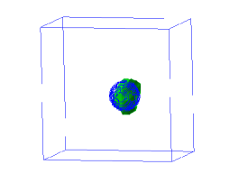
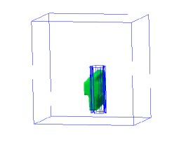
In Tables 2 and 3 we summarize reconstruction results for all objects of Table 1. Table 2 shows shows the reconstructed refractive indices for the non-metallic targets. For these targets, the refractive index n=εr(target)𝑛subscript𝜀rtargetn=\sqrt{\varepsilon_{\mathrm{r}}(\text{target})}. Here, εr(target)subscript𝜀rtarget\varepsilon_{\mathrm{r}}(\text{target}) was chosen as εr(target)=max𝐱Ωεr(𝐱)subscript𝜀rtargetsubscript𝐱Ωsubscript𝜀r𝐱\varepsilon_{\mathrm{r}}(\text{target})=\max_{\mathbf{x}\in\Omega}\varepsilon_{\mathrm{r}}(\mathbf{x}). Table 3 shows the burial depths and the effective dielectric constants of the metallic targets. From Tables 2 and 3 we can see that the burial depth was accurately estimated in most cases, with the errors not exceeding 1 cm.

The estimates of the refractive indices of non-metallic targets with refractive indices larger than that of the sand (water and wet wood) are quite accurate with the average error of about 8.5%.

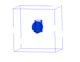
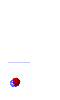
Note that the error in our direct measurement of the refractive index of the wet wood was 10%. For water, we were unable to directly measure its refractive index at the used frequency of the signal, which was about 7.5 GHz. Therefore, we have made a separate experiment described in [22] where we have obtained a reference value n=4.88𝑛4.88n=4.88 for water. We observe from Table 2 that for water we have obtained a value of n𝑛n close to the reference value. Targets with smaller refractive indices than that of the sand are modelling plastic land mines and improvised explosive devices (IEDs). We have observed that in this case we can image these targets only if their burial depths do not exceed 5 cm, see for example, reconstruction of target 3 in Table 2 and in Figure 2-c).

In our experiments we observed that the signals of the metallic targets were stronger compared to the signal from sand. In our previous works, we have established that the effective dielectric constant of metals should be larger than 10–15, see [13, 21]. From Table 3 we see that we have obtained similar results as in our previous studies.

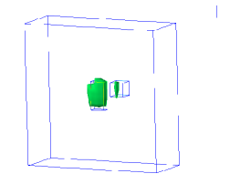
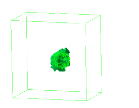
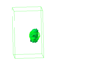
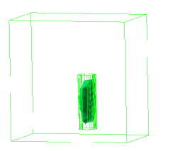
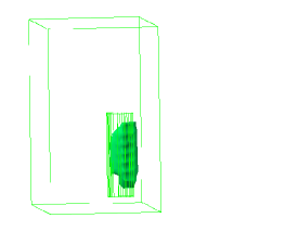
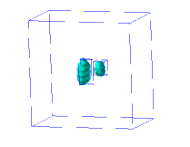
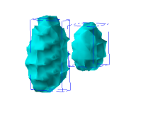
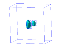
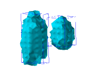
From Table 1 we observe that in our experiments we were supposed to reconstruct two metallic blocks which were placed at 1 cm separation to each other. On the other hand, the wavelength λ𝜆\lambda of our device is 4.5 cm. Thus, λ/4.5𝜆4.5\lambda/4.5 is the distance between these two targets and superresolution is achieved beyond the diffraction limit. Table 3 and Figure 2-d) shows that we have accurately imaged both targets. This phenomenon was not expected and should be studied further because of its importance when combined with quantitative imaging.

7.5 Numerical examples of the second stage

From the results of the first stage we can conclude that this stage provides accurate locations of the targets as well as accurate values of the refractive indices n=εr𝑛subscript𝜀rn=\sqrt{\varepsilon_{\mathrm{r}}} of the dielectric targets and large values of effective dielectric constants εrsubscript𝜀r\varepsilon_{\mathrm{r}} for the metallic targets of interest. However, the approximate globally convergent algorithm does not reconstruct the shapes of the targets in the z𝑧z-direction well, see Figure 2. Because of that we have used the second stage where we have minimized the Tikhonov functional on locally adaptively refined meshes.

7.5.1 Computations of the forward problem

The data g𝑔g in our experiments of the second stage are given only for the second component E2subscript𝐸2E_{2} of the electric field E𝐸E in (12) and are measured at the front side ΓΓ\Gamma of the domain ΩΩ\Omega which is defined as

Γ={𝐱=(x,y,z)Ω:z=0.04}.Γconditional-set𝐱𝑥𝑦𝑧Ω𝑧0.04\Gamma=\{\mathbf{x}=(x,\,y,\,z)\in\partial\Omega:z=0.04\}.

To generate backscattering data for other two components E1subscript𝐸1E_{1} and E3subscript𝐸3E_{3} we solve the forward problem (19)–(24) in the computational domain G𝐺G defined as in the first stage in (45) with the known value of εrsubscript𝜀r\varepsilon_{\mathrm{r}} obtained at the first stage of our two-stage numerical procedure. We use a stabilized domain decomposition method of [9] implemented in the software package WavES [25]. We split G𝐺G into two subdomains ΩFEM=ΩsubscriptΩFEMΩ\Omega_{\mathrm{FEM}}=\Omega and ΩFDMsubscriptΩFDM\Omega_{\mathrm{FDM}} so that G=ΩFEMΩFDM𝐺subscriptΩFEMsubscriptΩFDMG=\Omega_{\mathrm{FEM}}\cup\Omega_{\mathrm{FDM}} and the inner domain is defined as in (46).

Once the forward problem (19)–(24) is solved to generate backscattering data for the two components E1subscript𝐸1E_{1} and E3subscript𝐸3E_{3} at the boundary ΓsuperscriptΓ\Gamma^{\prime}, then after the data immersing procedure described in Section 7.3.3 of [14] the inverse problem is solved via the algorithm of section 6. The immersing procedure of [14] immerses the time-dependent propagated experimental data g(𝐱,t)=E2(𝐱,t)|𝐱Γg\left(\mathbf{x},\,t\right)=E_{2}\left(\mathbf{x},\,t\right)\rvert_{\mathbf{x}\in\Gamma} into the computationally simulated data and then extends the data g𝑔g from ΓΓ\Gamma to ΓsuperscriptΓ\Gamma^{\prime}.

We choose the waveform f𝑓f in (19)–(24) as

f(t)=sin(ωt),0tt:=2πω,formulae-sequence𝑓𝑡𝜔𝑡0𝑡superscript𝑡assign2𝜋𝜔f(t)=\sin(\omega t),\quad 0\leq t\leq t^{\prime}:=\frac{2\pi}{\omega},

where we use ω=30𝜔30\omega=30 and T=1.2.𝑇1.2T=1.2. We solve the problem (19)–(24) using the explicit scheme of [9] with the time step size τ=0.003𝜏0.003\tau=0.003, which satisfies the CFL condition.

7.5.2 Reconstructions

Suppose that in the adaptive algorithm of section 6 we have obtained the function εrsubscript𝜀r\varepsilon_{\mathrm{r}}. We obtain then the image of the dielectric targets based on the function εr,dielsubscript𝜀rdiel\varepsilon_{\mathrm{r,\,diel}} which we define as

εr,diel(𝐱)={εr(𝐱) if εr(𝐱)0.5max𝐱Ω¯εr(𝐱),1 otherwise.subscript𝜀rdiel𝐱casessubscript𝜀r𝐱 if subscript𝜀r𝐱0.5subscript𝐱¯Ωsubscript𝜀r𝐱1 otherwise.\varepsilon_{\mathrm{r,\,diel}}\left(\mathbf{x}\right)=\left\{\begin{array}[]{l}\varepsilon_{\mathrm{r}}\left(\mathbf{x}\right)\text{ if }\varepsilon_{\mathrm{r}}\left(\mathbf{x}\right)\geq 0.5\max_{\mathbf{x}\in\overline{\Omega}}\varepsilon_{\mathrm{r}}\left(\mathbf{x}\right),\\ 1\text{ otherwise.}\end{array}\right.

For metallic targets we used similar function εr,metalsubscript𝜀rmetal\varepsilon_{\mathrm{r,\,metal}},

εr,metal(𝐱)={εr(𝐱) if εr(𝐱)0.5max𝐱Ω¯εr(𝐱),1 otherwise.subscript𝜀rmetal𝐱casessubscript𝜀r𝐱 if subscript𝜀r𝐱0.5subscript𝐱¯Ωsubscript𝜀r𝐱1 otherwise.\varepsilon_{\mathrm{r,\,metal}}\left(\mathbf{x}\right)=\left\{\begin{array}[]{l}\varepsilon_{\mathrm{r}}\left(\mathbf{x}\right)\text{ if }\varepsilon_{\mathrm{r}}\left(\mathbf{x}\right)\geq 0.5\max_{\mathbf{x}\in\overline{\Omega}}\varepsilon_{\mathrm{r}}\left(\mathbf{x}\right),\\ 1\text{ otherwise.}\end{array}\right.

In our experiments we apply the adaptive algorithm of section 6 to improve shape of targets listed in Table 1.

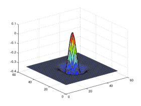
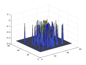
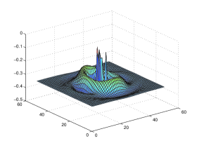
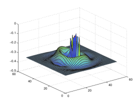
Recall that to apply immersing procedure of the experimental data g𝑔g into simulated data E2subscript𝐸2E_{2} we solve the problem (19)–(24) numerically with the known values of the function εr=εr,globsubscript𝜀rsubscript𝜀rglob\varepsilon_{\mathrm{r}}=\varepsilon_{\mathrm{r,\,glob}} obtained at the first stage of our two-stage numerical procedure, see Tables 2, 3 for the function εr,globsubscript𝜀rglob\varepsilon_{\mathrm{r,\,glob}}. Figure 1 show backscattering immersed data of the second component of electric field E2subscript𝐸2E_{2} for target #4 (two metallic blocks) of Table 1 at different times.

Table 4 lists both computed refractive index ncompsuperscript𝑛compn^{\mathrm{comp}}, obtained via (44), on adaptively refined meshes and directly measured refractive indices n𝑛n of the dielectric targets. Table 5 lists calculated appearing dielectric constants εrcompsuperscriptsubscript𝜀rcomp\varepsilon_{\mathrm{r}}^{\mathrm{comp}} of the metallic targets. From Table 5 we observe that εrcomp>10superscriptsubscript𝜀rcomp10\varepsilon_{\mathrm{r}}^{\mathrm{comp}}>10 for all metallic targets, and thus (42) is satisfied.

An important observation, which can be deduced from Table 5, is that our adaptive algorithm can still compute large inclusion/background contrasts exceeding 10:1.

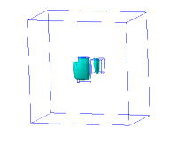
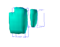
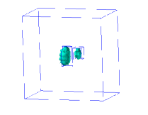
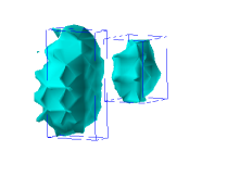
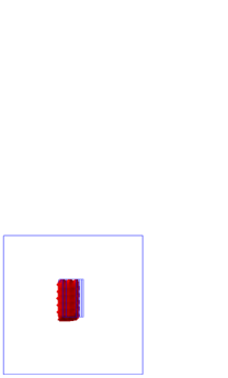
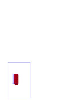
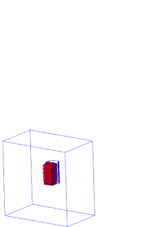
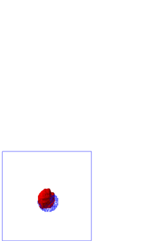
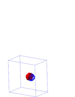
Figures 37 display adaptively refined meshes and 3D images of some targets of Table 1. To have a better visualization, we have zoomed some figures from the domain ΩFEMsubscriptΩFEM\Omega_{\mathrm{FEM}} defined in (46) to the domain defined in (47). We can conclude that the location of all targets as well as their sizes in the x𝑥x-, y𝑦y-, and z𝑧z-directions are well estimated on the second stage of our two-stage numerical procedure.

Object Blind/ Description of target Material
# Non-blind
1 Non-blind A metallic ball, 3 cm burial depth Metal
2 Non-blind A bottle filled with clear water, 3 cm depth Water
3 Blind A ceramic mug, 5 cm burial depth Ceramic
4 Non-blind Two metallic blocks at 1 cm separation Metal/Metal
Table 1: Description of the data sets.
Object Material Computed Exact Computed Measured
# depth depth n𝑛n n𝑛n
2 Water 3.6 4.0 4.7 4.88
3 Ceramic 4.0 5.0 1.0 1.39
Table 2: Result of the first stage: the refractive indices n=εr𝑛subscript𝜀rn=\sqrt{\varepsilon_{\mathrm{r}}} and the burial depths of non-metallic targets.
Object Material Computed Exact Computed εrsubscript𝜀r\varepsilon_{\mathrm{r}}
# depth depth
1 Metal 2.9 3.0 31.0
4 Metal 3.8 4.0 99.8
Metal 4.0 4.0 56.5
Table 3: Result of the first stage: the estimated effective dielectric constants and the burial depths of metallic targets. Object #4 consists of two metallic targets with 1 cm distance between their surfaces.
Target number 2 3
blind (yes/no) no no
Measured n𝑛n 4.88 1.39
ncompsuperscript𝑛compn^{\mathrm{comp}} coarse mesh 4.7 1
ncompsuperscript𝑛compn^{\mathrm{comp}} 1 time ref. mesh 4.7 1
ncompsuperscript𝑛compn^{\mathrm{comp}} 2 times ref.mesh 4.7 1
ncompsuperscript𝑛compn^{\mathrm{comp}} 3 times ref.mesh 4.7 1
Table 4: Stage 2. Computed ncompsuperscript𝑛compn^{\mathrm{comp}} and directly measured n𝑛n refractive indices of dielectric targets.
Target number 1 4
blind (yes/no) no no
εrcompsuperscriptsubscript𝜀rcomp\varepsilon_{\mathrm{r}}^{\mathrm{comp}} coarse mesh 24.5 75.6
εrcompsuperscriptsubscript𝜀rcomp\varepsilon_{\mathrm{r}}^{\mathrm{comp}} 1 time ref. mesh 24.6 100
εrcompsuperscriptsubscript𝜀rcomp\varepsilon_{\mathrm{r}}^{\mathrm{comp}} 2 times ref.mesh 24.7 100
εrcompsuperscriptsubscript𝜀rcomp\varepsilon_{\mathrm{r}}^{\mathrm{comp}} 3 times ref.mesh 24.6 100
Table 5: Stage 2. Computed appearing dielectric constants εrcompsuperscriptsubscript𝜀rcomp\varepsilon_{\mathrm{r}}^{\mathrm{comp}} of metallic targets.
Refer to caption Refer to caption
a) t=0.3 b) t=0.3
Refer to caption Refer to caption
c) t=0.45 d) t=0.45
Figure 1: Backscattering immersed data of the second component E2subscript𝐸2E_{2} of the electric field for object 4 (two metallic blocks at 1 cm separation) of Table 1. On the left we show backscattering immersed data which are immersed into measured data without presence of sand, on the right - with presence of sand. Recall that the final time is T=1.2𝑇1.2T=1.2.
Refer to caption Refer to caption
a) target 1 b) target 2
Refer to caption Refer to caption
c) target 3 d) targets 4
Figure 2: Reconstructions of targets of Table 1 obtained on the first stage of our two-stage numerical procedure.
Refer to caption Refer to caption
a) three times refined mesh, xy𝑥𝑦xy-view b) three times refined mesh, yz𝑦𝑧yz-view
Figure 3: Computed image of target number 1 of Table 1 . Thin lines indicate correct shape. To have a better visualization we have zoomed the domain ΩΩ\Omega in (46) in the domain ΩFEMsubscriptΩFEM\Omega_{\mathrm{FEM}} in (47).
Refer to caption Refer to caption
a) twice refined mesh, xy𝑥𝑦xy-view b) twice refined mesh, yz𝑦𝑧yz-view
Figure 4: Computed image of target number 2 of Table 1 . Thin lines indicate correct shape. To have a better visualization we have zoomed the domain ΩΩ\Omega in (46) in the domain ΩFEMsubscriptΩFEM\Omega_{\mathrm{FEM}} in (47). This target, which was a plastic bottle filled with water, was quite a large vertical size of 20 cm. On the other hand, our incident signal had a low power, which was much lower at the top and bottom of this target. This is why we were unable to image well the vertical size of this target. Still, one can observe that the image is stretched in the vertical direction.
Refer to caption Refer to caption
a) coarse mesh b) zoomed view
Refer to caption Refer to caption
c) two times refined mesh d) zoomed view
Refer to caption Refer to caption
e) three times refined mesh f) zoomed view
Refer to caption Refer to caption
g) four times refined mesh h) zoomed view
Figure 5: Computed images of targets number 4 of Table 1 when superresolution is achieved on four times adaptively refined meshes. Compare with Figure 2-d).
Refer to caption Refer to caption Refer to caption
(a) Front (b) Side (c) Perspective
Refer to caption Refer to caption Refer to caption
(d) Front, zoomed (e) Side, zoomed (f) Perspective, zoomed
Figure 6: Three views and zooms of the reconstruction of the target number 3 of Table 1 on the once refined mesh. Recall that target number 3 is a ceramic mug.
Refer to caption Refer to caption Refer to caption
(a) Front (b) Side (c) Perspective
Refer to caption Refer to caption Refer to caption
(d) Front, zoomed (e) Side, zoomed (f) Perspective, zoomed
Figure 7: Three views and zooms of the reconstruction of the target number 1 of Table 1 on the three times refined mesh. The initial guess in this test is taken from Test 2 of [22], see Figure 5.1-b),d) of [22]. Recall that target number 1 is a metallic ball.

8 Summary

This is the fifth (5th) paper (after [13, 14, 21, 22]) in the recent series of publications of this group about the performance of the two-stage numerical procedure of [12] on experimental backscattering time-dependent data generated by a single location of the source of electromagnetic waves. While in [13, 14, 21] we have considered the case of targets placed in air, in [22] and here we consider the more challenging case of targets buried in the ground. This case is more challenging because the signal scattered by the ground is heavily mixed with the signal scattered by the target.

It was shown in [22] that the globally convergent numerical method of [12] accurately images refractive indices and locations of buried targets. In this paper we complement the globally convergent method by the locally convergent adaptivity technique. The adaptivity takes the image of the globally convergent method as the starting point for subsequent iterations. The theory of the adaptivity can be found in [2, 3, 4, 5, 6, 7, 8], [10, 11, 12], and [26]. In particular, the important analytical guarantee of the fact that adaptivity indeed refines images was first established in [6] and then also published in [12] and [26].

As a result of the application of the adaptivity, our images are significantly refined: the shapes of the targets are accurately imaged. A particularly interesting case is the case of the superresolution (Figure 2-d and Figures 5). We have accurately imaged both targets in this case.

In conclusion, we believe that the two-stage numerical procedure of [12] is now completely verified on experimental data.

Acknowledgments

This research was supported by US Army Research Laboratory and US Army Research Office grant W911NF-11-1-0399, the Swedish Research Council, the Swedish Foundation for Strategic Research (SSF) through the Gothenburg Mathematical Modelling Centre (GMMC). The computations were performed on resources at Chalmers Centre for Computational Science and Engineering (C3SE) provided by the Swedish National Infrastructure for Computing (SNIC).

References

  • [1] H. Ammari, J. Garnier, J. de Rosny, Knut Solna, Medium induced resolution enhancement broadband imaging, Inverse problems, 30, 085006, 2014.
  • [2] M.Asadzadeh, L.Beilina, A posteriori error analysis in a globally convergent numerical method for a hyperbolic coefficient inverse problem, Inverse Problems, 26, 115007, 2010.
  • [3] M.V. Klibanov, A.B. Bakushinskii and L. Beilina, Why a minimizer of the Tikhonov functional is closer to the exact solution than the first guess? J. Inverse and Ill-posed problems, 19, 83-105, 2011
  • [4] L. Beilina and M.V. Klibanov, Synthesis of global convergence and adaptivity for a hyperbolic coefficient inverse problem in 3D, J. Inverse and Ill-posed Problems, 18, 85-132, 2010.
  • [5] L. Beilina and M.V. Klibanov, A posteriori error estimates for the adaptivity technique for the Tikhonov functional and global convergence for a coefficient inverse problem, Inverse Problems, 26, 045012, 2010.
  • [6] L. Beilina, M.V. Klibanov and M.Yu. Kokurin, Adaptivity with relaxation for ill-posed problems and global convergence for a coefficient inverse problem, Journal of Mathematical Sciences, 167, 279-325, 2010.
  • [7] L. Beilina and C. Johnson, A hybrid FEM/FDM method for an inverse scattering problem. In Numerical Mathematics and Advanced Applications, ENUMATH 2001, Springer-Verlag, Berlin, 2001.
  • [8] Beilina, Adaptive hybrid FEM/FDM methods for inverse scattering problems, Inverse problems and information technologies, 1 (3), 73-116, 2002
  • [9] L. Beilina, Energy estimates and numerical verification of the stabilized domain decomposition finite element/finite difference approach for the Maxwell’s system in time domain, Central European Journal of Mathematics, 11, 702-733, 2013.
  • [10] L. Beilina, Adaptive Finite Element Method for a coefficient inverse problem for the Maxwell’s system, Applicable Analysis, 90 (10), 1461-1479, 2011.
  • [11] L. Beilina and C. Johnson, A posteriori error estimation in computational inverse scattering, Mathematical Models in Applied Sciences, 1, 23-35, 2005.
  • [12] L. Beilina and M.V. Klibanov, Approximate Global Convergence and Adaptivity for Coefficient Inverse Problems, Springer, New York, 2012.
  • [13] L. Beilina, Nguyen Trung Thành, M. V. Klibanov, M. A. Fiddy, Reconstruction from blind experimental data for an inverse problem for a hyperbolic equation, Inverse Problems 30, 025002, doi:10.1088/0266-5611/30/2/025002, 2014
  • [14] L. Beilina, Nguyen Trung Thành, M. V. Klibanov, J.Bondestam Malmberg, Reconstruction of shapes and refractive indices from backscattering experimental data using the adaptivity, to appear in Inverse Problems. Preprint, available online at Chalmers Publication Library, http://www.math.chalmers.se/Math/Research/Preprints/, preprint number 2014-9.
  • [15] S. C. Brenner and L. R. Scott, The Mathematical theory of finite element methods, Springer-Verlag, Berlin, 1994.
  • [16] A.L. Bukhgeim and M.V. Klibanov, Uniqueness in the large of a class of multidimensional inverse problems, Soviet Math. Doklady, 17, 244-247, 1981.
  • [17] F.-C. Chen and W. C. Chew, Experimental verification of superresolution in nonlinear inverse scattering, App. Phys. Lett., 72, issue 23, 3081-3086, 1998.
  • [18] B. Engquist and A. Majda, Absorbing boundary conditions for the numerical simulation of waves,  Math. Comp., 31, 629-651, 1977.
  • [19] K. Eriksson, D. Estep and C. Johnson, Calculus in Several Dimensions, Springer, Berlin, 2004.
  • [20] A.V. Kuzhuget, L. Beilina, M.V. Klibanov, A. Sullivan, L. Nguyen and M.A. Fiddy, Blind experimental data collected in the field and an approximately globally convergent inverse algorithm, Inverse Problems, 28, 095007, 2012.
  • [21] Nguyen Trung Thành, L. Beilina, M. V. Klibanov and M. A. Fiddy, Reconstruction of the refractive index from experimental backscattering data using a globally convergent inverse method, SIAM J. Scientific Computing, 36, B273-B293, 2014.
  • [22] Nguyen Trung Thành, L. Beilina, M. V. Klibanov and M. A. Fiddy, Imaging of buried objects from experimental backscattering radar measurements using a globally convergent inverse algorithm, Preprint, available online at Chalmers Publication Library, http://www.math.chalmers.se/Math/Research/Preprints/, preprint number 2014-15.
  • [23] O.Pironneau, Optimal shape design for elliptic systems, Springer-Verlag, Berlin, 1984.
  • [24] F. Simonetti. Localization of pointlike scatterers in solids with subwavelength resolution. Applied Physics Letter, 89:094105, 2006.
  • [25] WavES, the software package, http://www.waves24.com
  • [26] L. Beilina and M.V. Klibanov, Relaxation property for the adaptivity for ill-posed problems, Applicable Analysis, 93(2), 223-253, 2013.