Abstract

We apply a modified proper orthogonal decomposition (POD) to large eddy simulation data of a wind turbine wake in a turbulent atmospheric boundary layer. The turbine is modeled as an actuator disk. Our analysis mainly focuses on the pragmatic identification of spatial modes, which yields a low order description of the wake flow. This reduction to a few degrees of freedom is a crucial first step for the development of simplified dynamic wake models based on modal decompositions. It is shown that only a few modes are necessary to capture the basic dynamical aspects of quantities that are relevant to a turbine in the wake flow. Furthermore, we show that the importance of the individual modes depends on the relevant quantity chosen. Therefore, the optimal choice of modes for a possible model could in principle depend on the application of interest. We additionally present a possible interpretation of the extracted modes by relating them to the specific properties of the wake. For example, the first mode is related to the horizontal large-scale movement.

10.3390/—— 8 Received: 21 August 2014 / Accepted: 20 January 2015 / Published: 2015 Towards a Simplified Dynamic Wake Model Using POD Analysis David Bastine *, Björn Witha, Matthias Wächter and Joachim Peinke E-Mail: david.bastine@uni-oldenburg.de; Tel.: +49-441-798-5054.
Academic Editor: Frede Blaabjerg

1 Introduction

Due to economical and technological benefits, wind turbines are often arranged in clusters that can contain up to hundreds of turbines. One of the key issues of these wind farms is the wake effect. A wind turbine in the wake of another turbine experiences a strongly altered inflow, resulting in reduced power production and higher dynamic loads acting on the turbine. In order to minimize these effects, a detailed understanding and efficient modeling of wakes is essential. This is of particular importance in the planning phase of a farm, where an optimized layout can result in a much higher energy production Barthelmie et al. (2010) and longer lifetimes of the turbines. Furthermore, good wake models are an important tool for an efficient wind farm control Goit and Meyers (2014); Storey et al. (2014). It has, for example, been shown that wake deflection through yawing of the turbines can mitigate the wake effect Medici (2005); Jimenez et al. (2010); Fleming et al. (2014).

The hydrodynamic equations describing the dynamics of a wind turbine wake and the flow through a wind farm are well known. However, solving these equations in acceptable time is currently impossible due to the many scales involved in turbulent flows. A very successful modeling tool for turbulent flows is large eddy simulation (LES), which solves the hydrodynamic equations on the large scales of the flow, but models the influence of the smaller scales by sub-grid-scale turbulence models (e.g., Pope (2000)). Combined with simplified turbine models, such as actuator disk and actuator line, LESs have been increasingly applied in wind energy research Jimenez et al. (2007); Calaf et al. (2010); Porté-Agel et al. (2011); Goit and Meyers (2014); Storey et al. (2014); Witha et al. (2014). Unfortunately, they are still too time consuming for many practical applications, such as the optimization of a wind farm layout or wind farm control.

Therefore, steady-state wake models, such as Jensen (1983); Ainslie (1988); Larsen (1988); Frandsen (2003); Frandsen et al. (2006), are still the state-of-the-art for many purposes. These models can, for example, use empirical descriptions of the velocity deficit, such as Jensen (1983), or mean field solutions to strongly approximated versions of the fluid dynamical equations, such as Ainslie (1988). More recently, mean field wakes stemming from computational fluid dynamic simulations have been used in the context of layout optimization with respect to power Schmidt (2014). Instead of modeling the velocity deficit itself, Frandsen Frandsen (2003) uses an effective turbulence intensity to model the fatigue loads in a wind park. However, all of the models neglect the dynamical aspects of the wake, which are commonly expected to be relevant for the loads and power production of a turbine in a wake.

The first step to incorporate the dynamical aspects of the wake is to take the meandering movement of the velocity deficit into account. Usually, this is done under the assumption that the meandering is mainly caused by the large-scale dynamics of the atmospheric boundary layer (ABL) Larsen et al. (2007, 2008); Trujillo et al. (2011); España et al. (2012). While this is a very promising approach Thomsen and Madsen (2005); Thomsen et al. (2007), these models neglect, for example, the dynamically changing shape of the velocity deficit, which is also expected to be relevant, particularly for the loads on the turbine. Moreover, it is not fully clear whether the passive tracer assumption always yields a good description of the meandering Andersen et al. (2013). Thus, there is still a need for improved simplified dynamic wake models that yield a good description of the inflow conditions of a wind turbine, but avoid too complex numerical simulations.

An alternative approach to simplified modeling, used in fluid dynamics, is to decompose the flow into a superposition of spatial modes Berkooz et al. (1993); Citriniti and George (2000); Jung et al. (2004); Iqbal and Thomas (2007); Tutkun et al. (2008) and to develop reduced order models for specific flow problems Berkooz et al. (1993); Delville et al. (1999); Bergmann et al. (2005); Cordier et al. (2013). Andersen et al. Andersen et al. (2014, 2013) applied the proper orthogonal decomposition (POD) to LES data of a wake in an infinitely long row of turbines modeled with an actuator line approach. They found clearly structured POD modes, which could be a first step toward a reduced order model of wakes in a long row of turbines. Additionally, their results indicate that the low-frequency dynamics of the wake are not only caused by the large-scale dynamics of the ABL and can, thus, not be treated separately from the wake itself.

This work is also motivated by the idea of reduced order modeling based on modal decompositions of the wake flow. Such reduced models could play an important role in the layout optimization and controlling of wind farms. They could therefore provide a useful alternative to the kinematic approach followed in dynamic wake meandering models Larsen et al. (2007, 2008). The main goal of this paper is to identify spatial modes that yield a low dimensional description of the velocity field, while still preserving important aspects of the wake, relevant to a sequential turbine. A strong dimensional reduction of the flow is a crucial step for the development of low order models, since it facilitates the application of the huge toolbox of advanced modeling methods of nonlinear dynamical systems Kantz and Schreiber (2004); Argyris et al. (2010); Kleinhans and Friedrich (2007); Friedrich et al. (2011); Milan et al. (2014).

For this purpose, we apply the POD to LES data of a wind turbine wake. In contrast to Andersen et al. Andersen et al. (2014, 2013), we analyze the wake of a single turbine modeled by an actuator disk and use a turbulent ABL as the inflow condition. Additionally, we apply threshold criteria to focus on the wake structure. After this preprocessing procedure, we estimate POD modes and use them to reconstruct the original wake flow. We propose to assess the quality of such reconstructions based on the potential impact on a turbine in the wake instead of using the turbulent kinetic energy. The results in Bastine et al. (2014) gave the first hint that relevant quantities of the wake can be described well, even though only a small part of the turbulent kinetic energy is recovered. Here, we investigate three additional quantities, which are related to the power, thrust and yaw load on a virtual turbine in the wake and perform a detailed comparison. This comparison naturally leads to the idea of selecting modes depending on the desired application of a possible model. A similar approach has also been suggested by Saranyasoontorn and Manuel Saranyasoontorn and Manuel (2005, 2006) in the case of an ABL inflow. Furthermore, we interpret the role of the different modes. This enables us to relate our reduced order modeling approach to features of other dynamic wake models.

In Section 2 of this work, we describe the LES data used for our analysis. Section 3.1 introduces the concept of modal decompositions and motivates our main goal of dimensional reduction in a more formal way. This is followed by a brief description of the POD theory (Section 3.2). Section 3.3 describes the preprocessing, which we apply before estimating the corresponding POD modes in Section 3.4. Next, we use the extracted modes to investigate approximations of the original velocity field depending on the number of modes used for reconstruction (Section 3.5). In Section 4, we introduce the general concept of assessing the quality of POD reconstructions through measures related to a turbine in the wake flow. We define four simple measures (e.g., the energy flux through a disk) and compare the corresponding results in Section 4.3. In Section 5, we further investigate the role of the individual POD modes and try to relate them to the specific properties of the wake. Finally, the conclusions drawn from our results are presented in Section 6.

2 LES Data

The LES data that will be analyzed in this work have been generated by performing simulations with the parallelized LES Model PALM Raasch and Schröter (2001); Maronga et al. (2014), which has been widely used for studies of the atmospheric boundary layer. PALM solves the filtered, incompressible, non-hydrostatic Navier–Stokes equations under the Boussinesq approximation. The sub-grid-scale turbulence parameterization is based on the 1.5-order scheme of Deardorff Deardorff (1980). The lateral boundary conditions are periodic, and no-slip conditions are used at the lower boundary. At the top of the domain, a Dirichlet boundary condition with a constant geostrophic wind of $u_{g}$ = $10$ ms^-1 is used. For further details on the PALM model, we refer the reader to Raasch and Schröter (2001).

The wind turbine is modeled by a standard, uniformly-loaded actuator disk. This approach yields very similar far wake characteristics as more complex turbine parameterizations, such as the actuator line method Witha et al. (2014); Wu and Porté-Agel (2011). The simulated wind turbine has a rotor diameter of $D=100$ m and a hub height of $160$ m. A constant thrust coefficient of $C_{T}=0.75$ was applied.

A stationary and fully-turbulent neutral ABL is generated in a precursor simulation without the wind turbine using periodic inflow conditions. An aerodynamic roughness length of $z_{0}$ = $0.05$ m is prescribed. The Coriolis force is neglected, so that the mean flow is aligned with the x-axis in all heights. After 12 h, a stationary inflow is achieved. In the main simulation with the wind turbine, non-cyclic inflow conditions are applied. The final horizontally and time-averaged velocity and temperature profiles of the precursor simulation are used as the fixed inflow profile. Furthermore, the instantaneous fields of the precursor simulation are periodically mapped onto the domain of the main simulation. The turbulence is continuously recycled at every time step by picking up the turbulent fluctuations in a yz-plane downstream of the inflow and imposing them onto the fixed mean inflow profile. The distance between this yz-plane and the inflow boundary is chosen large enough that all turbulent scales are preserved. More details on this recycling method can be found in Witha et al. (2014); Kataoka and Mizuno (2002). A notable property of this ABL flow is the existence of large-scale coherent regions of high or low velocity. These regions have the form of stripes aligned with the stream-wise velocity direction and originate from the surface layer. They are a known phenomenon, called streaks, and occur in neutral and stable atmospheres (see, e.g., Witha et al. (2014); Moeng and Sullivan (1994)). We expect the low and high velocity regions in the mean field of the flow without turbine (Figure 1(a)) to be a fingerprint of such structures.

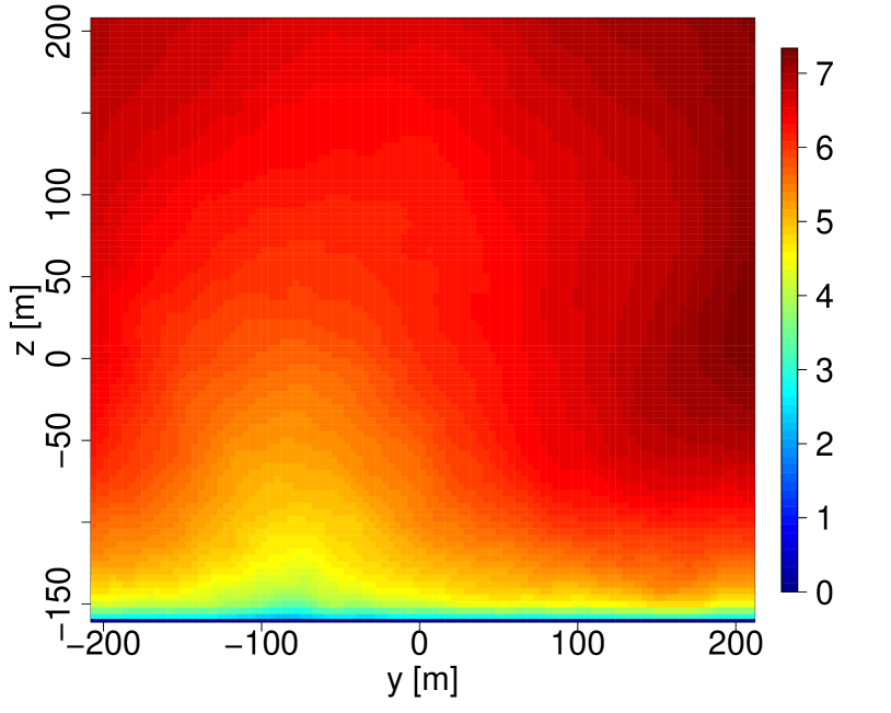
(a)

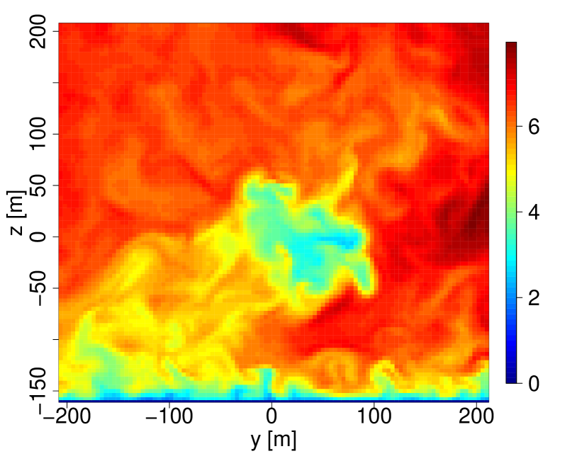
(b)

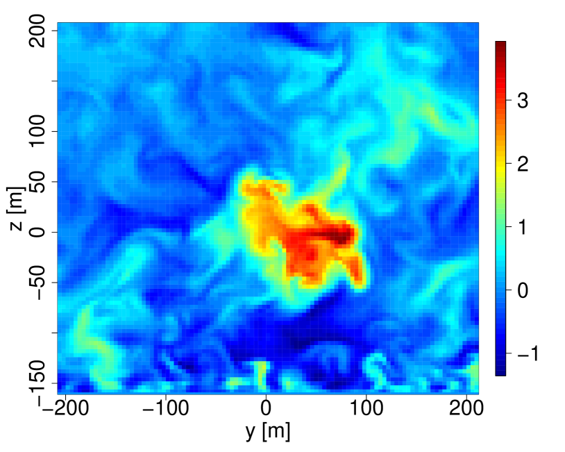
(c)

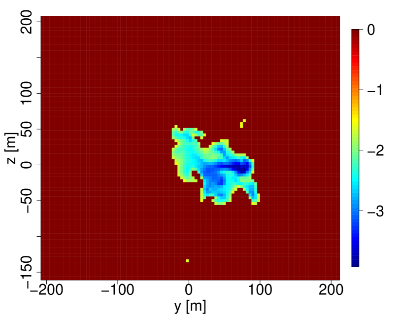
(d)

Figure 1: (a) Time-averaged velocity field without turbine; (b) wake $u(y,z)$ at distance $x=4D$ and $t=500$ s; (c) wake after subtracting the time-averaged velocity field without the turbine; (d) wake after applying the threshold.

The domain size of the main simulation is about $8$ km $\times$ $2$ km $\times$ $0.5$ km with a grid size of $4$ m. With this large domain, we ensure that the wake is virtually unaffected by the boundaries. As shown in Figure 2, we define the $x$-direction aligned with the main flow, $y$ as the lateral and $z$ as the vertical coordinate. The turbine is placed in the center of the domain in $y$-direction and 2500 m downstream of the inflow. Hereafter, the origin of the coordinate system will be located at the hub of the turbine.

The generated data are written out at a rate of $2$ Hz with a time series length of 11,750 s after excluding the first $500$ s of the simulation. For our analysis, we focus on data in a $yz$-plane perpendicular to the main flow, which is placed $4D$ downstream of the turbine (the white dashed line in Figure 2(a)). At this distance, we expect only minor differences between the standard actuator disk model used here and more sophisticated actuator models Wu and Porté-Agel (2011); Witha et al. (2014). Furthermore, we confine our analysis to the main velocity component yielding a spatio-temporal data field $u(y,z,t)$. A snapshot of this data field for $t=500$ s can be seen in Figure 2(b). It shows a pronounced wake downstream of the turbine with a strong reduction of the flow velocity.

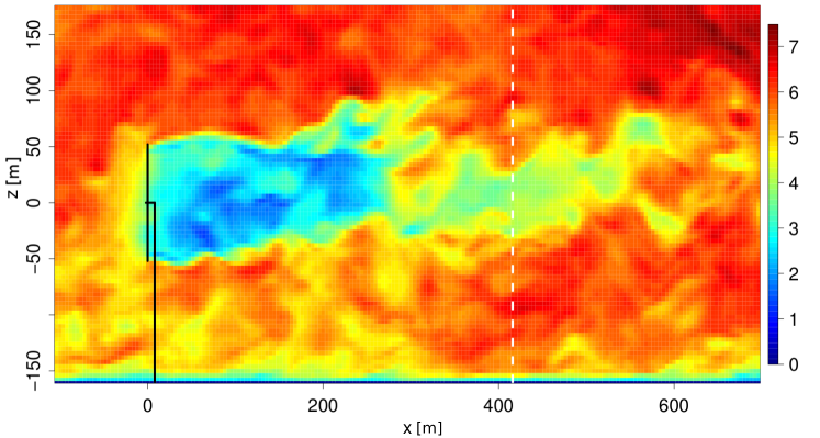
(a)

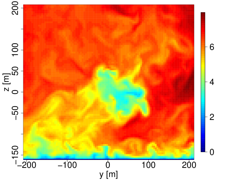
(b)

Figure 2: Snapshots of the analyzed LES data. (a) $xz$-plane ($y=0$ m); (b) $yz$-plane ($x~{}=~{}4~{}D$). The color contours denote the main velocity component $u$ in ms^-1. The white dashed line marks the $yz$-plane at $x=4D$, which was used for the POD analysis.

3 Decomposing the Velocity Field

3.1 Modal Decompositions and Reduced Order Modeling

To develop a simplified dynamic wake model based on a modal decomposition, two essential steps are necessary. The first step is to find a reduced order description of the flow given by a superposition of spatial modes $\phi_{j}(y,z)$. Thus, we define:

$$u^{(N)}(y,z,t)=\langle u(y,z,t)\rangle_{t}+\sum\limits_{j=1}^{N}{a}_{j}(t){\phi}_{j}(y,z)~{}$$ (1)

where $\langle...\rangle_{t}$ denotes the time average and $N$ the order of the reduced description $u^{(N)}$ in terms of the number of modes taken into account. For orthogonal modes, as used in this work, the $a_{j}(t)$ are given through:

$$a_{j}(t)=(\phi_{j}|u^{\prime}):=\int\limits dydz~{}\phi_{j}^{*}(y,z)u^{\prime}(y,z,t)~{}$$ (2)

where $u^{\prime}(y,z,t):=u(y,z,t)-\langle u(y,z,t)\rangle_{t}$ denotes the fluctuating part of the field.

The second step to develop a dynamic wake model is to model the time-dependent weighting coefficients $a_{j}(t)$. Such a model could then be given by an $N$-dimensional dynamical system in the form of:

$$\dot{a}_{j}=f_{j}(a_{1},..a_{N})~{},\mbox{with}~{}j=1,...,N~{}$$ (3)

For this temporal modeling, the order $N$ of the reduced system Equation (3) is crucial. In the case of large $N$, estimating such models from data becomes principally very difficult, and often, huge amounts of data are needed. If $N$ is chosen too small, important information of the velocity field is lost. Thus, the success of the temporal modeling of the $a_{j}(t)$ strongly depends on the reduced order description chosen in the first step. Hence, we aim for identifying modes that yield the necessary dimensional reduction, while preserving important aspects of the flow.

A useful tool to obtain spatial modes and a corresponding decomposition in the spirit of Equation (1) is the POD, which is described in the next section (Section 3.2). In this work, we will not focus on the standard POD modes of the velocity field $u$, but choose the $\phi_{j}$ in a slightly different manner, as will be explained in Section 3.3.

3.2 POD Theory

Subsequently, we briefly illustrate the mathematical definition and important properties of the POD. Details can be found, e.g., in Berkooz et al. (1993).

As its name suggests, the proper orthogonal decomposition (POD) is a decomposition in the spirit of Equation (1). The modes $\phi_{j}$ are then called POD modes and are the optimal modes with respect to the turbulent kinetic energy of the flow. More exactly, they are defined as the orthogonal functions that minimize the mean squared error:

$$\langle\|u^{\prime}(y,z,t)-\sum\limits_{j=1}^{N}a_{j}(t)\phi_{j}(y,z)\|_{2}^{2}\rangle_{t}~{},~{}\mbox{with}~{}a_{j}(t)=(\phi_{j}|u^{\prime})~{}$$ (4)

Note that, in our case and in the rest of this work, only the stream-wise turbulent kinetic energy is taken into account.

Using a variational approach, one can show that the described minimization problem is equivalent to the eigenvalue equation of the covariance operator.

$$\int\limits dy^{\prime}dz^{\prime}~{}\langle u^{\prime}(y,z,t)u^{\prime*}(y^{\prime},z^{\prime},t)\rangle_{t}~{}\phi_{j}(y^{\prime},z^{\prime})=\lambda_{j}\phi_{j}(y,z)~{}\mbox{with}~{}\lambda_{1}>\lambda_{2}>...$$ (5)

This equivalence is the main reason why the POD is a simple, but powerful tool. Instead of treating a complex optimization problem, we can now simply solve an eigenvalue problem of an Hermitian operator. In practice, Equation (5) is often approximated by the eigenvalue problem of the discretized covariance matrix $C_{ij}=\langle u_{i}(t)u_{j}^{*}(t)\rangle_{t}$, where $u_{k}$ is the value of $u$ at the k-th grid point.

We can conclude from the Hilbert–Schmidt theory that the modes are orthogonal with $(\phi_{i}|\phi_{j})=\delta_{ij}$ and that the covariance operator is diagonal in the POD basis, yielding a linearly decorrelated description:

$$\langle a_{i}(t)^{*}a_{j}(t)\rangle_{t}=\lambda_{i}\delta_{ij}~{}$$ (6)

Due to Parseval’s relation:

$$\langle\|u^{\prime}(y,z,t)\|^{2}_{2}\rangle_{t}:=\langle\int\limits dydz~{}|u^{\prime}(y,z,t)|^{2}\rangle_{t}=\sum\limits_{j=1}^{\infty}\langle|a_{j}|^{2}\rangle_{t}~{}~{}\mbox{and}~{}~{}\langle|a_{j}(t)|^{2}\rangle_{t}=\lambda_{j}~{}$$ (7)

the $\mbox{j}^{\mbox{th}}$ eigenvalue can be interpreted as a measure for the kinetic energy contained in the $\mbox{j}^{\mbox{th}}$ mode yielding for the mean squared error of a reconstruction:

$$\langle\|u^{\prime}-{u^{\prime}}^{(N)}\|_{2}^{2}\rangle_{t}=\sum\limits_{j=N+1}^{\infty}\lambda_{j}=\langle\|u^{\prime}\|_{2}^{2}-\|{u^{\prime}}^{(N)}\|_{2}^{2}\rangle_{t}~{}$$ (8)

where ${u^{\prime}}^{(N)}=\sum\limits_{j=1}^{N}a_{j}(t)\phi_{j}(y,z)$. For many applications, the method of snapshots (see, e.g., Berkooz et al. (1993)) is used instead of directly solving Equation (5). Here, we solve the direct problem, since the number of time steps used for the analysis is of the same order as the number of grid points. Therefore, the method of snapshots is not more efficient.

We could now apply the POD method to the data field $u(y,z,t)$. The results based on this standard decomposition are discussed in Appendix A. In the next section, we introduce a slightly different approach, which is used throughout the rest of this work.

3.3 Preprocessing and Modified Decomposition

In this work, we aim to describe the wake in the turbulent ABL without describing the dynamics of the ABL itself. Thus, in the following, we introduce two preprocessing steps that separate the wake structure from the ABL flow. Note that despite this separation, the extracted wake structure still contains information about the response of the wake to the ABL dynamics.

As the first preprocessing step, the time-averaged velocity field of the flow without turbine (Figure 1(a)) is subtracted from $u(y,z,t)$. This leads to a slightly better separation from the ABL structures (Figure 1(c)). Second, we extract the deficit by using a (temporally local) relative threshold. This means that we set all values smaller than 40% of the current deficit maximum to zero (Figure 1(d)). A similar procedure has also been applied in España et al. (2011). The results presented in the following are relatively robust against the choice of the threshold. Similar results are obtained for choosing 20%–50%. In the following, the preprocessed field will be called $\tilde{u}(y,z,t)$, with the corresponding POD modes $\tilde{\phi_{j}}$.

In Section 3.5, we apply the obtained modes $\tilde{\phi_{j}}$ to reconstruct the original velocity field $u(y,z,t)$ (not $\tilde{u}$). Thus, Equation (1) becomes:

$$u^{(N)}(y,z,t):=\langle u(y,z,t)\rangle_{t}+\sum\limits_{j=1}^{N}{a}_{j}(t)\tilde{\phi}_{j}(y,z)~{},~{}\mbox{with}~{}{a}_{j}:=(\tilde{\phi}_{j}|u^{\prime})~{}$$ (9)

This way, we do not investigate a standard proper orthogonal decomposition of $u$, but a modified decomposition of $u$ using the POD modes of the preprocessed field $\tilde{u}$. In Appendix A, we briefly point out the advantages of this alternative approach, which probably stem from the fact that the modes $\tilde{\phi_{j}}$ focus solely on the wake structure. To model the complete inflow of a turbine in the wake, a model, such as Mann (1998), could be added to model the ambient field.

It is important to note that similar results as presented in this work can be obtained when using $\tilde{\phi}_{j}$ for a reconstruction of the corresponding preprocessed field $\tilde{u}$.

3.4 POD Modes of the Preprocessed Field

Next, we calculate the covariance matrix corresponding to the preprocessed field $\tilde{u}$ and numerically solve its eigenvalue problem analogous to Equation (5). The obtained eigenvectors are the POD modes $\tilde{\phi}_{j}$, which are shown in Figure 3. The modes show clear structures with a trend from larger to smaller scales with increasing mode number. This trend is easily explained by the fact that the modes are sorted with respect to energy and that the kinetic energy in a turbulent flow typically decreases with scale.

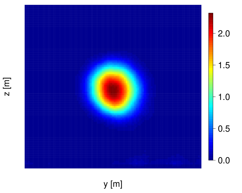
(a)

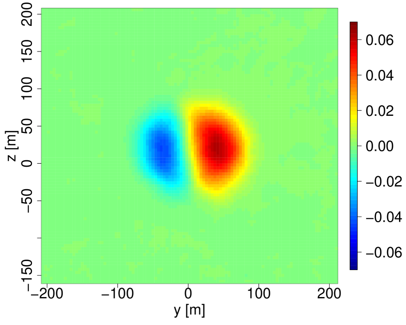
(b)

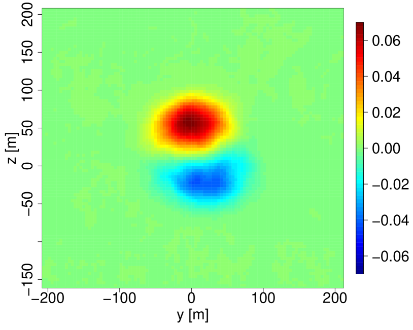
(c)

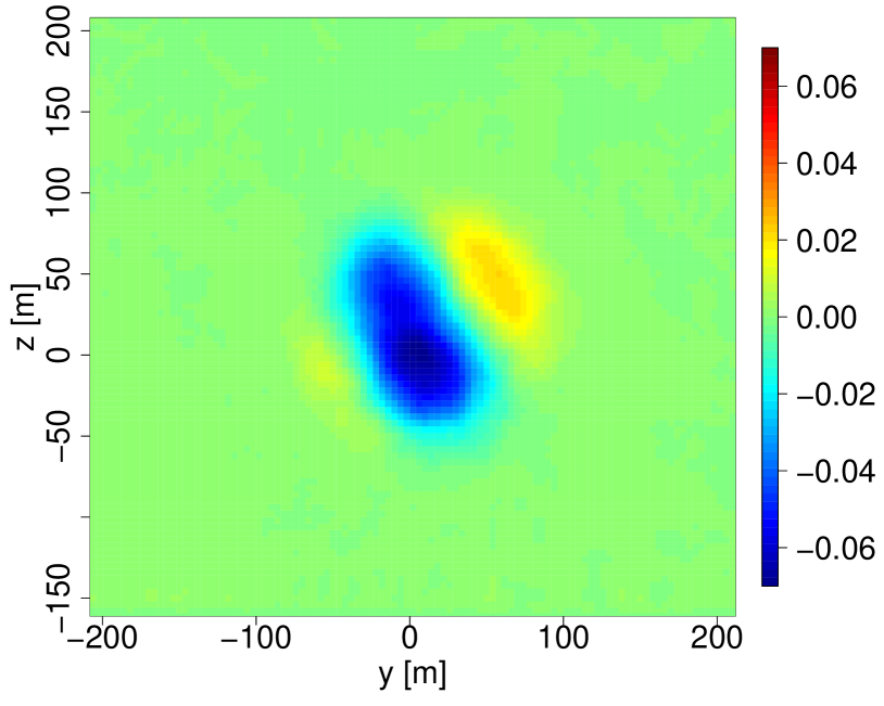
(d)

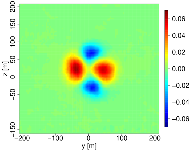
(e)

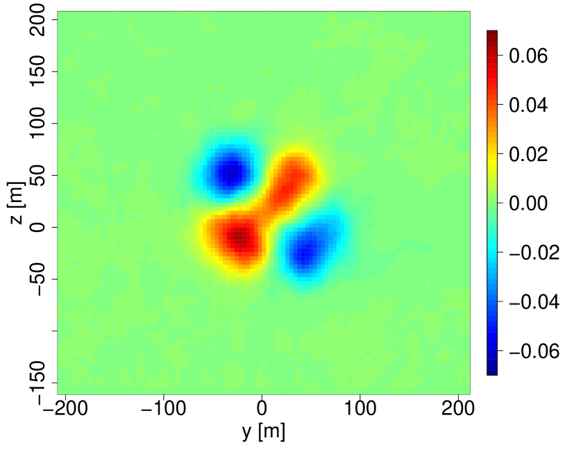
(f)

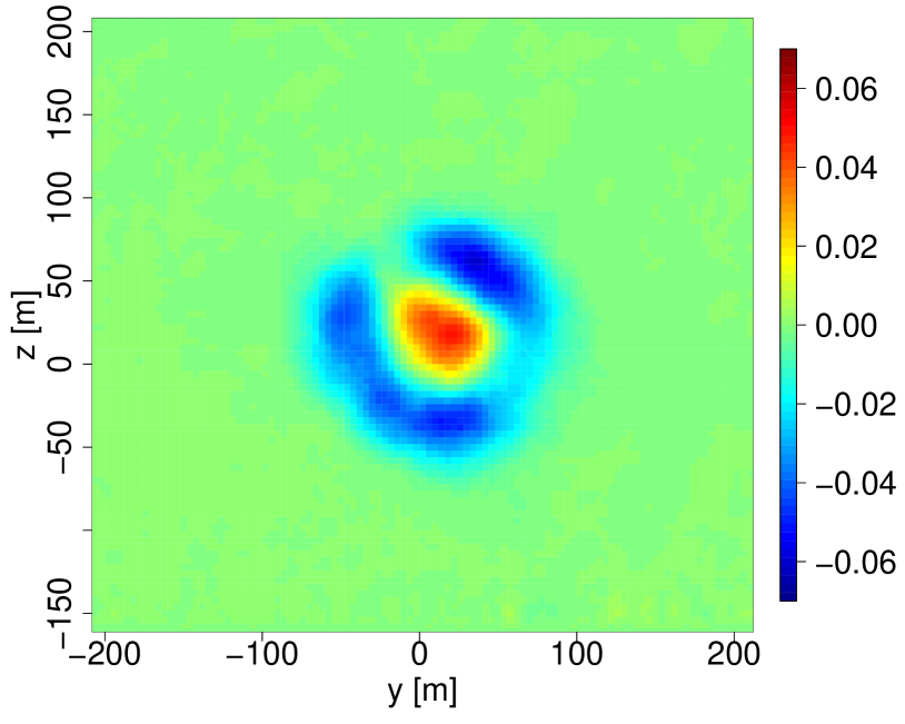
(g)

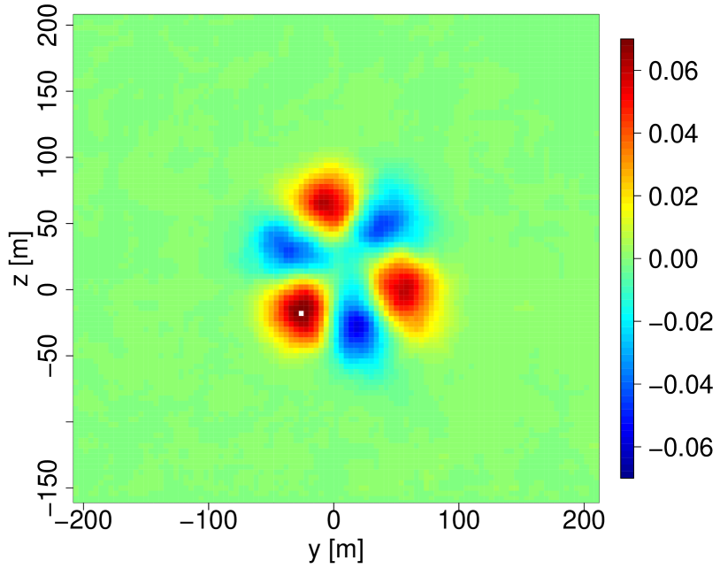
(h)

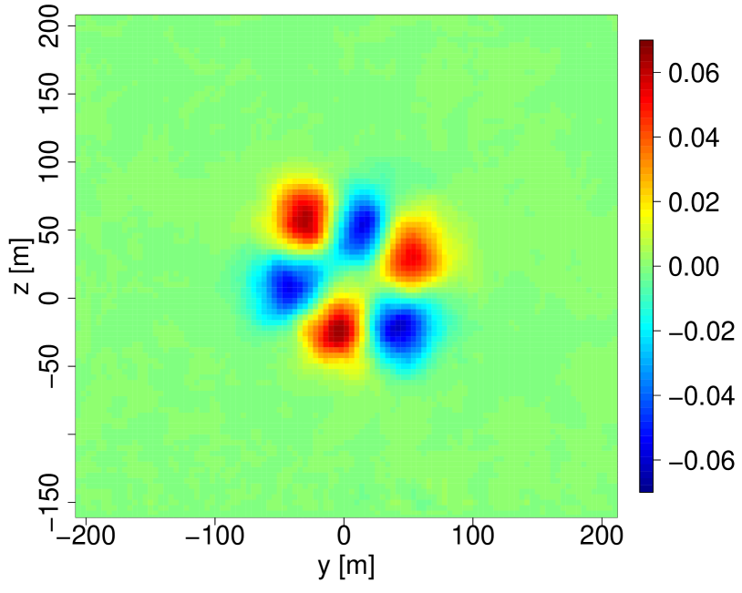
(i)

Figure 3: Mean field and POD modes of the preprocessed field $\tilde{u}$. (a) Mean field; (b) Mode 1; (c) Mode 2; (d) Mode 3; (e) Mode 4; (f) Mode 5; (g) Mode 6; (h) Mode 7; (i) Mode 8.

The modes resemble Fourier modes in the azimuthal direction. We find roughly rotationally symmetric Modes $3$ and $6$ and pairs showing a dipole-like structure $(1,2)$, quadrupole structure $(4,5)$ and hexapole structure $(7,8)$. These observations indicate an approximate statistical isotropy Berkooz et al. (1993). This is a remarkable result, since the rotational symmetry is clearly broken by the ABL. The extracted wake structure therefore behaves approximately isotropic in the non-isotropic ABL flow. Obviously, the rotational symmetry is not perfect. Mode $3$, for example, also indicates the presence of principal axes that do not coincide with the horizontal and vertical direction. Furthermore, the eigenmode pairs described above do not correspond to the same eigenvalue (see Figure 4(a)).

It is important to note that the symmetric properties of the wake structure are revealed through the threshold applied to the field. The original field includes more information about the spatial interaction region between wake and ABL. Consequently, the original field behaves less isotropic, which can also be seen in the corresponding POD modes, as described in Appendix A.

To illustrate the importance of the different modes, we show the POD spectrum and its cumulative version in Figure 4. According to Equation (8), these figures reveal that we need around $100$ modes to recover around 80% of the turbulent kinetic energy of the field $\tilde{u}$. This is not surprising, since in a turbulent flow, the energy is spread out over a wide range of scales. The POD basis does not solve this problem, even though it might perform better in inhomogeneous fields than a standard Fourier basis.

The convergence behavior of the POD modes and values is discussed briefly in Appendix B.

(a)

(b)

Figure 4: (a) POD eigenvalues of the preprocessed field $\tilde{u}$; (b) cumulative energy versus the number of modes $N$.

3.5 Reconstructions of the Velocity Field

We now use the extracted POD modes $\tilde{\phi_{j}}$ to approximate the original field $u(y,z,t)$ according to Equation (9) and vary the number of modes $N$ used for the reconstruction. Examining the reconstructed snapshots (Figure 5), we see that more modes obviously lead to a more accurate description of the wake structure. To recover the spatial small-scale structures of the wake, many POD modes are necessary. Unfortunately, this pure visualization does not offer many clues for the number of modes necessary to obtain a useful low order description. The slow increase of the recovered turbulent kinetic energy with $N$, discussed in the former section, indicates that useful reduced order models need to contain a lot of modes. However, in the context of wake modeling, we are also interested in other quantities describing the impact of the turbine on the wake. Therefore, we propose the use of other quantitative measures of quality in the next section.

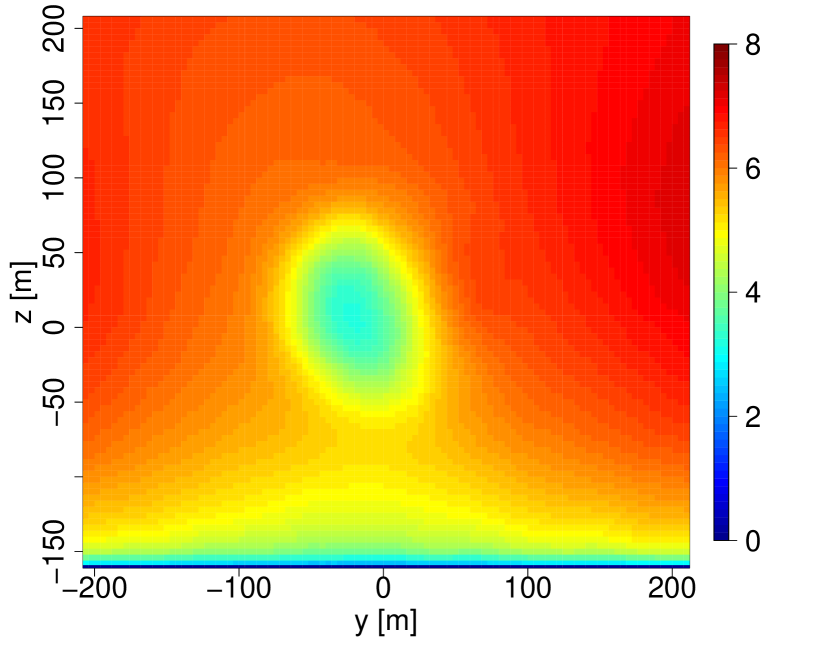
(a)

(b)

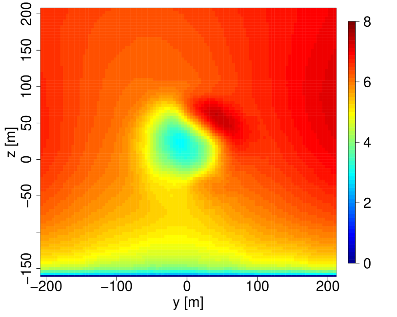
(c)

(d)

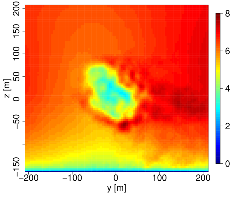
(e)

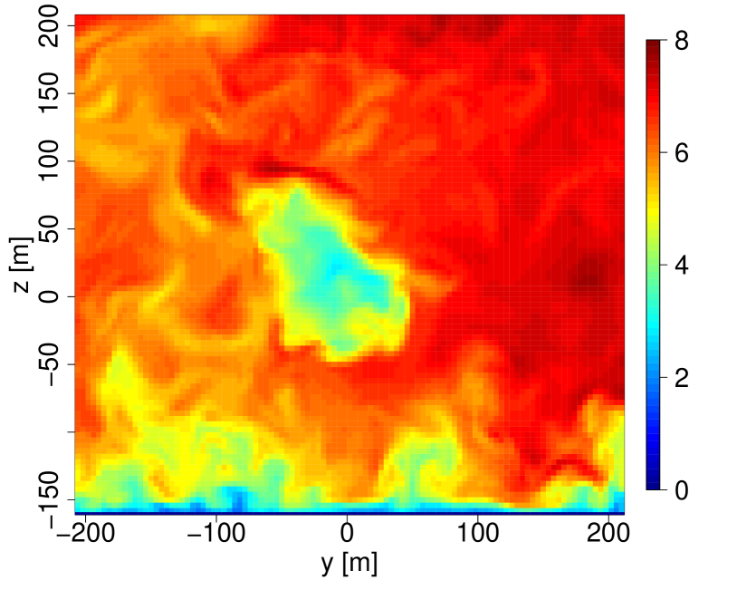
(f)

Figure 5: Reconstructions of the velocity field $u$ following Equation (9) ($t$ = 1000 s). (a) Two modes; (b) three modes; (c) six modes; (d) 10 modes; (e) 100 modes; (f) full field.

4 Alternative Measures for the Quality of Reconstructions

4.1 A General Quality Measure

Our main interest lies in the impact of the wake on a sequential turbine. A measure used to draw conclusions on the quality of a reconstructed field should therefore be related to forces or other effects on a turbine. Such a measure could, for example, be given by a specific load or the power a turbine would produce if it were standing in the wake. Thus, we define a general scalar quality measure $M(t)$ as the result from a corresponding operator $\mathbf{\hat{M}}$ applied to the velocity field:

$$\mathbf{\hat{M}}[u(y,z,t)]=M(t)~{}$$ (10)

Usually, $M$ will depend on the field $u(y,z,t)$ confined to the virtual rotor area only (Figure 6(a)) and not on the velocity in the rest of the domain. Analogous to Equation (10), we define for a reconstructed field:

$$M^{(N)}(t):=\mathbf{\hat{M}}[u^{(N)}(y,z,t)]~{}$$ (11)

The quality of a reconstructed field can now be evaluated by comparing $M^{(N)}(t)$ and $M(t)$. If $M^{(N)}(t)$ is a good approximation of $M(t)$, a reconstruction with $N$ modes yields a good description of the wake with respect to the measure $M(t)$. To quantify the difference of $M^{(N)}(t)$ and $M(t)$, we define two different errors. The first error is given through the two-norm of the time series:

$$\varepsilon_{\mbox{std}}(N)=\frac{\|M^{(N)}-M\|_{2}}{\|M\|_{2}}~{}$$ (12)

which will be referred to as the standard error in the following. Another possible choice is motivated by the idea that sometimes, not the mean $\langle M\rangle_{t}$ is important, but the fluctuations $M(t)-\langle M\rangle_{t}$. It is, e.g., often assumed that for the calculation of fatigue loads, the influence of the mean is negligible. Hence, we define:

$$\varepsilon_{\mbox{dyn}}(N)=\frac{\|(M^{(N)}-\langle M^{(N)}\rangle_{t})-(M-\langle M\rangle_{t})\|_{2}}{\|M-\langle M\rangle_{t}\|_{2}}~{}\vspace{6pt}$$ (13)

which will be referred to as the dynamical error in the following.

4.2 Introducing Alternative Measures

We now define four different measures as $M(t)$, which are related to the power output or forces on a sequential turbine. For this purpose, we take the turbine as a disk in the wake, as shown in Figure 6(a). The first quantity that we analyze is the effective velocity, which we define as the average velocity over the disk area:

$$u_{\mbox{eff}}(t):=\frac{1}{A}\int\limits_{disk}\int\limits dydz~{}u(y,z,t)=~{}\langle u(y,z,t)\rangle_{disk}~{}$$ (14)

where $\langle...\rangle_{disk}$ now plays the role of the operator $\mathbf{\hat{M}}$ in Equation (10). In the spirit of actuator disk theory, this quantity is related to the power output by $u_{\mbox{eff}}^{3}$ and the thrust force on the turbine by $u_{\mbox{eff}}^{2}$.

As a second measure, we use the energy flux through the disk given by:

$$P(t):=\frac{1}{2}\rho A\langle u^{3}(y,z,t)\rangle_{disk}~{}$$ (15)

where $A$ is the area of the disk. $P$ is obviously related to the potential power output of the turbine.

The third measure defined here is related to the torque along the z-axis through the disk (Figure 6(b)) and is defined by:

$$\tau_{z}(t):=\langle u^{2}(y,z,t)\cdot y\rangle_{disk}~{}$$ (16)

where $y$ is the signed distance to the rotational axis. In the case of a wind turbine, the torque in $z$-direction is also called the tower top yaw moment, which is particularly important for the yaw drive of the turbine. In contrast to $u_{\mbox{eff}}$ and $P$, the averaging over the disk is now weighted by $y$, yielding a dependence on the spatial distribution of the deficit over the disk.

The last measure we define is slightly more complex, taking into account that the rotor consists of three rotating blades. We define:

$$T(t):=\int\limits_{blades}\int\limits dydz~{}u^{2}(y,z,t)\propto\langle u^{2}(y,z,t)\rangle_{blades}~{}$$ (17)

where $blades$ denotes the area of the three blades illustrated in Figure 6(c). The blades are rotating with $\omega=10$ rpm, which is a typical value for modern wind turbines. The results presented in this work do not change qualitatively when varying $\omega$ in a realistic range. $T$ is obviously related to the thrust force on a rotor. Since, here, we do not only average over an entire disk, smaller structures of the wake flow become more important.

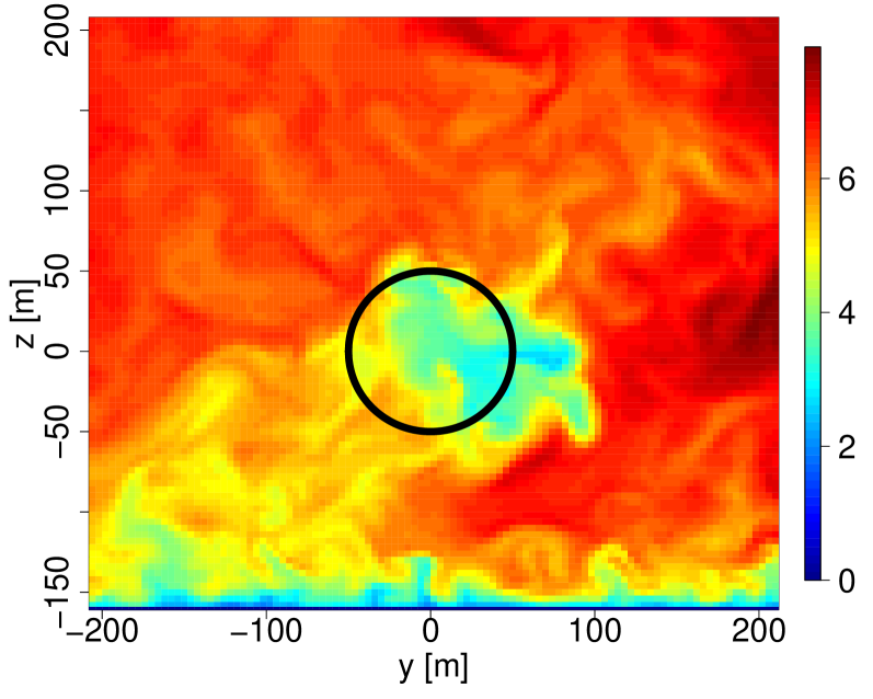
(a)

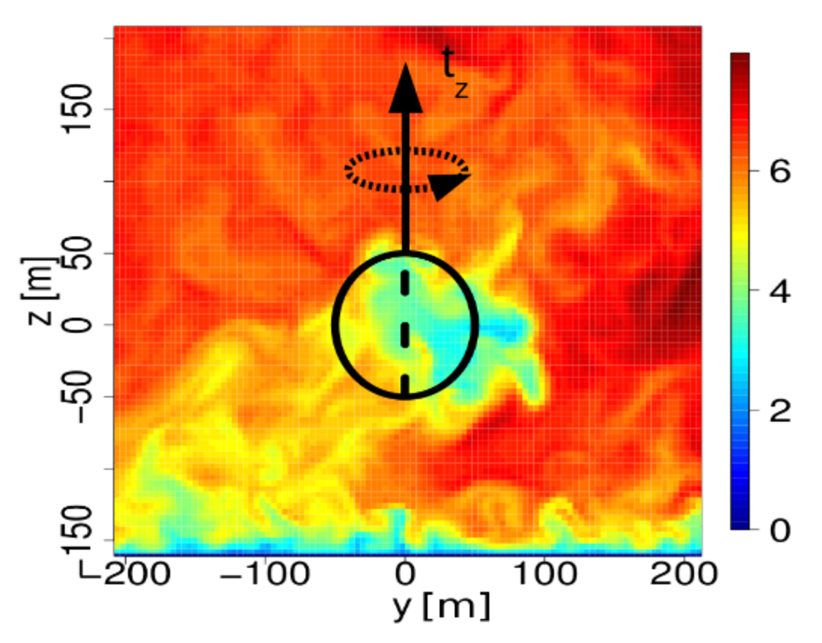
(b)

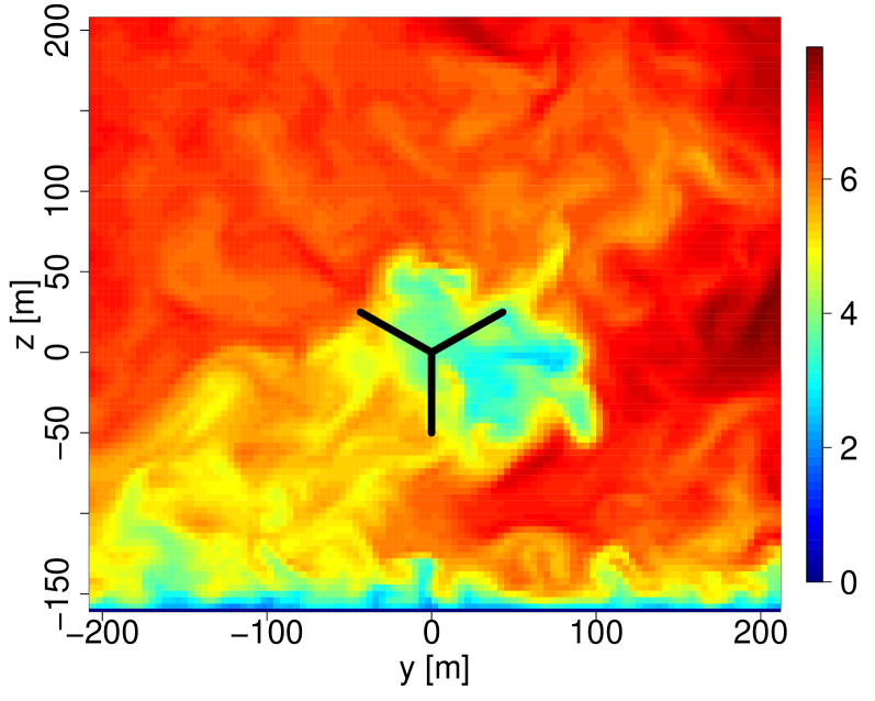
(c)

Figure 6: Illustrations corresponding to the different measures: (a) Measures $u_{\mbox{eff}}$, $P$ and $\tau_{z}$ are obtained through averaging over a disk in the wake flow; (b) $\tau_{z}$ is related to the torque $t_{z}$ on a disk in the flow. The dashed line represents the rotational axis; (c) The measure $T$ results from averaging over three rotor blades in the flow. The blades rotate at 10 rpm.

4.3 Results and Discussion

The measures can now be determined for our data and the corresponding reconstructions described in Section 3.5. In Figures 7 and 8, sections of the time series for $u_{\mbox{eff}}$, $P$, $\tau_{z}$ and $T$ are shown, which we obtained for the original field and reconstructions with different numbers of modes. From these time series, one can already see that the dynamics of $u_{\mbox{eff}}$, $P$ and $T$ cannot be captured using two or less modes, but already, three modes grasp the basic dynamic features. For $\tau_{z}$, basic dynamical aspects are already captured when including only the first mode (Figure 8(b)).

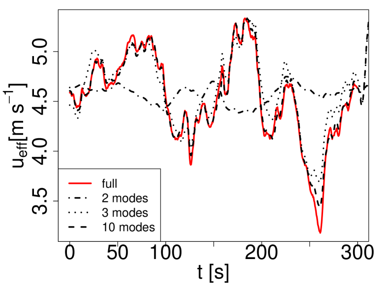
(a)

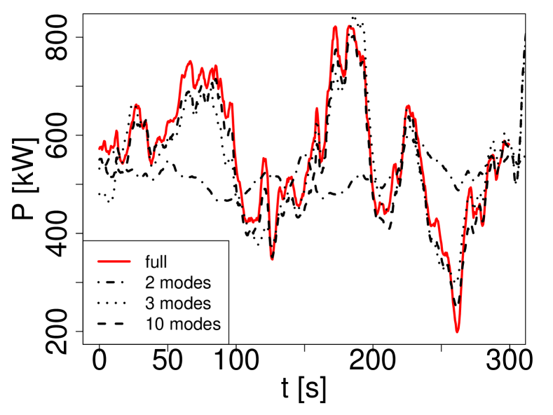
(b)

Figure 7: The measures (a) $u_{\mbox{eff}}$ and (b) $P$ for different numbers of modes used for the POD reconstructions.

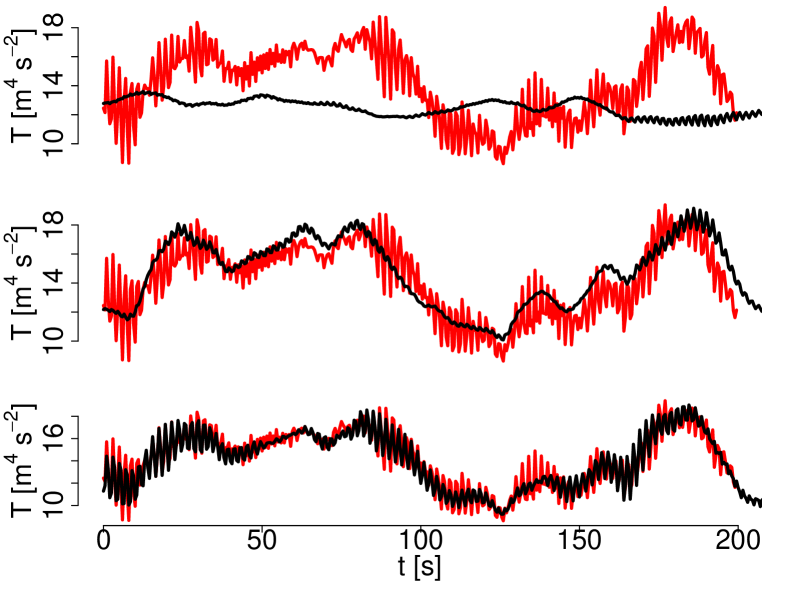
(a)

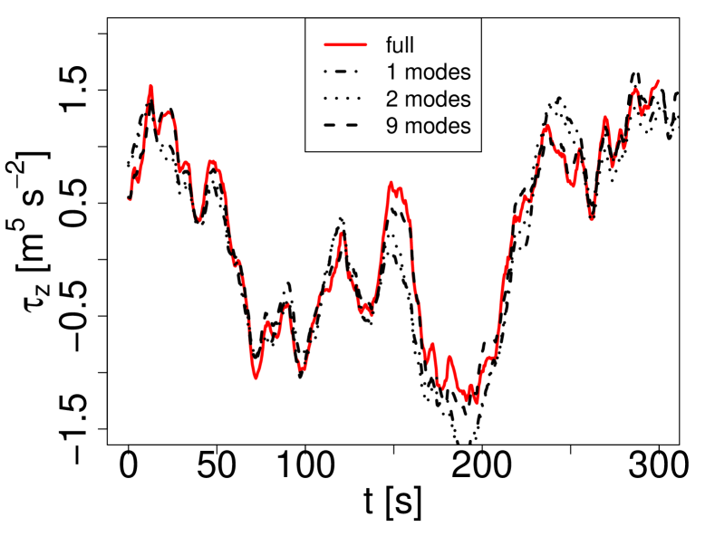
(b)

Figure 8: (a) The measure $T$ for different numbers of modes used for the reconstruction. The red lines show $T$ for the original field, while the black line shows $T$ of a reconstructed field ((top) two modes; (middle) three modes; (bottom) $10$ modes); (b) Dynamics of the measure $\tau_{z}$ for different numbers of modes used for the reconstruction. Note that since the reconstruction is already quite good with one mode, the lines lie almost on top of each other. However, there is still a visible improvement in the case of nine modes.

4.3.1 Behavior of the Dynamical and Standard Error

The differences between the time series of the original field and the reconstructions can now be quantified by the errors $\varepsilon_{\mbox{dyn}}$ and $\varepsilon_{\mbox{std}}$ shown in Figure 9. We start with a discussion of the dynamical error $\varepsilon_{\mbox{dyn}}$, followed by a comparison with $\varepsilon_{\mbox{std}}$.

(a)

(b)

Figure 9: (a) Dynamical and (b) standard error for different measures versus the number $N$ of modes used for reconstruction. $N=0$ corresponds to a reconstruction with the mean field only.

As expected from the inspection of the time series of $u_{\mbox{eff}}$, $P$ and $T$, $\varepsilon_{\mbox{dyn}}$ shows a sudden decline from above 80% to below 20% when including the third mode (Figure 9(a)). For $\tau_{z}$, $\varepsilon_{\mbox{dyn}}$ goes down to below 20% when only the first mode is included. Increasing to six modes results in a further reduction of the dynamical error to less than 10% for $u_{\mbox{eff}}$ and $P$, about 10% for $\tau_{z}$ and around 20% for $T$.

Another remarkable result, revealed in Figure 9(a), is the discontinuous decay of $\varepsilon_{\mbox{dyn}}$. The most pronounced jumps occur for $u_{\mbox{eff}}$, $P$ and $T$ when including Mode $3$ and for $\tau_{z}$ when including the first mode. The improvement of the error when including a mode might be seen as an indicator of its importance. The jump with Mode $3$ therefore indicates that the third mode plays a special role for the description of $u_{\mbox{eff}}$, $P$ and $T$, while the first mode is of major importance for $\tau_{z}$. This will be discussed further in Section 4.3.2.

The similar performance of $u_{\mbox{eff}}$, $P$ and $T$, particularly the sudden jump with the third mode, is probably caused by the fact that all three measures are integrated over the whole rotor or blade area without any specific weighting. It seems to be of minor importance whether we integrate over $u$, $u^{2}$ or $u^{3}$. The slightly weaker performance of $T$, especially with more modes, probably results from the integration over the smaller blade area. Therefore, smaller structures are important for the dynamics of $T$, which cannot be resolved by only a few modes. This can also be seen in the time series in Figure 8(a), where three modes nicely recover the macroscopic behavior of $T$, but $10$ modes still fail to grasp some of the finer structures of the signal. The distinct behavior of $\varepsilon_{\mbox{dyn}}$ for $\tau_{z}$ is likely to be caused by the weighting with the signed distance to the rotational axis. Due to this weighting, modes symmetric to the rotational axis become less relevant than antisymmetric modes.

The standard error shows the same discontinuous behavior as the dynamical one with jumps at identical numbers of modes as identified for $\varepsilon_{\mbox{dyn}}$ (Figure 9(b)). However, two major differences can be found. The first difference is that for $u_{\mbox{eff}}$, $P$ and $T$, the standard error is already very low when only using the mean field of the flow, with around 10% for $u_{\mbox{eff}}$ and 20% for $P$. The second is the generally weaker performance of $\tau_{z}$. This different behavior stems from the fact that $\varepsilon_{\mbox{dyn}}$ neglects the mean values of the measures in contrast to $\varepsilon_{\mbox{std}}$ (compare Equations (12) and (13)). For $u_{\mbox{eff}}$, $P$ and $T$ the steady mean field without any modes already yields a good description of the mean values of $u_{\mbox{eff}}$, $P$ and $T$. Since the mean values of these measures are larger than the fluctuating parts, this yields the small standard error in Figure 9(b). Further details, also on the behavior of $\tau_{z}$, can be found in Appendix C.

4.3.2 Selection of Modes

So far, we included the extracted modes ordered from high to low energy content, as usual for POD reconstructions. In the previous section, Section 4.3, we already noted that the discontinuous behavior of the reconstruction error indicates that different modes are relevant for different measures. This naturally suggests choosing only modes that correspond to jumps in the errors when focusing on a specific measure.

The first example for this approach can be seen in Figure 10. The third mode, which corresponds to a sharp decrease in the error of $u_{\mbox{eff}}$, yields a better reconstruction of $u_{\mbox{eff}}$ than the first mode. In the second example (Figure 11), the measure $\tau_{z}$ is reconstructed choosing two different sets of modes. The performance of the modes $(1,6,10)$, which correspond to sharp decreases in both errors (see Figure 9), yields a better approximation of $\tau_{z}$ than the most energetic modes $(1,2,3)$.

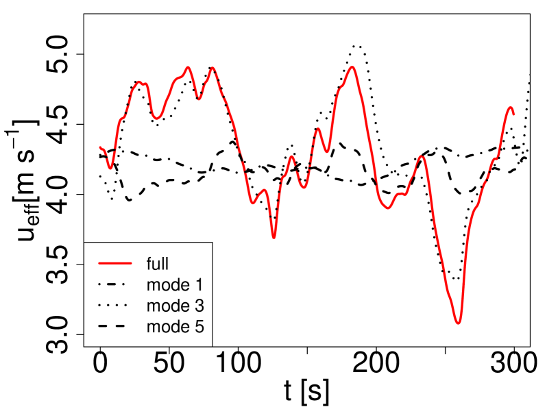
(a)

(b)

Figure 10: (a) Effective velocity $u_{\mbox{eff}}$ for different reconstructions of $u(y,z,t)$ using only one single mode (plus mean field); (b) dynamical error for reconstructions using a single mode only. The $x$-axis denotes the number of the mode used for the reconstruction.

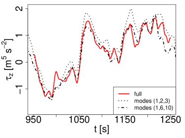
Figure 11: Torque-related measure $\tau_{z}$ for the original field and two reconstructions using a different set of three modes.

From these results, we can conclude that the usual energetic order is not necessarily the best choice for other measures than the turbulent kinetic energy. Finding the optimal modes can therefore improve the results or reduce the necessary dimension when aiming for the description of a specific quantity. It is important to note that the sharp decreases in the errors can, in general, only be a first indicator for the importance of the modes, since most measures of interest are nonlinear. An alternative idea to find the optimal modes could be to take symmetry considerations into account, as indicated above for $\tau_{z}$ in Section 4.3.1 and proposed by Saranyasoontorn and Manuel Saranyasoontorn and Manuel (2006).

5 Interpretation of the Modes

For a better understanding of the results in the last section, we now relate the first three POD modes to the dynamical properties of the wake deficit.

5.1 Meandering

The first dynamical property that we analyze is the meandering or large-scale movement of the velocity deficit. For this purpose, we determine the center of the deficit as:

$$\left(\begin{array}[]{c}y_{c}(t)\\ z_{c}(t)\end{array}\right):=\frac{\int\limits dydz~{}\tilde{u}^{2}(y,z,t)\left(\begin{array}[]{c}y\\ z\end{array}\right)}{\int\limits dydz~{}\tilde{u}^{2}(y,z,t)}~{}$$ (18)

which we evaluate for every time step. The definition can be interpreted as the center of energy of the deficit. Other approaches have been used in the literature España et al. (2011); Trujillo et al. (2011); Muller et al. (2013), but for these data, Equation (18) yielded the most robust results.

To investigate the relation to the POD modes, we compare the trajectories of the center to the weighting coefficients $a_{j}(t)$ of the POD modes. The horizontal trajectory is strongly correlated with the amplitude of the first mode (Figure 12(a)), yielding a linear correlation coefficient of $\rho(y_{c},a_{1})=0.84$ (Figure 12(b)). The correlations to other weighting coefficients are almost negligible. Analogously, we find $\rho(z_{c},a_{2})=0.81$ for the vertical movement and the second amplitude (Figure 13). Thus, the first and second mode are related to the horizontal and vertical movement, respectively. To support the former arguments, Figure 14 shows the horizontal position for the original field and different reconstructions. One mode actually grasps the horizontal low amplitude movement of the deficit. To recover the high amplitudes, more modes need to be included.

The connection of the first mode to the horizontal meandering also yields a deeper understanding of the behavior of the measure $\tau_{z}$. The torque in the z-direction and, thus, $\tau_{z}$ are obviously strongly influenced by the horizontal position of the deficit. A large movement to the right, for example, yields a strongly asymmetric force on the disk, inducing a positive torque in the $z$-direction. Since one mode is enough to capture the basic dynamics of the horizontal movement, it is also sufficient for an approximate description of $\tau_{z}$. Analogous arguments can also be made for the second mode and the vertical meandering, which induces torque in the $y$-direction.

(a)

(b)

Figure 12: (a) Time series of the first weighting coefficient $a_{1}$ and the horizontal position of the deficit $y_{c}$; (b) correlation coefficients $\rho$ of the horizontal deficit position $y_{c}$ with the weighting coefficients of the first 10 modes.

(a)

(b)

Figure 13: (a) Time series of the second weighting coefficient $a_{2}$ and the vertical position of the deficit $z_{c}$; (b) correlation coefficients $\rho$ of the horizontal deficit position $z_{c}$ with the weighting coefficients of the first 10 modes.

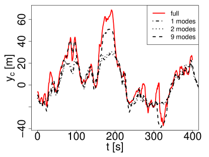
Figure 14: The horizontal position of the deficit $y_{c}$ for different reconstructions of $u(y,z,t)$ using different numbers of modes.

5.2 Amplitude

As the third dynamical property of the deficit, we investigate the average amplitude of the deficit, which we define as the velocity spatially averaged over the complete deficit (extracted through the threshold application). As before, we compare the time series of this amplitude to the weighting coefficients of the modes and calculate the corresponding correlation coefficients. Figure 15 shows that this amplitude is strongly (anti-) correlated to the third weighting coefficient with $\rho=-0.64$. Since the third mode is very important for recovering the measures $u_{\mbox{eff}}$, $P$ and $T$, the average amplitude probably plays a major role for the power output and thrust on a turbine. Therefore, only considering the meandering is not enough to describe these quantities.

(a)

(b)

Figure 15: (a) Time series of the third weighting coefficient $a_{3}$ and the average amplitude of the deficit (called amp in the figure); (b) correlation coefficients $\rho$ of the average amplitude of the deficit with the weighting coefficients of the first 10 modes.

6 Conclusions

A modified POD analysis has been applied to the large eddy simulation of an actuator disk in a turbulent atmospheric boundary layer. The main goal of this work was to identify modes that yield a strong dimensional reduction of the wake flow. Such a reduction would facilitate the application of low dimensional modeling methods to the temporal dynamics of the weighting coefficients of the modes.

Based on our results, we propose that the quality of modal reconstructions of the field should not only be assessed by considering the recovery of turbulent kinetic energy, but should be based on quantities relevant to a sequential turbine in the wake. The basic dynamics of such relevant quantities (e.g., the energy flux through a disk) could already be captured using the three most energetic modes of our analysis. This strong dimensional reduction of the flow indicates that developing wake models of very low order is possible. Therefore, these results strongly support the idea of building simplified dynamic wake models based on a superposition of spatial modes. Such models could be a useful alternative to dynamic models mainly based on the meandering process. They could therefore play an important role for the layout optimization and controlling of wind farms. Furthermore, our results support the idea of simplified dynamic wake models in general, since we show that relevant information is contained in only a few degrees of freedom.

A further dimensional reduction could possibly be achieved when a wake model is used to describe a very specific impact on a sequential turbine (e.g., the tower top yaw moment), since our results suggest that the necessary level of complexity depends on the quantity that we aim to describe. Furthermore, we showed that including modes in the usual energetic order is not generally the best choice. Thus, modes could be chosen with respect to the application, neglecting irrelevant modes, despite a possible high energy content.

We showed that relating spatial modes to specific properties of the wake can yield a deeper understanding of models based on modal decompositions. This interpretation can reveal relations to features of other dynamic wake models. In our case, a description with the first two POD modes is related to a dynamic wake model, which includes meandering as its only dynamic feature. The importance of Mode $3$ and, thus, the average amplitude of the wake indicates that meandering alone might not be sufficient to capture the basic dynamics of, e.g., the thrust on the turbine. Therefore, a fluctuating amplitude might be a useful extension to a pure meandering model of the wake.

The modes that we obtained after applying a threshold to the field had features corresponding to a statistically rotationally symmetric field. Since these modes performed well, this slightly supports an approach also used in dynamic wake meandering models, where an axial-symmetric wake is assumed before including the ABL. It might therefore be possible to model the wake and ABL separately and include possible interactions at a different level.

To show the robustness of our results, this study could obviously benefit from the analysis of additional datasets, such as more detailed simulations or high-speed PIVdata from wind tunnel experiments. The quality measures introduced, even though related to the performance of a turbine in the wake, are simple. Therefore, an aeroelastic code could be used, as a next step, to obtain better measures of quality. Another possible improvement of models based on decompositions could be achieved by including all three velocity components. However, it is not clear whether a sufficient dimensional reduction is possible in this case.

So far, we have mainly investigated the quality of the reduced descriptions of the wake dynamics. Building a reduced order model based on the extracted POD modes is a very challenging task; since we need to model the temporal dynamics of the weighting coefficients of the modes. To do this, we plan to consider the weighting coefficients as stochastic processes and to estimate the corresponding model equations in the spirit of, e.g., Kleinhans and Friedrich (2007); Friedrich et al. (2011); Milan et al. (2014).

Appendix A POD Modes without a Threshold

In this Appendix, we describe the POD modes obtained without applying any kind of preprocessing and discuss the corresponding results for the different quality measures used in Section 4.

When not using the threshold as introduced in Section 3.3, the POD modes and values strongly depend on the spatial region used for the analysis. Here, we chose the region $[-120,120]$ m $\times$ $[-120,120]$ m centered at the hub height to apply the POD. It should be noted that some of the modes were sensitive even to relatively small changes of the size of this window.

The obtained modes are shown in Figure A1. Some modes are quite similar to the modes obtained after preprocessing (compare to Figure 3). For example, Mode $1$ stays almost the same, and Mode $7$ resembles the former Mode $4$. Other modes, like Mode $4$ or Mode $8$, appear slightly more complex. Generally, we can say that the modes appear less clearly structured, even though some of the azimuthal structures are retained.

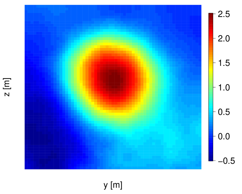
(a)

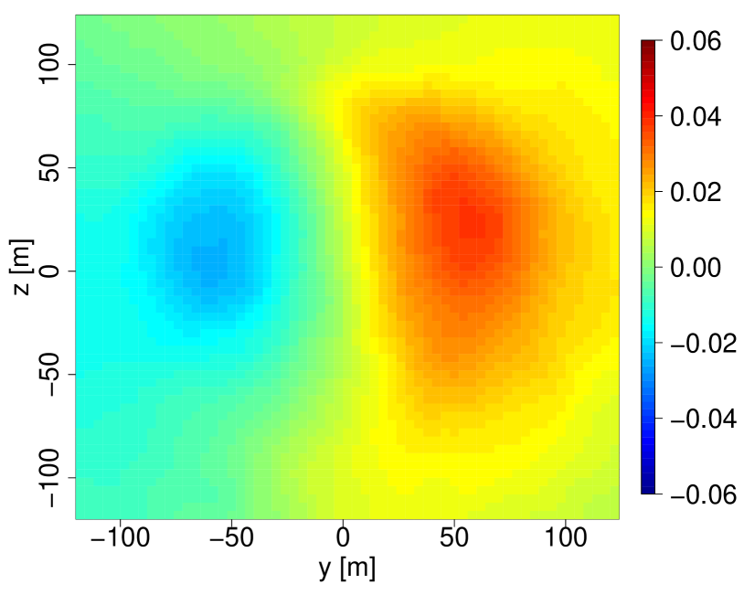
(b)

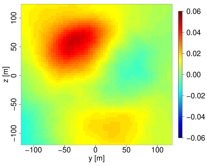
(c)

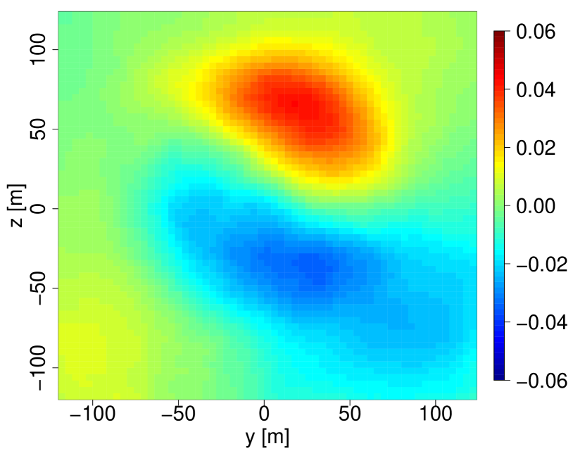
(d)

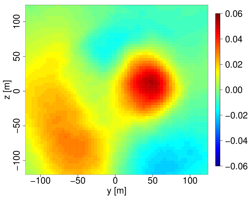
(e)

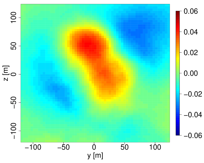
(f)

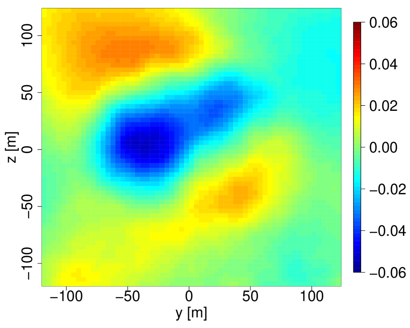
(g)

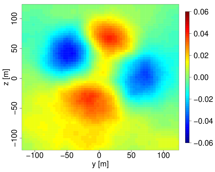
(h)

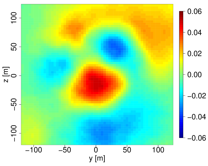
(i)

Figure A1: Mean field and POD modes. (a) Mean field; (b) Mode 1; (c) Mode 2; (d) Mode 3; (e) Mode 4; (f) Mode 5; (g) Mode 6; (h) Mode 7; (i) Mode 8.

As the next point, we investigate the influence of these new modes on the quality of reconstructions with the measures defined in Section 4. In Figure A2, the corresponding error graphs are shown. The major difference is the steady decrease of the dynamical error for $u_{\mbox{eff}}$, $P$ and $T$. The sudden jumps are missing. Particularly, the large decrease with the third mode has vanished (compare with Figure 9(a)). Therefore, a model based on less than six modes would probably perform worse when using the modes obtained without a threshold.

(a)

(b)

Figure A2: (a) Dynamical and (b) standard error for different measures versus the number $N$ of modes used for the reconstruction. $N=0$ corresponds to a reconstruction with the mean field only.

Appendix B Convergence Study of POD Modes and Values

In this appendix, we briefly discuss the convergence behavior of the POD modes and the values presented in Section 3.4. For this purpose, we investigate the sensitivity of these results to the number of snapshots used for their estimation. In Figure B1, the behavior of two different eigenvalues is illustrated. After around 11,000 snapshots, the change when including more snapshots stays below 5%. Thus, the values are roughly converged. Note that less independent snapshots would be necessary due to the temporal correlations in the field.

Figure B2 illustrates the change of the estimate of Mode $4$ when increasing the number of snapshots. The basic structure is already visible after around 1000 snapshots. After around 6000, no strong changes in the mode are visible anymore. Similar results have been found for the other modes, but the convergence of the modes gets weaker with higher mode number. These results indicate that the modes used for the reconstructions in this paper are converged and will not change strongly when using longer simulations.

(a)

(b)

Figure B1: Eigenvalue versus the number of snapshots used for its estimation. (a) First eigenvalue (n = 1); (b) second eigenvalue (n = 2).

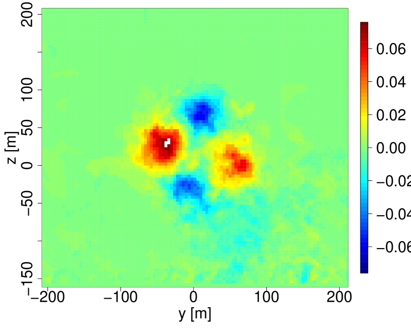
(a)

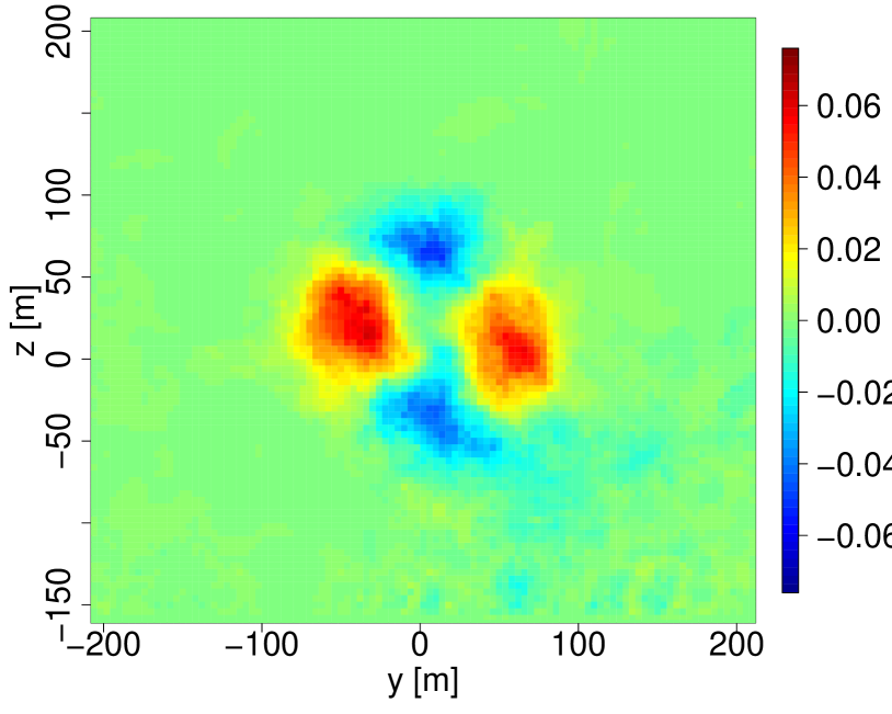
(b)

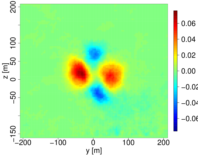
(c)

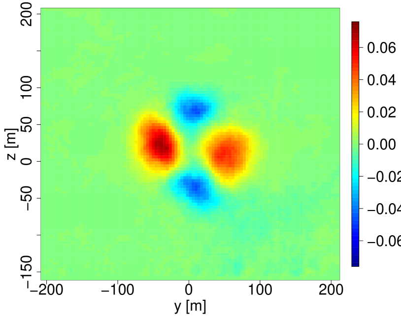
(d)

Figure B2: Fourth POD mode estimated using different numbers of snapshots: (a) 1000; (b) 2000; (c) 6000; (d) 10,000.

Appendix C Further Explanations on the Standard Error

In this Appendix, the discussion in Section 4.3 about the results for the standard error (Figure 9(b)) is continued. We start by illustrating why the standard error is already low for $u_{\mbox{eff}}$ and $P$ when using only the mean field followed by a comparison with $\tau_{z}$.

For $u_{\mbox{eff}}$, using only the steady mean field already yields a perfect reconstruction of $\langle u_{\mbox{eff}}\rangle_{t}$:

$$\langle\langle u(y,z,t)\rangle_{t}\rangle_{disk}=\langle\langle u(y,z,t)\rangle_{disk}\rangle_{t}=\langle u_{\mbox{eff}}(t)\rangle_{t}~{}$$ (C1)

Since the fluctuations of $u_{\mbox{eff}}$ are much smaller than the mean value, the correct description of the mean obviously leads to a low standard error (see Equation (12)), due to the normalization. For the dynamical error (Equation (13)), the recovery of the mean obviously does not play any role. For $P$, $\langle P\rangle_{t}$ cannot be fully recovered using just $\langle u(y,z,t)\rangle_{t}$ due to:

$$\langle\langle u\rangle_{t}^{3}\rangle_{disk}\neq\langle\langle u^{3}\rangle_{t}\rangle_{disk}=\langle\langle u^{3}\rangle_{disk}\rangle_{t}\propto\langle P\rangle_{t}$$ (C2)

Consequently, the standard error is always higher for $P$ than for $u_{\mbox{eff}}$. Similarly, we have for $\tau_{z}$:

$$\langle\langle u\rangle_{t}^{2}y\rangle_{disk}\neq\langle\langle u^{2}\rangle_{t}y\rangle_{disk}=\langle\langle u^{2}y\rangle_{disk}\rangle_{t}=\langle\tau_{z}\rangle_{t}~{}$$ (C3)

For $\tau_{z}$, the fluctuations are much higher than for $P$. This yields a large difference between $\langle u\rangle_{t}^{2}$ and $\langle u^{2}\rangle_{t}$, resulting in the large standard error compared with $P$ and $u_{\mbox{eff}}$. Similar arguments can be found for $T$.

The short discussion above does not only explain the different behavior of $\varepsilon_{\mbox{dyn}}$ and $\varepsilon_{\mbox{std}}$, but also nicely illustrates a major challenge for steady mean field models. Since the conversion from wind to relevant quantities, such as power or loads, can be a nonlinear process, the mean velocity field does not necessarily offer a good description of other mean quantities.

Conflicts of Interest

The authors declare no conflict of interest.

References

- Barthelmie et al. (2010) Barthelmie, R.J.; Pryor, S.C.; Frandsen, S.T.; Hansen, K.S.; Schepers, J.G.; Rados, K.; Schlez, W.; Neubert, A.; Jensen, L.E.; Neckelmann, S. Quantifying the impact of wind turbine wakes on power output at offshore wind farms. J. Atmos. Ocean. Technol. 2010, 27, 1302–1317.
- Goit and Meyers (2014) Goit, J.P.; Meyers, J. Analysis of turbulent flow properties and energy fluxes in optimally controlled wind-farm boundary layers. J. Phys. Conf. Ser. 2014, 524, doi:10.1088/1742-6596/524/1/012178.
- Storey et al. (2014) Storey, R.C.; Norris, S.E.; Cater, J.E. Modelling turbine loads during an extreme coherent gust using large eddy simulation. J. Phys. Conf. Ser. 2014, 524, doi:10.1088/1742-6596/524/1/012177.
- Medici (2005) Medici, D. Experimental Studies of Wind Turbine Wakes: Power Optimisation and Meandering. Ph.D. Thesis, KTH Mechanics, Royal Institute of Technology, Stockholm, Sweden, 2005.
- Jimenez et al. (2010) Jimenez, A.; Crespo, A.; Migoya, E. Application of a LES technique to characterize the wake deflection of a wind turbine in yaw. Wind Energy 2010, 13, 559–572.
- Fleming et al. (2014) Fleming, P.A.; Gebraad, P.M.O.; Lee, S.; van Wingerden, J.W.; Johnson, K.; Churchfield, M.; Michalakes, J.; Spalart, P.; Moriarty, P. Evaluating techniques for redirecting turbine wakes using SOWFA. Renew. Energy 2014, 70, 211–218.
- Pope (2000) Pope, S.B. Turbulent Flows; Cambridge University Press: Cambridge, UK, 2000.
- Jimenez et al. (2007) Jimenez, A.; Crespo, A.; Migoya, E.; Garcia, J. Advances in large-eddy simulation of a wind turbine wake. J. Phys. Conf. Ser. 2007, 75, doi:10.1088/1742-6596/75/1/012041.
- Calaf et al. (2010) Calaf, M.; Meneveau, C.; Meyers, J. Large eddy simulation study of fully developed wind-turbine array boundary layers. Phys. Fluids 2010, 22, doi:10.1063/1.3291077.
- Porté-Agel et al. (2011) Porté-Agel, F.; Wu, Y.T.; Lu, H.; Conzemius, R.J. Large-eddy simulation of atmospheric boundary layer flow through wind turbines and wind farms. J. Wind Eng. Ind. Aerodyn. 2011, 99, 154–168.
- Witha et al. (2014) Witha, B.; Steinfeld, G.; Heinemann, D. High-resolution offshore wake simulations with the LES model PALM. In Wind Energy-Impact of Turbulence; Springer: Berlin, Germany, 2014; pp. 175–181.
- Jensen (1983) Jensen, N.O. A Note on Wind Generator Interaction; Risø-M-2411; Riso National Laboratory: Roskilde, Denmark, 1983.
- Ainslie (1988) Ainslie, J.F. Calculating the flowfield in the wake of wind turbines. J. Wind Eng. Ind. Aerodyn. 1988, 27, 213–224.
- Larsen (1988) Larsen, G.C. A Simple Wake Calculation Procedure; Riso National Laboratory: Roskilde, Denmark, 1988.
- Frandsen (2003) Frandsen, S. Turbulence and Turbulence Generated Fatigue in Wind Turbine Clusters; Riso Report R-1188; Riso National Laboratory: Roskilde, Denmark, 2003.
- Frandsen et al. (2006) Frandsen, S.; Barthelmie, R.; Pryor, S.; Rathmann, O.; Larsen, S.; Hojstrup, J.; Thogersen, M. Analytical modelling of wind speed deficit in large offshore wind farms. Wind Energy 2006, 9, 39–53.
- Schmidt (2014) Schmidt, J., S.B. Wind farm layout optimisation using wakes from computational fluid dynamics simulations. In Proceedings of the EWEA Conference, Barcelona, Spain, 10–13 March 2014.
- Larsen et al. (2007) Larsen, G.C.; Madsen Aagaard, H.; Bingöl, F.; Mann, J.; Ott, S.; Sørensen, J.N.; Okulov, V.; Troldborg, N.; Nielsen, N.M.; Thomsen, K. Dynamic Wake Meandering Modeling; Riso National Laboratory: Roskilde, Denmark, 2007.
- Larsen et al. (2008) Larsen, G.C.; Madsen, H.A.; Thomsen, K.; Larsen, T.J. Wake meandering: A pragmatic approach. Wind Energy 2008, 11, 377–395.
- Trujillo et al. (2011) Trujillo, J.J.; Bingol, F.; Larsen, G.C.; Mann, J.; Kuehn, M. Light detection and ranging measurements of wake dynamics. Part II: Two-dimensional scanning. Wind Energy 2011, 14, 61–75.
- España et al. (2012) España, G.; Aubrun, S.; Loyer, S.; Devinant, P. Wind tunnel study of the wake meandering downstream of a modelled wind turbine as an effect of large scale turbulent eddies. J. Wind Eng. Ind. Aerodyn. 2012, 101, 24–33.
- Thomsen and Madsen (2005) Thomsen, K.; Madsen, H.A. A new simulation method for turbines in wake—Applied to extreme response during operation. Wind Energy 2005, 8, 35–47.
- Thomsen et al. (2007) Thomsen, K.; Madsen, H.A.; Larsen, G.C.; Larsen, T.J. Comparison of methods for load simulation for wind turbines operating in wake. J. Phys. Conf. Ser. 2007, 75, doi:10.1088/1742-6596/75/1/012072.
- Andersen et al. (2013) Andersen, S.J.; Sorensen, J.N.; Mikkelsen, R. Simulation of the inherent turbulence and wake interaction inside an infinitely long row of wind turbines. J. Turbul. 2013, 14, 1–24.
- Berkooz et al. (1993) Berkooz, G.; Holmes, P.; Lumley, J.L. The proper orthogonal decomposition in the analysis of turbulent flows. Annu. Rev. Fluid Mech. 1993, 25, 539–575.
- Citriniti and George (2000) Citriniti, J.; George, W. Reconstruction of the global velocity field in the axisymmetric mixing layer utilizing the proper orthogonal decomposition. J. Fluid Mech. 2000, 418, 137–166.
- Jung et al. (2004) Jung, D.; Gamard, S.; George, W.K. Downstream evolution of the most energetic modes in a turbulent axisymmetric jet at high Reynolds number. Part 1. The near-field region. J. Fluid Mech. 2004, 514, 173–204.
- Iqbal and Thomas (2007) Iqbal, M.O.; Thomas, F.O. Coherent structure in a turbulent jet via a vector implementation of the proper orthogonal decomposition. J. Fluid Mech. 2007, 571, 281–326.
- Tutkun et al. (2008) Tutkun, M.; Johansson, P.V.; George, W.K. Three-component vectorial proper orthogonal decomposition of axisymmetric wake behind a disk. AIAA J. 2008, 46, 1118–1134.
- Delville et al. (1999) Delville, J.; Ukeiley, L.; Cordier, L.; Bonnet, J.P.; Glauser, M. Examination of large-scale structures in a turbulent plane mixing layer. Part 1. Proper orthogonal decomposition. J. Fluid Mech. 1999, 391, 91–122.
- Bergmann et al. (2005) Bergmann, M.; Cordier, L.; Brancher, J.P. Optimal rotary control of the cylinder wake using proper orthogonal decomposition reduced-order model. Phys. Fluids 2005, 17, doi:10.1063/1.2033624.
- Cordier et al. (2013) Cordier, L.; Noack, B.R.; Tissot, G.; Lehnasch, G.; Delville, J.; Balajewicz, M.; Daviller, G.; Niven, R.K. Identification strategies for model-based control. Exp. Fluids 2013, 54, 1–21.
- Andersen et al. (2014) Andersen, S.J.; Sørensen, J.N.; Mikkelsen, R. Reduced order model of the inherent turbulent flow of wind turbine wakes inside an infinitely long row of turbines. J. Phys. Conf. Ser. 2014, 555, doi:10.1088/1742-6596/555/1/012005.
- Kantz and Schreiber (2004) Kantz, H.; Schreiber, T. Nonlinear Time Series Analysis; Cambridge University Press: Cambridge, UK, 2004; Volume 7.
- Argyris et al. (2010) Argyris, J.H.; Faust, G.; Friedrich, R.; Haase, M. An Exploration of Dynamical Systems and Chaos; Springer: Berlin, Germany, 2015.
- Kleinhans and Friedrich (2007) Kleinhans, D.; Friedrich, R. Quantitative Estimation of Drift and Diffusion Functions from Time Series Data. In Wind Energy; Springer: Berlin, Germany, 2007; pp. 129–133.
- Friedrich et al. (2011) Friedrich, R.; Peinke, J.; Sahimi, M.; Reza Rahimi Tabar, M. Approaching complexity by stochastic methods: From biological systems to turbulence. Phys. Rep. 2011, 506, 87–162.
- Milan et al. (2014) Milan, P.; Wächter, M.; Peinke, J. Stochastic modeling and performance monitoring of wind farm power production. J. Renew. Sustain. Energy 2014, 6, doi:10.1063/1.4880235.
- Bastine et al. (2014) Bastine, D.; Witha, B.; Wächter, M.; Peinke, J. POD analysis of a wind turbine wake in a turbulent atmospheric boundary layer. J. Phys. Conf. Ser. 2014, 524, doi:10.1088/1742-6596/524/1/012153.
- Saranyasoontorn and Manuel (2005) Saranyasoontorn, K.; Manuel, L. Low-dimensional representations of inflow turbulence and wind turbine response using proper orthogonal decomposition. J. Sol. Energy Eng. 2005, 127, 553–562.
- Saranyasoontorn and Manuel (2006) Saranyasoontorn, K.; Manuel, L. Symmetry considerations when using proper orthogonal decomposition for predicting wind turbine yaw loads. J. Sol. Energy Eng.-Trans. Asme 2006, 128, 574–579.
- Raasch and Schröter (2001) Raasch, S.; Schröter, M. PALM—A large-eddy simulation model performing on massively parallel computers. Meteorol. Z. 2001, 10, 363–372.
- Maronga et al. (2014) Maronga, B.; Gryschka, M.; Heinze, R.; Hoffmann, F.; Kanani-Sühring, F.; Keck, M.; Ketelsen, K.; Letzel, M.O.; Sühring, M.; Raasch, S. The Parallelized Large-Eddy Simulation Model (PALM) version 4.0 for Atmospheric and Oceanic Flows: Model Formulation, Recent Developments and Future Perspectives Geosci. Model Dev. Discuss. 2014, submitted.
- Deardorff (1980) Deardorff, J. Stratocumulus-capped mixed layers derived from a three-dimensional model. Bound.-Layer Meteorol. 1980, 18, 495–527.
- Wu and Porté-Agel (2011) Wu, Y.T.; Porté-Agel, F. Large-Eddy simulation of wind-turbine wakes: Evaluation of turbine parametrisations. Bound.-Layer Meteorol. 2011, 138, 345–366.
- Kataoka and Mizuno (2002) Kataoka, H.; Mizuno, M. Numerical flow computation around aeroelastic 3 D square cylinder using inflow turbulence. Wind Struct. Int. J. 2002, 5, 379–392.
- Witha et al. (2014) Witha, B.; Steinfeld, G.; Dörenkämper, M.; Heinemann, D. Large-eddy simulation of multiple wakes in offshore wind farms. J. Phys. Conf. Ser. 2014, 555, doi:10.1088/1742-6596/555/1/012108.
- Moeng and Sullivan (1994) Moeng, C.H.; Sullivan, P.P. A comparison of shear- and buoyancy-driven planetary boundary layer flows. J. Atmos. Sci. 1994, 51, 999–1022.
- España et al. (2011) España, G.; Aubrun, S.; Loyer, S.; Devinant, P. Spatial study of the wake meandering using modelled wind turbines in a wind tunnel. Wind Energy 2011, 14, 923–937.
- Mann (1998) Mann, J. Wind field simulation. Probab. Eng. Mech. 1998, 13, 269–282.
- Muller et al. (2013) Muller, Y.A.; Aubrun, S.; Loyer, S.; Masson, C.; Orléans, F. Time resolved tracking of the far wake meandering of a wind turbine model in wind tunnel conditions. In Proceedings of the EWEA Conference, Vienna, Austria, 4–7 February 2013.