Generation and Analysis of Constrained Random Sampling Patterns

Abstract

Random sampling is a technique for signal acquisition which is gaining popularity in practical signal processing systems. Nowadays, event-driven analog-to-digital converters make random sampling feasible in practical applications. A process of random sampling is defined by a sampling pattern, which indicates signal sampling points in time. Practical random sampling patterns are constrained by ADC characteristics and application requirements. In this paper we introduce statistical methods which evaluate random sampling pattern generators with emphasis on practical applications. Furthermore, we propose a new random pattern generator which copes with strict practical limitations imposed on patterns, with possibly minimal loss in randomness of sampling. The proposed generator is compared with existing sampling pattern generators using the introduced statistical methods. It is shown that the proposed algorithm generates random sampling patterns dedicated for event-driven-ADCs better than existed sampling pattern generators. Finally, implementation issues of random sampling patterns are discussed.

keywords: Analog-digital conversion, Compressed sensing, Digital circuits, Random sequences, Signal sampling

1 Introduction

In many of today’s signal processing systems there is a need for random signal sampling. The idea of random signal sampling dates back to early years of the study on signal processing [1]. Signal reconstruction methods for this kind of sampling were studied [2], there are practical implementations of signal acquisition systems which employ random nonuniform sampling [3, 4, 5]. Recently, this method of sampling has received more attention hence to a relatively new field of signal acquisition known as compressed sensing [6, 7]. It was shown that in many compressed sensing applications the random sampling is a correct choice for signal acquisition [8]. The random sampling gives a possibility to sample below Nyquist rate, which lowers the power dissipation and reduces the number of samples to be processed. A process of random sampling is defined by a sampling pattern, which indicates signal sampling points in time. Generation and analysis of random sampling patterns which are dedicated to be implemented in analog-to-digital converters is a subject of this work.

In practice, sampling according to a given sampling pattern is realized with analog-to-digital converters [9, 10]. Currently, there are available event-driven analog-to-digital converters, which are able to realize random sampling [4, 11]. These converters have certain practical constraints coming from implementation issues, which consequently puts implementation-related constraints on sampling patterns. These constraints concern minimum and maximum time intervals between adjacent sampling points, e.g. Wakin et. al. in their work [5] used a random nonuniform sampling pattern with minimum and maximum intervals between adjacent sampling points. Furthermore, there are application-related constraints which concern stable average sampling frequency of sampling patterns, equal probability of occurrence of possible sampling points, and uniqueness of generated patterns.

The problem which this work solves is composed of two parts. Firstly, how to evaluate different sampling pattern generators with emphasis on practical applications? The early work on estimation of random nonuniform sampling patterns was done by Marvasti [12]. Wakin et. al. [5] looked for a sampling pattern with the best (most equal) histogram of inter-sample spacing. Gilbert et. al [13] proposed to choose a random sampling pattern based on permutations. To the best of our knowledge, there is no scientific work published which concerns multiparameter statistical analysis of random sampling patterns. Due to the constantly increasing available computational power it has become possible to analyze random pattern generators statistically within a reasonable time frame. Statistical parameters which assess random sampling pattern generators with respect to the constraints described above are described in this paper.

The second problem discussed in this paper is how to construct a random sampling pattern generator which generates patterns with a given number of sampling points, and given intervals between sampling points, with possibly minimum loss in randomness? The well known random sampling pattern generators are Additive Random Sampling (ARS) and Jittered Sampling (JS) [14, 15]. However, these sampling pattern generators do not take into account the mentioned implementation constraints, which is an obstacle in practical applications. There have been some attempts to generate more practical sampling patterns. Lin and Vaidyanathan [16] discussed periodically nonuniform sampling patterns which are generated by employing two uniform patterns. Bilinskis et al. in [17] introduced a concept of correlated additive random sampling, which is a modification of the ARS. Papenfuß et al. in [18] proposed another modification of the ARS process, which was supposed to optimally utilize the ADC. Ben-Romdhane et al. [19] discussed a hardware implementation of a nonuniform pseudorandom clock generator. Unfortunately, none of the proposed sampling pattern generators are designed to address all the implementation constrains. This paper proposes a sampling pattern generator which is able to produce constrained random sampling patterns dedicated for use in practical acquisition systems. The generator is compared with existing solutions using the proposed statistical parameters. Implementation issues of this generator are discussed.

The paper is organized as follows. The problem of random sampling patterns generation is identified in Section 2. Statistical parameters for random pattern generators are proposed in Section 3. A new random sampling pattern generator for patterns to be used in practical applications is proposed in Section 4. The proposed generator is compared with existing generators in Section 5. Some of the implementation issues of random sampling patterns are discussed in Section 6. Conclusions close the paper in Section 7. The paper follows the reproducible research paradigm [20], therefore all of the code associated with the paper is available online [21].

2 Problem formulation

2.1 Random sampling patterns

This paper focuses on generation and analysis of random sampling patterns. The purpose of this Section is to formally define a sampling pattern and its parameters, and to discuss requirements for sampling patterns and sampling pattern generators. A sampling pattern $\mathbb{T}$ is an ordered set (sequence) with $K_{\text{s}}$ fixed sampling time points:

$$\mathbb{T}=\{t_{1},t_{2},\ldots,t_{K_{\text{s}}}\}\quad$$ (1)

where the sampling time points $t_{k}$ are real numbers ($t_{k}\in\mathbb{R},\;k=\{1,2,\ldots,K_{\text{s}}\}$). Elements of such a set $\mathbb{T}$ must increase monotonically:

$$t_{1}<t_{2}<\ldots<t_{K_{\text{s}}}$$ (2)

Time length $\tau$ of a sampling pattern is equal to the time length of a signal or a signal segment on which the sampling pattern is applied. The time length $\tau$ may be higher than the last time point in a pattern: $\tau\geq t_{K_{\text{s}}}$.

Any sampling point $t_{k}\in\mathbb{T}$ is a multiple of a sampling grid period $T_{\text{g}}$:

$$t_{k}=k{T_{\text{g}}},\quad k\in\mathbb{N}^{\star}$$ (3)

where $\mathbb{N}^{\star}$ is the set of natural numbers without zero. The sampling grid is a set:

$$\mathbb{G}=\{T_{\text{g}},\,2T_{\text{g}},\,\ldots,{K_{\text{g}}}{T_{\text{g}}}\},\quad K_{\text{g}}=\left\lfloor\frac{\tau}{T_{\text{g}}}\right\rfloor$$ (4)

where $K_{\text{g}}$ is the number of sampling grid points in a sampling pattern, and $\left\lfloor\cdot\right\rfloor$ signifies the floor function, which returns the largest integer lower or equal to the function argument. It can be stated that a pattern $\mathbb{T}$ is a subset of a grid set $\mathbb{G}$ ($\mathbb{T}\subset\mathbb{G})$. The sampling grid period $T_{\text{g}}$ describes the resolution of the sampling process. In practice, the lowest possible sampling grid depends on the performance of the used ADC, its control circuitry, and the clock jitter conditions [4, 9, 10]. A sampling pattern may be represented as indices of sampling grid:

$$\mathbb{T}^{\prime}=\{t^{\prime}_{1},t^{\prime}_{2},\ldots,t^{\prime}_{K_{\text{s}}}\},\quad t^{\prime}_{k}=\frac{t_{k}}{K_{\text{g}}}$$ (5)

Let us define a set $\mathbb{D}$ which contains $K_{\text{s}}-1$ intervals between the sampling points:

$$\mathbb{D}=\{d_{1},d_{2},...,d_{K_{\text{s}}-1}\},\quad d_{k}=t_{k+1}-t_{k}$$ (6)

If all the intervals are equal ($\forall k:\,d_{k}=T_{\text{s}}$), then $\mathbb{T}$ is a uniform sampling pattern with a sampling period equal to $T_{\text{s}}$. If the time intervals are chosen randomly, then $\mathbb{T}$ is a random sampling pattern.

A random sampling pattern $\mathbb{T}$ is applied to a signal $s(t)$ of length $\tau$:

$$\mathbf{y}[k]=s(t_{k}),\quad t_{k}\in\mathbb{T}$$ (7)

where $\mathbf{y}\in\mathbb{R}^{K_{\text{s}}}$ is a vector of observed signal samples. The average sampling frequency $f_{\text{s}}$ of a random sampling pattern depends on the number of sampling time points in the pattern:

$$f_{\text{s}}=\frac{K_{\text{s}}}{\tau}$$ (8)

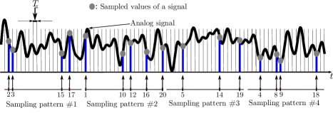
An example of a random sampling pattern is shown in Fig. 1.

2.2 Random patterns generation problem

Let us denote a nontrivial problem $\mathcal{P}(N,\tau,T_{\text{g}},f_{\text{s}}^{\dagger},t_{\text{min}},t_{\text{max}})$ of generation of a multiset (bag) $\mathbb{A}$ with $N$ random sampling patterns. The time length of sampling patterns is $\tau$, grid period is $T_{\text{g}}$. The requested average sampling frequency of patterns is $f_{\text{s}}^{\dagger}$, minimum and maximum intervals between sampling points are $t_{\text{min}}$ and $t_{\text{max}}$ respectively. The problem $\mathcal{P}$ is solved by random sampling pattern generators. The generators should meet requirements given in 2.4, and all the produced sampling patterns must meet the requirements given below in 2.3.

2.3 Requirements for random sampling patterns

2.3.1 Frequency stability

A random sampling pattern generator must produce sampling patterns with a requested average sampling frequency $f_{\textbf{s}}^{\dagger}$. If the average sampling frequency $f_{\textbf{s}}$ is lower than the requested sampling frequency, then the quality of signal reconstruction may be compromised. On the contrary, higher sampling frequency $f_{\textbf{s}}$ than the requested $f_{\textbf{s}}^{\dagger}$ causes unnecessary power consumption.

2.3.2 Minimum and maximum time intervals

A requirement for minimum interval $t_{\text{min}}$ between sampling points comes from the ADC technological constraints [9, 10, 4, 11]. Violation of this requirement may render the sampling pattern impossible to implement with a given ADC. Similarly, there may be a requirement of maximum interval between samples $t_{\text{max}}$. Generating an adequate random sampling pattern is realizable if $t_{\text{min}}\leq T_{\textbf{s}}^{\dagger}$ and $t_{\text{max}}\geq T_{\textbf{s}}^{\dagger}$, where $T_{\textbf{s}}^{\dagger}=1/f^{\dagger}_{\textbf{s}}$ is the requested average sampling period.

2.3.3 Unique sampling points

As stated in (2), sampling points in a given sampling pattern $\mathbb{T}$ cannot be repeated. Repeated sampling points do not make practical sense since a signal can be sampled only once in a given time moment. If a sampling pattern contains repeated sampling points, then a dedicated routine must remove these repeated points.

2.4 Requirements for random sampling pattern generators

2.4.1 Uniform probability density function for grid points

As described in 2.1, a sampling pattern $\mathbb{T}$ is an ordered set which is a subset of a grid $\mathbb{G}$. In other words, sampling points are drawn from a pool of grid points. The sampling pattern generator should not favor any of the sampling grid points. Ideally, all of the sampling points should be equi-probable.

2.4.2 Pattern uniqueness

Repeated sampling patterns generate unnecessary processing overhead, especially if sampling patterns are generated offline and further processed (Fig. 5). An additional search routine which removes replicas of sampling patterns must be implemented in this case. Therefore, the ideal random sampling pattern generator should not repeat sampling patterns unless all the possible sampling patterns have been generated.

3 Statistical evaluation of random sampling pattern generators

In this Section we propose statistical parameters for evaluation of a tested random sampling pattern generator. Aim of these parameters is to assess how well sampling patterns produced by the evaluated generator cope with the requirements described in 2.3 and 2.4. These parameters are to be computed for a bag $\mathbb{A}$ of $N$ patterns produced by the evaluated generator, the parameters are computed using the Monte Carlo method. It is checked if every generated sampling pattern fulfills requirements given in 2.3 and if a generated bag (multiset) of sampling patterns fulfill requirements given in the 2.4. According to our best knowledge, similar statistical evaluation has never been introduced before.

3.1 Frequency stability error parameters

Let us introduce a statistical parameter indicating how well the evaluated generator fulfills the imposed requirement of the requested average sampling frequency $f_{\text{s}}^{\dagger}$ (2.1):

$$e_{\text{f}}=\\ \frac{1}{N}\sum_{n=1}^{N}{\left(\frac{f^{\dagger}_{\text{s}}-f^{(n)}_{\text{s}}}{f^{\dagger}_{\text{s}}}\right)^{2}}=\\ \frac{1}{N}\sum_{n=1}^{N}{\left(\frac{K_{\text{s}}^{\dagger}-K_{\text{s}}^{(n)}}{K_{\text{s}}^{\dagger}}\right)^{2}}$$ (9)

where $f_{\text{s}}^{(n)}$ is the average sampling frequency of the $n$-th sampling pattern. Since all the sampling patterns have the same time length $\tau$, in practice it is usually more convenient to use the requested number of sampling points in a pattern $K_{\text{s}}^{\dagger}$ and count the number of actual sampling points in a pattern $K_{\text{s}}^{(n)}$. This parameter is an average value of a relative frequency error of every sampling pattern. The lower the parameter $e_{\text{f}}$ is, the better is the frequency stability of the generator. Additionally, let us introduce a $\gamma_{\text{f}}$ parameter:

$$\gamma_{\text{f}}=\frac{1}{N}\sum_{n=1}^{N}{\gamma^{(n)}_{\text{f}}}\quad\quad\gamma^{(n)}_{\text{f}}=\begin{cases}0&\text{for $K^{\dagger}_{\text{s}}=K^{(n)}_{\text{s}}$}\\ 1&\text{for $K^{\dagger}_{\text{s}}\neq K^{(n)}_{\text{s}}$}\\ \end{cases}$$ (10)

which is the ratio of patterns in a bag $\mathbb{A}$ which violate the frequency stability requirement. The parameter $\gamma^{(n)}_{\text{f}}=1$ denotes whether the average sampling frequency of the $n$-th pattern is incorrect.

3.2 Sampling point interval error parameters

Let us introduce statistical parameters which indicate how well the assessed generator meets the interval requirements discussed in Sec. 2.3.2. For a given $n$-th sampling pattern $\mathbb{T}^{(n)}$ let us create ordered subsets $\mathbb{D}^{(n)}_{-}\subset\mathbb{D}^{(n)}$ and $\mathbb{D}_{+}^{(n)}\subset\mathbb{D}^{(n)}$, where $\mathbb{D}$ is a set with intervals between sampling points as in (6). These subsets contain intervals between samples which violate the minimum and the maximum requirements between sampling points $t_{\text{min}}$ and $t_{\text{max}}$ respectively:

$$\mathbb{D}_{-}=\{d_{-,k}\in\mathbb{D}:d_{-,k}<t_{\text{min}}\}$$ (11)

$$\mathbb{D}_{+}=\{d_{+,k}\in\mathbb{D}:d_{+,k}>t_{\text{max}}\}$$ (12)

Now let us introduce statistical parameters $e_{\text{min}}$ and $e_{\text{max}}$:

$$e_{\text{min}}=\frac{1}{N}\sum_{n=1}^{N}{(e_{-}^{(n)})^{2}}\quad\quad e_{-}^{(n)}=\frac{|\mathbb{D}^{(n)}_{-}|}{|\mathbb{D}^{(n)}|}$$ (13)

$$e_{\text{max}}=\frac{1}{N}\sum_{n=1}^{N}{(e_{+}^{(n)})^{2}}\quad\quad e_{+}^{(n)}=\frac{|\mathbb{D}^{(n)}_{+}|}{|\mathbb{D}^{(n)}|}$$ (14)

where $|\cdot|$ denotes the number of elements in a set (set’s cardinality), and $|\mathbb{D}^{(n)}|=K_{\text{s}}-1$ as in (6). These parameters contain the average squared ratio of the number of intervals in a pattern which violate minimum/maximum interval requirements to the number of all intervals between sampling points in a pattern. The lower the above parameters are, the better the evaluated generator meets interval requirements. Similarly to the frequency stability parameter, let us introduce $\gamma_{\text{min}}$ and $\gamma_{\text{max}}$ parameters:

$$\gamma_{\text{min}}=\frac{1}{N}\sum_{n=1}^{N}{\gamma_{\text{min}}^{(n)}}\quad\quad\\ \gamma_{\text{min}}^{(n)}=\begin{cases}0&\text{for $|\mathbb{D}^{(n)}_{-}|=0$}\\ 1&\text{for $|\mathbb{D}^{(n)}_{-}|>0$}\\ \end{cases}$$ (15)

$$\gamma_{\text{max}}=\frac{1}{N}\sum_{n=1}^{N}{\gamma_{\text{max}}^{(n)}}\quad\quad\\ \gamma_{\text{max}}^{(n)}=\begin{cases}0&\text{for $|\mathbb{D}^{(n)}_{+}|=0$}\\ 1&\text{for $|\mathbb{D}^{(n)}_{+}|>0$}\\ \end{cases}$$ (16)

which are additional parameters which are equal to ratios of patterns which violate minimum or maximum intervals between sampling patterns. Parameters $\gamma_{\text{min}}^{(n)}=1$ and $\gamma_{\text{max}}^{(n)}=1$ denote if the $n$-th pattern meets the requirement of minimum and maximum intervals respectively.

3.3 Ratio of incorrect patterns

It is possible to assign to every $n$-th pattern a parameter $\gamma^{(n)}$ which denotes if a pattern violates the frequency stability (2.3.1) or the interval requirements (2.3.2). The ratio of incorrect patterns $\gamma$ of a bag $\mathbb{A}$ is:

$$\gamma=\frac{1}{N}\sum_{n=1}^{N}{\gamma^{(n)}}\quad\quad\gamma^{(n)}=\gamma^{(n)}_{\text{f}}\;\vee\;\gamma^{(n)}_{\text{min}}\;\vee\;\gamma^{(n)}_{\text{max}}$$ (17)

where $\vee$ is a logical disjunction. Using parameter $\gamma^{(n)}$ it is possible to generate a sub-bag $\mathbb{A}^{\star}\sqsubseteq\mathbb{A}$ which contains only correct patterns from the bag $\mathbb{A}$:

$$\mathbb{A}^{\star}=\{\mathbb{T}\;\;\textbf{in}\;\;\mathbb{A}:\;\;\gamma^{(n)}=0\}$$ (18)

where $\mathbb{T}\;\;\textbf{in}\;\;\mathbb{A}$ signifies that a pattern $\mathbb{T}$ is an element of a multiset $\mathbb{A}$. Please note that $\mathbb{A}$ is a multiset, so patterns which are the elements of $\mathbb{A}$ may be repeated, and patterns which are the elements of the multiset $\mathbb{A}^{\star}$ may also be repeated. Ideally, a sub-bag with correct patterns $\mathbb{A}^{\star}$ is identical to the original bag $\mathbb{A}$.

3.4 Quality parameter: Probability density function

Let us introduce a statistical parameter $e_{\text{p}}$ which indicates whether the probability density of occurrence for grid points in patterns from bag $\mathbb{A}$ is uniformly distributed:

$$e_{\text{p}}=\frac{1}{K_{\text{g}}}\sum_{m=1}^{K_{\text{g}}}{(p_{\text{g}}(m)-1)^{2}}$$ (19)

The probability of occurrence of the $m$-th grid point $p_{\text{g}}(m)$ is:

$$p_{\text{g}}(m)=\frac{K_{\text{g}}}{K_{\text{t}}}\sum_{n=1}^{N}{\text{g}_{m}(n)}\quad\quad K_{\text{t}}=\sum^{N}_{n}K_{\text{s}}^{(n)}$$ (20)

where $K_{\text{g}}$ is the number of sampling grid points in a sampling pattern, $K_{\text{t}}$ is the total number of sampling points in all the patterns in a bag $\mathbb{A}$, and the parameter $\text{g}_{m}(n)$ indicates whether the $m$-th grid point is used in the $n$-th sampling pattern $\mathbb{T}^{(n)}$:

$$\text{g}_{m}(n)=\\ \begin{cases}0&\text{if }mT_{\text{g}}\notin\mathbb{T}^{(n)}\\ 1&\text{if }mT_{\text{g}}\in\mathbb{T}^{(n)}\end{cases}$$ (21)

Additionally, let us introduce a statistical parameter $e_{\text{p}}^{\star}$ which is calculated identically to $e_{\text{p}}$, but based on sampling patterns from subbag $\mathbb{A}^{\star}$ (18).

3.5 Quality parameter: Uniqueness of patterns

Let us create a set $\mathbb{A}_{\#}$ for a bag $\mathbb{A}$ of $N$ sampling patterns generated by the evaluated pattern generator which contains only unique patterns from $\mathbb{A}$. Similarly, let us create a set $\mathbb{A}_{\#}^{\star}$ which contains only unique patterns from the subbag with correct patterns $\mathbb{A}^{\star}$ (18). Now let us introduce parameters $\eta_{N}$ and $\eta^{\star}_{N}$:

$$\eta_{N}=|\mathbb{A}_{\#}|\quad\quad\eta^{\star}_{N}=|\mathbb{A}^{\star}_{\#}|$$ (22)

These parameters count the number of unique patterns and unique correct patterns in the bag $\mathbb{A}$ with $N$ generated patterns.

4 Pattern generators

Algorithms of sampling pattern generators are presented in this Section. Subsection 4.1 presents existed, widely known Jittered Sampling (JS) and Additive Random Sampling (ARS) algorithms. Subsection 4.2 presents the proposed sampling pattern generator algorithm, which is tailored to fulfill the requirements presented in 2.3 and 2.4. Please note that all the algorithms presented in this paper generate sampling patterns represented as indices of sampling grid points as in (5).

4.1 Jittered Sampling and Additive Random Sampling

Jittered Sampling and Additive Random Sampling algorithms are widely used to generate random sequences. There are 4 input variables to the JS and ARS algorithms: requested time of a sampling pattern $\tau$, grid period $T_{\text{g}}$, requested average sampling frequency $f^{\dagger}_{\text{s}}$ and the variance parameter $\sigma^{2}$. The realizable time of a sampling pattern $\hat{\tau}$ may differ from the given requested time of a pattern $\tau$ if the given time is not a multiple of the given grid period $T_{\text{g}}$. Before either of the algorithms is started, the number of grid points $K_{\text{g}}$ in a sampling pattern, the realizable time of a sampling pattern $\hat{\tau}$ and the realizable requested number of sampling points $\hat{K}^{\dagger}_{\text{s}}$ must be computed:

$$K_{\text{g}}=\left\lfloor\frac{\tau}{T_{\text{g}}}\right\rfloor\quad\quad\hat{\tau}=K_{\text{g}}T_{\text{g}}\quad\quad\hat{K}^{\dagger}_{\text{s}}=[\hat{\tau}f^{\dagger}_{\text{s}}]$$ (23)

where $[\cdot]$ signifies the rounding function, which returns an integer which is closest to the function’s argument. Because the algorithms operate on a discrete set of grid points, the realizable requested average sampling frequency $\hat{f}^{\dagger}_{\text{s}}$ may differ from the requested sampling frequency $f^{\dagger}_{\text{s}}$. The realizable requested average sampling frequency $\hat{f}^{\dagger}_{\text{s}}$ and realizable requested average sampling period $\hat{T}^{\dagger}_{\text{s}}$ is computed:

$$\hat{f}^{\dagger}_{\text{s}}=\frac{\hat{K}^{\dagger}_{\text{s}}}{\hat{\tau}}\quad\quad\hat{T}^{\dagger}_{\text{s}}=\frac{1}{\hat{f}^{\dagger}_{\text{s}}}\quad\quad\hat{N}^{\dagger}_{\text{s}}=\left[\frac{\hat{T}^{\dagger}_{\text{s}}}{T_{\text{g}}}\right]$$ (24)

where $\hat{N}^{\dagger}_{\text{s}}$ is the requested average sampling period recalculated to the number of grid periods. If the computed realizable requested sampling frequency $\hat{f}^{\dagger}_{\text{s}}$ is different from the requested sampling frequency $f^{\dagger}_{\text{s}}$, the problem of generation of sampling patterns is not well stated. Before the algorithms start, the index of a correct sampling point $\hat{k}$ and the starting position of the sampling point $n_{0}$ must be reset:

$$\hat{k}=0\quad n_{0}=0$$ (25)

In the JS algorithm, every sampling point is a uniform sampling point which is randomly ”jittered”:

$$n_{\mathrm{JS},k}^{\ast}=[k\hat{N}^{\dagger}_{\text{s}}+\sqrt{\sigma^{2}}x_{k}\hat{N}^{\dagger}_{\text{s}}]\quad x_{k}\thicksim\mathcal{N}(0,1)$$ (26)

where $\mathcal{N}(0,1)$ denotes a standard normal distribution. In the ARS algorithm every sampling point is computed using the previous sampling point to which an average sampling period and a random value are added:

$$n_{\mathrm{ARS},k}^{\ast}=[n_{\hat{k}-1}+\hat{N}^{\dagger}_{\text{s}}+\sqrt{\sigma^{2}}x_{k}\hat{N}^{\dagger}_{\text{s}}]\quad x_{k}\thicksim\mathcal{N}(0,1)$$ (27)

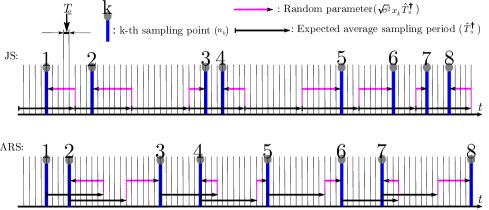
Fig. 4 illustrates generation of sampling patterns in the JS and ARS algoritms.

The practical versions of both JS and ARS algorithms are presented in Alg. 1. After generation of a pattern, any repeated sampling point must be removed (line 12 of Alg. 1). It is because in these algorithms there is no guarantee that sampling points are not repeated.

Algorithm 1 JS and ARS algorithms - pseudo code

1:  function $[\bm{\mathbb{T}}]=\mbox{\tt{JS/ARS}}(\bm{\tau},\bm{T_{\text{g}}},\bm{f_{\text{s}}^{\dagger}},\bm{\sigma^{2}})$

2:  Compute $K_{\text{g}}$, $\hat{\tau}$ and $\hat{K}^{\dagger}_{\text{s}}$ as in (23)

3:  Compute $\hat{f}^{\dagger}_{\text{s}}$, $\hat{T}^{\dagger}_{\text{s}}$ and $\hat{N}^{\dagger}_{\text{s}}$ as in (24)

4:  Reset $\hat{k}$ and $n_{0}$ as in (25)

5:  FOR $k=1$ TO $\hat{K}^{\dagger}_{\text{s}}$

6:      Draw sampling moment $n_{\mathrm{JS},k}^{\ast}$ (26) or $n_{\mathrm{ARS},k}^{\ast}$ (27)

7:      IF $n_{k}^{\ast}>0$ AND $n_{k}^{\ast}<\hat{\tau}$

8:          $n_{\hat{k}}\leftarrow n_{\hat{k}}^{\ast}$

9:          Assign $\mathbb{T}^{\prime}(\hat{k})\leftarrow n_{\hat{k}}$

10:          $\hat{k}\leftarrow\hat{k}+1$

11:  END

12:  Remove repeated sampling points in $\mathbb{T}$

4.2 ’ANGIE’ algorithm

We propose an algorithm which would perfectly cope with the requirements described in 2.3 and as much as possible with the requirements in 2.4. The ratio of incorrect patterns $\gamma$ (17) generated by the algorithm should always equal 0, while keeping the probability density parameter $e_{\text{p}}$ (Sec. 3.4) as low as possible and the uniqueness parameter $\eta_{N}=\eta_{N}^{\star}$ (Sec. 3.5) as high as possible. The parameters $e^{\star}_{\text{p}}$ and $\eta_{N}^{\star}$ must equal $e_{\text{p}}$ and $\eta_{N}$ respectively, as the subbag with correct patterns $\mathbb{A}^{\star}$ must be identical to the subbag with all the patterns $\mathbb{A}$ (all the generated patterns must be correct). Therefore we propose the rANdom sampling Generator with Intervals Enabled (ANGIE) algorithm. The input variables to the algorithm are identical to the JS and ARS algorithms (4.1), with additional variables for the allowed time between samples ($t_{\text{min}}$, $t_{\text{max}}$).

Before the ANGIE algorithm starts, the following precomputations must be done. Similarly to the JS and ARS algorithms, the number of grid points in a sampling pattern ($K_{\text{g}}$), the realizable time of a sampling pattern ($\hat{\tau}$) and the realizable number of sampling points in a sampling pattern $\hat{K}^{\dagger}_{\text{s}}$ must be computed as in (23). Then the minimum and the maximum time between sampling points must be recalculated to the number of grid points:

$$K_{\text{min}}=\left\lceil\frac{t_{\text{min}}}{T_{\text{g}}}\right\rceil\quad K_{\text{max}}=\left\lfloor\frac{t_{\text{max}}}{T_{\text{g}}}\right\rfloor$$ (28)

where $\left\lceil\cdot\right\rceil$ signifies the ceiling function which returns the lowest integer which is higher or equal to the function’s argument. In the proposed algorithm there are 2 limit variables, $n_{k}^{-}$ and $n_{k}^{+}$, which are the first and the last possible position of a $k$-th sampling point. These variables are updated after generation of every sampling point. Before the algorithm starts these variables must be initialized:

$$n_{1}^{-}=1\quad\quad n_{1}^{+}=K_{\text{g}}-K_{\text{min}}(\hat{K}^{\dagger}_{\text{s}}-1)$$ (29)

The number of sampling points left to be generated is updated before generation of every sampling point:

$$n_{k}^{\text{left}}=\hat{K}^{\dagger}_{\text{s}}-k+1$$ (30)

where $k$ is the index of the current sampling point. The average sampling period for the remaining $n_{k}^{\text{left}}$ sampling points and the expected position $e_{k}$ of the $k$-th sampling point is:

$$e_{k}=n_{k-1}+n_{k}^{\ddagger}\quad\quad n_{k}^{\ddagger}=\left[\frac{K_{\text{g}}-n_{k-1}}{n_{k}^{\text{left}}+1}\right]$$ (31)

In the proposed algorithm, a $k$-th sampling point $n_{k}$ may differ from its expected position $e_{k}$ by the interval $n_{k}^{\text{d}}$. Before computing this interval the algorithm must compute intervals to the limits:

$$n_{k}^{\text{d}-}=|e_{k}-n_{k}^{-}|\quad\quad n_{k}^{\text{d}+}=|n_{k}^{+}-e_{k}|$$ (32)

and then the lower from the above intervals is the correct interval $n_{k}^{\text{d}}$:

$$n_{k}^{\text{d}}=\min{(n_{k}^{\text{d}-},n_{k}^{\text{d}+})}$$ (33)

The first sampling point is drawn using a uniformly distributed variable $x^{u}$:

$$n_{1}=\lceil x_{1}^{u}n_{k}^{\ddagger}\rceil\quad x_{1}^{u}\thicksim\mathcal{U}(0,1)$$ (34)

while the rest of the sampling points are drawn using the normal distribution:

$$n_{k}=e_{k}+[x_{k}n_{k}^{\text{d}}]\quad x_{k}\thicksim\mathcal{N}(0,\sigma^{2})$$ (35)

Finally, the algorithm checks whether the drawn sampling moment $n_{k}$ violates the limits $n_{k}^{-}$ and $n_{k}^{+}$:

$$n_{k}=\begin{cases}n^{+}_{k}&\text{for $n_{k}>n^{+}_{k}$}\\ n^{-}_{k}&\text{for $n_{k}<n^{-}_{k}$}\\ \end{cases}$$ (36)

In the last step the limits for the next sampling point are computed. The lower and the higher limits are computed as:

$$n_{k+1}^{-}=n_{k}+K_{\text{min}}\quad\quad n_{k+1}^{+}=K_{\text{g}}-K_{\text{min}}(n_{k}^{\text{left}}-2)$$ (37)

If the maximum time between samples is valid ($t_{\text{max}}<\inf$), then the higher limit should be additionally checked for $t_{\text{max}}$:

$$n_{k+1}^{+}=\min{({n_{k+1}^{+},n_{k}+K_{\text{max}}})}$$ (38)

The proposed algorithm is presented in Alg. 2.

Algorithm 2 ’ANGIE’ algorithm - pseudo code

1:  function $[\bm{\mathbb{T}}]=\mbox{\tt{ANGIE}}(\bm{\tau},\bm{T_{\text{g}}},\bm{f_{\text{s}}^{\dagger}},\bm{t_{\text{min}}},\bm{t_{\text{max}}},\bm{\sigma^{2}})$

2:  Compute $K_{\text{g}}$, $\hat{\tau}$ and $\hat{K}^{\dagger}_{\text{s}}$ as in (23)

3:  Compute $K_{\text{min}}$ and $K_{\text{max}}$ as in (28)

4:  Initialized the limits $n_{1}^{-}$ and $n_{1}^{+}$ as in (29)

5:  FOR $k=1$ TO $\hat{K}^{\dagger}_{\text{s}}$

6:      Update the number of sampling points left $n^{\text{left}}_{k}$ as in (30)

7:      Compute the expected position $e_{k}$ as in (31)

8:      Compute the interval $n_{k}^{\text{d}}$ as in (33)

9:      Draw sampling moment $n_{k}$ as in (34) or (35)

10:      Check and correct $n_{k}$ as in (36)

11:      Assign $\mathbb{T}^{\prime}(k)\leftarrow n_{k}$

12:      Update the limits $n_{k+1}^{-}$ and $n_{k+1}^{+}$ as in (37) and (38)

13:  END

5 Numerical experiment

In this section, the performance of the proposed ANGIE algorithm is experimentally compared with the JS and ARS algorithms. A toolbox with pattern generators and evaluation functions was created to facilitate the experiment. Emphasis was set on validation of parts of the software. The toolbox, together with its documentation, is available online at [21]. Using the content available at [21] it is possible to reproduce the presented numerical simulations.

5.1 Experiment #1 - setup

The duration $\tau$ of sampling patterns is set to 1 ms, sampling grid period $T_{\text{g}}$ is equal to 1 $\mu$s. The requested average sampling frequency of patterns is set to 100 kHz, which corresponds to an average sampling period equal to 10 $\mu$s. The minimum time between sampling points is $t_{\text{min}}=5\mu$s, and there is no requirement for maximum time between sampling points ($t_{\text{max}}=\inf$). The variance $\sigma^{2}$ is logarithmically swept in the range $[10^{-4},10^{2}]$.

The computed statistical parameters of sampling patterns are automatically tested for convergence. A mean value is accounted as converged, if for the last $2\cdot 10^{4}$ patterns it did not change more than 1% of the mean value computed for all the patterns currently tested. The minimum number of sampling patterns tested is $10^{5}$. The uniqueness parameters $\eta_{N}$ and $\eta_{N}^{\star}$ (22) are computed after $N=10^{5}$ patterns.

5.2 Experiment #1 - results

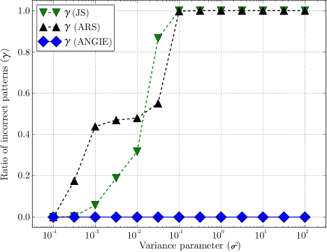
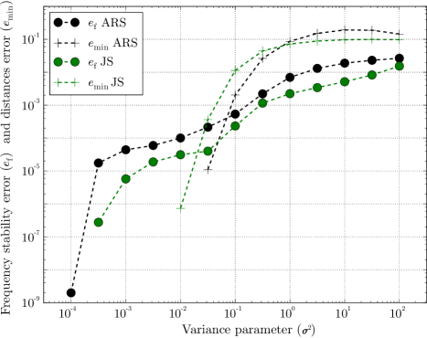
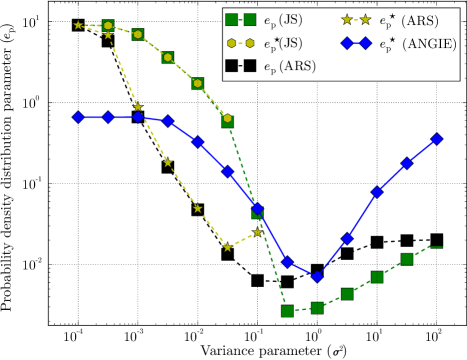
Error parameters computed for the tested sampling pattern generators are plotted in Fig. 7. The ratio of incorrect patterns are plotted in Fig. 6. This ratio for the ANGIE algorithm (blue $\diamond$) is equal to 0 for all the values of variance $\sigma^{2}$. Thus, all the pattens have correct average sampling frequency and intervals between sampling points. Patterns generated by the JS (green $\blacktriangledown$) and the ARS algorithms (black $\blacktriangle$) are all correct for very low values of the variance $\sigma^{2}$, but the quality parameters $e_{\text{p}}$ and $\eta_{10^{5}}$ for these $\sigma^{2}$ values are poor (Fig. 8 and Fig. 9). In Fig. 7 it can be seen that for nearly all the values of variance $\sigma$, the frequency stability of the patterns generated by the JS and the ARS algorithms is compromised, and for most of the values of $\sigma^{2}$, the requirement of minimum intervals between sampling points is not met by these algorithms.

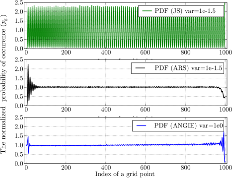
The best values of the parameter $e_{\text{p}}$ are achieved for the JS (green $\blacksquare$) and the ARS (black $\blacksquare$) algorithms (Fig. 8), but only if all the patterns (also incorrect) are taken into account (parameter $e_{\text{p}}$). If the quality parameter was computed only for the correct patterns (parameter $e_{\text{p}}^{\star}$), it can be clearly seen that the proposed algorithm (blue $\blacksquare$) performs significantly better than the JS (yellow $\hexagon$) and the ARS algorithms (yellow $\star$). Furthermore, the best values of $e_{\text{p}}^{\star}$ are found for the values of variance $\sigma$ for which most of the patterns produced by the JS and the ARS algorithms are incorrect. Plots of the best probability density functions found for the tested algorithms are in Fig. 10.

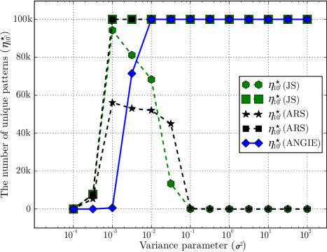
Fig. 9 shows the number of unique patterns produced by the tested algorithms. The number of unique correct patterns produced by the proposed algorithm is higher than the number produced by the JS and the ARS algorithms for any variance value $\sigma^{2}\geq 10^{-2}$.

The above results show that the proposed algorithm ANGIE performs better than the JS and the ARS algorithms. All the patterns generated by the ANGIE algorithm are correct, have a parameter $\gamma^{(n)}$ defined as in (17) equal to 0. The quality parameters described in Sec. 3.4 and Sec. 3.5 are better for the proposed algorithm. It can be seen that the variance value $\sigma^{2}$, which is an internal algorithm parameter, should be adjusted to a given problem. For the given problem, the proposed algorithm performs best for $\sigma^{2}=10^{-2}$.

5.3 Experiment #2 - setup

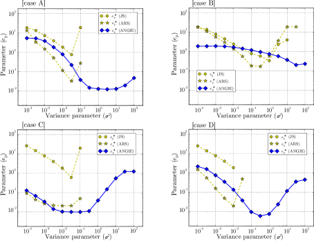
In the second experiment four different cases (A-D) of sampling patterns are studied. Parameters of these cases are collected in Table 1. In the first two cases there are requirements of both the minimum and the maximum distance between sampling points. In the second case there are only 5 sampling points requested p. sampling pattern, and the number of sampling grid points is limited to 100. In the third case there are no requirements imposed on distances between sampling points, so there is only the requirement of stable average sampling frequency. This case is distinctive from others, because the number of sampling points p. sampling pattern is high ($10^{4}$), and the grid period is very low. In the last case there is a requirement of the maximum distance between sampling points. In all the four cases the variance $\sigma^{2}$ is logarithmically swept in the range $[10^{-4},10^{2}]$.

In this experiment there are three quality parameters measured for all the three generators (JS, ARS and ANGIE). The first parameter is the ratio of incorrect patterns $\gamma$ (17). The second is the probability density parameter $e_{\text{p}}^{\star}$ as in (19), but computed only for the correct patterns. The third quality parameter is the number of unique correct patterns in the first $10^{4}$ generated patterns $\eta^{\star}_{10^{4}}$ (22).

	Independent parameters					Dependent parameters
	$\tau$	$T_{g}$	$f_{s}$	$t_{\text{min}}$	$t_{\text{max}}$	$K_{g}$	$\hat{K}^{\dagger}_{\text{s}}$	$K_{\text{min}}$	$K_{\text{max}}$
case	[ms]	[$\mu$s]	[kHz]	[ms]	[ms]
A	$10^{3}$	$10^{3}$	0.05	10	30	$10^{3}$	50	10	30
B	0.1	1	50	0.015	0.028	100	5	15	28
C	$10^{3}$	1	10	—	—	$10^{6}$	$10^{4}$	—	—
D	0.005	25$\cdot$ $10^{-5}$	$10^{5}$	—	14$\cdot 10^{-6}$	2$\cdot$ $10^{4}$	500	—	56

Table 1: Parameters of sampling patterns used in all the four cases of experiment #2. Independend parameters are: time length of sampling patterns ($\tau$), grid period ($T_{g}$), requested average sampling frequency ($f_{s}$), minimum allowed time between sampling points ($t_{\text{min}}$), maximum allowed time between sampling points ($t_{\text{max}}$). Shown dependent parameters are: the number of grid points ($K_{g}$), the requested realizable number of sampling points ($\hat{K}^{\dagger}_{\text{s}}$), the minimum and maximum time between the sampling points recalculated to the number of grid points ($K_{\text{min}}$ and $K_{\text{max}}$).

5.4 Experiment #2 - results

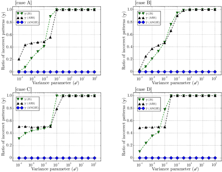
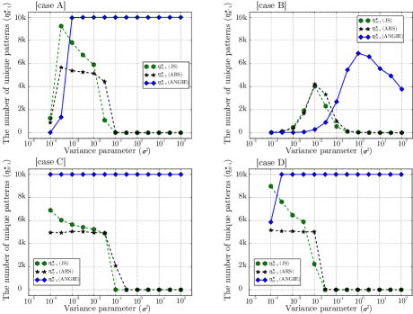
Results of this experiment are shown on Figures 11–13. Each Figure presents a measured quality parameter for all the four cases. The ratio of incorrect patterns $\gamma$ is on Fig. 11, the probability density parameter $e_{\text{p}}^{\star}$ is on Fig. 12, and the number of unique correct patterns $\eta^{\star}_{10^{4}}$ is on Fig. 13.

Let us take a look at the ratio of incorrect patterns (Fig. 11). The ANGIE algorithm generates only correct sampling patterns. Hence to line 10 in the algorithm (see Algorithm 2), the minimum and the maximum distances between sampling points are kept. Lines 6–8 in the ANGIE algorithm ensure that there will be place for the correct number of sampling points in all the generated sampling patterns. To the contrary, both ARS and JS algorithms generate a lot of incorrect patterns. For the high values of variance $\sigma^{2}$ there are only incorrect patterns generated by these two algorithms.

In the three cases (A, C, D) the best probability density parameter $e_{\text{p}}^{\star}$ (Fig. 12) measured for patterns generated by the ANGIE algorithm is better than for the other two algorithms. Additionally, it can be seen in Fig. 13 that the generated number of unique correct sampling patterns is in all the four cases significantly higher for the proposed ANGIE algorithm. Let us take a closer look on the case B. In this case, the best probability density parameter $e_{\text{p}}^{\star}$ found for the algorithm ARS ($\sigma^{2}=10^{-0.5}$) is slightly better than the best $e_{\text{p}}^{\star}$ found for the ANGIE ($\sigma^{2}=10^{1.5}$). Still, the number of unique patterns is significantly better for the above values of $\sigma^{2}$ for ANGIE algorithm, and very most of the patterns generated by the ARS are incorrect for $\sigma^{2}=10^{-0.5}$.

We tried to find a case for which ARS and JS algorithms would clearly and distinctly outperform the ANGIE, but it turned out to be an impossible task. Still though, it is difficult to provide the reader with one gold rule which algorithm should be used. In practical applications there may be a huge number of different sampling scenarios, in this paper we covered only a tiny fraction of examples, and therefore every case should be considered separately. In general, ANGIE algorithm will always generate correct sampling patterns. But if these sampling patterns will have all quality parameters (especially $e_{\text{p}}^{\star}$) better than sampling patterns generated by the other algorithms, that is an another issue. From our experience we claim that indeed, in most of the cases ANGIE is the right choice. However, there might be applications in which, for example, equi-probability of occurrence of every sampling point is a critical matter and other algorithms might perform better. In practical applications, a numerical experiment should be always conducted to choose a correct pattern generator and to adjust variance value $\sigma^{2}$.

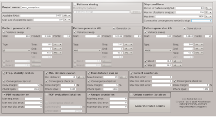
We prepared a software PAtterns TEsting System (PATES), which is open-source and available online [21]. This software contains all the three generators considered in this paper plus routines which compute the proposed quality parameters. With this software a user is able to test the generators for his own sampling scenario. We have created a graphical user interface to the software (Fig. 14), which makes using the system more intuitive. Reproducible research scripts which can be used to produce results from the presented experiments are also available in [21].

6 Implementation issues

In this Section we discuss some of the implementation issues of random sampling patterns. In this paper, we focus on offline sampling pattern generation (Fig. 5), where patterns are prepared offline by a computational server and then stored in a memory which is a part of a signal processing system. Immediate generation of sampling patterns would require very fast pattern generators which are able to generate every sampling point in a time much shorter than minimum time between sampling points $t_{\text{min}}$. The ANGIE algorithm (Alg. 2) requires a number of floating point computations before every sampling point is computed, therefore very powerful computational circuit would be necessary in real time applications where $t_{\text{min}}<1\mu s$.

6.1 Software patterns generator

In practical applications there is a need to generate $N\gg 1$ sampling patterns. Sampling patterns are generated offline (Fig. 5) on a computational server. In naive implementation, Alg. 2 is repeated $N$ times to generate $N$ random sampling patterns. This approach is suboptimal, because computation of initial parameters from equations (23) and (28) (lines 2-3) is unnecessarily repeated $N$ times. In the optimal implementation lines 2-3 are performed only once before a bag of patterns is generated.

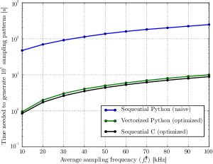
We implemented the ANGIE algorithm (naive implementation) in Python. Furthermore, we prepared an implementation in C and an optimized implementation in Python (vectorized code). All the implementations are available for download at [21]. Fig. 15 shows time needed to generate $N=10^{5}$ sampling patterns. Parameters of sampling patterns are identical to the parameters used in the experiment described in Section 5.1. The average sampling frequency is swept from 10 kHz to 100 kHz, and the duration of the patterns is kept fixed. Measurements were made on an Intel Core i5-3570K CPU, and a single core of the CPU was used.

The ANGIE algorithm operates mostly on integer numbers, and therefore it requires maximally only three floating point operations p. sampling point. The algorithm time complexity vs. the average sampling frequency of a pattern is $O(n)$ (consider the logarithmic vertical scale), because lines 5-13 in Alg. 2 are repeated for every sampling point which must be generated. As expected, the optimized vectorized Python / optimized C implementation is much faster than the naive Python implementation.

6.2 Driver of an analog-to-digital converter

The analog-to-digital converter (ADC) driver is a digital circuit which triggers the converter according to a given sampling pattern. The maximum clock frequency of the driver determines the minimum grid period. Detailed construction of the driver depends on the used ADC because the driver must generate specific signals which drive the ADC.

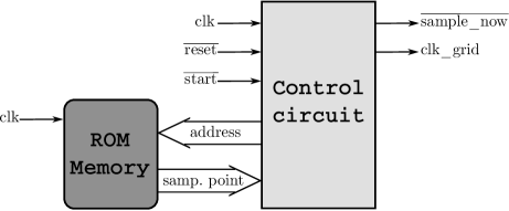
A simple driver marks the ’sample now’ signal every time the grid counter reaches a value equal to the current sampling time point. Such a driver was implemented in VHDL language. The structure of the driver is shown in Fig. 16. Due to the internal structure of the control circuit, the grid period is eight times longer then the input clock period. Table 2 contains results of synthesis of the driver in four different Xilinx FPGAs.

Xilinx	Max clock	Min grid
FPGA	frequency [MHz]	period $T_{\text{g}}$ [ns]
Spartan 3	439.97	18.2
Virtex 6	1078.98	7.4
Artix 7	944.47	8.5
Zynq 7020	1160.36	6.9

Table 2: Maximum clock values and minimum grid periods of an implemented driver in different Xilinx FPGAs

Sampling patterns are read from a ROM. The amount of memory $n_{\text{m}}$ used to store a sampling pattern [in bytes] is:

$$n_{\text{m}}=K_{\text{s}}\cdot\left\lceil\frac{\log_{2}{K_{\text{g}}}}{8}\right\rceil$$ (39)

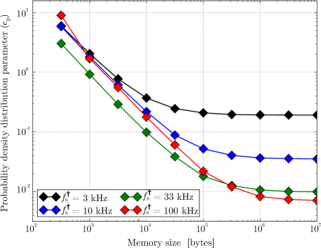
where $K_{\text{g}}$ is the number of grid points in a pattern and $K_{\text{s}}$ is the number of sampling points in a pattern. Depending on the available size of memory, different numbers of sampling patterns can be stored. Fig. 17 shows the relation between the memory size and the probability density parameter $e_{\text{p}}$ (19) computed for the proposed ANGIE algorithm. The parameters of the sampling patterns are identical to the parameters used in the experiment described in Section 5.1, although four different average sampling frequencies are used.

As expected, the higher the average sampling frequency of patterns, the better the distribution of probability density function (parameter $e_{\text{p}}$ is lower). The higher the average sampling frequency of patterns, the more the memory needed to achieve the best possible probability density parameter $e_{\text{p}}$. If the available memory is low, the probability density function becomes less equi-probable.

7 Conclusions

This paper discussed generation of random sampling patterns dedicated to event-driven ADCs. Constraints and requirements for random sampling patterns and pattern generators were discussed. Statistical parameters which evaluate sampling pattern generators were introduced. We proposed a new algorithm which generates constrained random sampling patterns. The patterns generated by the proposed algorithm were compared with patterns generated by the state-of-the-art algorithms (Jittered Sampling and Additive Random Sampling). It was shown, that the proposed algorithm performs better in generation of random sampling patterns dedicated to event-driven ADCs. Implementation issues of the proposed method were discussed.

References

- [1] H. S. Shapiro, R. A. Silverman, “Alias free sampling of Random Noise”, IEEE Trans. Info. Theory, vol. 16, pp. 147–152, (1960)
- [2] H. G. Feichtinger and K. Gröchenig and T. Strohmer, “Efficient Numerical Methods In Non-Uniform Sampling Theory”, Numerische Matematik, vol. 69, pp. 423–440, (1995)
- [3] I. Homjakovs, M. Greitans, R. Shavelis, “Real-Time Acquisitions of Wideband Signals Data Using Non-Uniform Sampling”, Proc. IEEE Eurocon 2009, pp. 1158–1163, Saint-Petersburg, May. 2009.
- [4] Hui-Qing Liu, “ADS82x ADC with non-uniform sampling clock.”, Analog Applications Journal, (2005)
- [5] M. Wakin, S. Becker, E. Nakamura, M. Grant, E. Sovero, D.Ching, J. Yoo, J. Romberg, A. Emami-Neyestanak, E. Candes, “A Nonuniform Sampler for Wideband Spectrally-Sparse Environments”, IEEE Trans. Emerg. Sel. Topics Circuits Syst. vol. 2(3), (2012)
- [6] E.J. Candès and M. B. Wakin, “An Introduction To Compressive Sampling”, IEEE Signal Process. Mag., vol. 25(2), pp. 21–30, (2008)
- [7] J. Laska, S. Kirolos, Y. Massoud, R. Baraniuk, A. Gilbert, M. Iwen and M. Strauss, “Random Sampling for Analog-to-Information Conversion of Wideband Signals”, Proc. IEEE Dallas Circuits and Systems Workshop (DCAS), pp. 119–122, Dallas, USA, (2006)
- [8] R.G. Baraniuk, M. Davenport, R. Devore, M. Wakin, “A Simple Proof of the Restricted Isometry Property for Random Matrices”, Constructive Approximation, vol. 28(3), pp. 253-263, (2008)
-
[9]
Analog Devices (2013).
“A/D Converters. Analog Devices.”,[Online] Available:
http://www.analog.com/en/analog-to-digital-converters/ad-converters/products/index.html - [10] B. Le, T. W. Rondeau, J. H. Reed, W. Bostian, “Analog-to-Digital Converters. A review of the past, present, and future.”, IEEE Sig. Proc. Mag., vol. 22(6), (2005)
[11]
Xilinx (2012).
“7 Series FPGAs and Zynq-7000 All Programmable SoC
XADC Dual 12-Bit 1 MSPS
Analog-to-Digital Converter”,[Online] Available:
http://www.xilinx.com/support/documentation/user_guides/ug480_7Series_XADC.pdf - [12] F. Marvasti, “Spectral analysis of irregular samples of mu1tidimensional signals,”, Presented the 6th Workshop on Multidim. Signal Processing, Pacific Grove, California, (sep. 1989)
- [13] A. C. Gilbert, M. J. Strauss, and J. A. Tropp, “A Tutorial on Fast Fourier Sampling”, IEEE Signal Process. Mag., vol. 25, pp. 57-66, (2008)
- [14] F. Marvasti, “Nonuniform Sampling, Theory and Practice”, Springer Science + Business Media, (2001), ISBN: 978-1-4613-5451-2, New York, USA
- [15] J.J. Wojtiuk, “Randomized Sampling for Radio Design”, PhD Thesis, University of Southern Australia, (2000)
- [16] Y. P. Lin, and P.P. Vaidyanathan, “Periodically Nonuniform Sampling of Bandpass Signals”, IEEE Trans. Circuits Syst. II, vol. 45(3), pp. 340–351, (1998)
- [17] I. Bilinskis, A. Mikelsons, “Randomized Signal Processing.”, Prentice Hall, (1992), ISBN: 978-0-137-51074-0, Cambridge, UK
- [18] F. Papenfuß, Y.Artyukh, E. Boole, D. Timmermann, “Nonuniform Sampling Driver Design For Optimal ADC Utilization”, Proc. Internal Symposium on Circuits and Systems, 2003 (ISCAS’03), vol. 4, pp. 516–519, Bangkok, Thailand, (2003)
- [19] M. Ben-Romdhane, C. Rebai, P. Desgreys, A. Ghazeli, P. Loumeau, “Pseudorandom Clock Signal Generation for Data Conversion in a Multistandard Receiver”, Proc. IEEE Int. Conference on Design and Technology of Integrated Systems in Nanoscale Era, pp. 1Ð-4, Tozeur, Tunisia, (2008)
- [20] P. Vandewalle, J. Kovacevic, and M. Vetterli, “Reproducible Research in Signal Processing [What, why and how]”, IEEE Signal Process. Mag., vol. 26(3), pp. 37–47, (2009)
[21]
Aalborg University (2013).
“IRfDUCS project”, [Online]
Available:
http://www.irfducs.org/pates/
Acknowledgment
The work is supported by The Danish Council for Independent Research under grant number 0602–02565B.