Best of Both Worlds: Uniform sampling in Cartesian and Cayley Molecular Assembly Configuration Space

Abstract

EASAL (efficient atlasing and sampling of assembly landscapes) is a recently reported geometric method for representing, visualizing, sampling and computing integrals over the potential energy landscape tailored for small molecular assemblies. EASAL’s efficiency arises from the fact that small assembly landscapes permit the use of so-called Cayley parameters (inter-atomic distances) for geometric representation and sampling of the assembly configuration space regions; this results in their isolation, convexification, customized sampling and systematic traversal using a comprehensive topological roadmap, ensuring reasonable coverage of crucial but narrow regions of low effective dimension.

However, this alone is inadequate for accurate computation of configurational entropy and other integrals, required for estimation of both free energy and kinetics - where it is essential to obtain uniform sampling in appropriate cartesian or moduli space parameterization. Standard adjustment of Cayley sampling via the Jacobian of the map between the two parameterizations is fraught with challenges stemming from an illconditioned Jacobian.

This paper formalizes and analyzes these challenges to provide modifications to EASAL that secure the advantages of Cayley sampling while ensuring certain minimum distance and coverage relationships between sampled configurations - in Cartesian space. The modified EASAL’s performance is compared with the basic EASAL and the data are presented for Human and Rat Islet Amylin Polypeptide (HiAPP, PDB-2KJ7 and RiAPP PDB-2KB8) dimerization (the two differ in only 6 out of 37 residues, but the former aggregates into fibrils, while the latter does not).

I Introduction

Understanding and engineering a variety of supramolecular assembly, packing and docking processes even for small assemblies requires a comprehensive atlasing of the topological roadmap of the constant-potential-energy regions, as well as the ability to isolate and sample such regions and their boundaries even if they are narrow and geometrically complex. A recently reported geometric method called EASAL (efficient atlasing and sampling of assembly landscapes) Ozkan2014MainEasal provides such comprehensive atlasing as well as customized and efficient sampling of its regions, crucially employing so-called Cayley or distance parameters. However, for developing hybrids that combine the complementary strengths of EASAL and prevailing methods that predict noncovalent binding affinities and kinetics, accurate computation of configurational entropy and other integrals is essential. This in turn requires uniform distribution over the cartesian or appropriate Cartesian space parametrization. Standard adjustments using the Jacobian of the Cartesian-Cayley map poses multiple challenges due to illconditioning. This paper analyzes these challenges and develops a modification of EASAL that combines the best of both worlds of Cayley sampling with uniform distribution in Cartesian space.

I.1 Recent Related Work

A number of very recent results are directly related to or build upon the approach presented here. First, the basic EASAL approach was first described in Ozkan2011 . The approach is discussed in detail in Ozkan2014MainEasal , which gives EASAL-based computations of entropy integrals for clusters of assembling spherical particles that both simplify and extend the methodology and computational results of Holmes-Cerfon2013 that were reported after Ozkan2011 appeared. A multi-perspective comparison of variants of EASAL including the modification described here with traditional Montecarlo sampling of the assembly landscape of 2 transmembrane helices is given in Ozkan2014MC with a view towards leveraging complementary strengths for hybrid methods. An application of EASAL towards detecting assembly-crucial inter-atomic interactions for viral capsid self-assembly is given in Wu2012 ; Wu2014Virus (applied to 3 viral systems - Minute virus of Mice (MVM), Adeno-associated virus (AAV), and Bromo-mosaic virus (BMV)). Finally the architecture and functionalities of an opensource software implementation of the basic EASAL is described in Ozkan2014TOMS .

I.2 Previous Work, Scope and Motivation

There has been a long and distinguished history of configurational entropy and free energy computation methods kaku ; Andricioaei_Karplus_2001 ; Hnizdo_Darian_Fedorowicz_Demchuk_Li_Singh_2007 ; Hnizdo_Tan_Killian_Gilson_2008 ; Hensen_Lange_Grubmuller_2010 ; Killian_Yundenfreund_Kravitz_Gilson_2007 ; Head_Given_Gilson_1997 ; GregoryS201199 ; doi:10.1021/jp2068123 , many of which use as input the configuration trajectories of Molecular Dynamics or Monte Carlo sampling which are known to be nonergodic, whereby locating and isolating narrow channels and their boundaries, i.e., regions of low effective dimension separated by high energy barriers might take arbitrarily long, requiring several trajectories starting from different initial configuations.

This also causes problems for many entropy computation methods that rely on principal component analyses of the covariance matrices from a trajectory of MC samples in internal coordinates, followed by a quasiharmonic Andricioaei_Karplus_2001 or nonparametric (such as nearest-neighbor-based) Hnizdo_Darian_Fedorowicz_Demchuk_Li_Singh_2007 estimates. Since MC trajectories are not geometrically optimized, these methods are generally known to overestimate the volumes of configuration space regions with high geometric or topological complexity, even when hybridized with higher order mutual information Hnizdo_Tan_Killian_Gilson_2008 , and nonlinear kernel methods, such as the Minimally Coupled Subspace approach of Hensen_Lange_Grubmuller_2010 . Most of the above methods do not explicitly restrict the number of atoms in each of the assembling rigid molecular components, and in fact they are used for assembly or folding. For cluster assemblies from spheres, (with $k\leq 12$), there are a number of methods Holmes-Cerfon2013 ; Hagen1993 ; Doye1996 ; Meng2010 ; Gazzillo2006 to compute free energy and configurational entropy for subregions of the configuration space, and some of these subregions are the entire configuration spaces of small molecules such as cyclo-octane Martin2010 ; Jaillet2011 ; Porta2007 . These include robotics and computational geometry based methods such as GregoryS201199 ($n=3$). These methods are used to give bounds or to approximate configurational entropy without relying on Monte Carlo or Molecular Dynamics sampling. Note that there is an extensive literature purely on computing minimum potential energy configurations: these are are not relevant to this paper; neither are simulation-based methods for free-energy computation of large assemblies starting from known free energy values and formation rates for assembly intermediates formed from a small number of subassemblies.

Essentially, even for small assemblies, barring a few exceptions such as Holmes-Cerfon2013 , Porta2007 , Yao_Sun_Huang_Bowman_Singh_Lesnick_Guibas_Pande_Carlsson_2009 , and Gfeller_DeLachapelle_DeLos_Rios_Caldarelli_Rao_2007 ; Varadhan_Kim_Krishnan_Manocha_2006 ; Lai_Su_Chen_Wang_2009 ; 10.1371/journal.pcbi.1000415 , most prevailing methods do not extract a high-level, topological roadmap of the boundary relationships between the constant-potential-energy regions. Similarly, most prevailing methods of sampling and volume computation are not explicitly tailored or specialized to leverage this relative geometric simplicity of constant-potential-energy regions of assembly configuration spaces.

Hence for small assemblies, the basic EASAL Ozkan2011 ; Ozkan2014MainEasal addresses the demand for a method that satisfies two criteria: it should (i) generate a comprehensive roadmap of the assembly configuration space as a topological complex of constant-potential-energy regions, their neighborhood relationships and boundaries; and (ii) explicitly formalize and leverage the geometric simplicity of these regions (in the case of assembly relative to folding) to give an efficient and accurate computation of their volume by isolation of the region and its boundaries and customized sampling. In order to effectively combine the complementary advantages of EASAL with the abovementioned prevailing methods, the goal of this paper is to maintain these advantages of EASAL and Cayley sampling while ensuring certain minimum distance and coverage relationships between sampled points in Cartesian space.

II Methodology

The first subsection gives background from Ozkan2011 ; Ozkan2014MainEasal for the theoretical underpinnings of EASAL’s key features - geometrization, stratification and convexification using Cayley parameters - culminating in the concept of an atlas of an assembly configuration space. The second subsection analyzes the issues that arise with a preliminary, straightforward use of the Jacobian of the map from Cartesian to Cayley parameters. The third subsection presents a method of adaptive, optimized choice of step-size and direction in Cayley sampling that compensates for an ill-conditioned Jacobian.

II.1 Background: Theory underlying EASAL

We begin with a description of the input to EASAL. An assembly system consisting of the following.

• A collection of rigid molecular components, drawn from a small set of rigid component types (often just a single type). Each type is a is specified as the set of positions of atom-centers, in a local coordinate system. In many cases, an atom-center could be the representation for the average position of a collection of atoms in a residue. Note that an assembly configuration is given by the positions and orientations of the entire set of $k$ rigid molecular components in an assembly system, relative to one fixed component. Since each rigid molecular component has 6 degrees of freedom, a configuration is a point in $6(k-1)$ dimensional Euclidean space. The maximum number of atom-centers in any rigid molecular component is denoted $n$.

• The potential energy is specified using Lennard-Jones (which includes Hard-Sphere) pairwise potential energy functions. The pairwise Lennard-Jones term for a pair of atoms, $i$ and $j$, one from each component, is given as a function of the distance $d_{i,j}$ between $i$ and $j$; The function is typically discretized to take different constant values on 3 intervals of the distance value $d_{i,j}$: $(0,l_{i,j}),(l_{i,j},u_{i,j}),and(u_{i,j},\infty).$ Typically, $l_{i,j}$ is the so-called Van der Waal or steric distance given by ”forbidden” regions around atoms $i$ and $j.$ And $u_{i,j}$ is a distance where the interaction between the two atoms is no longer relevant. Over these 3 intervals respectively, the Lennard-Jones potential assumes a very high value $h_{i,j}$, a small value $s_{i,j}$, and a medium value $m_{i,j}.$ All of these bounds for the intervals for $d_{i,j}$, as well as the values for the Lennard-Jones potential on these intervals are specified constants as part of the input to the assembly model. These constants are specified for each pair of atoms $i$ and $j$, i.e., the subscripts are necessary. The middle interval is called the well. In the special case of Hard Spheres, $l_{i,j}=u_{i,j}$.

• A non-pairwise component of the potential energy function in the form of global potential energy terms that capture other factors including the implicit solvent (water or lipid bilayer membrane) effect Lazaridis_Karplus_1999 ; Lazaridis_2003 ; Im_Feig_Brooks_2003 . These are specified as a function of the entire assembly configuration.

It is important to note that all the above potential energy terms are functions of the assembly configuration.

Note that the input to the assembly usually specifies the configurations of interest i.e., a region of the configuration space, often specified as a collection $C$ of $m$ atom pairs ”of interest” with the understanding that the only configurations of interest are those in which at least one of these $m$ pairs in $C$ occupy their corresponding Lennard-Jones well. Clearly $m\leq n^{2}\choose{k,2}$. In addition, we assume the desired level of refinement of sampling is specified as a desired number of sample configurations $t$.

II.1.1 Geometrization

Observe that for the purposes of this paper stated in Section I, it is sufficient to view the assembly landscape as a union of constant potential energy regions. Thus an assembly system can alternatively be represented as a set of rigid molecular components drawn from a small set of types, together with assembly constraints, in the form of distance intervals. These constraints define feasible configurations (where the pairwise inter-atoms distances are larger than $l_{i,j}$, and any relevant tether and implicit solvent constraints are satisfied). The set of feasible configurations is called the assembly configuration space. The active constraints of a configuration are those atom-pairs in the configuration that lie in the Lennard-Jones well. An active constraint region of the configuration space is a region consisting of all configurations where a specified (nonempty) set of constraints is active, i.e, those Lennard-Jones inter-atom distances between atoms $i$ and $j$ lie in their corresponding wells, i.e, the interval $(l_{i,j},u_{i,j})$.

II.1.2 Stratification, active constraint graphs

Consider an assembly configuration space $\cal{A}$ of $k$ rigid components, defined by a system $A$ of assembly constraints. The configuration space has dimension $6(k-1)$, the number of internal degrees of freedom of the configurations since a rigid object in Euclidean 3-space has $6$ rotational and translational degrees of freedom. For $k=2$, this dimension is at most $6$ and in the presence of two active constraints, it is at most $4$.

A Thom-Whitney stratification of the configuration space $\cal{A}$ (see Fig. 1(a)) is a partition of the space into regions grouped into strata $X_{i}$ of $\cal{A}$ that form a filtration $\emptyset\subset X_{0}\subset X_{1}\subset\ldots\subset X_{m}=\cal{A}$, $m=6(k-1)$. Each $X_{i}$ is a union of nonempty closed active constraint regions $R_{Q}$ where $m-i$ the set of pairwise constraints $Q\subseteq A$ are active, meaning each pair in $Q$ lies in its corresponding Lennard-Jones well, and the constraints are independent (i.e., no proper subset of these constraints generically implies any other constraint in the set). Each active constraint set $Q$ is itself part of at least one, and possibly many, hence $l$-indexed, nested chains of the form $\emptyset\subset Q^{l}_{0}\subset$ $Q^{l}_{1}$ $\subset\ldots\subset Q^{l}_{d-i}=Q$ $\subset\ldots\subset Q^{l}_{m}$. See Figures 2 and 1(b)(left). These induce corresponding reverse nested chains of active constraint regions $R_{Q^{l}_{j}}$: $\emptyset\subset R_{Q^{l}_{d}}\subset R_{Q^{l}_{d-1}}\subset\ldots\subset R_{Q^{l}_{d-i}}=R_{Q}\subset\ldots\subset R_{Q^{l}_{0}}$ Note that here for all $l,j$, $R_{Q^{l}_{d-j}}\subseteq X_{j}$ is closed and effectively $j$ dimensional; by which we mean that if all the $d-j$ Lennard-Jones wells that define the active constraint set $Q^{l}_{d-j}$ narrowed to zero width (i.e, if they degenerated to a Hard-Sphere potentials), then the active constraint region $R_{Q^{l}_{d-j}}$ would be $j$ dimensional.

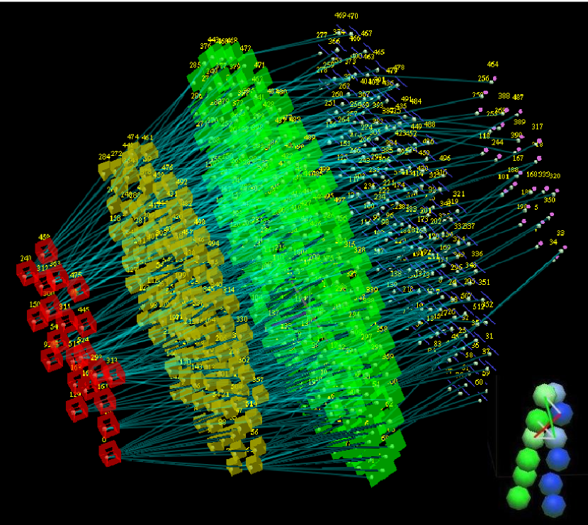
(a) stratification of assembly

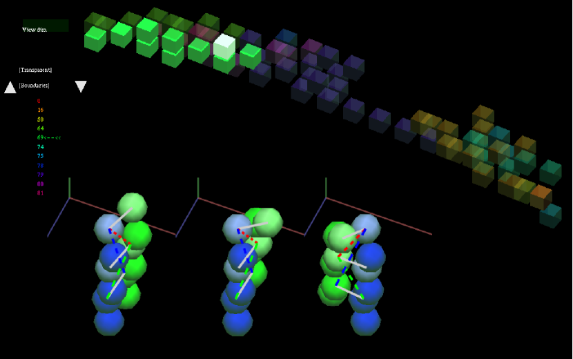
(b) top: Cayley points, bottom: Cartesian realizations

Figure 1: (a) Stratification: of assembly constraint system with parameters $n=$ 4 (red), 3 (yellow), 2 (green), 1 (white), 0 (purple). Strata of each dimension $j$ for the assembly constraint system visualized in the lower right inset are shown as nodes of one color and shape in a directed acyclic graph. Each node represents an active constraint region. Edges indicate containment in a parent region one dimension higher. (b) top: Realizable Cayley points (distance values) corresponding to one node in (a). Note a different use of color in the display of sample boxes in Cayley configuration space than in the stratification diagram. One Cayley point in the green group is highlighted. bottom: Three Cartesian realizations of the highlighted Cayley point. Each edge on a realization represents an active constraint graph and its chosen parameters.

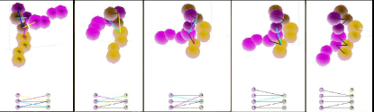
Figure 2: Adding constraints, removing parameters until $j=0$. top: Cartesian realizations with non-white segments: parameters and white segements constraints and bottom: activeConstraintGraph G yielding configurations with ever fewer free parameters as constraints are added one by one.

We represent the active constraint system for a region, by an active constraint graph (sometimes called contact graph) whose vertices represent the participating atoms (at least $3$ in each rigid component) and edges representing the active constraints between them. Between a pair of rigid components, there are only a small number of possible active constraint graph isomorphism types since there are at most $12$ contact vertices. For the case of $k=2$ these are listed in Figure 3, and for higher $k$ a partial list appears in Figure 4.

There could be regions of the stratification of dimension $j$ whose number of active constraints exceeds $6(k-1)-j$, i.e. the active constraint system is overconstrained, or whose active constraints are not all independent. Dependent constraints diminish the set of realizations. For entropy calculations, these regions should be tracked explicitly, but in the present paper, we do not consider these overconstrained regions in the stratification. Our regions are obtained by choosing any $6(k-1)-j$ independent active constraints.

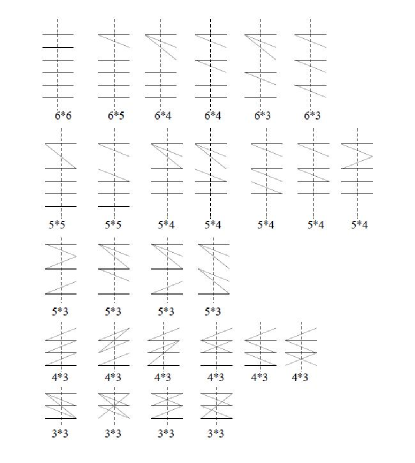
Figure 3: All active constraint graphs

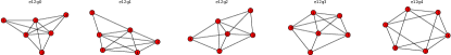
Figure 4: All non-isomorphic active constraint graphs with 6 vertices and 12 edges.

II.1.3 Convex representation of active constraint region and atlas

A new theory of Convex Cayley Configuration Spaces (CCCS) recently developed by the author SiGa:2010 gives a clean characterization of active constraint graphs whose configuration spaces are convex when represented by a specific choice of so-called Cayley parameters i.e., distance parameters between pairs of atoms (vertices in the active constraint graph) that are inactive in the given active constraint region (non-edges in the active constraint graph). See Figure 6. Such active constraint regions are said to be convexifiable, and the corresponding Cayley parameters are said to be its convexifying parameters. See Figures 5(a) 7

In general, the active constraint regions $R^{\prime}_{G}$ for an active constraint graph $G$, can be entirely convexified after ignoring the remainder of the assembly constraint system, namely the atom markers not in $G$ and their constraints. Fig. 6(a) The true active constraint region $R_{G}$ is subset of $R^{\prime}_{G}$, however the cut out regions are also defined by active constraints, hence they, too, could be convexified. See Figures 5(a), 7.

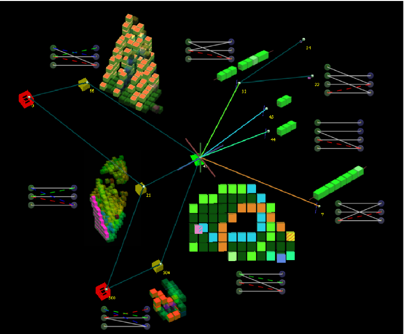
(a) Cayley charts of dimensions 1,2,3 attached to nodes.

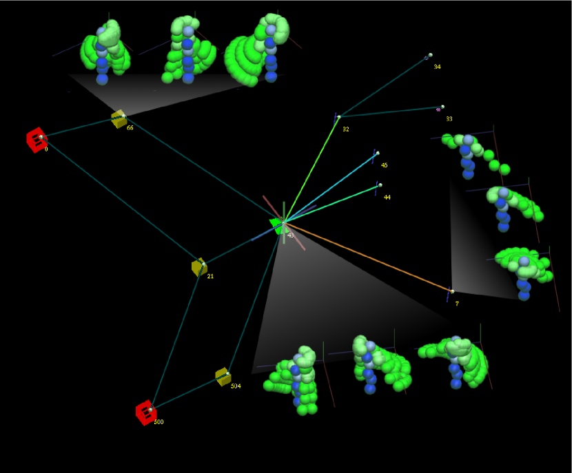
(b) Cartesian realizations of dimensions 1,2,3 attached to nodes.

Figure 5: Nested chains for one region of the atlas, i.e. nodes and paths in the directed acyclic graph of the stratification containing a 2d contraint region. center, green: a $2$d active constraint region. left, red and yellow: 4d and 3d parent regions containing the 2d region. right: 1d and 0d child regions. The G and chart are displayed next to each region. (a) The $2$-dimensional (exact, convex) chart in the center has a hole due to infeasible configurations also defined by Cayley parameter ranges, hence convex. Also, due to choice of different Cayley parameters, the same 2-dimensional region appears, without hole, in the $3$-dimensional parent charts as orange boxes top left, pink boxes middle left and red-orange boxes lower left; green boxes on right: 1-dimensional subregions. (b) Three grey fans attach the Cartesian realizations to their nodes as separate sweeps for different chirality of a region (the blue molecular unit is fixed without loss of generality).

When a constraint (edge $e$) not in $G$ becomes active (at a configuration $c$ in $R^{\prime}_{G}$), $G\cup\{e\}$ defines a child active constraint region $R_{G\cup e}$ containing $c$. This new region belongs to the stratum of the assembly configuration space that is of one lower dimension (Definition II.1.2) and defines within $R^{\prime}_{G}$ a boundary of the smaller, true active constraint region $R_{G}$. We can still choose the chart of $R^{\prime}_{G}$ as tight convex chart for $R_{G}$, but now region $R_{G\cup e}$ has an exact or tight convex chart of its own. Then the configurations in the region $R_{G\cup e}$ have lower potential energy since the configurations in that region lie in one more Lennard-Jones well. Hence they should be carefully sampled in free energy and entropy computations although the region has one lower effective dimension (e.g, represents a much narrower boundary channel). However, sampling in the larger parent chart of $R(G)$ (of one higher effective dimension) often does not provide adequate coverage of the narrow boundary region $R_{G\cup e}$. For example, Fig. 6(d) shows that providing a separate chart for each active constraint region can reveal additional realizations at the same level of sampling.

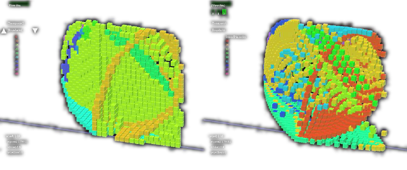
(a)

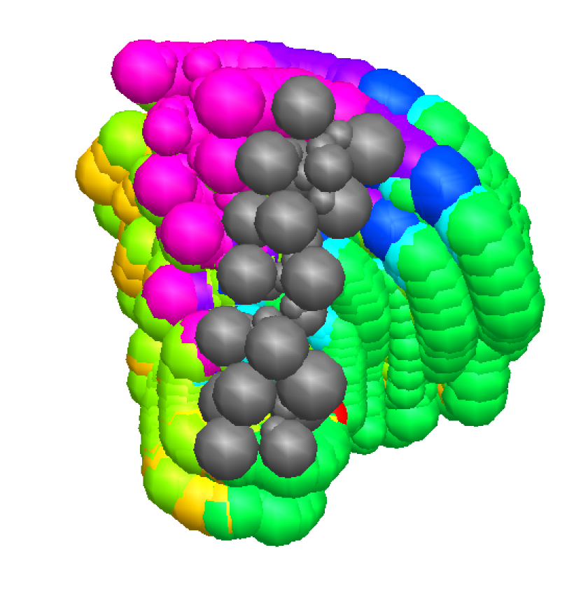
(b)

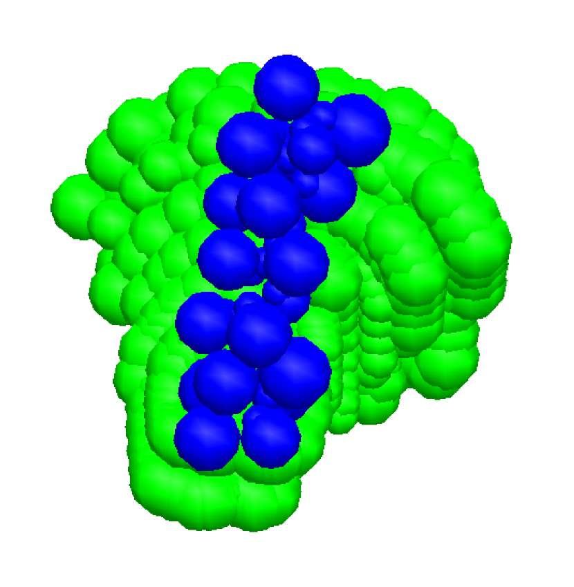
(c)

(d)

Figure 6: Top Left: atlas region showing interiors and boundaries sampled in its convexifying Cayley parameters; boundary/child regions sampled in their own Cayley parameters and mapped back to the parent region’s Cayley parameters (note increase in samples). Top Right: boundary/child regions sampled in their own Cayley parameters shown as sweeps around grey reference (toy) helix. Bottom Left: union of boundary regions sampled in parent’s Cayley parameters, shown as sweep around blue reference helix (notice (b) is bigger) Bottom Right: sweep of one of the boundary regions sampled in parent’s Cayley parameters is shown in red around gray reference helix; the sampling misses the other colored configurations in the same boundary region, obtained by sampling in its own Cayley parameters.

The Atlas of an assembly configuration space is a stratification of the configuration space into convexifiable regions. In Ozkan2011 , we have shown that molecular assembly configuration spaces with 2 rigid molecular components have an atlas. The software EASAL (Efficient Atlasing and Search of Assembly Landscapes) efficiently finds the stratification, incorporates provably efficient algorithms to choose the Cayley parameters SiGa:2010 that convexify an active constraint region, efficiently computes bounds for the parametrized convex regions ugandhar , and converts the parametrized configurations into standard cartesian configurations eigr2004 .

II.2 Preliminary Method: Cayley Sampling for Cartesian Uniformity

We discuss a preliminary method that highlights the issues and challenges that need to be addressed.

The Cayley points of the atlas need to be converted to Cartesian realizations as in Figure 7. An assembly configuration is a point in 6 dimensional Cartesian space representing the rotations and translations of one rigid molecular unit with respect to the fixed rigid molecular unit: ($x$, $y$, $z$, $\phi$, $\cos(\theta)$, $\psi$). For the active constraint graphs that occur in assembly Ozkan2011 ; Ozkan2014MainEasal , the Cartesian or Euclidean realization can be found using a sequence of tetrahedra constructions.

Observation 1

Every Cayley point in the exact convex chart $\Phi_{H}(G,F,d_{F},d_{H})$ has at least 1 and generically at most finitely many Cartesian realizations in the region $R_{G_{F}}$. See Figure 1(b).

Multiple Cartesian orientations correspond to same Cayley configuration. Those orientations are called flips of the Cayley configuration. The methods to be discussed below executed Cartesian sampling on each flip seperately. The flips can meet and bifurcate. For accurate configurational entropy computations, sampling in Cartesian space should maintain a measure of uniformity. The Cartesian sampling we aim for would be uniform on each flip. Ensuring uniformity when the flips are combined is beyond the scope of this paper. See fig. 7.

(a) $2$-d Cayley Space

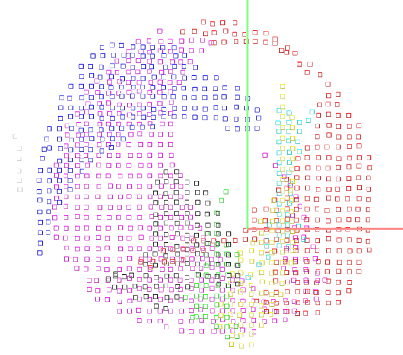
(b) Cartesian x, y view

Figure 7: Easal screenshot: a) $2$-D Jacobian sampling projected on Cayley space. b) $2$-D Jacobian sampling projected on $2$ independent Cartesian dimensions. c) $2$-D Jacobian sampling projected on $2$ independent Cartesian dimensions plus $1$ dependent dimension. All flips are colored differently.

However, while ensuring uniform Cartesian sampling on each flip, we would like to retain the advantages of Cayley sampling, including convexification of the active constraint regions. To obtain a measure of uniform sampling on Cartesian space while Cayley sampling, Cayley steps using the (inverse) Jacobian of the map from Cartesian to Cayley.

Definition II.1 (J)

The numerical Jacobian matrix $J$ defines a linear map F: Cayley space $\rightarrow$ Cartesian space, which is the best linear approximation of the function F near the configuration $p$. Each column of $J$ represents Cartesian changes after walking one step around $p$ = $(p_{1},p_{2},p_{3},p_{4},p_{5},p_{6})$ on Cayley space where $p_{i}$ is $i$th Cayley parameter. See Table 1. i.e. the first row of J is the changes along Cartesian $x$ dimension for each Cayley step.

	$p_{1}$	$p_{2}$	$p_{3}$	$p_{4}$	$p_{5}$	$p_{6}$
$x$	$\frac{\Delta x}{\Delta p_{1}}$	$\frac{\Delta x}{\Delta p_{2}}$	$\frac{\Delta x}{\Delta p_{3}}$	$\frac{\Delta x}{\Delta p_{4}}$	$\frac{\Delta x}{\Delta p_{5}}$	$\frac{\Delta x}{\Delta p_{6}}$
$y$	$\frac{\Delta y}{\Delta p_{1}}$	$\frac{\Delta y}{\Delta p_{2}}$	$\frac{\Delta y}{\Delta p_{3}}$	$\frac{\Delta y}{\Delta p_{4}}$	$\frac{\Delta y}{\Delta p_{5}}$	$\frac{\Delta y}{\Delta p_{6}}$
$z$	$\frac{\Delta z}{\Delta p_{1}}$	.	.	.	.	.
$\phi$	$\frac{\Delta\phi}{\Delta p_{1}}$	.	.	.	.	.
$\cos(\theta)$	$\frac{\Delta\cos(\theta)}{\Delta p_{1}}$	.	.	.	.	.
$\psi$	$\frac{\Delta\psi}{\Delta p_{1}}$	.	.	.	.	.

Table 1: Jacobian Matrix J

It is clear that the numerical Jacobian can be computed at each Cayley point, column-wise by finite differences.

In other words, let $s_{x}$, $s_{y}$, $s_{z}$, $s_{\phi}$, $s_{\cos(\theta)}$, $s_{\psi}$ be the sizes of the one step for each dimension on Cartesian space. Let $\Delta x$, $\Delta y$, $\Delta z$, $\Delta\phi$, $\Delta\cos(\theta)$, $\Delta\psi$ be the discretized Cartesian differences after one Cayley step. Then let $k_{1}=\Delta x/s_{x}$, $k_{2}=\Delta y/s_{y}$, $k_{3}=\Delta z/s_{z}$, $k_{4}=\Delta\phi/s_{\phi}$, $k_{5}=\Delta\cos(\theta)/s_{\cos(\theta)}$, $k_{6}=\Delta shi/s_{shi}$ be the coordinates of the Cartesian.
As criterion of uniformity, we could require the Euclidean 2-norm step distance $\|k_{1},k_{2},k_{3},k_{4},k_{5},k_{6}\|$ to be 1.

In order to achieve the above, we can try interpolation and binary search over the Cayley step size. This works reasonably well if the active constraint region being sampled is effectively 1-dimensional. However, for higher dimensions, since sampling is usually done one Cayley parameter at a time, although the Cartesian spacing may be maintained for samples along each Cayley line, the Cartesian trajectories corresponding to two Cayley lines may diverge.

In other words, the sampling adjustment should not be restricted only to $d$ sampling directions, where $d$ is the effective dimension of active constraint region being sampled. The entire volume of the $d$-dimensional neighborhood must be considered see fig. 8, and Jacobian adjustments are required to address both the step size and direction issues.

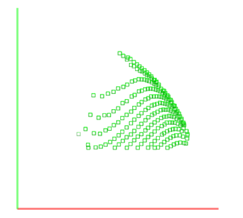
(a) Uniform Cartesian sampling projected on Cayley Space

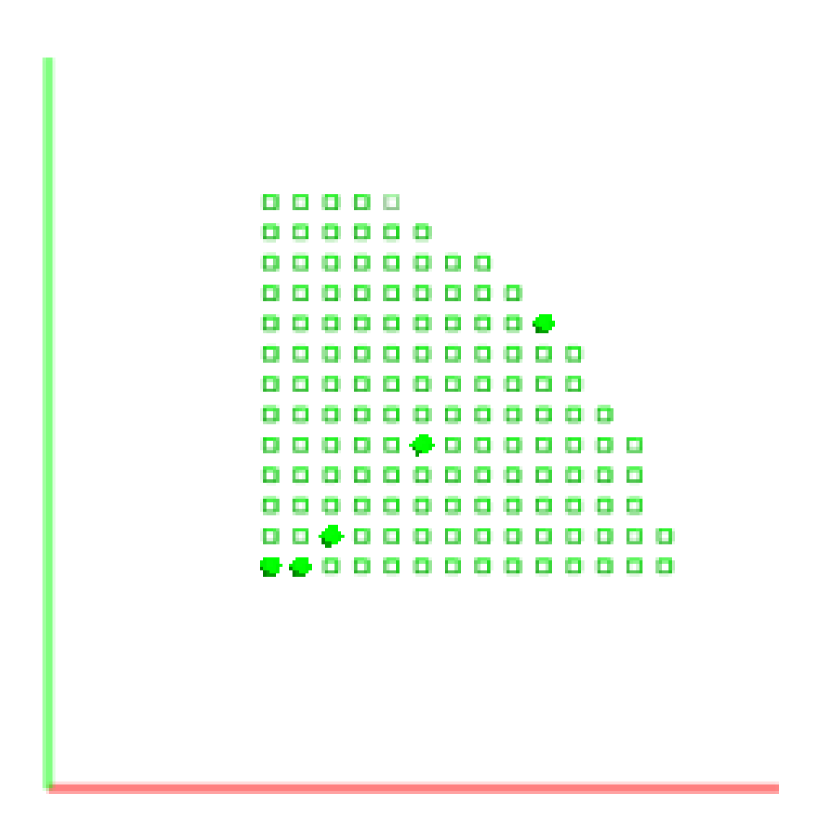
(b) Uniform Cayley sampling projected on Cayley Space

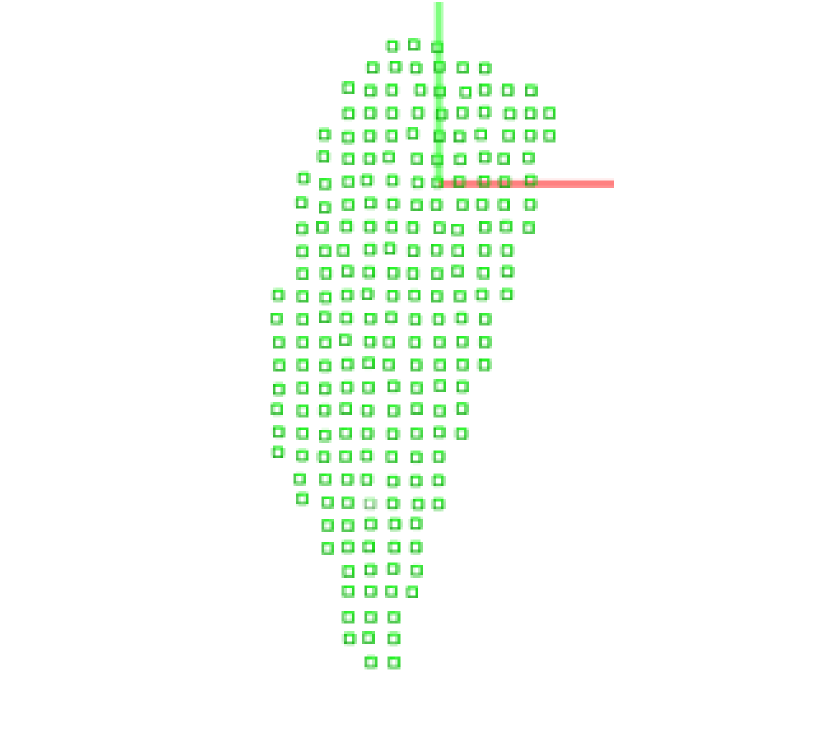
(c) Uniform Cartesian sampling projected on Cartesian Space

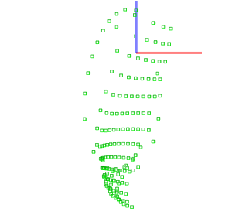
(d) Uniform Cayley sampling projected on Cartesian Space

Figure 8: Easal screenshot: Different sampling methods projected on both $2$d Cayley space and Cartesian space. Notice the need of walking directionally (not just horizontal and vertical) on Cayley space in order to have uniform sampling on Cartesian space.

Definition II.2

The Orthogonal Cartesian Step Matrix $C$
Let $C$ be the matrix where each column represents expected Cartesian changes after one directional Cayley step. See Table 2. We would like to walk orthogonally in Cartesian space.

$s_{x}$	0	0	0	0	0
0	$s_{y}$	0	0	0	0
0	0	$s_{z}$	0	0	0
0	0	0	$s_{\phi}$	0	0
0	0	0	0	$s_{\cos(\theta)}$	0
0	0	0	0	0	$s_{\psi}$

Table 2: Cartesian Step Matrix $C$: diagonal matrix with Cartesian steps as diagonal entries.

Definition II.3

The Cayley Step Matrix $S$ corresponding to $C$
Let $S$ be the matrix of Cayley steps such that when adjusted by the Jacobian results in $C$. i.e. $JS=C$. $S$ is the numerical $J_{inv}C$. See Table 3.
Each column of $S$ represents one directional Cayley step that is predicted to yield orthogonal stepping in Cartesian space.

	$\overrightarrow{s_{1}}$	$\overrightarrow{s_{2}}$	$\overrightarrow{s_{3}}$	$\overrightarrow{s_{4}}$	$\overrightarrow{s_{5}}$	$\overrightarrow{s_{6}}$
$p_{1}$	$s_{11}$	$s_{21}$	.	.	.	.
$p_{2}$	$s_{12}$	$s_{22}$	.	.	.	.
$p_{3}$	$s_{13}$	$s_{23}$	.	.	.	.
$p_{4}$	$s_{14}$	$s_{24}$	.	.	.	.
$p_{5}$	$s_{15}$	$s_{25}$	.	.	.	.
$p_{6}$	$s_{16}$	$s_{26}$	.	.	.	.

Table 3: Directional Cayley Steps

II.2.1 Issues

Ill-conditioned Jacobian:
Jacobian matrix is by definition an linear approximation of the nonlinear map $F:\textit{Cayley space}\rightarrow\textit{Cartesian space}$. The Jacobian can be ill-conditioned and sensitive to small changes and numerical errors in its arguments.

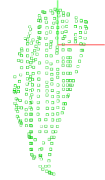
Figure 9: Easal screenshot: Jacobian sampling projected on Cartesian Space fails to satisfy uniformity for some regions.

What Cayley trajectory to follow to ensure comprehensive coverage?
In uniform Cayley sampling, the Cayley parameters are walked one by one (grid sampling on Cayley space). With the above Jacobian adjustments to Cayley step direction, such grid sampling is impossible. Hence it is important to have a systematic method to determine what path to follow avoiding repetitions and ensuring coverage. For a single Cartesian dimension the corresponding Cayley direction is specified by the Jacobian adjustment in every step. As in the previous approach (without direction adjustment) it is not clear how to generalize this to higher dimensional regions. While uniform Cayley sampling comprehensively covers Cayley space and thereby also Cartesian space. This property is not generally preserved by the use of Jacobian adjustments to stepping direction.

II.3 Recursive, Adaptive Cayley Sampling

We propose an Iterative Jacobian computation method with adapted step magnitude and direction, followed by a recursive Cayley trajectory determination method to deal with the issues discussed in the previous subsection. We will use $S,C,J$ to denote the $d\times d$ matrices of Cayley steps, Cartesian steps, Jacobian, respectively, as described above, where $d$ is dimension of the active constraint region that is currently being sampled. Recall that the value $d$ is at most 6 for packing of $2$ rigid molecules. The first two subsections deal separately with the two issues mentioned above: Illconditioning of the Jacobian and Cayley sampling trajectory.

II.3.1 Ill-conditioning: Iterative Jacobian computation

The Jacobian matrix would give the best approximation, if the Cayley steps that are used to create Jacobian matrix are close to the output Cayley steps as a result of Jacobian adjustment. In order to achieve best approximation, we iterate on Cayley directions and magnitudes until convergence. See Algorithm 1.

computeCayleyDirectionIteratively

input : $S,C$, config

output : $S$ // final Cayley steps

$J$ := computeJacobian($S$, config)

$K:=J_{inv}C$; // $K$ is Cayley transformer(definition below)

$S:=SK$;

if $K$ is not close to identity matrix then

       return computeCayleyDirectionIteratively($S,C$, config);

else

      return $S$;

end if

Algorithm 1 computeCayleyDirectionIteratively

Note that when the the numerical Jacobian is computed, the $i$th column of $J$ represents Cartesian changes after walking one step on Cayley parameter $p_{i}$. The $i$th column of $J$ is divided to $\Delta p_{i}$ which is a scalar value. See Table 1. However, now the $i$th column of $J$ represents Cartesian changes after walking one directional Cayley step $\overrightarrow{s_{i}}$ that is $i$th column of $S.$ Hence $\Delta\overrightarrow{s_{i}}$ is a vector having components in all Cayley parameters $p_{i}$. So we redefine the Jacobian matrix as:

	$\overrightarrow{s_{1}}$	$\overrightarrow{s_{2}}$	$\overrightarrow{s_{3}}$	$\overrightarrow{s_{4}}$	$\overrightarrow{s_{5}}$	$\overrightarrow{s_{6}}$
$x$	$\Delta x_{s_{1}}$	$\Delta x_{s_{2}}$	$\Delta x_{s_{3}}$	$\Delta x_{s_{4}}$	$\Delta x_{s_{5}}$	$\Delta x_{s_{6}}$
$y$	$\Delta y_{s_{1}}$	$\Delta y_{s_{2}}$	$\Delta y_{s_{3}}$	$\Delta y_{s_{4}}$	$\Delta y_{s_{5}}$	$\Delta y_{s_{6}}$
$z$	$\Delta z_{s_{1}}$	.	.	.	.	.
$\phi$	$\Delta\phi_{s_{1}}$	.	.	.	.	.
$\cos(\theta)$	$\Delta\cos(\theta)_{s_{1}}$	.	.	.	.	.
$\psi$	$\Delta\psi_{s_{1}}$	.	.	.	.	.

Table 4: Redefined Jacobian Matrix J

With the redefined Jacobian $J$ $J_{inv}C$ has a new interpretation.

Definition II.4 (The Cayley transformer matrix $K$)

Let $K$ be the Cayley transformer matrix such that when adjusted by the Jacobian we obtain $C$. i.e. $JK=C$
See Table 5.
Each column of $K$ contains the coefficients of current Cayley steps that will lead to new direction in Cayley space that will yield orthogonal sampling in Cartesian space. See fig. 10.

$k_{1}\_s_{1}$	$k_{2}\_s_{1}$	.	.	.	.
$k_{1}\_s_{2}$	$k_{2}\_s_{2}$	.	.	.	.
$k_{1}\_s_{3}$	$k_{2}\_s_{3}$	.	.	.	.
$k_{1}\_s_{4}$	$k_{2}\_s_{4}$	.	.	.	.
$k_{1}\_s_{5}$	$k_{2}\_s_{5}$	.	.	.	.
$k_{1}\_s_{6}$	$k_{2}\_s_{6}$	.	.	.	.

Table 5: Cayley Transformer $K$

In order to compute $K$, $J_{inv}$ needs to be computed, hence $J$ has to be a square matrix. At first glance, computing the inverse of Jacobian matrix can be worrying since the Jacobian matrix is $6\times d$ matrix now. However, if Cayley space is $d$ dimensional ($d<6$), then in fact the Cartesian basis has only $d$ independent vectors Hence, we can crop $6-d$ rows of Jacobian matrix to make it $d\times d$ square matrix. Here the question is then how to best find those dependent $6-d$ rows. Among all ${6\choose d}$ combinations of $d\times d$ submatrix of $J$, pick the one that gives best determinant.

Figure 10 illustrates the transformation of from initial orthogonal Cayley basis to the new directed Cayley basis. At each iteration, new Cayley transformer matrix $K$ is computed.

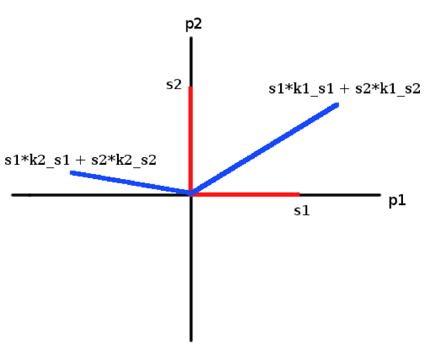
(a) $2$D Cayley basis transformation

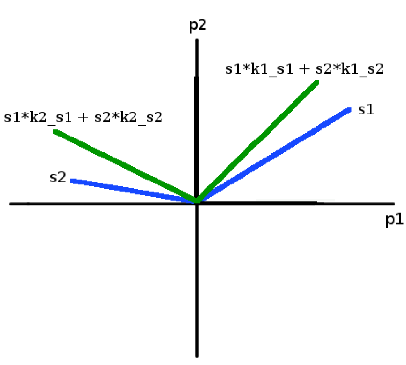
(b) $2$D Cayley basis transformation second iteration

Figure 10: Initial Cayley steps are orthogonal to Cayley parameter space ($p_{1}$, $p_{2}$). $K$ is first applied to inital Cayley steps(red lines) to achieve new Cayley basis(blue lines). Then applied to current Cayley basis (blue lines) to achieve new Cayley basis (green lines).

The following method can be used to speed up convergence of the above method or for finer adjustments - its convergence, however, is not guaranteed. It works best for a small number of dimensions.

II.3.2 Illconditioning: Adaptive magnitude and direction:

In order to correct the direction distortions, the idea is to precompute, for the $i$th direction Cartesian step, how much distortion is caused in the $j$th direction. Adjust the $j$th direction by using $j$th Cayley step that is dedicated to the $j$th Cartesian dimension and subtract those distortion adjustments step. See Algorithm 2.

adaptiveMagnitudeAndDirection

input : $S$, $C$, config, $i$, threshold // $i$:direction

output :  out_config

new_config := adaptiveMagnitude($S(i),C(i,i)$, config, $i$, threshold);

if  new_config is still failed due to inaccuracy of Jacobian then

       return failed

end if

$\gamma$ := the distortions on all Cartesian directions between new_config and expected new_config

$\gamma_{c}$ := $\gamma$ corresponding to the deviation in terms Cartesian unit steps.

for  each $j$th Cartesian direction  do

       set Cayley step $s_{j}$ to -$S(j)\gamma_{c}(j)$ to reset the deviation on $j$th direction of Cartesian space.

       temp_config := adaptiveMagnitude($s_{j}$, $\gamma(j)$, new_config, $j$, threshold);

       if  able to fix distortion  then

             update new_config to be temp_config consecutively

       end if

      

end for

// final check if distorted or not after cumulative distortion fixes

compute the change on Cartesian direction $i$ between $config$ and new_config

ratio := the change / expected Cartesian step $C(i,i)$

if  ratio is within [1 $\pm$ threshold]  then

       return new config;

else

       return failed;

end if

Algorithm 2 adaptiveMagnitudeAndDirection

The method Algorithm 3 called above has adaptive step size to compensate for the inaccuracy of the Jacobian. It uses binary search on the step size (multiplier to the column) until it gets the desired step size. The adaptive search stops if stepping ratio is within [1 $\pm$ threshold].

adaptiveMagnitude

input : $s_{i}$, $c_{i}$, $config$, $i$, $threshold$, $min\_s_{i}$, $max\_s_{i}$ // $s_{i}$: $i$th Cayley step, $c_{i}$: $i$th Cartesian step, $i$:direction

output :  out_config

update $min\_s_{i}$ and $max\_s_{i}$ by comparing $s_{i}$

if  $min\_s_{i}$ $>$ $max\_s_{i}$  then

       return failed;

end if

compute new_config by walking from $config$ by step := $s_{i}$

if  new_config is realizable  then

       compute the change on Cartesian dimension $i$ between $config$ and new_config

       ratio := the change / expected Cartesian step $c_{i}$

       if  ratio is within [1 $\pm$ threshold]  then

             return new config;

      else

             $s_{i}$ := $s_{i}$ / ratio;

             return adaptiveMagnitude($s_{i}$, $c_{i}$, $config$, $i$, $threshold$, $min\_s_{i}$, $max\_s_{i}$);

       end if

      

else

       $s_{i}$ := ($min\_s_{i}$ + $max\_s_{i}$)/2 ;

       return adaptiveMagnitude($s_{i}$, $c_{i}$, $config$, $i$, $threshold$, $min\_s_{i}$, $max\_s_{i}$);

end if

Algorithm 3 adaptiveMagnitude

As mentioned earlier, these patch ups work well in practice for fine tuning or for small number of dimensions. Convergence is not guaranteed in theory. For the high dimensions, the adjustment of one dimension may increse distortion in another.
Hence, correctness of input Cayley direction matrix $S$ is crucial, for which the Cayley trajectory becomes important, in order to achieve the best approximation of $S$ by recursive Jacobian computation in Algorithm 1 above.
We discuss the issue of Cayley trajectory next.

II.3.3 Recursive Cayley trajectory

Recursive Cayley sampling walks in every direction of Cartesian space at every step. If it hits a boundary, then it does not proceed forward at that point. Since in our assembly settings, feasible regions in Cartesian space are connected RecursiveSampling will find a path to cover the region.
This way, in the case of a nested infeasible region inside a feasible region such as a steric boundary, just the boundary of the infeasible region is sampled (the inside of the steric region is not inefficiently sampled and discarded).

In order to keep track if specific points in Cartesian grid have been visited, a boolean map $M$ is used as Cartesian grid coordinate system of appropriate size. See Algorithm 4.

RecursiveSampling

input : $S$, $C$, $M$, cartpoint, config, threshold // $M$:the matrix keeps track of a point is visited or not, cartpoint: the vector for current Cartesian point in $M$

output : $R$ // set of configs

$R$ := $R$ + config;

$new\_S$ := computeCayleyDirectionRecursively($S$, $C$, config); // uses S from previous point to converge faster.

for each Cartesian dimension $i$ and reverse direction of $i$ do

       new_cartpoint:= cartpoint;

       new_cartpoint($i$) := $\pm$1; // -1 if reverse direction

       if  $M$(new_cartpoint) is not visited before  then

             new_config := adaptiveMagnitudeAndDirection($new\_S$, $C$, config, $i$, threshold);

             if  new_config is failed // due to Cartesian boundary or Jacobian was not good enough approximate to walk one step within the threshold then

                   new_config := jumpToDisconnectedRegion($S(i)$, $M$, cartpoint, config ); // uses $S(i)$ that is previous Cayley step

                   update new_cartpoint of new_config;

             end if

            if  new_config is succesfully computed then

                   set M(new_cartpoint) to true to be visited

                   if  new_config doesnot hit any boundary like sterics or etc. then

                         RecursiveSampling($new\_S$, $C$, $M$, new_cartpoint, new_config, threshold);

                        

                   end if

                  

             end if

            

       end if

      

end for

Algorithm 4 RecursiveSampling

Note: Consecutive small deviations that are within a tolerance at each step may result in change of the direction of the path. In order to correct this:
Usually, expected step size is set to be $C(i,i)$ for $i$th Cartesian direction in Algorithm 2. However if previous point is deviated for the amount of $\mu$ from the original path along an arbitrary Cartesian direction, then the next step size should be set to $C(i,i)-\mu$.

Narrow Cartesian Gates As pointed out earlier, connected Cartesian regions permit comprehensive sampling, in principle. However, since the sampling is discrete, and Jacobian can be illconditioned, the issue of narrow gates at unknown locations in Cartesian regions needs to be dealt with. Here we leverage the fact that Cayley space is convex. The idea is to use previous Cayley step that stayed in feasible Cartesian region as a new step. We can guarantee that this will not reverse direction or repeat sample in Cartesian space. In short, for every point close to the boundary in Cartesian, we check if it is possible to walk on Cayley space.

jumpToDisconnectedRegion

input : $s_{i}$, $M$, cartpoint, config // $M$:the matrix keeps track of a Cartesian point is visited or not, cartpoint: the vector for current Cartesian point in $M$

output : new_config

compute new_config by walking from $config$ by step := $s_{i}$ // this is a jump on Cartesian space

if  new_config stays in Cayley boundary then

       compute new_cartpoint of new_config;

       if  $M$( new_cartpoint ) is not visited before  then

             if  new_cartpoint moves at least $1$ Cartesian step from cartpoint then

                   return new_config;

             end if

            

       end if

      

end if

return failed;

Algorithm 5 jumpToDisconnectedRegion

III Results

Recall that our goal is to combine the advantages of Cayley sampling with that of uniform sampling in Cartesian. The former permits topological roadmapping, as well as guaranteed isolation and coverage of effectively low dimensional, low potential energy regions relatively much more efficiently and with much fewer samples compared to MonteCarlo or simply Cartesian grid sampling, with the additional efficiency of not leaving the feasible regions, and not discarding samples. Ozkan2011 ; Ozkan2014MainEasal .

Since the methods of this paper have preserved the above advantages, the emphasis of our comparison here is only the uniformity of sampling in Cartesian. For this purpose only, we compare the original EASAL Ozkan2011 ; Ozkan2014MainEasal , modified EASAL-jacobian (this paper) and uniform Cartesian grid sampling of assembly configuration spaces of $2$ rigid molecules with about $20$ atoms. We used last 20 residues of HiaPP(human islet amyloid polypeptide PDB-2KJ7) which contain the 6 residues where it differs from RiaPP (rat islet amyloid polypeptide PDB-2KB8). See fig. 11. We created the 5D stratum (regions with a single active constraint) of both versions of EASAL atlas for $2$ assembling HiaPP molecules and separately, for $2$ assembling RiaPP molecules. For comparison purposes, in both cases, a reference Grid is generated, which is designed to cover the part of the configurational space of interest, i.e., observed in nature.

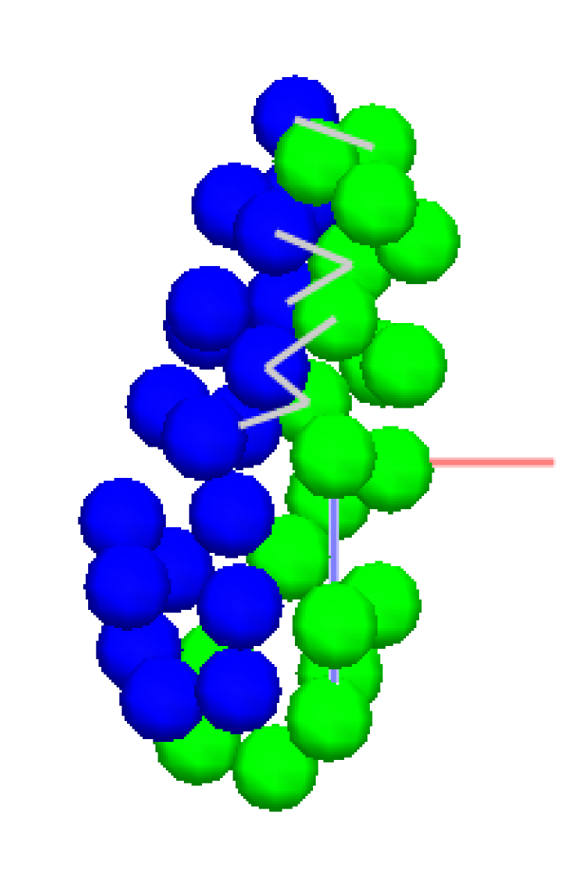
(a) HiaPP

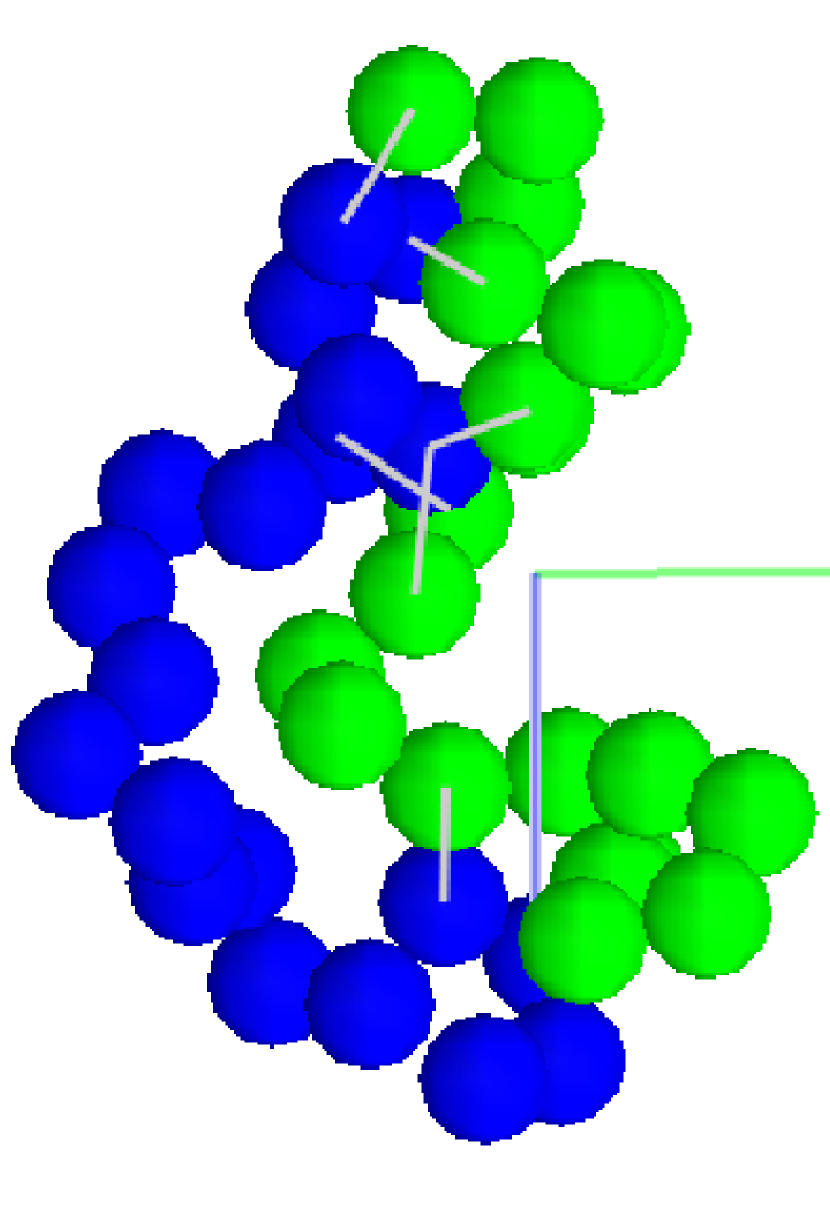
(b) RiaPP

Figure 11: Easal screenshot: displays the molecule

III.1 Multigrid

Both versions of EASAL are designed to isolate and sample each active constraint region. In addition, EASAL-Jacobian samples each such region uniformly in Cartesian. Yet, when we combine all such regions, those regions where more pairs of atoms are in their Lennard-Jones wells (regions with more active constraints) will have denser sampling. i.e. EASAL tends to oversample the lower energy regions. This is a positive feature of EASAL that we preserve in EASAL-Jacobian. Since the 5D strata of the atlas generated by both versions of EASAL would sample a configuration that has $l$ active constraints $l$ times (once for each of the 5D active constraint regions in which the configuration lies), the meaningful comparison would require similarly replicating such configurations in the grid, which we call the multigrid.

III.2 Grid Generation

• The Grid is uniform along the Cartesian configuration space.

• The bounds of the Cartesian configuration space for both Grid and EASAL are:
  $X,Y:$ -26 to 26 Angstroms
  $Z:$ -7 to 7 Angstroms
  

• The angle parameters are described in Euler angles representation (Cardan angle ZXZ).
  $\phi,\psi:-\pi$ to $\pi$

• Inter principal-axis angle $\theta<30.0$ degrees where $\theta=a\cos(uv)$ where $u$ and $v$ are the principal axis of each rigid body. I.e. $u$ and $v$ are eigenvectors of the inertia matrix.

• Additionally, there is the pairwise distance lower bound criterion:
  For all atom pairs $i,j$ belonging to different rigid molecular components, $d_{ij}>0.8∗(r_{i}+r_{j})$ where $i$ and $j$ are residues, $d_{ij}$ is the distance for residues $i$ and $j$, $r_{i}$ and $r_{j}$ are the radius of residue atoms $i$ and $j$.
  

• 147 Million grid configurations are generated in this manner.

• Over 93% of them are discarded to ensure at least one pair $d_{ij}<r_{1}+r_{2}+0.9$, i.e, an active constraint and to eliminate collisions. About $9.6$ Million grid configurations remain.

III.3 Computational Time/Resources for EASAL

The specification of the processor that EASAL executed is Intel Core 2 Quad CPU Q9450 @ 2.66GHz x 4 with Memory:3.9 GiB.
EASAL-Jacobian for input HIAPP took 2 days 9 hours 20 minutes(3440 minutes) and for input RIAPP took 3 days 14 hours 44 minutes(5204 minutes).
EASAL for input HIAPP took 5 hours 40 minutes(340 minutes) and for input RIAPP took 6 hours 52 minutes(412 minutes).

III.4 Epsilon Coverage

Ideally, we would expect each Grid point to be covered by at least one EASAL sample point that is situated in an $\epsilon$-cube centered around a Grid point with a range of $2\epsilon$ in each of the 6 dimensions.

• The value of $\epsilon$ is computed as follows: $\epsilon$ = ($\#$ of Grid points / # of Easal points)${}^{1/6}/2$

• We set $\epsilon$ to be $\lceil\epsilon\rceil$ since grid points are by definition a discrete number of steps from each other.

• In order to compute the coverage, we assign each EASAL sample to its closest Grid point. Call those Grid points EASAL-mapped Grid points. We say that a Grid point $p$ is covered if there is at least one EASAL-mapped Grid point within the $\epsilon$-cube centered around $p.$

• $\epsilon$ for HiaPP: The number of samples generated by Grid, EASAL and EASAL-jacobian were 9,619,435/194,595/2,861,926 respectively. The corresponding $\epsilon$ for EASAL is $\lceil 49.4331^{1/6}/2\rceil=\lceil 0.957869\rceil$ and for EASAL-Jacobian is $\lceil 3.36118^{1/6}/2\rceil=\lceil 0.611954\rceil$.

• $\epsilon$ for RiaPP: The number of samples generated by Grid, EASAL and EASAL-jacobian were 13,267,314/319,016/4,744,878 respectively. The corresponding $\epsilon$ for EASAL is $\lceil 41.5882^{1/6}/2\rceil=\lceil 0.930676\rceil$ and for EASAL-Jacobian is $\lceil 2.79613^{1/6}/2\rceil=\lceil 0.593467\rceil$.

III.5 Coverage Results

The results show that $96.21\%$ of Grid points are covered by EASAL-jacobian for HiaPP and $96.14\%$ of Grid points are covered for RiaPP.

For basic EASAL, $85.03\%$ of Grid points are covered for HiaPP and $85.46\%$ of Grid points are covered for RiaPP.

Hence EASAL-jacobian is verified to have almost full coverage.

III.6 Density Distribution

The fig. 12 shows the sampling distribution over Cartesian $x,y$ space for Grid, MultiGrid, EASAL-jacobian and EASAL. The reddish regions are considered to be the lower energy regions.

EASAL and EASAL-jacobian is run for the majority of active constraint regions. i.e. it generated most of the 5D strata of the atlas. Hence a configuration with $l$ active constraints is sampled close to $l$ times. Then we would expect density distribution for EASAL and EASAL-jacobian to lay in between Grid and MultiGrid.

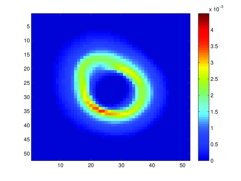
(a) HiaPP: GRID

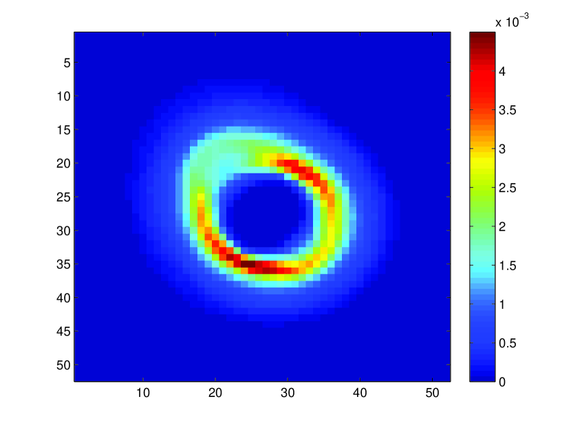
(b) HiaPP: MULTIGRID

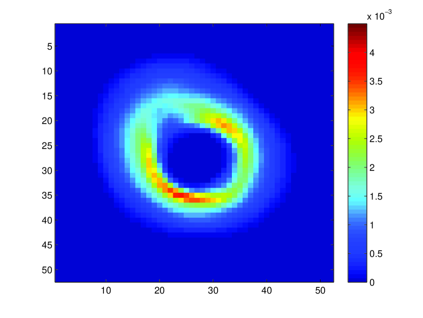
(c) HiaPP: EASAL jacobian sampling

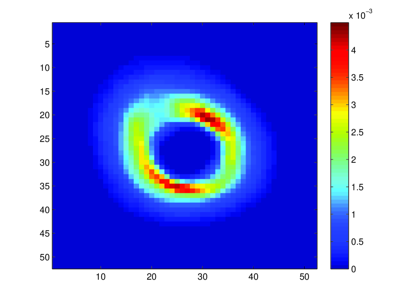
(d) HiaPP: EASAL sampling

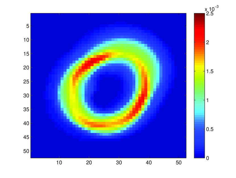
(e) RiaPP: GRID

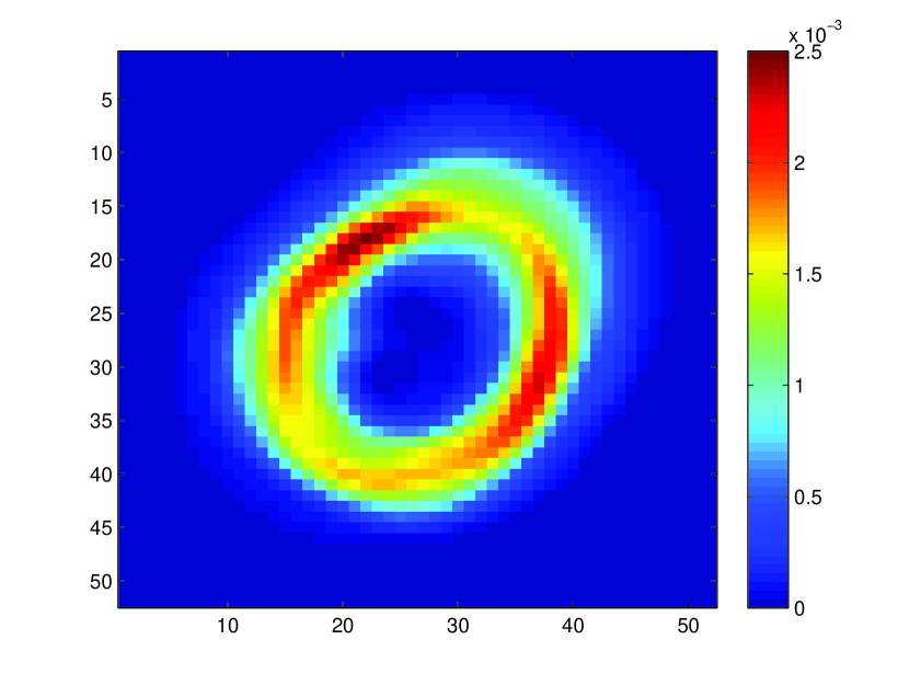
(f) RiaPP: MULTIGRID

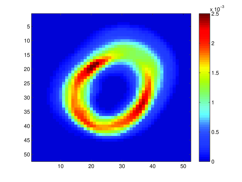
(g) RiaPP: EASAL jacobian sampling

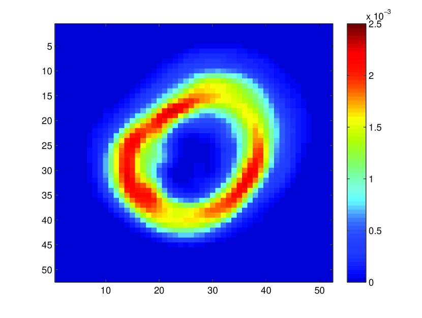
(h) RiaPP: EASAL sampling

Figure 12: horizontal axis: Cartesian $x$ coordinate, vertical axis: Cartesian Y coordinate
color code: the ratio of ”the # of points that lay in an $\epsilon$-cube centered around Grid point $x,y$” over ”total # of points”

IV Discussion

A key goal is to find hybrid methods that combine the complementary strengths of EASAL with prevailing methods. A useful development would be a gradual tuning parameter, or flexible choice to allow a smooth transition from uniform sampling on Cartesian space to uniform sampling on Cayley space. Such a tuning parameter would improve EASAL’s flexibility to go from the basic-EASAL to mimicking multigrid and MC, while still maintaining the advantages of EASAL. This would additionally make it easier to develop hybrids between EASAL and prevailing methods leveraging the complementary advantages. Extensive comparison of EASAL’s and MC’s performances have been reported in Ozkan2014MC .

Algorithm 5 can be used with some modifications as an independent component to improve ergodicity of regular MC sampling in order to help jump to a region separated by a narrow channel, or to pass a high energy barrier.

Some aspects of the recursive and adaptive jacobian computation and sampling method presented here require a seed matrix or direction or value starting from which they iterate. These include Algorithms 1, and 2. In most cases, a good choice of seed is crucial for rapid convergence.

V Conclusion

We have presented a modification to EASAL that combines the advantages of Cayley sampling with that of uniform sampling in Cartesian. The former permits topological roadmapping, as well as guaranteed isolation and coverage of effectively low dimensional, low potential energy regions relatively much more efficiently and with much fewer samples compared to MonteCarlo or simply Cartesian grid sampling, with the additional efficiency of not leaving the feasible regions, and not discarding samples.

The modification of EASAL presented here features careful and versatile use of the Jacobian of the maps between Cartesian and Cayley to provide iterative, recursive and adaptive methods to achieve uniform sampling in Cartesian while preserving the advantages of sampling in Cayley space. While the results are encouraging when we compare the basic EASAL and the modified EASAL on dimer assembly configuration spaces of HiaPP and RiaPP, there is much room for exploring and tapping the continuum of methods that traverse the distance between EASAL and other prevailing methods.

References

- [1] Ioan Andricioaei and Martin Karplus. On the calculation of entropy from covariance matrices of the atomic fluctuations. The Journal of Chemical Physics, 115(14):6289, 2001.
- [2] U. Chittamuru. Efficient Iterative algorithm for bounding and sampling the Cayley configuration space of partial 2-trees in 3D. M.S. Thesis University Of Florida, 2010.
- [3] Jonathan P.K. Doye and David J. Wales. The structure of (C60)N clusters. Chemical Physics Letters, 262(1-2):167–174, November 1996.
- [4] Domenico Gazzillo, Achille Giacometti, Riccardo Fantoni, and Peter Sollich. Multicomponent adhesive hard sphere models and short-ranged attractive interactions in colloidal or micellar solutions. Physical Review E, 74(5):051407, November 2006.
- [5] David Gfeller, David Morton De Lachapelle, Paolo De Los Rios, Guido Caldarelli, and Francesco Rao. Uncovering the topology of configuration space networks. Physical Review E - Statistical, Nonlinear and Soft Matter Physics, 76(2 Pt 2):026113, 2007.
- [6] M. H. J. Hagen, E. J. Meijer, G. C. A. M. Mooij, D. Frenkel, and H. N. W. Lekkerkerker. Does C60 have a liquid phase? Nature, 365(6445):425–426, September 1993.
- [7] Martha S Head, James A Given, and Michael K Gilson. Mining minima : Direct computation of conformational free energy. The Journal of Physical Chemistry A, 101(8):1609–1618, 1997.
- [8] Ulf Hensen, Oliver F Lange, and Helmut Grubm ller. Estimating absolute configurational entropies of macromolecules: The minimally coupled subspace approach. PLoS ONE, 5(2):8, 2010.
- [9] Vladimir Hnizdo, Eva Darian, Adam Fedorowicz, Eugene Demchuk, Shengqiao Li, and Harshinder Singh. Nearest-neighbor nonparametric method for estimating the configurational entropy of complex molecules. Journal of Computational Chemistry, 28(3):655–668, 2007.
- [10] Vladimir Hnizdo, Jun Tan, Benjamin J Killian, and Michael K Gilson. Efficient calculation of configurational entropy from molecular simulations by combining the mutual-information expansion and nearest-neighbor methods. Journal of Computational Chemistry, 29(10):1605–1614, 2008.
- [11] Miranda Holmes-Cerfon, Steven J Gortler, and Michael P Brenner. A geometrical approach to computing free-energy landscapes from short-ranged potentials. Proceedings of the National Academy of Sciences of the United States of America, 110(1):E5–14, January 2013.
- [12] Wonpil Im, Michael Feig, and Charles L Brooks. An implicit membrane generalized born theory for the study of structure, stability, and interactions of membrane proteins. Biophysical Journal, 85(5):2900–2918, 2003.
- [13] Léonard Jaillet and Josep Maria Porta. Path planning with loop closure constraints using an atlas-based RRT. In International Symposium on Robotics Research (ISRR), 2011.
- [14] M. Karplus and J.N. Kushick. Method for estimating the configurational entropy of macromolecules. Macromolecules, 14(2):325–332, 1981.
- [15] Benjamin J Killian, Joslyn Yundenfreund Kravitz, and Michael K Gilson. Extraction of configurational entropy from molecular simulations via an expansion approximation. The Journal of chemical physics, 127(2):024107, 2007.
- [16] Bracken M. King, Nathaniel W. Silver, and Bruce Tidor. Efficient calculation of molecular configurational entropies using an information theoretic approximation. The Journal of Physical Chemistry B, 0(ja):null, 0.
- [17] Zaizhi Lai, Jiguo Su, Weizu Chen, and Cunxin Wang. Uncovering the properties of energy-weighted conformation space networks with a hydrophobic-hydrophilic model. International Journal of Molecular Sciences, 10(4):1808–1823, 2009.
- [18] T Lazaridis and M Karplus. Effective energy function for proteins in solution. Proteins, 35(2):133–152, 1999.
- [19] Themis Lazaridis. Effective energy function for proteins in lipid membranes. Proteins, 52(2):176–192, 2003.
- [20] Shawn Martin, Aidan Thompson, Evangelos A Coutsias, and Jean-Paul Watson. Topology of cyclo-octane energy landscape. The Journal of chemical physics, 132(23):234115, June 2010.
- [21] Guangnan Meng, Natalie Arkus, Michael P. Brenner, and Vinothan N. Manoharan. The free-energy landscape of clusters of attractive hard spheres. Science (New York, N.Y.), 327(5965):560–3, January 2010.
- [22] Aysegu Ozkan and Meera Sitharam. Easal: Efficient atlasing, analysis and search of molecular assembly landscapes. In Proceedings of the ISCA 3rd International Conference on Bioinformatics and Computational Biology, BICoB-2011, 2011.
- [23] Aysegul Ozkan, JC Flores-Canales, and Meera Sitharam. Geometrical algorithm for enhanced sampling of compact configurations in protein docking problem. (on arxiv), 2014.
- [24] Aysegul Ozkan, James Pence, Ruijin Wu, Troy Baker, Joel Willoughbyand, Jorg Peters, and Meera Sitharam. Easal: Software architecture and functionalities. (on arxiv), 2014.
- [25] Aysegul Ozkan, Ruijin Wu, Jorg Peters, and Meera Sitharam. Efficient atlasing and sampling of assembly free energy landscapes using easal: Stratification and convexification via customized cayley parametrization. (on arxiv), 2014.
- [26] Jörg Peters, JianHua Fan, Meera Sitharam, and Yong Zhou. Elimination in generically rigid 3d geometric constraint systems. In Proceedings of Algebraic Geometry and Geometric Modeling, pages 27–29, Nice, September 2004. Springer Verlag,1-16,2005.
- [27] Josep M Porta, Lluís Ros, Federico Thomas, Francesc Corcho, Josep Cantó, and Juan Jesús Pérez. Complete maps of molecular-loop conformational spaces. Journal of computational chemistry, 28(13):2170–89, October 2007.
- [28] Diego Prada-Gracia, Jes s G mez-Garde es, Pablo Echenique, and Fernando Falo. Exploring the free energy landscape: From dynamics to networks and back. PLoS Comput Biol, 5(6):e1000415, 06 2009.
- [29] Gregory S. and Chirikjian. Chapter four - modeling loop entropy. In Michael L. Johnson and Ludwig Brand, editors, Computer Methods, Part C, volume 487 of Methods in Enzymology, pages 99 – 132. Academic Press, 2011.
- [30] M. Sitharam and H.Gao. Characterizing graphs with convex cayley configuration spaces. Discrete and Computational Geometry, 2010.
- [31] G Varadhan, Y J Kim, S Krishnan, and D Manocha. Topology preserving approximation of free configuration space. Robotics, (May):3041–3048, 2006.
- [32] Ruijin Wu, Aysegul Ozkan, Antonette Bennett, Mavis Agbandje-Mckenna, and Meera Sitharam. Robustness measure for an adeno-associated viral shell self-assembly is accurately predicted by configuration space atlasing using easal. In Proceedings of the ACM Conference on Bioinformatics, Computational Biology and Biomedicine, BCB ’12, pages 690–695, New York, NY, USA, 2012. ACM.
- [33] Ruijin Wu, Aysegul Ozkan, Antonette Bennett, Mavis Agbandje-McKenna, and Meera Sitharam. Prediction of crucial interactions for icosahedral capsid self-assembly by configuration space atlasing using easal. (on arxiv), 2014.
- [34] Yuan Yao, Jian Sun, Xuhui Huang, Gregory R Bowman, Gurjeet Singh, Michael Lesnick, Leonidas J Guibas, Vijay S Pande, and Gunnar Carlsson. Topological methods for exploring low-density states in biomolecular folding pathways. The Journal of chemical physics, 130(14):144115, 2009.