X-ray observations of VY Scl-type nova-like binaries in the high and low state

Abstract

Four VY Scl-type nova-like systems were observed in X-rays during both the low and the high optical states. We examined Chandra, ROSAT, Swift and Suzaku archival observations of BZ Cam, MV Lyr, TT Ari, and V794 Aql. The X-ray flux of BZ Cam is higher during the low state, but there is no supersoft X-ray source (SSS) as hypothesized in previous articles. No SSS was detected in the low state of the any of the other systems, with the X-ray flux decreasing by a factor between 2 and 50. The best fit to the Swift X-ray spectra is obtained with a multi-component model of plasma in collisional ionization equilibrium. The high state high resolution spectra of TT Ari taken with Chandra ACIS-S and the HETG gratings show a rich emission line spectrum, with prominent lines of in Mg, Si, Ne, and S. The complexity of this spectrum seems to have origin in more than one region, or more than one single physical mechanism. While several emission lines are consistent with a cooling flow in an accretion stream, there is at least an additional component. We discuss the origin of this component, which is probably arising in a wind from the system. We also examine the possibility that the VY Scl systems may be intermediate polars, and that while the boundary layer of the accretion disk emits only in the extreme ultraviolet, part of the X-ray flux may be due to magnetically driven accretion.

1 Introduction

Nova-like (NLs) stars are non-eruptive cataclysmic variables (CVs, see Warner, 1995), classified into several subtypes depending on evidence of a strong magnetic field on the white dwarf (WD), and on spectral and photometric characteristics (see Dhillon, 1996). Here we will focus on the VY Scl-type nova-likes or ‘anti-dwarf’ novae characterized by the presence of occasional dips on the light curve, so-called low states, defined by Honeycutt & Kafka (2004) as a fading of the optical light by more than 1.5 mag in less than 150 days. The drop in luminosity can reach 7 mag and may last from weeks to years.

The large optical and UV luminosity seems to imply that the VY Scl-type nova-like, in their longer lasting optically high state, are undergoing mass transfer onto the WD at the high rate $\dot{m}>10^{-10}$ M_⊙ yr^-1, sustaining an accretion disk in a stable hot state in which DN outbursts are suppressed (see e.g. the disk thermal instability model of Osaki, 2005). The low states have been attributed to a sudden drop of $\dot{m}$ from the secondary, or even to a total cessation of mass transfer (see e.g. King & Cannizzo, 1998; Hessman, 2000). The reason of this dramatic decrease of $\dot{m}$ is still unclear. The most probable cause may be spots on the surface of the secondary, covering the L1 point and causing the mass-transfer cut off (Livio & Pringle, 1994). Wu et al. (1995) have suggested instead non-equilibrium effects in the irradiated atmosphere of the donor.

If the transition from the high to low state occurs because of a decrease in $\dot{m}$, the accretion disks in these systems should move from the equilibrium region to the one of dwarf novae (DN) instabilities, so we should observe (DN) outbursts with recurrence times of 12 to 20 days during the low state, caused by thermal–viscous instabilities in the accretion disk (Warner, 1995). However, outbursts in the low state of these objects are extremely rare (see Pavlenko & Shugarov, 1999, for MV Lyr). DN outbursts must be suppressed during the low state despite the low $\dot{m}$; this can be explained by a WD effective temperature high enough (30,000–50,000 K) to irradiate the inner accretion disk and maintain it in the stable ‘hot’ state (Smak, 1983), while the incoming mass accretion stream stops or decreases (King, 1997; Lasota, 1999; Hameury et al., 1999; Leach et al., 1999). The WD in the known DN never reaches this temperature range, but high WD effective temperatures have indeed been inferred via spectroscopic observations in the UV and FUV ranges for the VY Scl objects (see Table 1). Hameury & Lasota (2002) suggested instead that the DN outbursts are prevented by the periodic disruption of the disc by a magnetic field of the WD, and in this model the VY Scl would be intermediate polars (IP), in which the WD magnetic field is of the order of 10⁶ Gauss.

Greiner et al. (1999) proposed a link between the VY Scl-type stars and super soft X-ray sources (SSS) based on a ROSAT observations of V751 Cyg. They found an anti-correlation in the optical and X-ray intensity, and despite the very poor spectral resolution of the ROSAT HRI, the spectrum appeared to be soft in the low state. The authors suggested that quasi-stable thermonuclear burning occurs on the surface of the WD in the low state, preventing DN outbursts. In this framework, VY Scl stars are key objects in the evolution of interacting WD binaries, in which hydrogen burning occurs periodically without outbursts. Accretion goes on at a very high rate without ever triggering a thermonuclear runaway, because of the recurrent interruptions of the high $\dot{m}$ regime. Thus there is a possibility that VY Scl stars reach the Chandrasekhar mass and the conditions for type Ia supernovae outbursts. Greiner & Teeseling (1998) and Greiner et al. (2001) suggested also thermonuclear burning in the low states of V Sge and BZ Cam. However, these two objects had not been actually observed as SSS; in more recent years an X-ray observation of the VY Scl system V504 Cyg in the low state failed to reveal a luminous SSS (Greiner et al., 2010).

Using archival X-ray observations, in this paper we compare high and low state X-ray data, and some new UV data, for four VY Scl-type stars. We seek clues to the complex evolution of these systems, and explanations for the changes that take place during the transition from the high to low state.

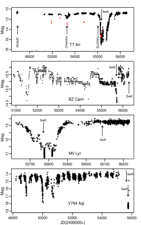
Figure 1: Light curves of TT Ari, BZ Cam, MV Lyr and V794 Aql (from top to bottom) obtained from the AAVSO (crosses), VSNET (filled circles) collaboration and ASAS (open circles) data. The times of the X-ray observations are marked with arrows.

2 Previous optical and UV observations

In Table 1 we report parameters from the published results of observations in the optical, near (NUV) and far (FUV) ultraviolet wavelength ranges. We see that these objects have an orbital period just above the period gap, in a narrow range between 3.2 and 3.7 hours. For the three systems MV Lyr, TT Ari and V794 Aql the WD effective temperature T_eff was estimated in previous low states (not shown in Fig. 1) from UV and FUV observations, in the range between 39,000 K and 47,000 K. These systems could not have been SSS at the time of those observations, because T_eff places the flux peak in the FUV range. On the other hand, we cannot rule out ignition of thermonuclear burning, neither the possibility that the WD may become hotter with time in subsequent low states. The low state T_eff of MV Lyr tabulated in Tab. 1 was measured while the FUV flux, corresponding to most of the bolometric one, was about 3.6 $\times 10^{-12}$ erg s^-1 (see Table 1). In Fig. 5 of Starrfield et al. (2012) we see that at the tabulated distance these values may be consistent with thermonuclear burning with $\dot{m}<1.6\times 10^{-10}$ M_⊙ yr^-1 and a WD mass less than 1 M_⊙. Godon & Sion (2011) suggested that MV Lyr becomes hotter in the high state, hypothesizing a lower limit T${}_{\rm eff}\geq 50,000$ K, consistent with a measured FUV flux of 2.5 $\times 10^{-10}$ erg s^-1 in the high state. If the WD really becomes hotter while emitting X-rays at this level, the possibility of thermonuclear burning would be even more likely in the high state. For a WD mass of 0.7 M_⊙ and the value of $\dot{m}$ in Table 1, assuming that the extreme UV (EUV) luminosity is close to the total (bolometric) luminosity, nuclear burning according to Starrfield et al. (2012) occurs with T${}_{\rm eff}\simeq 80,000$ K (see their Fig. 5), which implies a peak luminosity in the EUV range and no detectable SSS. An accurate determination of T_eff in the high state is important: even an upper limit inferred from the absence of an SSS in the X-rays is useful to constrain the evolutionary models.

Table 1: Binary parameters

	BZ Cam	MV Lyr	TT Ari	V794 Aql
Dist(pc)	$830\pm 160^{[1]}$	$505\pm 50^{[3]}$	$335\pm 50^{[7]}$	$690\pm 105^{[10]}$
P${}_{\rm{orb}}(d)$	$0.1536^{[2]}$	$0.1329^{[4]}$	$0.1375^{[8]}$	$0.1533^{[11]}$
$i^{\rm{o}}$	12–40[1]	10–13[4]	17–22[9]	$60^{[10]}$
MWD(M⊙)		$0.7\pm 0.1_{(FUV)}^{[3]}$	0.57–1.2${}_{(Opt)}^{[9]}$	$0.88\pm 0.39^{[10]}$
$\rm{\dot{m}}_{\rm{High}}$(M⊙ yr-1)		2–3$\times 10^{-9}$(FUV,Opt) [5],[6]	$1.1\times 10^{-8}$(Opt)[9]	10-8.5–10-8.0(FUV)[10]
$\rm{\dot{m}}_{\rm{Low}}$(M⊙ yr-1)		3$\times 10^{-13}$(Opt)[3]	10-16–$10^{-15}$(UV)[7]
T${}_{\rm{WD~{}High}}$		$\geq 50000K_{(FUV)}^{[5]}$
T${}_{\rm{WD~{}Low}}$		$47000K_{(FUV)}^{[3]}$	$39000K_{(UV)}^{[7]}$	$45000K_{(FUV)}^{[10]}$
T${}_{\rm{Disk~{}Low}}$		$<2500K_{(UV)}^{[6]}$
FUV FluxHigh(erg cm-2 s-1)		1.4$\times 10^{-10}$[5]∗	$7.8\times 10^{-10}$[12]∗∗
FUV FluxLow (erg cm-2 s-1)		9.4$\times 10^{-12}$[3]∗∗
Notes:(FUV), (UV), (Opt) – values obtained from Far UV, UV and Optical observations, respectively. ∗ FUV flux was evaluated from the mean continuum level of a spectrum in a rage 910–1190 Å. ∗∗FUV flux was evaluated from the mean continuum level of a spectrum in a rage 920–1180 Å.
[1]Ringwald & Naylor (1998), [2]Patterson et al. (1996), [3]Hoard et al. (2004), [4]Skillman et al. (1995), [5]Godon & Sion (2011), [6]Linnell et al. (2005), [7]Gänsicke et al. (1999), [8]Thorstensen et al. (1985), [9]Belyakov et al. (2010), [10]Godon et al. (2007), [11]Honeycutt & Robertson (1998), [12]Hutchings & Cowley (2007)

3 Observations and data analysis

We examined the archival X-ray data of VY Scl-type stars obtained with Swift, ROSAT, Suzaku and Chandra and chose the objects that were observed both in the high and low states: BZ Cam, MV Lyr, TT Ari and V794 Aql. The data are summarized in Table 2. All the data were never published except for a ROSAT observations of TT Ari, which we examined again and which were also analysed by Baykal et al. (1995) and van Teeseling et al. (1996).

In order to assess when the low and high optical states occurred, we relied on the data of the Variable Star Network (VSNET) Collaboration (Kato et al., 2004) , the American Association of Variable Star Observers (AAVSO) and ASAS databases. The optical light curves are presented in Figure 1. The epoch of the X-ray observation is marked with an arrow in each plot. We did not find optical data for V794 Aql around the epoch of the X-ray observations taken on 15 March 2011. However, from the photometric observations of the object before and after this date presented in Honeycutt et al. (2014) it is reasonable to assume that V794 Aql was in the intermediate state during the X-ray observation.

We used the HEASOFT version 6-13 to extract the Swift and Suzaku spectra, and the XSPEC version 12.8.0 for spectral modelling. We also measured the UV magnitudes of the objects in both the Swift/UVOT observations and in additional GALEX archival exposures. The Chandra ACIS-S+HETG grating spectra were extracted with CIAO version 4.3. Four different partial exposures were added for both the HEG and MEG gratings spectra with the FTOOL ADDASCASPEC, written originally for ASCA, but also useful for all X-ray telescopes and detectors.

For better resolution and in order to use the full exposure, we also combined the data from two Suzaku front illuminated detectors (XIS 0 and XIS 3) taken in 3x3 and 5x5 modes. The timing analysis of the Suzaku data was performed with the XRONOS sub-package of FTOOLS after the barycentric correction.

4 Results

4.1 TT Ari

TT Arietis is one of the brightest CVs, usually between V magnitude 10 and 11. Sometimes it abruptly falls into an ‘intermediate state’ at V$\simeq$14 or even into a ‘low state’ reaching V$\simeq$18. According to Belyakov et al. (2010) this binary system consists of a 0.57–1.2 M_⊙ white dwarf and a 0.18–0.38 M_⊙ secondary component of M 3.5$\pm 0.5$ spectral type (Gänsicke et al., 1999). The only low state before the one discussed in this paper was observed in the years 1980–1985 (Hudec et al., 1984; Shafter et al., 1985). The first panel of Figure 1 shows the long term light-curve of TT Ari between 1990 and 2013. The optical brightness started declining dramatically at the beginning of 2009 and the low state lasted for about 9 months, with a drop in optical luminosity of about 7 mag. However, in the low state the optical luminosity is not constant, with variations between V=15 and V=18.

The high state X-ray spectrum of TT Ari was at first obtained by EXOSAT in Aug 21/22 1985 Hudec et al. (1987). Authors found that the X-ray flux in the range 0.2–4.0 keV was about 1.9$\times 10^{-11}$ erg cm^-2 s^-1. They also proposed that there are two or more hot emitting X-ray regions and two or more cold absorbing or scattering regions in TT Ari. On January 20 to 21, 1994 TT Ari was also observed with ASCA with an effective exposure time $\sim 14,000$ s. Detailed analysis of these data was performed by Baykal & Kiziloğlu (1996). One of the most interesting findings of the previous X-ray observations is the rapid variability of the X-ray flux, a quasi-periodic oscillations (QPO) with a semi-period of 15–26 minutes (Baykal et al. 1995, Baykal & Kiziloğlu 1996). We will show that QPO with periods in this range are observed in all the high state observations we examined. In 2005 the Chandra HETG spectra of TT Ari were obtained by C. Mauche (first shown in a presentation by Mauche, 2010). Below we will discuss this set of observations in details.

Table 2: Observational log of the ROSAT, Swift, Suzaku and Chandra observations of VY Scl-type nova-likes that were analysed in this paper.

Name	State	Date	Instrument	Exposure(s)	Count rate (cts s-1)
BZ Cam	High	21/12/2012	Swift-XRT	15001	$0.0720\pm 0.0024$
	Low	15/05/2011	Swift-XRT	2710	$0.100\pm 0.006$
MV Lyr	High	08/06/2012	Swift-XRT	7569	$0.096\pm 0.003$
	Low	29/07/2011	Swift-XRT	3282	$0.039\pm 0.004$
TT Ari	High	01/08/1991	ROSAT-PSPCB	24464	$0.098\pm 0.007$
	High	06/09/2005	Chandra-HEG	95362∗	$0.0266\pm 0.0003$
	High	06/09/2005	Chandra-MEG	95362∗	$0.0588\pm 0.0005$
	High	06/07/2009	Suzaku-XIS FI∗∗	28617	$0.671\pm 0.003$
	High	06/07/2009	Suzaku-XIS BI∗∗	28617	$0.836\pm 0.005$
	Intermediate	16/10/2009	Swift-XRT	4421	$0.278\pm 0.008$
	Low	22/11/2009	Swift-XRT	12030	$0.0285\pm 0.0019$
V794 Aql	Intermediate	15/03/2011	Swift-XRT	6148	$0.176\pm 0.005$
	Low	12/07/2011	Swift-XRT	4629	$0.055\pm 0.003$
∗Four observations were taken with Chandra-MEG and Chandra-HEG on September 6 and October 4, 6 and 9 2005.
∗∗ Suzaku-XIS FI – are XIS 0 and XIS 3 detectors with front-illuminated (FI) CCDs, while Suzaku-XIS BI is the XIS 1 that utilizes a back-illuminated (BI) CCD

4.1.1 The X-ray data: the high state

A set of four Chandra HETG exposures were obtained within 5 weeks in 2005 (for details see Table 2). In the optical, the source was undergoing a ‘shallow decline’ from the average optical magnitude in the high state, from V$\simeq$10.5 to V$\leq$11.5. Fig. 3 shows the coadded MEG and coadded HEG spectra of four subsequent eposures. There was no significant flux or spectral variability between the different exposures, and we shall describe the coadded MEG and HEG spectra. A rich emission line spectrum was measured, with strong emission lines of Mg, Si, Ne and S.

Figure 2: High state X-ray spectrum of TT Ari taken with ROSAT.

The strongest lines of the Chandra MEG spectrum are listed in Table 3. For the H-like lines we evaluated the flux with a Gaussian fit to the line; we also estimated the flux in the He-like triplet lines (Ne IX, Mg XI, Si XIII), but we could only do it with larger uncertainty because the lines are blended and we needed to fit three Gaussians (note that the intercombination line is not resolved). Moreover, the triplets of He-like lines are observed in a region of the spectrum which is rich in other lines, like those due to transitions of iron. Despite these difficulties, we performed the fit with three Gaussians for the triplets of Si XIII and Mg XI. We added a fourth line of Fe XVIII at 13.509 Å for Ne IX. We thus evaluated the R ratio $f/i$ (intensity of the forbidden to the intercombination line) and the G ratio $(f+i)\over r$ (where r is the intensity of the resonance line). We estimated an uncertainty of about 20% on both these ratios. We obtained R=0.63 and G=0.78 for Ne IX, R=0.36 and G=0.66 for Mg IX, R=0.33 and G=0.66 for Si XIII.

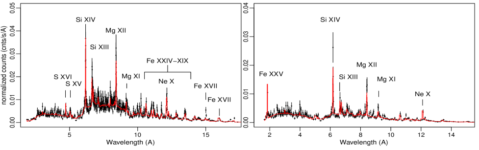
Figure 3: TT Ari spectra observed with the Chandra MEG (left) and HEG (right) grating. Four observations and +1 and -1 orders summed. The red lines represent the fit with two VAPEC components. The emission lines are indicated.

We consulted Porquet & Dubau (2000), who explored the dependence of these ratios on electron density and plasma temperature. The authors assumed a photoionezed plasma, with or without additional collisional ionization. We see from their Figure 8 that the R ratios we obtained corresponds to high density; we obtain a lower limit on the electron density n${}_{\rm e}=10^{12}$ cm^-3, $10^{13}$ cm^-3 and $\geq 10^{14}$ cm^-3 for Ne, Mg and Si, respectively. However, it is known that the R ratios appears smaller, as if the density was higher than its actual value, when there is also photoexcitation by a strong UV/EUV source, exciting the $f$ level electrons into the $i$ level (Porquet & Dubau, 2000). We do expect additional photoexcitation if the lines are produced very close to the hot and luminous WD of TT Ari, thus, we do not know that in this case the R ratio is a completely reliable indicator. The G ratio, on the other hand, is reliable and indicates plasma temperature $\geq 3\times 10^{6}$ K, $\geq 4\times 10^{6}$ K and $\geq 7\times 10^{6}$ for Ne, Mg and Si, respectively.

Figure 4: X-ray light curve of TT Ari, obtained by Suzaku, binned every 100 seconds. The horizontal axis is the orbital phase. The plots are in chronological order.

The next step was to fit the observed spectra with a physical model. A fit with a plasma in collisional ionization equilibrium is not acceptable because of too high $\chi^{2}$, but adding a second temperature we obtained a more reasonable fit, with $\chi^{2}$=1.2. We adopted two BVAPEC models in XSPEC, which describe the emission spectrum of collisionally ionized diffuse gas, calculated using the ATOMDB code v2.0.1 with variable abundances at different temperature (see Table 4 and Fig. 3) and with velocity broadening. By letting the abundances of single elements vary, we found the best fit with the following values for the abundances: [Ne/H]=$6.3\pm 1.2$, [Mg/H]=$4.8\pm 0.8$, [Si/H]=$4.9\pm 0.9$, [S/H]=$11\pm 4$, [Fe/H]=$1.46\pm 0.25$, [O/H]=$10\pm 4$. The emission measure of the cooler component is 3.1$\times 10^{53}$ cm³ and the emission measure of the hotter component is 3.6 $\times 10^{54}$ cm³. We note that, if these two regions are related to accretion, for an electron density of order of 10¹⁴ cm^-3 (the minimum electron density derived from the G ratio for Si), the linear dimension of the emission region is of order of 3.1 $\times 10^{8}$ cm and 7.1 $\times 10^{8}$ cm, respectively. This is, of course, an purely phenomelogical model; two large and distinct regions with different plasma temperature are difficult to explain in a physically realistic way.

Figure 5: Top panel: the Fourier power spectrum of the Suzaku ligh curve of TT Ari. The highest peak corresponds to 0.839 mHz or 19.8 min oscillations. Middle panel: phase folded Suzaku light curve with 19.8 min period. Bottom panel: periods of the QPO and flux in the X-ray range 0.5–10.0 keV in the ROSAT, ASCA, Chandra and Suzaku observations. We assumed the values of Baykal & Kiziloğlu (1996) for the ASCA observations and for the ROSAT X-ray flux. The period of the QPO observed with ROSAT was taken from Baykal et al. (1995).

BVAPEC model performs the Gaussian fitting of the lines and gives the $\sigma$ for two systems of lines associated with the two components (see Table 4). The full width at half maximum that corresponds to these values of $\sigma$ is about 1100 and 1500 km s^-1.

We also wanted to try and better understand the physical scenario by adopting a more physically realistic model. Mukai et al. (2003) have shown that accretion in all non magnetic CVs, and often even in magnetic ones, is best described by a stationary cooling flow model. We thus used the cooling flow VMCFLOW model in XSPEC (a cooling flow model after Mushotzky & Szymkowiak, 1988). We see however that this fit yields a larger $\chi^{2}$ value than the previous simplified model, and this is mainly because there is more flux in the He-like lines than predicted by the model. This may be due to additional photoionization, for instance in a wind from the system, implying that not all the X-ray flux is produced in the accretion flow. The main problem, however, is that the cooling flow model includes the mass accretion rate $\dot{m}$ as a parameter, but predicts a very low value for $\dot{m}$, only $3.48\times 10^{-11}$ M_⊙ yr^-1, while the UV and optical observations indicate $10^{-8}$ M_⊙ yr^-1 for the high state $\dot{m}$ (see Table 1). We thus conclude that either the observed X-ray flux does not originate in the accretion flow that produces the luminous accretion disk, or that accretion energy is mostly re-radiated in the EUV and not in the X-ray range.

Table 3: Measured wavelength and fluxes in erg cm^-2 s^-1 $\times 10^{-14}$ for the emission lines identified in the summed Chandra MEG spectrum.

Element	Energyobs (KeV)	$\lambda_{\rm{obs}}$ ($\rm{\AA}$)	MEG flux${}_{\rm{abs}}^{[1]}$
S XV	2.4606r	5.0387	2.8
	2.448i	5.064	3.3
	2.4260f	5.1106	3.4
Si XIV	2.0061${}_{-0.0010}^{+0.0006}$	6.1803${}_{-0.0017}^{+0.003}$	6.12
Si XIII	1.8650r	6.6479	3.4
	1.854i	6.687	1.7
	1.8396f	6.6739	0.57
Mg XII	1.4733${}_{-0.0011}^{+0.0003}$	8.4154${}_{-0.0020}^{+0.006}$	3.07
Mg XI	1.3522r	9.1687	2.0
	1.3434i	9.2291	1.6
	1.3312f	9.3136	0.59
Ne X	1.0211${}_{-0.0004}^{+0.0007}$	12.142${}_{-0.008}^{+0.005}$	5.25
Ne IX	0.9220r	13.44	3.3
	0.9149i	13.55	1.8
	0.9051f	13.69	0.59
Fe XVIII	0.8735	14.19	0.74
Fe XVII	0.8256${}_{-0.0005}^{+0.0004}$	15.017${}_{-0.008}^{+0.008}$	2.98
Fe XVII	0.7388${}_{-0.0005}^{+0.0006}$	16.781${}_{-0.013}^{+0.014}$	4.8
[1] For a calculation of fluxes in the lines we assumed N(H)=$0.06\times 10^{22}$. r – resonance, i – intercombination and f – forbidden lines.

The light curves of these Chandra exposures still show a QPO, although the modulation has a $\simeq$21 min period. We discuss in detail below the similar light curve we extracted from an additional archival observation done with Suzaku, which has higher S/N.

Suzaku observations of TT Ari were obtained by Saitou in 2009 just before the low state (see top panel of Fig. 1). The average X-ray flux during this observation was higher by almost a factor of 2 than during the Chandra observation. In order to exclude the effect of a slightly different energy ranges of the detectors we compared the X-ray flux in the range 0.5–10.0 keV, common for both instruments. The difference between the X-ray flux measured with Chandra and Suzaku may be correlated with the optical one. The Chandra HETG observations were taken at the time when TT Ari was optically less luminous ($\geq$ 1 mag).

The broad band spectrum of TT Ari observed with Suzaku is presented in Fig. 6. Emission lines of Ne, Mg, Si are clearly seen, like in the Chandra spectrum, together with S, Fe XXV, and Fe XXVI lines. We fit this spectrum either with a two-component thermal plasma model with temperatures 0.80 and 7.1 keV (for details see Table 3) and the abundances that were derived from the Chandra spectra fit. The residuals of the fit indicate an extra line feature at 6.4 keV in the Suzaku spectrum that is most probably the iron fluorescence line. In the inset in Fig. 6 we show the fit of the 5.5–8.0 keV region with three Gaussians at 6.41, 6.68 and 6.96 keV. The equivalent width of the K ${\alpha}$ iron line at 6.41 keV is $96_{-24}^{+24}$ eV. This line implies that the X-ray emission region is close to a ‘cold’ source, which may be the WD surface and/or an optically thick accretion disk, and it is consistent with the WD being less hot than about 100,000 K.

The cooling flow model can be used also for the Suzaku spectrum because we do measure spectral lines to constrain the model. The fit is not optimal, and we run into the same problem of low $\dot{m}$.

The Suzaku light curve is shown in Fig. 4 and is extremely similar to the light curve previously observed with ROSAT (Baykal et al., 1995). The data were integrated in bins of 100 s. The QPO have an amplitude of 50 %. In Fig. 5 we present the Fourier power spectrum of Suzaku light curve of TT Ari. The highest peak corresponds to 0.839 mHz or 19.8 min oscillations. According to Andronov et al. (2009) at the time of Suzaku observations TT Ari also showed QPO in the optical range, with several peaks, at 2.5, 1.1 and 0.38 mHz. In Baykal et al. (1995) the frequency of QPO in X-ray was explained as the beat frequency between the Kepler frequency at the inner edge of the accretion disk and and the star’s rotation rate. Nevertheless, from the QPO semi-periods measured by us in the Chandra and Suzaku observations and from those derived by Baykal et al. (1995) and Baykal & Kiziloğlu (1996), no correlation emerges between the observed frequency of QPO and the X-ray flux of TT Ari (see the bottom panel of Fig. 5).

In 1991 TT Ari was observed with ROSAT. The ROSAT X-ray spectrum is shown in Fig. 2. Baykal et al. (1995) analysed these data and found that the best fitting model is an absorbed black-body. We reanalysed the data and found that a black-body can represent only the soft part of the spectrum (the ROSAT energy range is 0.2–2.4 keV) and for more sophisticated fit we need two-component thermal plasma model. Parameters of the best fitting model are presented in Table 4.

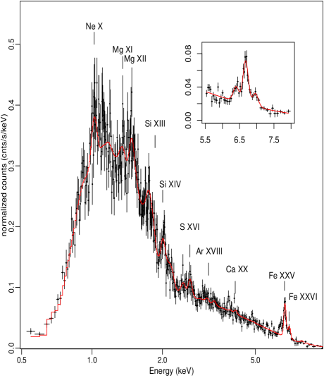
Figure 6: Spectrum observed with the Suzaku XIS FI (data from XIS0 and XIS3 detectors taken in 3x3 and 5x5 modes are summed). The red line shows the fit with two VAPEC components. The emission lines are indicated. The inset show the iron K_α emission lines at 6.41, 6.68 and 6.96 keV and their fit with three Gaussians.

4.1.2 The X-ray data: the low state

In the intermediate and low state TT Ari was observed with Swift. The observations in the intermediate state were presented by Mukai et al. (2009). The unabsorbed flux was about the same as during the Suzaku observation, 1.5 $\times 10^{-11}$ ergs cm^-2 s^-1, the spectrum could only be fitted with a multi-temperature plasma, and a new quasiperiod of 0.4 days was also measured in optical.

The low state spectrum, presented in the top panel of Fig. 8, is best fitted with two components of absorbed thermal plasma in collisional ionization equilibrium with a fixed metallicity APEC model at 0.7 keV and 3.9 keV respectively (we only set a fixed metallicity with solar abundances because of the poorer data quality of this dataset). The low state X-ray flux appeared to be about ten times smaller than in the high and intermediate state, and definitely no luminous supersoft X-ray phase was detected. In Table 4 we show also present the comparison with only one component at 3.4 keV. An upper limit to the temperature of a blackbody-like component is approximately 150,000 K.

Table 4: Fitting models and parameters for TT Ari. The errors represent 90% confidence region for a single parameter.

	high state					low state
Satellite	ROSAT	Chandra		Suzaku		Swift
Models	2 apec	2 bvapec	vmcflow	2 vapec+gauss∗	vmcflow+gauss∗	2 apec	apec
N(H)1($10^{22}$)	$0.0306_{-0.0026}^{+0.003}$	$0.048_{-0.048}^{+0.060}$	$0.026_{-0.015}^{+0.013}$	$0.136_{-0.021}^{+0.022}$	$0.075_{-0.010}^{+0.007}$	$0.04_{-0.04}^{+0.09}$	$0.019_{-0.019}^{+0.05}$
N(H)2($10^{22}$)		$0.121_{-0.029}^{+0.029}$
T1 (keV)	$0.89_{-0.11}^{+0.09}$	$0.93_{-0.03}^{+0.029}$		$0.80_{-0.05}^{+0.13}$		$0.7_{-0.4}^{+0.3}$	$3.4_{-0.7}^{+1.4}$
T2 (keV)	$25_{-13}^{+25}$	$6.5_{-0.4}^{+0.5}$		$7.1_{-0.3}^{+0.3}$		$3.9_{-1.0}^{+2.7}$
Sigma1 ($\rm{kms^{-1}}$)		$646_{-81}^{+81}$
Sigma2 ($\rm{kms^{-1}}$)		$461_{-105}^{+119}$
EM1 ($10^{53}\rm{cm^{-3}}$)∗∗		$3.16_{-0.26}^{+0.43}$
EM2 ($10^{53}\rm{cm^{-3}}$)∗∗		$36.50_{-0.10}^{+0.10}$
Tmin (keV)			$0.20_{-0.026}^{+0.026}$		$0.120_{-0.009}^{+0.016}$
Tmax (keV)			$21.6_{-1.4}^{+1.9}$		$26.9_{-1.5}^{+1.0}$
$\rm{\dot{m}}$ ($\times 10^{-11}\rm{M_{\odot}yr^{-1}}$)			$3.36_{-0.22}^{+0.27}$		$5.02_{-0.11}^{+0.17}$
Flux${}_{\rm{abs}}^{***}$	$5.76_{-0.13}^{+0.3}$	$9.35_{-0.27}^{+0.18}$	$9.01_{-0.3}^{+0.011}$	$15.81_{-0.020}^{+0.020}$	$16.18_{-0.3}^{+0.20}$	$0.99_{-0.18}^{+0.17}$	$0.94_{-0.18}^{+0.17}$
Flux${}_{\rm{unabs}}^{***}$	$6.70_{-0.13}^{+0.3}$	$10.35_{-0.27}^{+0.18}$	$9.21_{-0.3}^{+0.011}$	$17.39_{-0.020}^{+0.020}$	$17.19_{-0.3}^{+0.20}$	$1.08_{-0.18}^{+0.17}$	$1.03_{-0.18}^{+0.17}$
$\chi^{2}$	1.0	1.2	1.6	1.0	1.2	1.0	1.2
∗We added a Gaussian at 6.41 keV in order to fit the K${\alpha}$ iron reflection line in the Suzaku spectrum.
∗∗Emission measure
∗∗∗The X-ray flux ($\times 10^{-12}$erg cm-2 s-1) was calculated in the following energy ranges: 0.2–2.5 keV for ROSAT PSPC, 0.4–10.0 keV for Chandra HETG, 0.5–12.0 keV for Suzaku XIS FI and 0.3–10.0 keV for Swift XRT

4.1.3 UV data

In the first panel of Figure 1, in addition to the optical light curve of TT Ari, the red points show the GALEX near UV (NUV) observations. In Table 6 we give exposure times and the mean AB magnitude in the U/UV filters during the low and high states. The amplitude of the low to high state transition in NUV was much lower than in optical: 3 versus 7 magnitudes. Like in the optical range, TT Ari shows flaring activity in the NUV, with amplitudes up to 1 mag. However, the UV and optical flares occur at different times, and do not appear to correlated, neither anti-correlated. It may be due to the different origine of the UV and optical radiation.

4.2 BZ Cam

BZ Cam shows brightness variations around an average value V = 12–13, with rare occasional transitions to low states with V = 14–14.5. Besides the low state studied here, two additional low states were detected – in 1928 and at the beginning of 2000 (Garnavich & Szkody 1988 and Greiner et al. 2001, respectively). BZ Cam is surrounded by a bright emission nebula with a bow-shock structure, first detected by Ellis et al. (1984) and also studied by Krautter et al. (1987), Hollis et al. (1992), Greiner et al. (2001). Hollis et al. (1992) proposed that the bow shock structure is due to the interactions of the wind of BZ Cam with the interstellar medium. The wind in BZ Cam was also studied by Honeycutt et al. (2013). Greiner et al. (2001) suggested that this nebula is photoionized by a bright central object that must be a super soft X-ray source, while the bow shock structure is due to the high proper motion of BZ Cam, moving while it emits the wind.

4.2.1 X-ray data

The second plot of Fig. 8 shows the X-ray spectra of BZ Cam observed with the Swift XRT. The luminosity is higher in the low state, however, in the very soft spectral region, at energy $\leq$0.5 keV, the X-ray flux is almost twice higher in the high state, which is exactly the opposite of the scenario predicted by Greiner et al. (1999). Interestingly, the spectral fits in both states indicate that we may be observing an unresolved, strong Ne X Lyman ${\alpha}$ line at 1.02 keV. In the high state spectrum the Fe XXV line at 6.7 keV is clearly detected. BZ Cam was also previously observed with ROSAT in the high state. van Teeseling & Verbunt (1994) and Greiner (1998) fitted the spectrum either with one component blackbody or with a highly absorbed bremsstrahlung (or MEWE) model. Greiner (1998) favored the blackbody. However, with the larger energy range of Swift we see that a fit including also the high energy part of the spectrum, is only possible with at least two components, and that the blackbody is not adequate. The black dots in the second panel of Fig. 8 show the low state spectrum of BZ Cam, and a fit with a two-component VAPEC model. With only a broad band spectrum and no detected emission lines, we could not adequately fit the cooling flow model. The same is true for other low resolution X-ray spectra described below.

The high state of BZ Cam (red dots in the second panel of Fig. 8) is best fitted with a two components VAPEC model. The fitting parameters are listed in Table 5. We find the best fit with non solar abundances, [Fe/H]=($4.5\pm 2.4$) and [Ne/H]=($\sim 14$). In the low state, the increased flux seems to be due to a higher maximum temperature, 64 keV instead of about 10 keV. The column density N(H) appears to increase in the low state. Again, a lower limit to the blackbody temperature is of about 150,000 K.

Table 5: Fitting models and parameters for BZ Cam and MV Lyr. The errors represent 90% confidence region for a single parameter.

	BZ Cam			MV Lyr
	high state		low state	high state		low state
Satellite	Swift		Swift	Swift		Swift
Models	vapec	2 vapec	2 apec	vapec+plow	2 apec	2 apec
N(H)($10^{22}$)	$0.14_{-0.03}^{+0.03}$	$0.26_{-0.08}^{+0.12}$	$0.7_{-0.7}^{+0.4}$	$0.24_{-0.24}^{+0.5}$	$0.69_{-0.26}^{+0.16}$	$0.73_{-0.52}^{+0.73}$
Photon Index				$1.00_{-0.24}^{+0.5}$
T1 (keV)	$9.3_{-1.7}^{+0.2.8}$	$0.51_{-0.20}^{+0.3}$	$0.3_{-0.3}^{+0.0.4}$	$0.18_{-0.49}^{+0.38}$	$0.11_{-0.04}^{+0.03}$	$0.12_{-0.05}^{+0.07}$
T2 (keV)		$10.8_{-2.3}^{+4}$	$63.6_{-54}^{+0.4}$		$58_{-50}^{+6}$	$2.47_{-1.6}^{+1.9}$
Fluxabs∗	$3.85_{-0.29}^{+0.24}$	$4.04_{-0.3}^{+0.22}$	$6.4_{-2.2}^{+5}$	$6.5_{-1.6}^{+0.4}$	$6.0_{-6}^{+3.5}$	$1.2_{-0.4}^{+1.3}$
Fluxunabs∗	$4.24_{-0.29}^{+0.24}$	$4.98_{-0.3}^{+0.22}$	$14_{-2.2}^{+5}$	$9.7_{-1.6}^{+0.4}$	$90_{-90}^{+52}$	$75_{-25}^{+81}$
$\chi^{2}$	1.6	1.1	1.0	1.0	1.2
∗The X-ray flux ($\times 10^{-12}$erg cm-2 s-1) for Swift XRT was calculated in the range 0.3–10.0 keV

4.2.2 UV observations

BZ Cam was observed in UV with Swift during the low state with a 1172.43 s exposure and with a 121 s exposure during the high state. The UV magnitudes in the AB system in the high and low states, given in Table 6, indicate a smaller variation than observed in the other objects. This is explained by Figure 7 in which we show the UV image of the nebula obtained with Swift/UVOT observations. Even with the poor spatial resolution of UVOT, we detect an extended object; obviously the ionized nebula also emits copious UV flux. Comparing the image of BZ Cam in Figure 7 and the optical image in Figure 4 of Greiner et al. (2001), we see a trace of the bow shock oriented in the South-slightly South-West direction, but there seems to be additional UV emission of the nebula in the North-East direction, unlike in the in O [III] and H ${\alpha}$ images taken in September of 2000 with the WIYN telescope (Greiner et al., 2001).

Figure 7: Swift UV image of BZ Cam, notice the emission nebula.

Table 6: UV observations

Object	State	Date	Instrument	Exp.(s)	Mag.AB	Filter∗
BZ Cam	High	21/12/2012	Swift UVOT	1200.74	$13.0\pm 1.0$	UVW2
	Low	15/05/2011	Swift UVOT	2737.32	$13.198\pm 0.011$	U
MV Lyr	Low	29/07/2011	Swift UVOT	2092.81	$16.265\pm 0.019$	U
TT Ari	High	01/11/2005	GALEX	1468.3	$12.52\pm 0.001$	FUV
	High	13/11/2003–03/11/2007	GALEX	80–1686	$12.518\pm 0.003$	NUV
	Low	15/11/2009–02/12/2009	GALEX	1466–1702	$15.364\pm 0.003$	NUV
	Low	22/11/2009	Swift UVOT	6311.28	$15.091\pm 0.011$	UVW2
V794 Aql	Intermediate	15/03/2011	Swift UVOT	6186.67	$17.073\pm 0.025$	UVW1
	low	12/07/2011	Swift UVOT	4732.45	$19.26\pm 0.10$	UVM2
Swift filters central wavelengths (Å): U – 3465, UVW1 – 2600, UVM2 – 2246, UVW2 – 1928.
GALEX UV band (Å): NUV – 1750–2800, FUV – 1350–1750

4.3 MV Lyr

MV Lyr spends most of the time in the high state, having brightness in the range V = 12–13, and during the occasional short low states it is in the range V = 16–18. Historical light curves of MV Lyr can be found in Rosino et al. (1993), Wenzel & Fuhrmann (1983), Andronov & Shugarov (1982) and Pavlenko & Shugarov (1998). With their FUSE (Far Ultraviolet Spectroscopic Explorer) observations Hoard et al. (2004) estimated that during the low state $\dot{m}\leq 3\times 10^{-13}$ M_⊙ yr^-1, a four orders of magnitude decrease from the value of $\dot{m}$ estimated by Godon & Sion (2011) in the high state.

4.3.1 X-ray data

The third plot of Figure 8 shows the comparison between the high and low state X-ray spectra of MV Lyr obtained with Swift together with the spectral fits. Unlike in BZ Cam, the high state X-ray flux of MV Lyr is higher by an order of magnitude than in the low state. The spectrum is also harder, with an additional component prominent above 1.7 keV.

We fitted the high state spectrum of MV Lyr with a two components thermal plasma model, but a good fit is also obtained with a thermal plasma and a power law model. We fitted the low S/N, low state spectrum with a two components plasma model with fixed solar abundances, without any attempt to explore the role of the abundances (see Table 5).

A ROSAT observation of MV Lyr in November 1992 in the high state was studied by Greiner (1998). The authors fitted the spectrum with a black body, however, like in the case of BZ Cam, this model fails to fit the high energy part of the spectrum that we measured with Swift. Greiner (1998) observed MV Lyr at the end of the 9 week optical low state in 1996 and obtained only an upper limit for the X-ray luminosity of 10^29.7 erg s^-1 assuming a distance of 320 pc (smaller than the most current estimate of 505$\pm$50 pc we give in Table 1). Assuming a distance of 320 pc, the flux measured during low state observation done with Swift (see Tab. 5) four months after the beginning of the decline to the low state, one month after minimum, would be 10³¹ erg s^-1, more than a factor of 10 higher than this upper limit. Thus, it seems that the X-ray flux of MV Lyr in the low state is not quite constant.

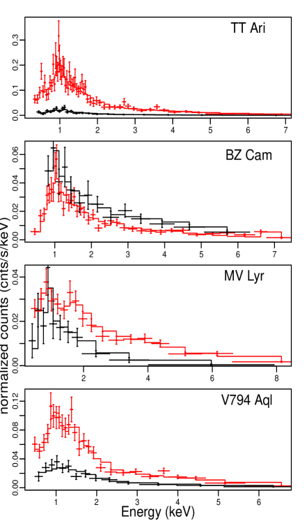
Figure 8: The low and high state X-ray spectra of BZ Cam and MV Lyr observed with Swift. TT Ari and V794 Aql were observed with Swift during the low and intermediate state. The high and intermediate state spectra are plotted in red and the low state spectra in black. The solid lines show the models, the dots with error bars indicate the data.

4.4 V794 Aql

In the high optical state V794 Aql varies between 14th and 15th magnitude, and in the low states it can plunge to 18–20 mag. (in the B filter, see Honeycutt & Schlegel, 1985). Godon et al. (2007) fitted spectra of the Hubble Space Telescope Space Telescope Imaging Spectrograph (HST-STIS) and of FUSE. They derived the following binary system parameters: M${}_{\rm{WD}}=0.9$ M_⊙, high state $\dot{\rm{M}}$ = $10^{-8.5}-10^{-8.0}$ M_⊙ yr^-1, inclination $i=60^{o}$, and distance to the system d = 690 pc.

4.4.1 The X-ray data

The spectra and their fits of V794 Aql in the intermediate state (V$\simeq$15.5) and in the low state are presented in the bottom panel of Fig. 8. The X-ray flux is three times higher in the intermediate than in the low state. We fitted the intermediate state spectrum of V794 Aql with two VAPEC components (see Table 7). In both components we need high abundance of Mg ($\sim 5$). Again, there is no luminous supersoft X-ray source in the low state, with an upper limit of about 150,000 K.

Table 7: Fitting models and parameters for V794 Aql. The errors represent 90% confidence region for a single parameter.

	high state	low state
Satellite	Swift	Swift
Models	2 vapec	apec
N(H)($10^{22}$)	$0.05_{-0.03}^{+0.04}$	$0.005_{-0.05}^{+0.07}$
T1 (keV)	$0.9_{-0.3}^{+0.3}$	$8_{-3}^{+20}$
T2 (keV)	$16_{-8}^{+39}$
Fluxabs∗	$8.2_{-1.3}^{+0.5}\times 10^{-12}$	$2.5_{-0.6}^{+0.4}\times 10^{-12}$
Fluxunabs∗	$8.8_{-1.3}^{+0.5}\times 10^{-12}$	$2.7_{-0.6}^{+0.4}\times 10^{-12}$
$\chi^{2}$	1.0	0.7
∗The X-ray flux ($\times 10^{-12}$erg cm-2 s-1) for Swift XRT was calculated in the range 0.3–10.0 keV

5 Discussion

An important motivation for this research has been the claim by Greiner (1998) and Greiner et al. (2001) that some of the WD in VY Scl-type stars must be burning hydrogen quietly in the low state, without ever triggering thermonuclear flashes because of the short duration of the burning. We found that the predicted supersoft X-ray source does not appear in the low states, so thermonuclear burning at high temperature is ruled out. However, as we see in Table 1 at least 3 of the 4 objects we investigated have low mass M_WD. According to Starrfield et al. (2012) thermonuclear burning in WDs whose mass is lower than 1 M_⊙ occurs quietly with atmospheric temperature below 150,000 K, outside of the SSS window, except for very high values of the mass accretion rate (see Fig.5 of these authors). For Wolf et al. we see that WDs with mass up to 0.7 M_⊙ burn hydrogen in the stable regime (without nova eruptions) with $\dot{m}$ of a few times 10^-7 M_⊙ year^-1 have T${}_{\rm eff}\leq$200,000 K. We note that also CAL 83, hosting a WD burning H at a much higher atmospheric temperature, has low, intermediate and high states in the optical and X-rays, although with a smaller amplitude in the optical than the VY Scl binaries. These variations were associated with the changes in the amount of irradiation of the accretion disc (see e.g. Greiner & Di Stefano 2002, Rajoelimanana et al. 2013).

All the X-ray spectra of the VY Scl systems we examined appear complex, and the Chandra and Suzaku spectra of TT Ari clearly indicate more than one emission region or mechanism. The best-fitting model for all the 0.3–10.0 keV broad band spectra is a, probably still simplistic, two-component absorbed thermal plasma model. Here we discuss the possible origins of the observed X-ray emission.

5.1 Accretion disk boundary layer

We found that in three of the systems the X-ray luminosity decreases during the optical and UV low states, although the X-ray flux variation is the smallest. The X-ray flux seemed to be anti-correlatd with the optical and UV only in BZ Cam. Thus, if in the other three systems the main source of UV/FUV and optical luminosity is the accretion disk, it seems unlikely that the X-ray flux is due to the innermost portion of the disk. In fact, our fits with the cooling flow model, which generally yields good results assuming that all the X-ray flux is emitted in an accretion flow, for all four objects return unreasonably low values of $\dot{m}$, which cannot be reconciled with measurements at other wavelengths. This is not completely unexpected, since the accretion disks of systems accreting at high $\dot{m}$, close to 10^-8 M_⊙ yr^-1, seem to re-radiate mostly or completely in the EUV range (Popham & Narayan, 1995), because the boundary layer is optically thick.

For TT Ari, the semi-regular variability (QPO) with periods of 17–26 minutes in the high state is best explained with the flickering of an accretion disk, however we also found that there is no correlation between the X-ray flux and the frequency of the QPO, which would be expected for accretion disk flickering (Baykal et al. 1995, Popham 1999).

5.2 X-ray emission in a wind

If the origin of the X-ray emission is not in the boundary layer of the accretion disk, it may originate in a wind, either from the WD or from the accretion disk, depleting matter from the system. Such a wind may play an important role in the evolution, preventing the WD from reaching the Chandrasekhar mass. The fit of the TT Ari emission lines observed with Chandra indicates a FWHM in the range 1100–1500 km s^-1. However, the lines do not display any measurable blue or red shift to prove a wind scenario. There is significant broadening, but it may be due to collisional ionization in the accretion flow, or to matter in almost-Keplerian rotation. The WD effective temperature and FUV flux reported in Table 1 are consistent with a line driven wind, although if nuclear burning takes place, the radius of WD at some stage may increase, and we cannot rule out that at some (still not observed) brief stage the WD reaches a luminosity where also electron scattering opacity starts playing a role (a nova-like radiation pressure wind). In either case, the most likely origin for the X-ray flux in the observations we examined is circumstellar material, shocked when it collides with a new outflow, possibly at a large distance from the WD. There may be circumstellar material left from the AGB phase of primary or old remnant of a previous nova, or a previous ‘thicker’ wind caused by enhanced luminosity due to nuclear burning, that has slowed down. A strong stellar wind is very likely to play a role in the extended BZ Cam nebula, which was initially classified as a planetary nebula. Instead we would argue that for TT Ari this explanation cannot account for the largest portion of the X-ray flux, because this system shows a 6.4 keV reflection line, which indicates that a large fraction of X-rays (at least X-rays above 7 keV) must originate close to the white dwarf or to the disk.

There is a secure observation of X-rays far away from the accretion disk in UX UMa (see Pratt et al. 2004), an eclipsing nova-like with a hard, absorbed, eclipsed X-ray component and a soft, unabsorbed, uneclipsed X-ray component. The soft X-rays in UX UMa may indeed originate in a wind from the system. A fast wind is also known to occur in CAL 87 (Greiner et al. 2004, Orio et al. 2004), another system that may be closely related to the VY Scl-type stars. The X-rays and optical flux variations anticorrelate only in BZ Cam, so it is possible that in this system the wind increases in the low state, causing additional absorption and obscuring the accretion disk.

Disk winds are observed in many types of compact objects, while the mechanism that causes them is not completely clear. At optical and UV wavelengths a mass outflow from the disk has been inferred in some CV via the observation P Cygni profiles, most notably the CIV $\lambda$1549 Å line (Robinson 1973, Cordova & Mason 1982, Long & Knigge 2002). P Cygni line profiles or/and absorption features have also been detected in X-rays in low mass X-ray binaries (Ueda et al. 2001, Brandt & Schulz 2000) and are assumed to originate in a high-velocity outflow from a flared and X-ray-heated accretion disk. Disk winds also cause additional circumstellar, sometimes time-dependent, absorption components in the soft X-rays in non-magnetic CV’s (Baskill et al. 2001, Saitou et al. 2012).

5.3 Polar caps

A tempting hypothesis is that, while one component of the X-ray flux is due to a mass outflow from the system, another component originates in a different, and coexistent mode of accretion other than the disk, i.e. a stream to the polar caps. In short, the VY Scl would be intermediate polars (IP’s). This scenario explains the lack of a clear correlation of UV/optical versus X-ray flux variations. As in the model proposed by Hameury & Lasota (2002) the stream to the polar caps still continue, at decreased rate, when the accretion disk is periodically disrupted in the optically low state. In an IP, the disk would emit in optical and UV, but it would be truncated instead of having an X-ray emitting boundary layer, no matter what the value of $\dot{m}$ is.

Mauche (2010) compared spectra of magnetic and non-magnetic CV’s and made a point that division into the two classes is not clear-cut on the basis of the X-ray spectrum alone, because of the large variety of observed X-ray spectra of magnetic CV’s. There is no ‘typical’ spectrum among polars and IP’s. There is evidence for and against the magnetic scenario for TT Ari, but the X-ray spectrum alone does not prove or disprove it.

An X-ray flux modulation due to the WD rotation period, which is very typical and is considerd the smoking gun to classify IP’s, has not been detected in these systems so far. For three of them the reason may be low inclination, but not so for V794 Aql. However, if the major component of the X-ray flux in the high state is not the accretion stream to the poles, but it is associated instead with a wind, isolating the accretion component for the timing analysis is a serious hurdle in detecting a periodicity due to the WD rotation.

6 Conclusions

The VY Scl binaries are critical to understand the evolution of WD interacting binaries. They pose several riddles for the theories and understanding them well is a key to a consistent evolutionary picture. Are these systems almost always quietly accreting at a high rate, with short intervals of low $\dot{m}$ that prevent the occurence of a thermonuclar flash and mass loss in nova outbursts? Is thermonuclear burning of hydrogen on-going at all phases, and how do we find evidence since we do not observe their WD at the high effective temperature necessary to emit supersoft X-rays?

We analyzed a number of X-rays and UV observations of four VY Scl systems comparing phenomena occurring during the optically ‘high’ and ‘low’ state. We did not detect supersoft X-ray emission in both states, however, we cannot exclude H burning at a lower temperature, outside of the SSS window, as can be expected from the low masses of the white dwarfs in these systems. The data collected and examined in this paper suggest that the X-ray emission has more than one component in all the four systems. We concluded that one component most likely originates in the circumstellar material, shocked by the wind, possibly at a large distance from the WD while the second component can be X-ray emission from the polar caps. However, we are not able to prove neither clearly disprove an IP scenario for these systems.

It can be argued that the X-ray observations at this stage have posed more new puzzles. We suggest that monitoring these systems over the years in optical, UV and X-rays as frequently and simultaneously as possible is a key to understand how accretion occurs and how it interplays with the thermal state of the secondary. More intensive monitoring, that may be done with Swift, would be very rewarding, allowing to understand whether an evolutionary path at high mass transfer rate without mass loss in nova outbursts can be sustained for a long time, and whether it leads to ‘quieter’ outflows preventing the WD growth in mass, or to evolution towards a type Ia supernova.

Mauche, C., 2010, http$://cxc.harvard.edu/cdo/accr10/pres/Mauche\_$Chris.pdf

References

- Andronov et al. (2009) Andronov I. L., Baklanov A. V., Liakos A., Niarchos P., 2009, ATEL, 2122
- Andronov & Shugarov (1982) Andronov I. L., Shugarov S. Y., 1982, Astronomicheskij Tsirkulyar, 1218, 3
- Baskill et al. (2001) Baskill D. S., Wheatley P. J., Osborne J. P., 2001, MNRAS, 328, 71
- Baykal et al. (1995) Baykal A., Esendemir A., Kiziloglu Ü., Alpar M. A., Ögelman H., Ercan N., İkis G., 1995, A&A, 299, 421
- Baykal & Kiziloğlu (1996) Baykal A., Kiziloğlu Ü., 1996, Ap&SS, 246, 29
- Belyakov et al. (2010) Belyakov K. V., Suleimanov V. F., Nikolaeva E. A., Borisov N. V., 2010, in Werner K., Rauch T., eds, American Institute of Physics Conference Series Vol. 1273 of American Institute of Physics Conference Series, Modeling of the spectral energy distribution of the cataclysmic variable TT Ari and evaluation of the system parameters. pp 342–345
- Brandt & Schulz (2000) Brandt W. N., Schulz N. S., 2000, ApJ, 544, L123
- Cordova & Mason (1982) Cordova F. A., Mason K. O., 1982, ApJ, 260, 716
- Dhillon (1996) Dhillon V. S., 1996, in Evans A., Wood J. H., eds, IAU Colloq. 158: Cataclysmic Variables and Related Objects Vol. 208 of Astrophysics and Space Science Library, The Nova-like variables. p. 3
- Ellis et al. (1984) Ellis G. L., Grayson E. T., Bond H. E., 1984, PASP, 96, 283
- Gänsicke et al. (1999) Gänsicke B. T., Sion E. M., Beuermann K., Fabian D., Cheng F. H., Krautter J., 1999, A&A, 347, 178
- Garnavich & Szkody (1988) Garnavich P., Szkody P., 1988, PASP, 100, 1522
- Godon & Sion (2011) Godon P., Sion E. M., 2011, PASP, 123, 903
- Godon et al. (2007) Godon P., Sion E. M., Barrett P., Szkody P., 2007, ApJ, 656, 1092
- Greiner (1998) Greiner J., 1998, A&A, 336, 626
- Greiner & Di Stefano (2002) Greiner J., Di Stefano R., 2002, A&A, 387, 944
- Greiner et al. (2004) Greiner J., Iyudin A., Jimenez-Garate M., Burwitz V., Schwarz R., DiStefano R., Schulz N., 2004, in Tovmassian G., Sion E., eds, Revista Mexicana de Astronomia y Astrofisica Conference Series Vol. 20 of Revista Mexicana de Astronomia y Astrofisica, vol. 27, Resonant Scattering and Recombination in CAL 87. pp 18–20
- Greiner et al. (2010) Greiner J., Schwarz R., Tappert C., Mennickent R. E., Reinsch K., Sala G., 2010, Astronomische Nachrichten, 331, 227
- Greiner & Teeseling (1998) Greiner J., Teeseling A., 1998, A&A, 339, L21
- Greiner et al. (2001) Greiner J., Tovmassian G., Orio M., Lehmann H., Chavushyan V., Rau A., Schwarz R., Casalegno R., Scholz R., 2001, A&A, 376, 1031
- Greiner et al. (1999) Greiner J., Tovmassian G. H., di Stefano R., Prestwich A., González-Riestra R., Szentasko L., Chavarría C., 1999, A&A, 343, 183
- Hameury & Lasota (2002) Hameury J.-M., Lasota J., 2002, A&A, 394, 231
- Hameury et al. (1999) Hameury J.-M., Lasota J.-P., Dubus G., 1999, MNRAS, 303, 39
- Hessman (2000) Hessman F. V., 2000, New Astron. Rev., 44, 155
- Hoard et al. (2004) Hoard D. W., Linnell A. P., Szkody P., Fried R. E., Sion E. M., Hubeny I., Wolfe M. A., 2004, ApJ, 604, 346
- Hollis et al. (1992) Hollis J. M., Oliversen R. J., Wagner R. M., Feibelman W. A., 1992, ApJ, 393, 217
- Honeycutt & Kafka (2004) Honeycutt R. K., Kafka S., 2004, AJ, 128, 1279
- Honeycutt et al. (2013) Honeycutt R. K., Kafka S., Robertson J. W., 2013, AJ, p. 45
- Honeycutt & Robertson (1998) Honeycutt R. K., Robertson J. W., 1998, AJ, 116, 1961
- Honeycutt & Schlegel (1985) Honeycutt R. K., Schlegel E. M., 1985, PASP, 97, 1189
- Honeycutt et al. (2014) Honeycutt R. K., Shears J., Kafka S., Robertson J. W., Henden A. A., 2014, AJ, 147, 105
- Hudec et al. (1984) Hudec R., Huth H., Fuhrmann B., 1984, Observatory, 104, 1
- Hudec et al. (1987) Hudec R., Wenzel W., Goetz W., Valníček B., Peřestý R., Richter G. A., Hacke G., Huth H., Mrkos A., Tremko J., 1987, Ap&SS, 131, 697
- Hutchings & Cowley (2007) Hutchings J. B., Cowley A. P., 2007, AJ, 133, 1204
- Kato et al. (2004) Kato T., Uemura M., Ishioka R., Nogami D., Kunjaya C., Baba H., Yamaoka H., 2004, PASJ, 56, S1
- King (1997) King A. R., 1997, MNRAS, 288, 16P
- King & Cannizzo (1998) King A. R., Cannizzo J. K., 1998, ApJ, 499, 348
- Krautter et al. (1987) Krautter J., Radons G., Klaas U., 1987, A&A, 181, 373
- Lasota (1999) Lasota J.-P., 1999, in Mineshige S., Wheeler J. C., eds, Disk Instabilities in Close Binary Systems Disc and secondary irradiation in dwarf and x-ray novae. Universal Academy Press, p. 191
- Leach et al. (1999) Leach R., Hessman F. V., King A. R., Stehle R., Mattei J., 1999, MNRAS, 305, 225
- Linnell et al. (2005) Linnell A. P., Szkody P., Gänsicke B., Long K. S., Sion E. M., Hoard D. W., Hubeny I., 2005, ApJ, 624, 923
- Livio & Pringle (1994) Livio M., Pringle J. E., 1994, ApJ, 427, 956
- Long & Knigge (2002) Long K. S., Knigge C., 2002, ApJ, 579, 725
- Mukai et al. (2003) Mukai K., Kinkhabwala A., Peterson J. R., Kahn S. M., Paerels F., 2003, ApJ, 586, L77
- Mukai et al. (2009) Mukai K., Patterson J., Koff B., Morelle E., Stein W., Oksanen A., 2009, ATEL, 2254
- Mushotzky & Szymkowiak (1988) Mushotzky R. F., Szymkowiak A. E., 1988, in Fabian A. C., ed., NATO ASIC Proc. 229: Cooling Flows in Clusters and Galaxies Einstein Observatory solid state detector observations of cooling flows in clusters of galaxies. pp 53–62
- Orio et al. (2004) Orio M., Ebisawa K., Heise J., Hartmann J., 2004, in Tovmassian G., Sion E., eds, Revista Mexicana de Astronomia y Astrofisica Conference Series Vol. 20 of Revista Mexicana de Astronomia y Astrofisica, vol. 27, A New View of the Supersoft X-Ray Source Cal 87 Observed with XMM-Newton. pp 210–210
- Osaki (2005) Osaki Y., 2005, Proceeding of the Japan Academy, Series B, 81, 291
- Patterson et al. (1996) Patterson J., Patino R., Thorstensen J. R., Harvey D., Skillman D. R., Ringwald F. A., 1996, AJ, 111, 2422
- Pavlenko & Shugarov (1998) Pavlenko E. P., Shugarov S. Y., 1998, Astronomical and Astrophysical Transactions, 15, 89
- Pavlenko & Shugarov (1999) Pavlenko E. P., Shugarov S. Y., 1999, A&A, 343, 909
- Popham (1999) Popham R., 1999, MNRAS, 308, 979
- Popham & Narayan (1995) Popham R., Narayan R., 1995, ApJ, 442, 337
- Porquet & Dubau (2000) Porquet D., Dubau J., 2000, A&AS, 143, 495
- Pratt et al. (2004) Pratt G. W., Mukai K., Hassall B. J. M., Naylor T., Wood J. H., 2004, MNRAS, 348, L49
- Rajoelimanana et al. (2013) Rajoelimanana A. F., Charles P. A., Meintjes P. J., Odendaal A., Udalski A., 2013, MNRAS, 432, 2886
- Ringwald & Naylor (1998) Ringwald F. A., Naylor T., 1998, AJ, 115, 286
- Robinson (1973) Robinson E. L., 1973, ApJ, 186, 347
- Rosino et al. (1993) Rosino L., Romano G., Marziani P., 1993, PASP, 105, 51
- Saitou et al. (2012) Saitou K., Tsujimoto M., Ebisawa K., Ishida M., 2012, PASJ, 64, 88
- Shafter et al. (1985) Shafter A. W., Szkody P., Liebert J., Penning W. R., Bond H. E., Grauer A. D., 1985, ApJ, 290, 707
- Skillman et al. (1995) Skillman D. R., Patterson J., Thorstensen J. R., 1995, PASP, 107, 545
- Smak (1983) Smak J., 1983, ApJ, 272, 234
- Starrfield et al. (2012) Starrfield S., Iliadis C., Timmes F. X., Hix W. R., Arnett W. D., Meakin C., Sparks W. M., 2012, Bulletin of the Astronomical Society of India, 40, 419
- Thorstensen et al. (1985) Thorstensen J. R., Smak J., Hessman F. V., 1985, PASP, 97, 437
- Ueda et al. (2001) Ueda Y., Asai K., Yamaoka K., Dotani T., Inoue H., 2001, ApJ, 556, L87
- van Teeseling et al. (1996) van Teeseling A., Beuermann K., Verbunt F., 1996, A&A, 315, 467
- van Teeseling & Verbunt (1994) van Teeseling A., Verbunt F., 1994, A&A, 292, 519
- Warner (1995) Warner B., 1995, Cataclysmic Variable Stars. (Cambridge: Cambridge University Press)
- Wenzel & Fuhrmann (1983) Wenzel W., Fuhrmann B., 1983, Zentralinstitut fuer Astrophysik Sternwarte Sonneberg Mitteilungen ueber Veraenderliche Sterne, 9, 175
- Wu et al. (1995) Wu K., Wickramasinghe D. T., Warner B., 1995, Publ. Astron. Soc. Aust., 12, 60