Stationary patterns and their selection mechanism of Urban crime models with heterogeneous near–repeat victimization effect

Yu Gu, Qi Wang , Guangzeng Yi
Department of Mathematics
Southwestern University of Finance and Economics
555 Liutai Ave, Wenjiang, Chengdu, Sichuan 611130, China
guyu@2011.swufe.edu.cnqwang@swufe.edu.cn, corresponding author.guangzengyi@2011.swufe.edu.cn
Abstract

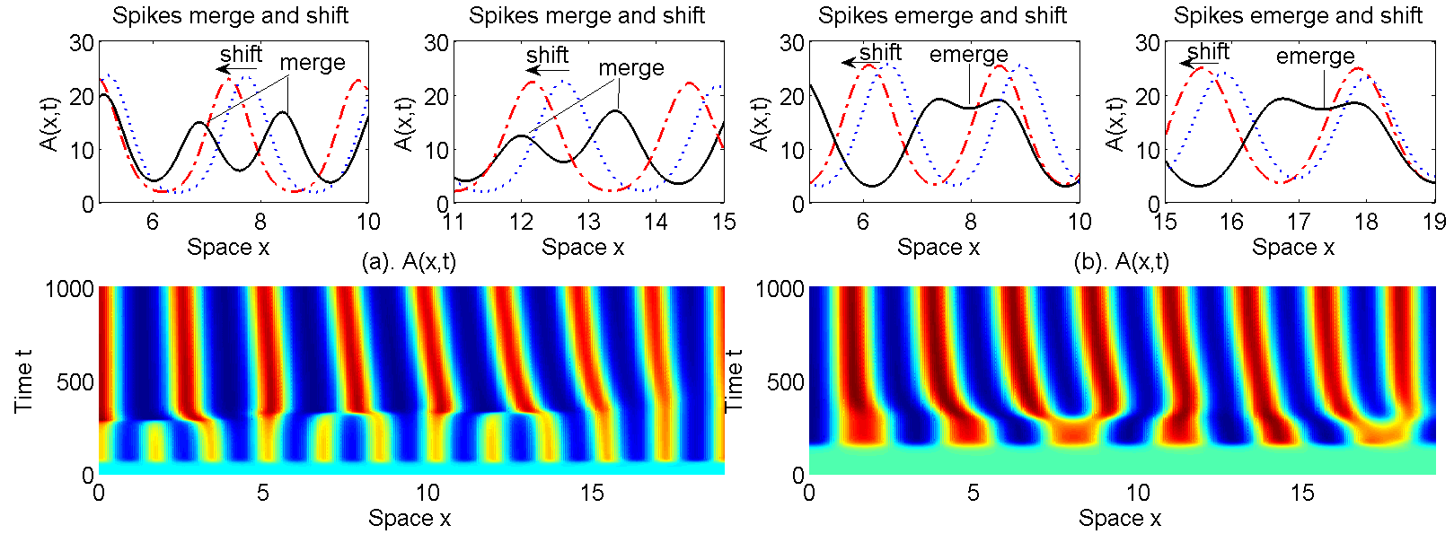
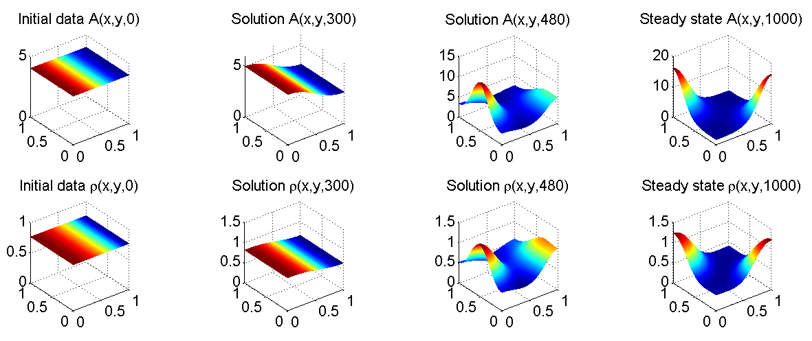
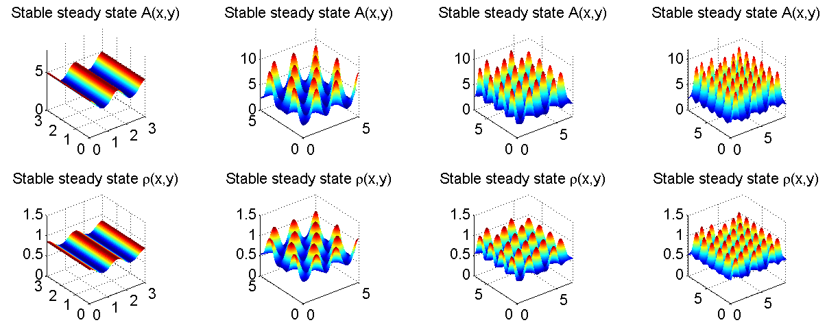
In this paper, we study two PDEs that generalize the urban crime model proposed by Short et al. [Math. Models Methods Appl. Sci., 18 (2008), pp. 1249–1267]. Our modifications are made under assumption of the spatial heterogeneity of both the near–repeat victimization effect and the dispersal strategy of criminal agents. We investigate pattern formations in the reaction–advection–diffusion systems with nonlinear diffusion over multi–dimensional bounded domains subject to homogeneous Neumann boundary conditions. It is shown that the positive homogeneous steady state loses its stability as the intrinsic near–repeat victimization rate ϵitalic-ϵ\epsilon decreases and spatially nonconstant solutions emerge through bifurcation. Moreover, we find the wavemode selection mechanism through rigorous stability analysis of these nontrivial patterns, which shows that the only stable pattern must have wavenumber that maximizes the bifurcation value. Based on this wavemode selection mechanism, we will be able to precisely predict the formation of stable aggregates of the house attractiveness and criminal population density, at least when the diffusion rate ϵitalic-ϵ\epsilon is around the principal bifurcation value. Our theoretical results also suggest that large domains support more stable aggregates than small domains. Finally, we perform extensive numerical simulations over 1D intervals and 2D squares to illustrate and verify our theoretical findings. Our numerics also include some interesting phenomena such as the merging of two interior spikes and the emerging of new spikes, etc. These nontrivial solutions can model the well observed aggregation phenomenon in urban criminal activities.

Keywords: Urban crime model, nonlinear diffusion, pattern formation, stability analysis.

AMS Subject Classification: 35B36, 35J57, 91D25, 65M99

1 Introduction

One of the most noticeable and most often observed phenomena in urban criminal activities is the clustering of crime data. For example, as reported in [4, 5], certain neighbourhoods have a higher propensity to crimes than others though crimes may occur everywhere in the community. Many works in literature are devoted to the understanding of the spatially inhomogeneous distributions of the criminal activities. Great efforts are made to investigate the impact of social forces on such empirical observations and theories proposed for this purpose include social disorganization [27, 33, 38], subculture [6, 47] and conflict theories [9, 11] etc.

It is widely believed that human behaviors are too complex to be explained or predicted individually through mathematical models, however there are regularities of human behaviors that can be modeled and understood mathematically at group level. In the pioneering work of [43], Short et al. proposed mathematical frameworks based on a 2D lattice system and its continuum counterpart to model and simulate the urban residential burglars. The modeling there incorporates an important empirical observation Broken windows effect [39, 46], i.e., a building with a few broken windows which remain unrepaired attracts vandals to break a few more windows and eventually to break the whole building.

In its dimensionless form, the continuum model in [43] is a strongly coupled reaction–advection–diffusion system that reads as follows

{At=ηΔAA+A0+ρA,ρt=(ρ2ρlogA)ρA+B¯,cases𝐴𝑡𝜂Δ𝐴𝐴superscript𝐴0𝜌𝐴missing-subexpression𝜌𝑡𝜌2𝜌𝐴𝜌𝐴¯𝐵missing-subexpression\left\{\begin{array}[]{ll}\frac{\partial A}{\partial t}=\eta\Delta A-A+A^{0}+\rho A,\\ \frac{\partial\rho}{\partial t}=\nabla\cdot(\nabla\rho-2\rho\nabla\log A)-\rho A+\bar{B},\end{array}\right. (1.1)

where (A,ρ)=(A(x,t),ρ(x,t))𝐴𝜌𝐴𝑥𝑡𝜌𝑥𝑡(A,\rho)=(A(x,t),\rho(x,t)) and they denote house attractiveness and criminal population density at space–time location (x,t)𝑥𝑡(x,t) respectively, η𝜂\eta and B¯¯𝐵\bar{B} are positive constants, and A0superscript𝐴0A^{0} is a nonnegative function of x𝑥x. (1.1) is similar as the Keller–Segel models of chemotaxis in which bacteria move along the gradient of the chemical concentration. See the survey papers [15, 19] and [22, 23, 24, 44] for works on the chemotaxis models.

It is demonstrated in [43] that nonlinear system (1.1) and its discrete counterpart can develop very complex spatial–temporal patterns. More interestingly, the pattern formations can qualitatively capture the dynamics of residential burglar aggregates, or the so–called the crime hotspots, presented in the form of spiky steady states. Crime hotspots describe the clustering of crime data in urban residential burglaries, i.e., there are neighbourhoods with higher crime rates surrounded by neighbourhoods with lower crime rates. Moreover, a linear stability has been carried out to determine the parameter values that will lead to the creation of stable hotspots.

In this paper, we investigate the formation of spatially inhomogeneous patterns for following systems with heterogeneous diffusion rate η(A)𝜂𝐴\eta(A) and perception function f(A)𝑓𝐴f(A)

{At=ϵΔ(η(A)(AA0))A+A0+ρA,xΩ,t>0,ρt=(ρ2ρlogf(A))λ0ρA+λ0B¯,xΩ,t>0,cases𝐴𝑡italic-ϵΔ𝜂𝐴𝐴superscript𝐴0𝐴superscript𝐴0𝜌𝐴formulae-sequence𝑥Ω𝑡0𝜌𝑡𝜌2𝜌𝑓𝐴subscript𝜆0𝜌𝐴subscript𝜆0¯𝐵formulae-sequence𝑥Ω𝑡0\left\{\begin{array}[]{ll}\frac{\partial A}{\partial t}=\epsilon\Delta(\eta(A)(A-A^{0}))-A+A^{0}+\rho A,&x\in\Omega,t>0,\\ \frac{\partial\rho}{\partial t}=\nabla\cdot(\nabla\rho-2\rho\nabla\log f(A))-\lambda_{0}\rho A+\lambda_{0}\bar{B},&x\in\Omega,t>0,\end{array}\right. (1.2)

and

{At=ϵ(η2(A)AA0η(A))A+A0+ρA,xΩ,t>0,ρt=(ρ2ρlogf(A))λ0ρA+λ0B¯,xΩ,t>0,cases𝐴𝑡italic-ϵsuperscript𝜂2𝐴𝐴superscript𝐴0𝜂𝐴𝐴superscript𝐴0𝜌𝐴formulae-sequence𝑥Ω𝑡0𝜌𝑡𝜌2𝜌𝑓𝐴subscript𝜆0𝜌𝐴subscript𝜆0¯𝐵formulae-sequence𝑥Ω𝑡0\left\{\begin{array}[]{ll}\frac{\partial A}{\partial t}=\epsilon\nabla\cdot\left(\eta^{2}(A)~{}\nabla\frac{A-A^{0}}{\eta(A)}\right)-A+A^{0}+\rho A,&x\in\Omega,t>0,\\ \frac{\partial\rho}{\partial t}=\nabla\cdot(\nabla\rho-2\rho\nabla\log f(A))-\lambda_{0}\rho A+\lambda_{0}\bar{B},&x\in\Omega,t>0,\end{array}\right. (1.3)

subject to homogeneous Neumann boundary conditions

nA=nρ=0,xΩ,t>0,formulae-sequencesubscriptn𝐴subscriptn𝜌0formulae-sequence𝑥Ω𝑡0\partial_{\textbf{n}}A=\partial_{\textbf{n}}\rho=0,x\in\partial\Omega,t>0, (1.4)

where ΩRNΩsuperscript𝑅𝑁\Omega\subset{R}^{N}, N1𝑁1N\geq 1, is a bounded domain with piecewise smooth boundary ΩΩ\partial\Omega; n is the unit outer normal of the boundary. η(A)𝜂𝐴\eta(A) is a continuously differentiable function satisfying η(A)>0,η(A)>0formulae-sequence𝜂𝐴0superscript𝜂𝐴0\eta(A)>0,\eta^{\prime}(A)>0 and η(A)η(A)A𝜂𝐴superscript𝜂𝐴𝐴\eta(A)\geq\eta^{\prime}(A)A for all A>0𝐴0A>0. f(A)>0𝑓𝐴0f(A)>0 is also assumed to a continuously differentiable function.

The attractiveness A(x,t)𝐴𝑥𝑡A(x,t) consists of two components A(x,t)A0+B(x,t)𝐴𝑥𝑡superscript𝐴0𝐵𝑥𝑡A(x,t)\equiv A^{0}+B(x,t), where A0superscript𝐴0A^{0} represents the static part and B𝐵B measures the dynamic part. Diffusion rate η(A)𝜂𝐴\eta(A) is used to interpret the strength of the empirically observed repeat/near–repeat victimization effect [1, 7, 21], which states that a house and its neighbourhoods become more likely to be burglarized soon after a burglary. f(A)𝑓𝐴f(A) is a function that measures the perception of house attractiveness hence the advection term describes the directed dispersal flux of the criminal agents to the attractive sites over the community with respect to the perception. ϵitalic-ϵ\epsilon is a positive constant that measures the maximum strength of the near–repeat victimization effect and we shall it the intrinsic near–repeat victimization rate. The constants λ0subscript𝜆0\lambda_{0}, A0superscript𝐴0A^{0} and B¯¯𝐵\bar{B} are assumed positive, where λ0subscript𝜆0\lambda_{0} measures the probability that a burglar going back home after committing a crime, A0superscript𝐴0A^{0} and B¯¯𝐵\bar{B} represent the static value and spatial average value of the attractiveness of each house respectively.

The work in [43] has triggered great interest of many scholars in the theoretical analysis and numerical studies of urban crime activities and other similar sociological phenomena. To model the empirically well–observed hotspots from the continuum models, one way is to construct stationary solutions that have concentration structures. In [41], Short et al. performed weak nonlinear analysis based on perturbation arguments to establish the emergence and suppression of stationary hotspot patterns of (1.1). Cantrell et al. [8] applied the local bifurcation theory of Crandall–Rabinowitz [12] and its developed version [40] to investigate the existence and stability of nonconstant positive steady states of (1.1). By Leray–Schauder degree argument, Gacia–Huidobro et al. proved the existence of nonconstant positive steady states to 1D burglar model in [18] and to its general form in [17]. In [26], Kolokolnikov et al. constructed steady state with hotspots and investigated their stabilities when the region is a one–dimensional or two–dimensional domain. Tse and Ward [45] applied a combination of asymptotic analysis and numerical path–following methods to construct hotspot steady states and analyzed their bifurcation properties as the diffusivity of criminals varies. Localized patterns have been studied in [16]. For the time–dependent system (1.1), Rodriǵuez and Bertozzi [36] established the existence and uniqueness of local solutions; Rodriǵuez [35] proved the global existence of fully–parabolic system (1.1) and that of its counterpart with the logarithmic sensitivity logA𝐴\nabla\log A replaced by A𝐴\nabla A, provided that the initial criminal population is small. Berestycki et al. [3] studied a similar system and obtained its traveling wave solutions that connect zones with no criminal activity and zones with crime hotspots.

It is worthwhile to point out that the agent–based model (1.1) in [43] has been extended in several aspects by various authors. For example, effects of police actions on the spatial distribution of criminal activities are taken into account in [20, 34, 41, 49], etc. Chaturapruek et al. [10] proposed a crime model with the criminals following a biased Lévy flight. It is quite difficult for us to list all the works and we refer to [2, 29, 30, 32, 37, 42, 48] and the references therein for the development of models with the same or similar sociological backgrounds. In this paper, we investigate the formation of nonconstant positive steady states to models (1.2) and (1.3) subject to (1.4). We want to remark that the goal of this paper is not to present mathematical models to predict or replicate the behaviors of a single human individuals, but to present a systematic treatment of reaction–advection–diffusion systems modeling urban criminal dynamics, in particular the formation of spatially nontrivial patterns. In particular, all of our theoretical results hold for (1.1) by taking η(A)η𝜂𝐴𝜂\eta(A)\equiv\eta, λ0=1subscript𝜆01\lambda_{0}=1 and f(A)=A𝑓𝐴𝐴f(A)=A in (1.2) or (1.3). On the other hand, we also want to point out that, the nonlinearity in diffusion η(A)𝜂𝐴\eta(A) and perception function f(A)𝑓𝐴f(A), in particular when degeneracy is allowed, can make these models even richer in spatial–temporal dynamics. For example, there are many works on chemotaxis models including but not limited to formation of singularity, compacted supported steady states, etc. We would like to expect more works on the effect of such nonlinearity on the formation and evolution of crime hotspots.

Our paper is organized as follows. In Section 2, we derive the continuum models (1.2) and (1.3) following the microscopic–macroscopic approach in [43]. In Section 3, we carry out the linearized stability analysis of the homogeneous steady state (A¯,ρ¯)¯𝐴¯𝜌(\bar{A},\bar{\rho}) and show that small diffusion rate ϵitalic-ϵ\epsilon tends to destabilize the constant equilibrium–see Proposition 3.1. Section 4 and 5 are devoted to studying the nonconstant positive steady states of (1.2) and (1.3). By Crandall–Rabinowitz bifurcation theory, we rigorously establish the existence and stability of nonconstant steady states–see Theorem 4.1, Theorem 4.2 and Theorem 5.1. We then numerically solve the crime models (1.2) and (1.3) in Section 6 to illustrate the formation of clustering criminal data in the form of hotspots, hotstripes, etc. Finally we include our remarks and propose some future problems in Section 7.

2 Derivation of the models

To understand the relevance of the mathematics presented in [43] and the current work to the urban criminal activities, it is helpful to demonstrate how models (1.2) and (1.3) are derived. We shall extend the urban crime model in [43] to nonlinear diffusion systems (1.2) and (1.3) by considering spatially heterogeneous near–repeat victimization and dispersal strategies of the criminal agents. Moreover, we take into account the nonlinear human perception of a physical stimulus.

2.1 Derivation of the house attractiveness equation

Consider a 2D lattice with constant spacing l𝑙l. Each house is located at site s=(i,j)𝑠𝑖𝑗s=(i,j), i,jN𝑖𝑗𝑁i,j\in{N}, with four neighbouring sites sN(s)={(il,(j±1)l),((i±1)l,jl)}superscript𝑠𝑁𝑠𝑖𝑙plus-or-minus𝑗1𝑙plus-or-minus𝑖1𝑙𝑗𝑙s^{\prime}\in N(s)=\{(il,(j\pm 1)l),((i\pm 1)l,jl)\}. Denote attractiveness of the target house s𝑠s at time t𝑡t by As(t)subscript𝐴𝑠𝑡A_{s}(t) and the number of criminals by ns(t)subscript𝑛𝑠𝑡n_{s}(t) respectively. We want to mention that the attractiveness As(t)subscript𝐴𝑠𝑡A_{s}(t) is defined in a comprehensive way as in [43] and it consists of two part As(t)=A0+Bs(t)subscript𝐴𝑠𝑡subscript𝐴0subscript𝐵𝑠𝑡A_{s}(t)=A_{0}+B_{s}(t), A0subscript𝐴0A_{0} is static and Bssubscript𝐵𝑠B_{s} is dynamic.

According to the near–repeat victimization effect [43], the dynamic attractiveness Bs(t)subscript𝐵superscript𝑠𝑡B_{s^{\prime}}(t) to the neighbouring site of s𝑠s increases each time after it is burglarized, and the increase in Bs(t)subscript𝐵superscript𝑠𝑡B_{s^{\prime}}(t) is contributed by the loss of the attractiveness Bs(t)subscript𝐵𝑠𝑡B_{s}(t) at site s𝑠s, i.e., part of Bs(t)subscript𝐵𝑠𝑡B_{s}(t) is transmitted to its neighbouring sites each time after it is burglarized. This self–exciting phenomenon represents the strong tie of criminal activities to the attractiveness of their environments, as well as the feedback mechanism that local attractiveness is increased by criminal activities. This mechanism is quite similar as the flowing of heat from region of high temperature to regions of low temperature. Here we denote the near–repeat victimization effect by η>0𝜂0\eta>0. Therefore the near–repeat victimization effect is strong if η𝜂\eta is large and it is weak if η𝜂\eta is small. On the other hand, it is very likely that η𝜂\eta may vary from house to house. In this paper, we assume that communities with different attractiveness values have different sensitivities to their local criminal activities, therefore η𝜂\eta at site s𝑠s takes the form ηs(t)=η(As(t),t)subscript𝜂𝑠𝑡𝜂subscript𝐴𝑠𝑡𝑡\eta_{s}(t)=\eta(A_{s}(t),t). Moreover, as the transition probability depends on dynamic attractiveness ηssubscript𝜂𝑠\eta_{s} of the current house (departure point) or ηssubscript𝜂superscript𝑠\eta_{s^{\prime}} of the target house (arrival point), we divide our discussions into the following two cases.

2.1.1 Near-repeat victimization effect η𝜂\eta dependent on attractiveness of departure point

If the near–repeat victimization effect at s𝑠s depends on attractiveness of the departure point s𝑠s, then the transition probability of house attractiveness takes the form

P(ss)=ϵηs(t)z,𝑃𝑠superscript𝑠italic-ϵsubscript𝜂𝑠𝑡𝑧P(s\rightarrow s^{\prime})=\frac{\epsilon\eta_{s}(t)}{z}, (2.1)

where ϵitalic-ϵ\epsilon is a positive constant that measures the maximum value of near–repeat victimization effect, z𝑧z is the number of neighbouring sites of s𝑠s (z=4𝑧4z=4 in 2D) and the notation ss𝑠superscript𝑠s\rightarrow s^{\prime} denotes the shifting of dynamic attractiveness from s𝑠s to ssuperscript𝑠s^{\prime} due to the near–repeat victimization effect.

We assume that burglars occur at site s𝑠s during (t,t+δt)𝑡𝑡𝛿𝑡(t,t+\delta t) following a standard Poisson process with probability Ps(t)=1eAs(t)δtsubscript𝑃𝑠𝑡1superscript𝑒subscript𝐴𝑠𝑡𝛿𝑡P_{s}(t)=1-e^{-A_{s}(t)\delta t}, where As(t)δtsubscript𝐴𝑠𝑡𝛿𝑡A_{s}(t)\delta t is the average number of burglars during (t,t+δt)𝑡𝑡𝛿𝑡(t,t+\delta t). Denote the total population and expected population of criminal agents at s𝑠s by ns(t)subscript𝑛𝑠𝑡n_{s}(t) and Es(t)subscript𝐸𝑠𝑡E_{s}(t) respectively. Since the attractiveness decays to its baseline value at a rate ω𝜔\omega if no criminal activity occurs afterwards, the attractiveness at s𝑠s satisfies the difference equation

Bs(t+δt)=(Bs(t)(1ϵηs(t))+ssP(ss)Bs(t))(1ωδt)+θEs(t)=(Bs(t)(1ϵηs(t))+ssϵηs(t)zBs(t))(1ωδt)+θns(t)Ps(t)=(Bs(t)+l2ϵzΔd(ηs(t)Bs(t)))(1ωδt)+θns(t)Ps(t),subscript𝐵𝑠𝑡𝛿𝑡subscript𝐵𝑠𝑡1italic-ϵsubscript𝜂𝑠𝑡subscriptsimilar-tosuperscript𝑠𝑠𝑃superscript𝑠𝑠subscript𝐵superscript𝑠𝑡1𝜔𝛿𝑡𝜃subscript𝐸𝑠𝑡subscript𝐵𝑠𝑡1italic-ϵsubscript𝜂𝑠𝑡subscriptsimilar-tosuperscript𝑠𝑠italic-ϵsubscript𝜂superscript𝑠𝑡𝑧subscript𝐵superscript𝑠𝑡1𝜔𝛿𝑡𝜃subscript𝑛𝑠𝑡subscript𝑃𝑠𝑡subscript𝐵𝑠𝑡superscript𝑙2italic-ϵ𝑧subscriptΔ𝑑subscript𝜂𝑠𝑡subscript𝐵𝑠𝑡1𝜔𝛿𝑡𝜃subscript𝑛𝑠𝑡subscript𝑃𝑠𝑡\begin{split}B_{s}(t+\delta t)&=\Big{(}B_{s}(t)\big{(}1-\epsilon\eta_{s}(t)\big{)}+\sum\limits_{s^{\prime}\sim s}P(s^{\prime}\rightarrow s)B_{s^{\prime}}(t)\Big{)}(1-\omega\delta t)+\theta E_{s}(t)\\ &=\Big{(}B_{s}(t)(1-\epsilon\eta_{s}(t))+\sum\limits_{s^{\prime}\sim s}\frac{\epsilon\eta_{s^{\prime}}(t)}{z}B_{s^{\prime}}(t)\Big{)}(1-\omega\delta t)+\theta n_{s}(t)P_{s}(t)\\ &=\Big{(}B_{s}(t)+\frac{l^{2}\epsilon}{z}\Delta_{d}(\eta_{s}(t)B_{s}(t))\Big{)}(1-\omega\delta t)+\theta n_{s}(t)P_{s}(t),\end{split} (2.2)

where the notation sssimilar-tosuperscript𝑠𝑠s^{\prime}\sim s indicates all the neighboring sites of s𝑠s, θ𝜃\theta is the increase of attractiveness due to one burglary event and ΔdsubscriptΔ𝑑\Delta_{d} is the discrete spatial Laplacian

ΔdBs(t)=(ssBs(t)zBs(t))/l2.subscriptΔ𝑑subscript𝐵𝑠𝑡subscriptsimilar-tosuperscript𝑠𝑠subscript𝐵superscript𝑠𝑡𝑧subscript𝐵𝑠𝑡superscript𝑙2\Delta_{d}B_{s}(t)=\left(\sum\limits_{s^{\prime}\sim s}B_{s^{\prime}}(t)-zB_{s}(t)\right)\Bigg{/}l^{2}. (2.3)

To derive the continuum PDE, we subtract Bs(t)subscript𝐵𝑠𝑡B_{s}(t) from (2.2) and then divide it by δt𝛿𝑡\delta t. Denote the criminal population density by ρs(t)=ns(t)l2subscript𝜌𝑠𝑡subscript𝑛𝑠𝑡superscript𝑙2\rho_{s}(t)=\frac{n_{s}(t)}{l^{2}}. After sending both δt𝛿𝑡\delta t and l𝑙l to zero and applying the limits as in [43]

limδt0+l2δt=D>0,limδt0+θδt=κ>0,formulae-sequencesubscript𝛿𝑡superscript0superscript𝑙2𝛿𝑡𝐷0subscript𝛿𝑡superscript0𝜃𝛿𝑡𝜅0\lim_{\delta t\rightarrow 0^{+}}\frac{l^{2}}{\delta t}=D>0,~{}\lim_{\delta t\rightarrow 0^{+}}\theta\delta t=\kappa>0,

we collect the following equation of the dynamic attractiveness

Bt=ϵDzΔ(ηB)ωB+κDρA.𝐵𝑡italic-ϵ𝐷𝑧Δ𝜂𝐵𝜔𝐵𝜅𝐷𝜌𝐴\frac{\partial B}{\partial t}=\frac{\epsilon D}{z}\Delta(\eta B)-\omega B+\kappa D\rho A. (2.4)

where Δ=i=1N2xi2Δsuperscriptsubscript𝑖1𝑁superscript2superscriptsubscript𝑥𝑖2\Delta=\sum_{i=1}^{N}\frac{\partial^{2}}{\partial x_{i}^{2}} is the Laplacian in RNsuperscript𝑅𝑁{R}^{N}. See [43] for justifications on the limits.

2.1.2 Near-repeat victimization effect η𝜂\eta dependent on attractiveness of arrival point

If the near–repeat victimization effect η𝜂\eta at s𝑠s depends on its arrival-point ssuperscript𝑠s^{\prime}, we can write the transition probability as

P(ss)=ϵηs(t)z,𝑃𝑠superscript𝑠italic-ϵsubscript𝜂superscript𝑠𝑡𝑧P(s\rightarrow s^{\prime})=\frac{\epsilon\eta_{s^{\prime}}(t)}{z}, (2.5)

where ϵitalic-ϵ\epsilon is defined to the same as for (2.1). Then the discrete equation of attractiveness leads us to

Bs(t+δt)=(Bs(t)(1ssP(ss))+ssP(ss)Bs(t))(1ωδt)+θEs(t)=(Bs(t)(1ssϵηs(t)z)+ssϵηs(t)zBs(t))(1ωδt)+θns(t)Ps(t)=(Bs(t)+ϵl2z(ηs(t)ΔdBs(t)Bs(t)Δdηs(t)))(1ωδt)+θns(t)Ps(t),subscript𝐵𝑠𝑡𝛿𝑡subscript𝐵𝑠𝑡1subscriptsimilar-tosuperscript𝑠𝑠𝑃𝑠superscript𝑠subscriptsimilar-tosuperscript𝑠𝑠𝑃superscript𝑠𝑠subscript𝐵superscript𝑠𝑡1𝜔𝛿𝑡𝜃subscript𝐸𝑠𝑡subscript𝐵𝑠𝑡1subscriptsimilar-tosuperscript𝑠𝑠italic-ϵsubscript𝜂superscript𝑠𝑡𝑧subscriptsimilar-tosuperscript𝑠𝑠italic-ϵsubscript𝜂𝑠𝑡𝑧subscript𝐵superscript𝑠𝑡1𝜔𝛿𝑡𝜃subscript𝑛𝑠𝑡subscript𝑃𝑠𝑡subscript𝐵𝑠𝑡italic-ϵsuperscript𝑙2𝑧subscript𝜂𝑠𝑡subscriptΔ𝑑subscript𝐵𝑠𝑡subscript𝐵𝑠𝑡subscriptΔ𝑑subscript𝜂𝑠𝑡1𝜔𝛿𝑡𝜃subscript𝑛𝑠𝑡subscript𝑃𝑠𝑡\begin{split}B_{s}(t+\delta t)&=\Big{(}B_{s}(t)\big{(}1-\sum_{s^{\prime}\sim s}P(s\rightarrow s^{\prime})\big{)}+\sum\limits_{s^{\prime}\sim s}P(s^{\prime}\rightarrow s)B_{s^{\prime}}(t)\Big{)}(1-\omega\delta t)+\theta E_{s}(t)\\ &=\Big{(}B_{s}(t)\big{(}1-\sum\limits_{s^{\prime}\sim s}\frac{\epsilon\eta_{s^{\prime}}(t)}{z}\big{)}+\sum\limits_{s^{\prime}\sim s}\frac{\epsilon\eta_{s}(t)}{z}B_{s^{\prime}}(t)\Big{)}(1-\omega\delta t)+\theta n_{s}(t)P_{s}(t)\\ &=\Big{(}B_{s}(t)+\frac{\epsilon l^{2}}{z}\big{(}\eta_{s}(t)\Delta_{d}B_{s}(t)-B_{s}(t)\Delta_{d}\eta_{s}(t)\big{)}\Big{)}(1-\omega\delta t)+\theta n_{s}(t)P_{s}(t),\end{split} (2.6)

where again we have used the notation of discrete Laplacian (2.3). By the same microscopic–macroscopic approach that leads to (2.4), we obtain the following PDE

Bt=ϵDz(ηΔBBΔη)ωB+κDρA.𝐵𝑡italic-ϵ𝐷𝑧𝜂Δ𝐵𝐵Δ𝜂𝜔𝐵𝜅𝐷𝜌𝐴\frac{\partial B}{\partial t}=\frac{\epsilon D}{z}\big{(}\eta\Delta B-B\Delta\eta\big{)}-\omega B+\kappa D\rho A. (2.7)

We want to point out that (2.7) can be written into the following divergence form,

Bt=ϵDz(η2Bη)ωB+κDρA.𝐵𝑡italic-ϵ𝐷𝑧superscript𝜂2𝐵𝜂𝜔𝐵𝜅𝐷𝜌𝐴\frac{\partial B}{\partial t}=\frac{\epsilon D}{z}\nabla\cdot\left(\eta^{2}~{}\nabla\frac{B}{\eta}\right)-\omega B+\kappa D\rho A.

Moreover, (2.4) and (2.7) are equivalent if η(A)𝜂𝐴\eta(A) is a constant.

2.2 Derivation of the burglars equation

It is assumed in [43] that burglars must leave site s𝑠s for home after committing a crime at this site and they are removed from this location after time t+δt𝑡𝛿𝑡t+\delta t. In this paper, we consider situations slightly general than [43] and assume that criminal agents will take one of the three dispersal strategies at the next time step: (i) leave site s𝑠s with or without their hunting and then are removed from the system; (ii) stay at the current site; (iii) move to one of the neighbouring sites.

To manifest the dispersal strategies above, we divide criminal agents at site s𝑠s into two groups: those who have committed burglaries during time (tδt,t]𝑡𝛿𝑡𝑡(t-\delta t,t] and those have not. Each group of agents will take one of the three options at the next time step: stay at s𝑠s for further hunting, or move to a neighboring site of s𝑠s, or go back home. Define

λ1(δt):probability that the burglar go home after burgling at s;λ2(δt):probability that the burglar go home without burgling at s.:subscript𝜆1𝛿𝑡probability that the burglar go home after burgling at ssubscript𝜆2𝛿𝑡:probability that the burglar go home without burgling at s\begin{split}&\lambda_{1}(\delta t):\text{probability that the burglar go home after burgling at $s$};\\ &\lambda_{2}(\delta t):\text{probability that the burglar go home without burgling at $s$}.\end{split} (2.8)

It is very likely that the criminal agent who has burglarized at s𝑠s is still motivated for more looting goods at this site after a very short time period, therefore we assume that λ1(δt)λ0(0,1)subscript𝜆1𝛿𝑡subscript𝜆001\lambda_{1}(\delta t)\rightarrow\lambda_{0}\in(0,1) as δt0𝛿𝑡0\delta t\rightarrow 0; on the other hand, the criminal agent who has not burglarized are less likely to return home with nothing collected and to model this we assume that λ2(δt)0subscript𝜆2𝛿𝑡0\lambda_{2}(\delta t)\rightarrow 0 as δt0𝛿𝑡0\delta t\rightarrow 0. For technical reasons, we assume that λ2(δt)=o(δt)subscript𝜆2𝛿𝑡𝑜𝛿𝑡\lambda_{2}(\delta t)=o(\delta t) as δt0𝛿𝑡0\delta t\rightarrow 0 in our coming analysis.

If a criminal agent decides to move to one of the neighbouring sites on the grid, the dispersal is treated as random walk in [43], attracted by each of the neighbouring grids with dispersal probability

qss(t)=As(t)ssAs(t),subscript𝑞𝑠superscript𝑠𝑡subscript𝐴superscript𝑠𝑡subscriptsimilar-tosuperscript𝑠𝑠subscript𝐴superscript𝑠𝑡q_{s\rightarrow s^{\prime}}(t)=\frac{A_{s^{\prime}(t)}}{\sum\limits_{s^{\prime}\sim s}A_{s^{\prime}}(t)},

where ssuperscript𝑠s^{\prime} denotes any neighbouring site of s𝑠s. Our extension of this dispersal strategy is based on the following considerations. First of all, if criminal agents choose to commit another burglar at the current site s𝑠s after burglarizing and if the current site is attractive enough, they would prefer staying for extra hunting than probing the neighbouring sites. That being said, qss(t)subscript𝑞𝑠superscript𝑠𝑡q_{s\rightarrow s^{\prime}}(t) needs to incorporate the information of the attractiveness at site s𝑠s.

Second of all, it is assumed in [43] that a criminal agent responds to the attractiveness As(t)subscript𝐴𝑠𝑡A_{s}(t) linearly, however this is based on the assumption that the agent has perfect information of the attractive As(t)subscript𝐴superscript𝑠𝑡A_{s^{\prime}}(t) of each neighbouring site, which might not be realistic. See the definition of transition probability qss(t)subscript𝑞𝑠superscript𝑠𝑡q_{s\rightarrow s^{\prime}}(t) above. Therefore it is of our interest to put human response to physical stimulus into consideration and we assume that the criminal agent’s perception of the attractiveness Assubscript𝐴𝑠A_{s} is not necessarily a linear function. For the generality of our analysis, we denote f(As)𝑓subscript𝐴𝑠f(A_{s}) as the criminal agents’ perception of the attractiveness of site s𝑠s, where f𝑓f is a nonnegative function such that f(A)0superscript𝑓𝐴0f^{\prime}(A)\geq 0 and f(A)A𝑓𝐴𝐴f(A)\leq A for all A0𝐴0A\geq 0. One typical choice is a logarithmic type function, which resembles the Webner–Fecher’s law on human perception to logarithmic of a physical stimulus. Taking these discussions into account, we have that the dispersal probability of burglars moving from s𝑠s to ssuperscript𝑠s^{\prime} is

qss(t)=f(As,ns)s′′N(s){s}f(As′′,ns′′),subscript𝑞𝑠superscript𝑠𝑡𝑓subscript𝐴superscript𝑠subscript𝑛superscript𝑠subscriptsuperscript𝑠′′𝑁𝑠𝑠𝑓subscript𝐴superscript𝑠′′subscript𝑛superscript𝑠′′q_{s\rightarrow s^{\prime}}(t)=\frac{f(A_{s^{\prime}},n_{s^{\prime}})}{\sum\limits_{s^{\prime\prime}\in N(s)\cup\{s\}}f(A_{s^{\prime\prime}},n_{s^{\prime\prime}})}, (2.9)

and the probability of burglars staying at s𝑠s is

qss(t)=f(As,ns)s′′N(s){s}f(As′′,ns′′),subscript𝑞𝑠𝑠𝑡𝑓subscript𝐴𝑠subscript𝑛𝑠subscriptsuperscript𝑠′′𝑁𝑠𝑠𝑓subscript𝐴superscript𝑠′′subscript𝑛superscript𝑠′′q_{s\rightarrow s}(t)=\frac{f(A_{s},n_{s})}{\sum\limits_{s^{\prime\prime}\in N(s)\cup\{s\}}f(A_{s^{\prime\prime}},n_{s^{\prime\prime}})}, (2.10)

where N(s)𝑁𝑠N(s) denotes the neighbouring sites of s=(i,j)𝑠𝑖𝑗s=(i,j).

We also like to point out that, in practice it is also realistic to assume that the criminal agents move to the neighbouring site ssuperscript𝑠s^{\prime} of the largest perceived attractiveness f(As)𝑓subscript𝐴superscript𝑠f(A_{s^{\prime}}) with probability 1, especially when the difference between attractiveness at ssuperscript𝑠s^{\prime} and that of the rest site is ostensible. For example, it is very likely that criminal agents would surely move to the house that appears more attractive to them (e.g., with fancy cars, nice decoration, swimming pool, etc.) than the rest houses that appear less attractive, without having difficulty in choosing between the neighboring sites (unless the neighbouring sites are almost the same). In this case, a realistic dispersal probability would be

qss(t)={1, if f(As)=maxs′′sf(As′′),0, otherwise.subscript𝑞𝑠superscript𝑠𝑡cases1 if f(As)=maxs′′sf(As′′)0 otherwiseq_{s\rightarrow s^{\prime}}(t)=\left\{\begin{array}[]{ll}1,&\text{ if $f(A_{s^{\prime}})=\max_{s^{{}^{\prime\prime}}\sim s}f(A_{s^{{}^{\prime\prime}}})$},\\ 0,&\text{ otherwise}.\\ \end{array}\right.

For the sake of our analysis we shall assume (2.9)–(2.10) and derive the continuum models (1.2) and (1.3).

Criminal agents at site s𝑠s and time t+δt𝑡𝛿𝑡t+\delta t consist of four types: the agents from site s𝑠s who burglarized at time t𝑡t but stayed there for the next time step, the agents from site s𝑠s who did not burglarize at time t𝑡t and stayed, the agents from neighbouring sites ssuperscript𝑠s^{\prime} who burglarized at time t𝑡t, and those from neighbouring sites ssuperscript𝑠s^{\prime} who did not burglarized at time t𝑡t. Following the arguments in [43] in the modeling of repeat victimization effect, we assume that the agents are created at a constant rate ΓΓ\Gamma during time period of length δt𝛿𝑡\delta t. Therefore the total population of criminal agents at site s𝑠s satisfies the following difference equation

ns(t+δt)=ssf(As,ns)ns(1Ps)(1λ2)s′′N(s){s}f(As′′,ns′′)+f(As,ns)ns(1Ps)(1λ2)s′′N(s){s}f(As′′,ns′′)+ssf(As,ns)nsPs(1λ1)s′′N(s){s}f(As′′,ns′′)+f(As,ns)nsPs(1λ1)s′′N(s){s}f(As′′,ns′′)+Γδtsubscript𝑛𝑠𝑡𝛿𝑡subscriptsimilar-tosuperscript𝑠𝑠𝑓subscript𝐴𝑠subscript𝑛𝑠subscript𝑛superscript𝑠1subscript𝑃superscript𝑠1subscript𝜆2subscriptsuperscript𝑠′′𝑁superscript𝑠superscript𝑠𝑓subscript𝐴superscript𝑠′′subscript𝑛superscript𝑠′′𝑓subscript𝐴𝑠subscript𝑛𝑠subscript𝑛𝑠1subscript𝑃𝑠1subscript𝜆2subscriptsuperscript𝑠′′𝑁𝑠𝑠𝑓subscript𝐴superscript𝑠′′subscript𝑛superscript𝑠′′subscriptsimilar-tosuperscript𝑠𝑠𝑓subscript𝐴𝑠subscript𝑛𝑠subscript𝑛superscript𝑠subscript𝑃superscript𝑠1subscript𝜆1subscriptsuperscript𝑠′′𝑁superscript𝑠superscript𝑠𝑓subscript𝐴superscript𝑠′′subscript𝑛superscript𝑠′′𝑓subscript𝐴𝑠subscript𝑛𝑠subscript𝑛𝑠subscript𝑃𝑠1subscript𝜆1subscriptsuperscript𝑠′′𝑁𝑠𝑠𝑓subscript𝐴superscript𝑠′′subscript𝑛superscript𝑠′′Γ𝛿𝑡\begin{split}n_{s}(t+\delta t)=&\sum\limits_{s^{\prime}\sim s}\frac{f(A_{s},n_{s})n_{s^{\prime}}(1-P_{s^{\prime}})(1-\lambda_{2})}{\sum\limits_{s^{\prime\prime}\in N(s^{\prime})\cup\{s^{\prime}\}}f(A_{s^{\prime\prime}},n_{s^{\prime\prime}})}+\frac{f(A_{s},n_{s})n_{s}(1-P_{s})(1-\lambda_{2})}{\sum\limits_{s^{\prime\prime}\in N(s)\cup\{s\}}f(A_{s^{\prime\prime}},n_{s^{\prime\prime}})}\\ +&\sum\limits_{s^{\prime}\sim s}\frac{f(A_{s},n_{s})n_{s^{\prime}}P_{s^{\prime}}(1-\lambda_{1})}{\sum\limits_{s^{\prime\prime}\in N(s^{\prime})\cup\{s^{\prime}\}}f(A_{s^{\prime\prime}},n_{s^{\prime\prime}})}+\frac{f(A_{s},n_{s})n_{s}P_{s}(1-\lambda_{1})}{\sum\limits_{s^{\prime\prime}\in N(s)\cup\{s\}}f(A_{s^{\prime\prime}},n_{s^{\prime\prime}})}+\Gamma\delta t\end{split} (2.11)

which can be simplified as

ns(t+δt)=ssf(As,ns)(nsPs(1λ1)+ns(1Ps)(1λ2))s′′N(s){s}f(As′′,ns′′)+f(As,ns)(nsPs(1λ1)+ns(1Ps)(1λ2))s′′N(s){s}f(As′′,ns′′)+Γδt=sN(s){s}f(As,ns)(nsPs(1λ1)+ns(1Ps)(1λ2))s′′N(s){s}f(As′′,ns′′)+Γδt.subscript𝑛𝑠𝑡𝛿𝑡subscriptsimilar-tosuperscript𝑠𝑠𝑓subscript𝐴𝑠subscript𝑛𝑠subscript𝑛superscript𝑠subscript𝑃superscript𝑠1subscript𝜆1subscript𝑛superscript𝑠1subscript𝑃superscript𝑠1subscript𝜆2subscriptsuperscript𝑠′′𝑁superscript𝑠superscript𝑠𝑓subscript𝐴superscript𝑠′′subscript𝑛superscript𝑠′′𝑓subscript𝐴𝑠subscript𝑛𝑠subscript𝑛𝑠subscript𝑃𝑠1subscript𝜆1subscript𝑛𝑠1subscript𝑃𝑠1subscript𝜆2subscriptsuperscript𝑠′′𝑁𝑠𝑠𝑓subscript𝐴superscript𝑠′′subscript𝑛superscript𝑠′′Γ𝛿𝑡subscriptsuperscript𝑠𝑁𝑠𝑠𝑓subscript𝐴𝑠subscript𝑛𝑠subscript𝑛superscript𝑠subscript𝑃superscript𝑠1subscript𝜆1subscript𝑛superscript𝑠1subscript𝑃superscript𝑠1subscript𝜆2subscriptsuperscript𝑠′′𝑁superscript𝑠superscript𝑠𝑓subscript𝐴superscript𝑠′′subscript𝑛superscript𝑠′′Γ𝛿𝑡\begin{split}n_{s}(t+\delta t)=&\sum\limits_{s^{\prime}\sim s}\frac{f(A_{s},n_{s})\big{(}n_{s^{\prime}}P_{s^{\prime}}(1-\lambda_{1})+n_{s^{\prime}}(1-P_{s^{\prime}})(1-\lambda_{2})\big{)}}{\sum\limits_{s^{\prime\prime}\in N(s^{\prime})\cup\{s^{\prime}\}}f(A_{s^{\prime\prime}},n_{s^{\prime\prime}})}\\ &+\frac{f(A_{s},n_{s})\big{(}n_{s}P_{s}(1-\lambda_{1})+n_{s}(1-P_{s})(1-\lambda_{2})\big{)}}{\sum\limits_{s^{\prime\prime}\in N(s)\cup\{s\}}f(A_{s^{\prime\prime}},n_{s^{\prime\prime}})}+\Gamma\delta t\\ =&\sum\limits_{s^{\prime}\in N(s)\cup\{s\}}\frac{f(A_{s},n_{s})\big{(}n_{s^{\prime}}P_{s^{\prime}}(1-\lambda_{1})+n_{s^{\prime}}(1-P_{s^{\prime}})(1-\lambda_{2})\big{)}}{\sum\limits_{s^{\prime\prime}\in N(s^{\prime})\cup\{s^{\prime}\}}f(A_{s^{\prime\prime}},n_{s^{\prime\prime}})}+\Gamma\delta t.\end{split} (2.12)

Furthermore, in terms of the discrete spatial Laplacian (2.3), we can further simplify (2.12) as

ns(t+δt)=f(l2ΔdnP(1λ1)+n(1P)(1λ2)l2Δdf+(z+1)f+znP(1λ1)+n(1P)(1λ2)l2Δdf+(z+1)f)+fnP(1λ1)+n(1P)(1λ2)l2Δdf+(z+1)f+Γδt=fl2ΔdnP(1λ1)+n(1P)(1λ2)l2Δdf+(z+1)f+(z+1)fnP(1λ1)+n(1P)(1λ2)l2Δdf+(z+1)f+Γδtsubscript𝑛𝑠𝑡𝛿𝑡𝑓superscript𝑙2subscriptΔ𝑑𝑛𝑃1subscript𝜆1𝑛1𝑃1subscript𝜆2superscript𝑙2subscriptΔ𝑑𝑓𝑧1𝑓𝑧𝑛𝑃1subscript𝜆1𝑛1𝑃1subscript𝜆2superscript𝑙2subscriptΔ𝑑𝑓𝑧1𝑓𝑓𝑛𝑃1subscript𝜆1𝑛1𝑃1subscript𝜆2superscript𝑙2subscriptΔ𝑑𝑓𝑧1𝑓Γ𝛿𝑡𝑓superscript𝑙2subscriptΔ𝑑𝑛𝑃1subscript𝜆1𝑛1𝑃1subscript𝜆2superscript𝑙2subscriptΔ𝑑𝑓𝑧1𝑓𝑧1𝑓𝑛𝑃1subscript𝜆1𝑛1𝑃1subscript𝜆2superscript𝑙2subscriptΔ𝑑𝑓𝑧1𝑓Γ𝛿𝑡\begin{split}n_{s}(t+\delta t)=&f\Big{(}l^{2}\Delta_{d}\frac{nP(1-\lambda_{1})+n(1-P)(1-\lambda_{2})}{l^{2}\Delta_{d}f+(z+1)f}\\ &+z\frac{nP(1-\lambda_{1})+n(1-P)(1-\lambda_{2})}{l^{2}\Delta_{d}f+(z+1)f}\Big{)}\\ &+f\frac{nP(1-\lambda_{1})+n(1-P)(1-\lambda_{2})}{l^{2}\Delta_{d}f+(z+1)f}+\Gamma\delta t\\ =&fl^{2}\Delta_{d}\frac{nP(1-\lambda_{1})+n(1-P)(1-\lambda_{2})}{l^{2}\Delta_{d}f+(z+1)f}\\ &+(z+1)f\frac{nP(1-\lambda_{1})+n(1-P)(1-\lambda_{2})}{l^{2}\Delta_{d}f+(z+1)f}+\Gamma\delta t\\ \end{split} (2.13)

Denoting γ=Γ/δt𝛾Γ𝛿𝑡\gamma=\Gamma/\delta t and l2δtDsuperscript𝑙2𝛿𝑡𝐷\frac{l^{2}}{\delta t}\rightarrow D as δt,l0𝛿𝑡𝑙0\delta t,l\rightarrow 0, we arrive at the continuum equation of criminal population density

ρt=Dz+1(ρ2ρlogf(A))λ0ρA+γ.𝜌𝑡𝐷𝑧1𝜌2𝜌𝑓𝐴subscript𝜆0𝜌𝐴𝛾\frac{\partial\rho}{\partial t}=\frac{D}{z+1}\nabla\cdot(\nabla\rho-2\rho\nabla\log f(A))-\lambda_{0}\rho A+\gamma. (2.14)

We can easily observe in this continuum equation that the criminal agents direct their movements along the gradient of house attractiveness.

2.2.1 Reaction–advection–diffusion systems with heterogeneous diffusion rate

According to the analysis above, we arrive at the following two general systems

{Bt=ϵDzΔ(ηB)ωB+κDρA,ρt=Dz+1(ρ2ρlogf)λ0ρA+γcases𝐵𝑡italic-ϵ𝐷𝑧Δ𝜂𝐵𝜔𝐵𝜅𝐷𝜌𝐴missing-subexpression𝜌𝑡𝐷𝑧1𝜌2𝜌𝑓subscript𝜆0𝜌𝐴𝛾missing-subexpression\left\{\begin{array}[]{ll}\frac{\partial B}{\partial t}=\frac{\epsilon D}{z}\Delta(\eta B)-\omega B+\kappa D\rho A,\\ \frac{\partial\rho}{\partial t}=\frac{D}{z+1}\nabla\cdot(\nabla\rho-2\rho\nabla\log f)-\lambda_{0}\rho A+\gamma\end{array}\right. (2.15)

and

{Bt=ϵDz(η2Bη)ωB+κDρA,ρt=Dz+1(ρ2ρlogf)λ0ρA+γ.cases𝐵𝑡italic-ϵ𝐷𝑧superscript𝜂2𝐵𝜂𝜔𝐵𝜅𝐷𝜌𝐴missing-subexpression𝜌𝑡𝐷𝑧1𝜌2𝜌𝑓subscript𝜆0𝜌𝐴𝛾missing-subexpression\left\{\begin{array}[]{ll}\frac{\partial B}{\partial t}=\frac{\epsilon D}{z}\nabla\cdot\left(\eta^{2}~{}\nabla\frac{B}{\eta}\right)-\omega B+\kappa D\rho A,\\ \frac{\partial\rho}{\partial t}=\frac{D}{z+1}\nabla\cdot(\nabla\rho-2\rho\nabla\log f)-\lambda_{0}\rho A+\gamma.\end{array}\right. (2.16)

Due to transformations

A~=A/ω,ρ~=κDωρ,x~=ω(z+1)Dx,t~=ωt.formulae-sequence~𝐴𝐴𝜔formulae-sequence~𝜌𝜅𝐷𝜔𝜌formulae-sequence~x𝜔𝑧1𝐷x~𝑡𝜔𝑡\tilde{A}=A/\omega,~{}\tilde{\rho}=\frac{\kappa D}{\omega}\rho,~{}\tilde{\textbf{x}}=\sqrt{\frac{\omega(z+1)}{D}}\textbf{x},~{}\tilde{t}=\omega t.

and z+1zη(ωA~)=η~(A~)𝑧1𝑧𝜂𝜔~𝐴~𝜂~𝐴\frac{z+1}{z}\eta(\omega\tilde{A})=\tilde{\eta}(\tilde{A}) and f(ωA~)=f~(A~)𝑓𝜔~𝐴~𝑓~𝐴f(\omega\tilde{A})=\tilde{f}(\tilde{A}), systems (2.15) and (2.16) become (1.2) and (1.3) respectively, where the tildes are dropped there without causing any confusion. It is the goal of our paper to investigate the formation of patterns in (2.15) and (2.16) through models (1.2) and (1.3). In particular, we want to study the qualitative behaviors of stable steady states to these systems that model the crime data clustering phenomenon. Without losing the generality of our analysis, we impose homogeneous Neumann boundary conditions for both systems.

3 Linear stability analysis of homogeneous steady state

We are interested in the formation of positive nonconstant steady states of (1.2) and (1.3) subject to (1.4) with interesting patterns. Our starting point is the stability analysis of the homogeneous steady state

(A¯,ρ¯)=(A0+B¯,B¯A0+B¯).¯𝐴¯𝜌superscript𝐴0¯𝐵¯𝐵superscript𝐴0¯𝐵(\bar{A},\bar{\rho})=\Big{(}A^{0}+\bar{B},\frac{\bar{B}}{A^{0}+\bar{B}}\Big{)}.

Linearizing (1.2) around (A¯,ρ¯)¯𝐴¯𝜌(\bar{A},\bar{\rho}), we have from simple calculations that stability of the homogeneous steady state is determined by the eigenvalues of the following matrix

k=(ϵ(η(A¯)+η(A¯)B¯)σk+ρ¯1A¯2ρ¯f(A¯)f(A¯)σkλ0ρ¯σkλ0A¯),\mathcal{H}_{k}=\left(\begin{array}[]{cc}-\epsilon\left(\eta(\bar{A})+\eta\prime(\bar{A})\bar{B}\right)\sigma_{k}+\bar{\rho}-1&\bar{A}\\ \frac{2\bar{\rho}f^{\prime}(\bar{A})}{f(\bar{A})}\sigma_{k}-\lambda_{0}\bar{\rho}&-\sigma_{k}-\lambda_{0}\bar{A}\\ \end{array}\right), (3.1)

where σ=σk>0𝜎subscript𝜎𝑘0\sigma=\sigma_{k}>0, k=1,2,𝑘12k=1,2,\cdots are the k𝑘k–th eigenvalues of ΔΔ-\Delta on ΩΩ\Omega under the Neumann boundary conditions. It is well known that the Neumann Laplacian has a discrete spectrum of infinitely many non-negative eigenvalues which form a strictly increasing sequence 0=σ0<σ1<σ2<<σk<0subscript𝜎0subscript𝜎1subscript𝜎2subscript𝜎𝑘0=\sigma_{0}<\sigma_{1}<\sigma_{2}<...<\sigma_{k}<...\rightarrow\infty. In the sequel, we assume that σksubscript𝜎𝑘\sigma_{k} is a simple eigenvalue and the eigenfunctions {Φk}k=0superscriptsubscriptsubscriptΦ𝑘𝑘0\{\Phi_{k}\}_{k=0}^{\infty} form a complete orthonormal basis of L2(Ω)superscript𝐿2ΩL^{2}(\Omega) with Φ01|Ω|subscriptΦ01Ω\Phi_{0}\equiv\frac{1}{|\Omega|} and ΩΦk2𝑑x=1subscriptΩsuperscriptsubscriptΦ𝑘2differential-d𝑥1\int_{\Omega}\Phi_{k}^{2}dx=1 for each kR+𝑘superscript𝑅k\in{R}^{+}. We have the instability result in the following proposition.

Proposition 3.1.

Let σksubscript𝜎𝑘\sigma_{k} be the k𝑘k–th Neumann eigenvalue of ΔΔ-\Delta. The constant solution (A¯,ρ¯)¯𝐴¯𝜌(\bar{A},\bar{\rho}) of (1.2) is unstable if and only if

ϵ<maxkN+(2B¯f(A¯)f(A¯)+ρ¯1)σkλ0A¯(η(A¯)+η(A¯)B¯)(σk+λ0A¯)σk.italic-ϵsubscript𝑘superscript𝑁2¯𝐵superscript𝑓¯𝐴𝑓¯𝐴¯𝜌1subscript𝜎𝑘subscript𝜆0¯𝐴𝜂¯𝐴superscript𝜂¯𝐴¯𝐵subscript𝜎𝑘subscript𝜆0¯𝐴subscript𝜎𝑘\epsilon<\max_{k\in{N^{+}}}\frac{\big{(}\frac{2\bar{B}f^{\prime}(\bar{A})}{f(\bar{A})}+\bar{\rho}-1\big{)}\sigma_{k}-\lambda_{0}\bar{A}}{(\eta(\bar{A})+\eta^{\prime}(\bar{A})\bar{B})(\sigma_{k}+\lambda_{0}\bar{A})\sigma_{k}}. (3.2)
Proof.

According to the principle of exchange of stability, see Theorem 5.2 in [14] e.g., (A¯,ρ¯)¯𝐴¯𝜌(\bar{A},\bar{\rho}) is stable if both eigenvalues of each ksubscript𝑘\mathcal{H}_{k} have negative real parts and it is unstable if ksubscript𝑘\mathcal{H}_{k} has an eigenvalue with positive real part for some kN+𝑘superscript𝑁k\in{N}^{+}. The characteristic polynomial of (3.1) takes the form g(ξ)=ξ2+Trξ+Det𝑔𝜉superscript𝜉2Tr𝜉Detg(\xi)=\xi^{2}+\text{Tr}\xi+\text{Det}, where

Tr=ϵ(η(A¯)+η(A¯)B¯)σk+1ρ¯+σk+λ0A¯,\text{Tr}=\epsilon\left(\eta(\bar{A})+\eta\prime(\bar{A})\bar{B}\right)\sigma_{k}+1-\bar{\rho}+\sigma_{k}+\lambda_{0}\bar{A},

and

Det=(ϵ(η(A¯)+η(A¯)B¯)σk+1ρ¯)(σk+λ0A¯)A¯(2ρ¯f(A¯)f(A¯)σkλ0ρ¯).\text{Det}=\left(\epsilon\left(\eta(\bar{A})+\eta\prime(\bar{A})\bar{B}\right)\sigma_{k}+1-\bar{\rho}\right)\left(\sigma_{k}+\lambda_{0}\bar{A}\right)-\bar{A}\Big{(}\frac{2\bar{\rho}f^{\prime}(\bar{A})}{f(\bar{A})}\sigma_{k}-\lambda_{0}\bar{\rho}\Big{)}.

Tr>0Tr0\text{Tr}>0 since ρ¯=B¯A0+B¯<1¯𝜌¯𝐵superscript𝐴0¯𝐵1\bar{\rho}=\frac{\bar{B}}{A^{0}+\bar{B}}<1, therefore g(t)𝑔𝑡g(t) has one positive root if and only if g(0)=Det<0𝑔0Det0g(0)=\text{Det}<0. Then (3.2) follows from straightforward calculations and this finishes the proof of Proposition 3.1. \mathchar 1027\relax

By the same analysis we can prove the instability of the homogeneous steady state with respect to (1.3) as follows.

Corollary 1.

Suppose that η(A¯)>η(A¯)B¯𝜂¯𝐴superscript𝜂¯𝐴¯𝐵\eta(\bar{A})>\eta^{\prime}(\bar{A})\bar{B}. The constant solution (A¯,ρ¯)¯𝐴¯𝜌(\bar{A},\bar{\rho}) of (1.3) is unstable if and only if

ϵ<maxkN+(2B¯f(A¯)f(A¯)+ρ¯1)σkλ0A¯(η(A¯)η(A¯)B¯)(σk+λ0A¯)σk.italic-ϵsubscript𝑘superscript𝑁2¯𝐵superscript𝑓¯𝐴𝑓¯𝐴¯𝜌1subscript𝜎𝑘subscript𝜆0¯𝐴𝜂¯𝐴superscript𝜂¯𝐴¯𝐵subscript𝜎𝑘subscript𝜆0¯𝐴subscript𝜎𝑘\epsilon<\max_{k\in{N^{+}}}\frac{(\frac{2\bar{B}f^{\prime}(\bar{A})}{f(\bar{A})}+\bar{\rho}-1)\sigma_{k}-\lambda_{0}\bar{A}}{(\eta(\bar{A})-\eta^{\prime}(\bar{A})\bar{B})(\sigma_{k}+\lambda_{0}\bar{A})\sigma_{k}}. (3.3)

Our stability analysis above suggests that small intrinsic diffusion rate ϵitalic-ϵ\epsilon destroys the stability of the homogeneous steady state (A¯,ρ¯)¯𝐴¯𝜌(\bar{A},\bar{\rho}) to (1.2) and (1.3). Here ϵitalic-ϵ\epsilon interprets the strength of intrinsic near–repeat victimization effect, therefore when each site is sensitive to burglars the neighbouring sites and the near–repeat victimization effect is strong, clustering of data is not expected in the community. It is assumed that η(A)>0superscript𝜂𝐴0\eta^{\prime}(A)>0 for all A>0𝐴0A>0, i.e., neighbourhood with a larger house attractiveness has stronger near–repeat victimization effect. Comparing (3.2) and (3.3), we see that when ϵitalic-ϵ\epsilon is between the maximum values defined in (3.2) and (3.3), (A¯,ρ¯)¯𝐴¯𝜌(\bar{A},\bar{\rho}) loses its stability in the arrival–dependent model (1.3), while it is still stable in the departure–dependent model (1.2). More detailed are included in Section 6 to discuss the differences between the departure–dependent and arrival–dependent models.

4 Existence of nonconstant positive steady states

In this section, we study the existence of nonconstant positive steady states of (1.2) and (1.3) under (1.4), i.e., nonconstant positive solutions to the following quasi–linear elliptic systems

{ϵΔ(η(A)(AA0))A+A0+ρA=0,xΩ(ρ2ρlogf(A))λ0ρA+λ0B¯=0,xΩA𝐧=ρ𝐧=0,xΩ,casesitalic-ϵΔ𝜂𝐴𝐴superscript𝐴0𝐴superscript𝐴0𝜌𝐴0𝑥Ω𝜌2𝜌𝑓𝐴subscript𝜆0𝜌𝐴subscript𝜆0¯𝐵0𝑥Ω𝐴𝐧𝜌𝐧0𝑥Ω\left\{\begin{array}[]{ll}\epsilon\Delta(\eta(A)(A-A^{0}))-A+A^{0}+\rho A=0,&x\in\Omega\\ \nabla\cdot(\nabla\rho-2\rho\nabla\log f(A))-\lambda_{0}\rho A+\lambda_{0}\bar{B}=0,&x\in\Omega\\ \frac{\partial A}{\partial\mathbf{n}}=\frac{\partial\rho}{\partial\mathbf{n}}=0,&x\in\partial\Omega,\end{array}\right. (4.1)

and

{ϵ(η2(A)AA0η(A))A+A0+ρA=0,xΩ,(ρ2ρlogf(A))λ0ρA+λ0B¯=0,xΩ,A𝐧=ρ𝐧=0,xΩ.casesitalic-ϵsuperscript𝜂2𝐴𝐴superscript𝐴0𝜂𝐴𝐴superscript𝐴0𝜌𝐴0𝑥Ω𝜌2𝜌𝑓𝐴subscript𝜆0𝜌𝐴subscript𝜆0¯𝐵0𝑥Ω𝐴𝐧𝜌𝐧0𝑥Ω\left\{\begin{array}[]{ll}\epsilon\nabla\cdot\left(\eta^{2}(A)~{}\nabla\frac{A-A^{0}}{\eta(A)}\right)-A+A^{0}+\rho A=0,&x\in\Omega,\\ \nabla\cdot(\nabla\rho-2\rho\nabla\log f(A))-\lambda_{0}\rho A+\lambda_{0}\bar{B}=0,&x\in\Omega,\\ \frac{\partial A}{\partial\mathbf{n}}=\frac{\partial\rho}{\partial\mathbf{n}}=0,&x\in\partial\Omega.\end{array}\right. (4.2)

We shall perform rigorous bifurcation analysis due to Crandall–Rabinowitz [12] to establish nonconstant positive solutions for (4.1), while the same analysis can be carried out for (4.2). Taking ϵitalic-ϵ\epsilon as the bifurcation parameter, we introduce the operator

=(ϵΔ(η(A)(AA0))A+A0+ρA(ρ2ρlogf(A))λ0ρA+λ0B¯)italic-ϵΔ𝜂𝐴𝐴superscript𝐴0𝐴superscript𝐴0𝜌𝐴missing-subexpression𝜌2𝜌𝑓𝐴subscript𝜆0𝜌𝐴subscript𝜆0¯𝐵missing-subexpression\mathcal{F}=\left(\begin{array}[]{ll}\epsilon\Delta(\eta(A)(A-A^{0}))-A+A^{0}+\rho A\\ \nabla\cdot(\nabla\rho-2\rho\nabla\log f(A))-\lambda_{0}\rho A+\lambda_{0}\bar{B}\\ \end{array}\right) (4.3)

from 𝒳×𝒳×R+𝒳𝒳superscript𝑅\mathcal{\mathcal{X}}\times\mathcal{\mathcal{X}}\times{R}^{+} to 𝒴×𝒴𝒴𝒴\mathcal{Y}\times\mathcal{Y}, where 𝒳𝒳\mathcal{X} is Sobolev space 𝒳={wW2,p(Ω)|w𝐧=0,xΩ}𝒳conditional-set𝑤superscript𝑊2𝑝Ωformulae-sequence𝑤𝐧0𝑥Ω\mathcal{X}=\{w\in W^{2,p}(\Omega)\big{|}\frac{\partial w}{\partial\mathbf{n}}=0,x\in\partial\Omega\} and 𝒴=Lp(Ω)𝒴superscript𝐿𝑝Ω\mathcal{Y}=L^{p}(\Omega) for some p>N𝑝𝑁p>N. We want to point out that here the boundary condition makes sense since W2,p(Ω)C1+α(Ω¯)superscript𝑊2𝑝Ωsuperscript𝐶1𝛼¯ΩW^{2,p}(\Omega)\hookrightarrow C^{1+\alpha}(\bar{\Omega}) for some α>0𝛼0\alpha>0 if p>N𝑝𝑁p>N. (4.1) is equivalent to (A,ρ,ϵ)=0𝐴𝜌italic-ϵ0\mathcal{F}(A,\rho,\epsilon)=0 for (A,ρ,ϵ)𝒳×𝒳×R+𝐴𝜌italic-ϵ𝒳𝒳superscript𝑅(A,\rho,\epsilon)\in\mathcal{X}\times\mathcal{X}\times{R}^{+}. It is easy to see that \mathcal{F} is a continuously differentiable mapping from 𝒳×𝒳×R+𝒳𝒳superscript𝑅\mathcal{X}\times\mathcal{X}\times{R}^{+} to 𝒴×𝒴𝒴𝒴\mathcal{Y}\times\mathcal{Y} and (A¯,ρ¯,ϵ)=0¯𝐴¯𝜌italic-ϵ0\mathcal{F}(\bar{A},\bar{\rho},\epsilon)=0 for any ϵR+italic-ϵsuperscript𝑅\epsilon\in{R}^{+}; moreover, for any fixed (A^,ρ^)𝒳×𝒳^𝐴^𝜌𝒳𝒳(\hat{A},\hat{\rho})\in\mathcal{X}\times\mathcal{X}, the Fréchet derivative of \mathcal{F} is given by

D(A,ρ)(A^,ρ^,ϵ)(A,ρ)=(ϵΔ((η(A^)+η(A^)(A^A0))A)+(ρ^1)A+A^ρ(ρ2ρ^f(A^)f(A^)A+2ρ^f(A^)f(A^)f2(A^)A2ρ^f(A^)f(A^)A2ρf(A^)f(A^))λ0A^ρλ0ρ^A);D_{(A,\rho)}\mathcal{F}(\hat{A},\hat{\rho},\epsilon)(A,\rho)=\left(\begin{array}[]{cc}\vspace{0.2in}\epsilon\Delta((\eta(\hat{A})+\eta^{\prime}(\hat{A})(\hat{A}-A^{0}))A)+(\hat{\rho}-1)A+\hat{A}\rho\\ \nabla\cdot\big{(}\nabla\rho-\frac{2\hat{\rho}f^{\prime}(\hat{A})}{f(\hat{A})}\nabla A+\frac{2\hat{\rho}f^{\prime}(\hat{A})\nabla f(\hat{A})}{f^{2}(\hat{A})}A-\frac{2\hat{\rho}\nabla f^{\prime}(\hat{A})}{f(\hat{A})}A\\ -\frac{2\rho}{f(\hat{A})}\nabla f(\hat{A})\big{)}-\lambda_{0}\hat{A}\rho-\lambda_{0}\hat{\rho}A\end{array}\right); (4.4)

furthermore, by rewriting (4.4) as

D(A,ρ)(A^,ρ^,ϵ)(A,ρ)=I1(ΔAΔρ)+I2(Aρ)+I3(Aρ),subscript𝐷𝐴𝜌^𝐴^𝜌italic-ϵ𝐴𝜌subscript𝐼1Δ𝐴missing-subexpressionΔ𝜌missing-subexpressionsubscript𝐼2𝐴missing-subexpression𝜌missing-subexpressionsubscript𝐼3𝐴missing-subexpression𝜌missing-subexpressionD_{(A,\rho)}\mathcal{F}(\hat{A},\hat{\rho},\epsilon)(A,\rho)=I_{1}\left(\begin{array}[]{ll}\Delta A\\ \Delta\rho\end{array}\right)+I_{2}\left(\begin{array}[]{ll}\nabla A\\ \nabla\rho\end{array}\right)+I_{3}\left(\begin{array}[]{ll}A\\ \rho\end{array}\right),

with

I1=(ϵ(η(A^)+η(A^)(A^A0))02ρ^f(A^)f(A^)1),I_{1}=\left(\begin{array}[]{cc}\epsilon\left(\eta(\hat{A})+\eta\prime(\hat{A})(\hat{A}-A^{0})\right)&~{}~{}~{}~{}0{}{}{}\\ -\frac{2\hat{\rho}f^{\prime}(\hat{A})}{f(\hat{A})}&~{}~{}~{}~{}1{}{}{}\\ \end{array}\right),
I2=(2ϵ(η(A^)+η(A^)(A^A0))02ρ^f(A^)f(A^)f2(A^)2ρ^f(A^)f(A^)2ρ^f(A^)f(A^)2f(A^)f(A^)),I_{2}=\left(\begin{array}[]{cc}2\epsilon\nabla(\eta(\hat{A})+\eta\prime(\hat{A})(\hat{A}-A^{0}))&~{}~{}~{}0{}{}{}\\ \frac{2\hat{\rho}f^{\prime}(\hat{A})\nabla f(\hat{A})}{f^{2}(\hat{A})}-\frac{2\hat{\rho}\nabla f^{\prime}(\hat{A})}{f(\hat{A})}-\nabla\frac{2\hat{\rho}f^{\prime}(\hat{A})}{f(\hat{A})}&~{}~{}~{}\frac{-2\nabla f(\hat{A})}{f(\hat{A})}{}{}{}\\ \end{array}\right),
I3=(ϵΔ(η(A^)+η(A^)(A^A0))+ρ^1A^(2ρ^f(A^)f(A^)f2(A^)2ρ^f(A^)f(A^))λ0ρ^2f(A^)f(A^)λ0A^),I_{3}=\left(\begin{array}[]{cc}\epsilon\Delta(\eta(\hat{A})+\eta\prime(\hat{A})(\hat{A}-A^{0}))+\hat{\rho}-1&~{}~{}~{}\hat{A}\\ \nabla\cdot(\frac{2\hat{\rho}f^{\prime}(\hat{A})\nabla f(\hat{A})}{f^{2}(\hat{A})}-\frac{2\hat{\rho}\nabla f^{\prime}(\hat{A})}{f(\hat{A})})-\lambda_{0}\hat{\rho}&~{}~{}~{}-2\nabla\cdot\frac{\nabla f(\hat{A})}{f(\hat{A})}-\lambda_{0}\hat{A}\\ \end{array}\right),

we see that (4.4) is a linear and compact operator according to standard elliptic regularity and Sobolev embeddings. On the other hand, matrix I1subscript𝐼1I_{1}, defining the principal part of D(A,ρ)(A^,ρ^,ϵ)subscript𝐷𝐴𝜌^𝐴^𝜌italic-ϵD_{(A,\rho)}\mathcal{F}(\hat{A},\hat{\rho},\epsilon), has two positive eigenvalues, therefore D(A,ρ)(A^,ρ^,ϵ)subscript𝐷𝐴𝜌^𝐴^𝜌italic-ϵD_{(A,\rho)}\mathcal{F}(\hat{A},\hat{\rho},\epsilon) is a Fredholm operator with 0 index by Corollary 2.11 or Remark 3.4 of theorem 3.3 in Shi and Wang [43].

The necessary condition for bifurcation at (A¯,ρ¯)¯𝐴¯𝜌(\bar{A},\bar{\rho}) is 𝒩(D(A,ρ)(A¯,ρ¯,ϵ)){(0,0)}𝒩subscript𝐷𝐴𝜌¯𝐴¯𝜌italic-ϵ00\mathcal{N}\left(D_{(A,\rho)}\mathcal{F}(\bar{A},\bar{\rho},\epsilon)\right)\neq\{(0,0)\}, where 𝒩𝒩\mathcal{N} denotes the null set and

D(A,ρ)(A¯,ρ¯,ϵ)(A,ρ)=(ϵ(η(A¯)+η(A¯)B¯)ΔA+(ρ¯1)A+A¯ρΔρ2ρ¯f(A¯)f(A¯)ΔAλ0A¯ρλ0ρ¯A).subscript𝐷𝐴𝜌¯𝐴¯𝜌italic-ϵ𝐴𝜌italic-ϵ𝜂¯𝐴superscript𝜂¯𝐴¯𝐵Δ𝐴¯𝜌1𝐴¯𝐴𝜌missing-subexpressionΔ𝜌2¯𝜌superscript𝑓¯𝐴𝑓¯𝐴Δ𝐴subscript𝜆0¯𝐴𝜌subscript𝜆0¯𝜌𝐴missing-subexpressionD_{(A,\rho)}\mathcal{F}(\bar{A},\bar{\rho},\epsilon)(A,\rho)=\left(\begin{array}[]{ll}\epsilon(\eta(\bar{A})+\eta^{\prime}(\bar{A})\bar{B})\Delta A+(\bar{\rho}-1)A+\bar{A}\rho\\ ~{}~{}~{}\Delta\rho-\frac{2\bar{\rho}f^{\prime}(\bar{A})}{f(\bar{A})}\Delta A-\lambda_{0}\bar{A}\rho-\lambda_{0}\bar{\rho}A\end{array}\right). (4.5)

To show this condition, we choose some (A,ρ)D(A,ρ)(A¯,ρ¯,ϵ)𝐴𝜌subscript𝐷𝐴𝜌¯𝐴¯𝜌italic-ϵ(A,\rho)\in D_{(A,\rho)}\mathcal{F}(\bar{A},\bar{\rho},\epsilon) and substituting their eigen-expansions A=k=0SkΦk(x),ρ=k=0TkΦk(x)formulae-sequence𝐴superscriptsubscript𝑘0subscript𝑆𝑘subscriptΦ𝑘𝑥𝜌superscriptsubscript𝑘0subscript𝑇𝑘subscriptΦ𝑘𝑥A=\sum_{k=0}^{\infty}S_{k}\Phi_{k}(x),\rho=\sum_{k=0}^{\infty}T_{k}\Phi_{k}(x) into (4.5) to collect

(ϵ(η(A¯)+η(A¯)B¯)σk+ρ¯1A¯2ρ¯f(A¯)f(A¯)σkλ0ρ¯σkλ0A¯)(SkTk)=0,\left(\begin{array}[]{cc}-\epsilon(\eta(\bar{A})+\eta\prime(\bar{A})\bar{B})\sigma_{k}+\bar{\rho}-1&\bar{A}\\ \frac{2\bar{\rho}f^{\prime}(\bar{A})}{f(\bar{A})}\sigma_{k}-\lambda_{0}\bar{\rho}&-\sigma_{k}-\lambda_{0}\bar{A}\\ \end{array}\right)\left(\begin{array}[]{cc}S_{k}\\ T_{k}\end{array}\right)=0, (4.6)

then for each kR+𝑘superscript𝑅k\in{R}^{+}, (4.6) has nontrivial solutions if and only if the coefficient matrix is singular, i.e.,

ϵ=ϵ¯k=(2B¯f(A¯)f(A¯)+ρ¯1)σkλ0A¯(η(A¯)+η(A¯)B¯)(σk+λ0A¯)σk,kN+,formulae-sequenceitalic-ϵsubscript¯italic-ϵ𝑘2¯𝐵superscript𝑓¯𝐴𝑓¯𝐴¯𝜌1subscript𝜎𝑘subscript𝜆0¯𝐴𝜂¯𝐴superscript𝜂¯𝐴¯𝐵subscript𝜎𝑘subscript𝜆0¯𝐴subscript𝜎𝑘𝑘superscript𝑁\epsilon=\bar{\epsilon}_{k}=\frac{\big{(}\frac{2\bar{B}f^{\prime}(\bar{A})}{f(\bar{A})}+\bar{\rho}-1\big{)}\sigma_{k}-\lambda_{0}\bar{A}}{(\eta(\bar{A})+\eta^{\prime}(\bar{A})\bar{B})(\sigma_{k}+\lambda_{0}\bar{A})\sigma_{k}},~{}k\in{N}^{+}, (4.7)

and this is the necessary condition for bifurcations to occur at (A¯,ρ¯)¯𝐴¯𝜌(\bar{A},\bar{\rho}). If the eigenvalue σksubscript𝜎𝑘\sigma_{k} is simple, it follows that 𝒩(D(A,ρ)(A¯,ρ¯,ϵ¯k))𝒩subscript𝐷𝐴𝜌¯𝐴¯𝜌subscript¯italic-ϵ𝑘\mathcal{N}(D_{(A,\rho)}\mathcal{F}(\bar{A},\bar{\rho},\bar{\epsilon}_{k})) is one–dimensional and its basis is spanned by {(A¯k,ρ¯k)}subscript¯𝐴𝑘subscript¯𝜌𝑘\left\{(\bar{A}_{k},\bar{\rho}_{k})\right\} with

A¯k=QkΦk,ρ¯k=Φk,formulae-sequencesubscript¯𝐴𝑘subscript𝑄𝑘subscriptΦ𝑘subscript¯𝜌𝑘subscriptΦ𝑘\bar{A}_{k}=Q_{k}\Phi_{k},~{}\bar{\rho}_{k}=\Phi_{k}, (4.8)

where ΦksubscriptΦ𝑘\Phi_{k} is the k𝑘k–th Neumann Laplacian eigenfunction and

Qk=σk+λ0A¯2ρ¯f(A¯)f(A¯)σkλ0ρ¯,kN+.formulae-sequencesubscript𝑄𝑘subscript𝜎𝑘subscript𝜆0¯𝐴2¯𝜌superscript𝑓¯𝐴𝑓¯𝐴subscript𝜎𝑘subscript𝜆0¯𝜌𝑘superscript𝑁Q_{k}=\frac{\sigma_{k}+\lambda_{0}\bar{A}}{\frac{2\bar{\rho}f^{\prime}(\bar{A})}{f(\bar{A})}\sigma_{k}-\lambda_{0}\bar{\rho}},k\in{N}^{+}. (4.9)

The fact that D(A,ρ)(A¯,ρ¯,ϵ)subscript𝐷𝐴𝜌¯𝐴¯𝜌italic-ϵD_{(A,\rho)}\mathcal{F}(\bar{A},\bar{\rho},\epsilon) is Fredholm with index 0 implies that dim 𝒩(D(A,ρ)(A¯,ρ¯,ϵ))𝒩subscript𝐷𝐴𝜌¯𝐴¯𝜌italic-ϵ\mathcal{N}(D_{(A,\rho)}\mathcal{F}(\bar{A},\bar{\rho},\epsilon)) equals codim (D(A,ρ)(A¯,ρ¯,ϵ))=1subscript𝐷𝐴𝜌¯𝐴¯𝜌italic-ϵ1\mathcal{R}(D_{(A,\rho)}\mathcal{F}(\bar{A},\bar{\rho},\epsilon))=1.

We now verify that local bifurcation does occur at (A¯,ρ¯,ϵ¯k)¯𝐴¯𝜌subscript¯italic-ϵ𝑘(\bar{A},\bar{\rho},\bar{\epsilon}_{k}) in the following theorem, which establishes nonconstant positive solutions to (4.1).

Theorem 4.1.

Let σksubscript𝜎𝑘\sigma_{k} be the k𝑘k–th Neumann Laplace eigenvalue such that σkλ0f(A¯)2f(A¯)subscript𝜎𝑘subscript𝜆0𝑓¯𝐴2superscript𝑓¯𝐴\sigma_{k}\neq\frac{\lambda_{0}f(\bar{A})}{2f^{\prime}(\bar{A})} and λ0A¯+(1ρ¯)σk2σkB¯<f(A¯)f(A¯)subscript𝜆0¯𝐴1¯𝜌subscript𝜎𝑘2subscript𝜎𝑘¯𝐵superscript𝑓¯𝐴𝑓¯𝐴\frac{\lambda_{0}\bar{A}+(1-\bar{\rho})\sigma_{k}}{2\sigma_{k}\bar{B}}<\frac{f^{\prime}(\bar{A})}{f(\bar{A})} for each kN+𝑘superscript𝑁k\in{N}^{+}. Moreover suppose that

(2B¯f(A¯)f(A¯)+ρ¯1)σkσjλ0A¯(σk+σj+λ0A¯)2¯𝐵superscript𝑓¯𝐴𝑓¯𝐴¯𝜌1subscript𝜎𝑘subscript𝜎𝑗subscript𝜆0¯𝐴subscript𝜎𝑘subscript𝜎𝑗subscript𝜆0¯𝐴\Big{(}\frac{2\bar{B}f^{\prime}(\bar{A})}{f(\bar{A})}+\bar{\rho}-1\Big{)}\sigma_{k}\sigma_{j}\neq\lambda_{0}\bar{A}(\sigma_{k}+\sigma_{j}+\lambda_{0}\bar{A}) (4.10)

for all jkN+𝑗𝑘superscript𝑁j\neq k\in{N}^{+}. Then for each kN+𝑘superscript𝑁k\in{N}^{+}, (4.1) admits solutions around (A¯,ρ¯,ϵ¯k)¯𝐴¯𝜌subscript¯italic-ϵ𝑘(\bar{A},\bar{\rho},\bar{\epsilon}_{k}) that consist precisely of the continuously smooth curve Γk(s)={(Ak(s,x),ρk(s,x),ϵk(s))}subscriptΓ𝑘𝑠subscript𝐴𝑘𝑠𝑥subscript𝜌𝑘𝑠𝑥subscriptitalic-ϵ𝑘𝑠\Gamma_{k}(s)=\{(A_{k}(s,x),\rho_{k}(s,x),\epsilon_{k}(s))\}, s(δ,δ)𝑠𝛿𝛿s\in(-\delta,\delta), where

ϵk(0)=ϵ¯k+o(s),(Ak(s,x),ρk(s,x))=(A¯,ρ¯)+s(Qk,1)Φk+o(s);formulae-sequencesubscriptitalic-ϵ𝑘0subscript¯italic-ϵ𝑘𝑜𝑠subscript𝐴𝑘𝑠𝑥subscript𝜌𝑘𝑠𝑥¯𝐴¯𝜌𝑠subscript𝑄𝑘1subscriptΦ𝑘𝑜𝑠\epsilon_{k}(0)=\bar{\epsilon}_{k}+o(s),~{}(A_{k}(s,x),\rho_{k}(s,x))=(\bar{A},\bar{\rho})+s(Q_{k},1)\Phi_{k}+o(s); (4.11)

moreover, (Ak(s,x),ρk(s,x))(A¯,ρ¯)s(Qk,1)Φksubscript𝐴𝑘𝑠𝑥subscript𝜌𝑘𝑠𝑥¯𝐴¯𝜌𝑠subscript𝑄𝑘1subscriptΦ𝑘(A_{k}(s,x),\rho_{k}(s,x))-(\bar{A},\bar{\rho})-s(Q_{k},1)\Phi_{k} is in the closed complement of the null space 𝒵𝒵\mathcal{Z} of D(A,ρ)(A¯,ρ¯,ϵ¯k)subscript𝐷𝐴𝜌¯𝐴¯𝜌subscript¯italic-ϵ𝑘D_{(A,\rho)}\mathcal{F}(\bar{A},\bar{\rho},\bar{\epsilon}_{k}), which is explicitly given by

𝒵={(A,ρ)𝒳×𝒳|ΩAA¯k+ρρ¯kdx=0},𝒵conditional-set𝐴𝜌𝒳𝒳subscriptΩ𝐴subscript¯𝐴𝑘𝜌subscript¯𝜌𝑘𝑑𝑥0\mathcal{Z}=\big{\{}(A,\rho)\in\mathcal{X}\times\mathcal{X}~{}\big{|}\int_{\Omega}A\bar{A}_{k}+\rho\bar{\rho}_{k}dx=0\big{\}}, (4.12)

where (A¯k,ρ¯k)subscript¯𝐴𝑘subscript¯𝜌𝑘(\bar{A}_{k},\bar{\rho}_{k}) is defined in (4.8).

Proof.

To make use of the local bifurcation theory in [12], we have verified all but the so-called transversality condition: ddϵD(A,ρ)(A¯,ρ¯,ϵ)(A¯k,ρ¯k)|ϵ=ϵ¯k(D(A,ρ)(A¯,ρ¯,ϵ¯k))evaluated-at𝑑𝑑italic-ϵsubscript𝐷𝐴𝜌¯𝐴¯𝜌italic-ϵsubscript¯𝐴𝑘subscript¯𝜌𝑘italic-ϵsubscript¯italic-ϵ𝑘subscript𝐷𝐴𝜌¯𝐴¯𝜌subscript¯italic-ϵ𝑘\frac{d}{d\epsilon}D_{(A,\rho)}\mathcal{F}(\bar{A},\bar{\rho},\epsilon)(\bar{A}_{k},\bar{\rho}_{k})\big{|}_{\epsilon=\bar{\epsilon}_{k}}\not\in\mathcal{R}\left(D_{(A,\rho)}\mathcal{F}(\bar{A},\bar{\rho},\bar{\epsilon}_{k})\right), where

ddϵD(A,ρ)(A¯,ρ¯,ϵ)(A¯k,ρ¯k)|ϵ=ϵ¯k=((η(A¯)+η(A¯)B¯)ΔA¯k0).evaluated-at𝑑𝑑italic-ϵsubscript𝐷𝐴𝜌¯𝐴¯𝜌italic-ϵsubscript¯𝐴𝑘subscript¯𝜌𝑘italic-ϵsubscript¯italic-ϵ𝑘𝜂¯𝐴superscript𝜂¯𝐴¯𝐵Δsubscript¯𝐴𝑘missing-subexpression0missing-subexpression\frac{d}{d\epsilon}D_{(A,\rho)}\mathcal{F}(\bar{A},\bar{\rho},\epsilon)(\bar{A}_{k},\bar{\rho}_{k})\big{|}_{\epsilon=\bar{\epsilon}_{k}}=\left(\begin{array}[]{cc}(\eta(\bar{A})+\eta^{\prime}(\bar{A})\bar{B})\Delta\bar{A}_{k}\\ 0\end{array}\right).

We argue by contradiction and assume that there exists (A~,ρ~)𝒳×𝒳~𝐴~𝜌𝒳𝒳(\tilde{A},\tilde{\rho})\in\mathcal{X}\times\mathcal{X} that satisfies

{ϵk(η(A¯)+η(A¯)B¯)ΔA~+(ρ¯1)A~+A¯ρ~=(η(A¯)+η(A¯)B¯)ΔA¯k,xΩ,Δρ~2ρ¯f(A¯)f(A¯)ΔA~λ0ρ¯A~λ0A¯ρ~=0,xΩ,A~𝐧=ρ~𝐧=0,xΩ.casessubscriptitalic-ϵ𝑘𝜂¯𝐴superscript𝜂¯𝐴¯𝐵Δ~𝐴¯𝜌1~𝐴¯𝐴~𝜌𝜂¯𝐴superscript𝜂¯𝐴¯𝐵Δsubscript¯𝐴𝑘𝑥ΩΔ~𝜌2¯𝜌superscript𝑓¯𝐴𝑓¯𝐴Δ~𝐴subscript𝜆0¯𝜌~𝐴subscript𝜆0¯𝐴~𝜌0𝑥Ω~𝐴𝐧~𝜌𝐧0𝑥Ω\left\{\begin{array}[]{ll}\epsilon_{k}(\eta(\bar{A})+\eta^{\prime}(\bar{A})\bar{B})\Delta\tilde{A}+(\bar{\rho}-1)\tilde{A}+\bar{A}\tilde{\rho}=(\eta(\bar{A})+\eta^{\prime}(\bar{A})\bar{B})\Delta\bar{A}_{k},&x\in\Omega,\\ \Delta\tilde{\rho}-\frac{2\bar{\rho}f^{\prime}(\bar{A})}{f(\bar{A})}\Delta\tilde{A}-\lambda_{0}\bar{\rho}\tilde{A}-\lambda_{0}\bar{A}\tilde{\rho}=0,&x\in\Omega,\\ \frac{\partial\tilde{A}}{\partial\mathbf{n}}=\frac{\partial\tilde{\rho}}{\partial\mathbf{n}}=0,&x\in\partial\Omega.\end{array}\right.

In light of the eigen–expansions A~=k=0S~kΦk~𝐴superscriptsubscript𝑘0subscript~𝑆𝑘subscriptΦ𝑘\tilde{A}=\sum_{k=0}^{\infty}\tilde{S}_{k}\Phi_{k} and ρ~=k=0T~kΦk~𝜌superscriptsubscript𝑘0subscript~𝑇𝑘subscriptΦ𝑘\tilde{\rho}=\sum_{k=0}^{\infty}\tilde{T}_{k}\Phi_{k}, we collect from the system above that

(ϵ¯k(η(A¯)+η(A¯)B¯)σk+ρ¯1A¯2ρ¯f(A¯)f(A¯)σkλ0ρ¯σkλ0A¯)(S~kT~k)=((η(A¯)+η(A¯)B¯)σkSk0).\left(\begin{array}[]{cc}-\bar{\epsilon}_{k}(\eta(\bar{A})+\eta\prime(\bar{A})\bar{B})\sigma_{k}+\bar{\rho}-1&\bar{A}\\ \frac{2\bar{\rho}f^{\prime}(\bar{A})}{f(\bar{A})}\sigma_{k}-\lambda_{0}\bar{\rho}&-\sigma_{k}-\lambda_{0}\bar{A}\\ \end{array}\right)\left(\begin{array}[]{cc}\tilde{S}_{k}\\ \tilde{T}_{k}\end{array}\right)=\left(\begin{array}[]{cc}-(\eta(\bar{A})+\eta\prime(\bar{A})\bar{B})\sigma_{k}S_{k}\\ 0\end{array}\right). (4.13)

k=0𝑘0k=0 is ruled out since σ0=0subscript𝜎00\sigma_{0}=0. For kN+𝑘superscript𝑁k\in{N}^{+}, the coefficient matrix of (4.13) is singular thanks to (4.7), however this is impossible since the right hand side of (4.13) is nonzero and we reach a contradiction. This verifies the transversality condition and the remaining statements follow from Theorem 1.7 in [12]. \mathchar 1027\relax

Remark 4.1.

Define Γk±(s)={(Ak(s,x),ρk(s,x),ϵk(s)),±s(0,δ)}subscriptsuperscriptΓplus-or-minus𝑘𝑠subscript𝐴𝑘𝑠𝑥subscript𝜌𝑘𝑠𝑥subscriptitalic-ϵ𝑘𝑠plus-or-minus𝑠0𝛿\Gamma^{\pm}_{k}(s)=\{(A_{k}(s,x),\rho_{k}(s,x),\epsilon_{k}(s)),\pm s\in(0,\delta)\} and let 𝒞𝒞\mathcal{C} be any connected component of solution set to (4.1) over 𝒳×𝒳×R+𝒳𝒳superscript𝑅\mathcal{X}\times\mathcal{X}\times{R}^{+}. Denote 𝒞±superscript𝒞plus-or-minus\mathcal{C}^{\pm} as the connected component of 𝒞\Γk(s)\𝒞subscriptsuperscriptΓminus-or-plus𝑘𝑠\mathcal{C}\backslash\Gamma^{\mp}_{k}(s) which contains Γk±(s)subscriptsuperscriptΓplus-or-minus𝑘𝑠\Gamma^{\pm}_{k}(s). According to Theorem 44 in [40], each 𝒞±superscript𝒞plus-or-minus\mathcal{C}^{\pm} satisfies one of the three alternatives: (i). it is not compact; (ii). it contains a point (A¯,ρ¯,ϵ¯)¯𝐴¯𝜌superscript¯italic-ϵ(\bar{A},\bar{\rho},\bar{\epsilon}^{*}) with ϵ¯ϵ¯ksuperscript¯italic-ϵsubscript¯italic-ϵ𝑘\bar{\epsilon}^{*}\neq\bar{\epsilon}_{k}, for any kN+𝑘superscript𝑁k\in{N}^{+}; (iii). it contains a point (A+A~,ρ+ρ~,ϵ)𝐴~𝐴𝜌~𝜌italic-ϵ(A+\tilde{A},\rho+\tilde{\rho},\epsilon) with (A~,ρ~),(0,0),𝒵(\tilde{A},\tilde{\rho}),\neq(0,0),\in\mathcal{Z}. By the same calculations that lead to the transversality condition, we can easily rule out case (iii). However, it is a mathematical challenging problem to characterize and determine when case (i) or (ii) may happen in order to extend the local bifurcation branches to global. Global bifurcation results are very important in studying the qualitative behaviors of nonconstant positive steady states (A(x),ρ(x))𝐴𝑥𝜌𝑥(A(x),\rho(x)) to (4.1) when ϵitalic-ϵ\epsilon is away from maxkN+ϵ¯ksubscript𝑘superscript𝑁subscript¯italic-ϵ𝑘\max_{k\in{N}^{+}}\bar{\epsilon}_{k}, for which (A¯k(s,x),ρ¯k(s,x))subscript¯𝐴𝑘𝑠𝑥subscript¯𝜌𝑘𝑠𝑥(\bar{A}_{k}(s,x),\bar{\rho}_{k}(s,x)) is unstable. See Theorem 5.1.

Similarly as above we can show the existence of nonconstant positive solutions to (4.2).

Theorem 4.2.

Denote

ϵ¯k=(2B¯f(A¯)f(A¯)+ρ¯1)σkλ0A¯(η(A¯)η(A¯)B¯)(σk+λ0A¯)σk.subscript¯italic-ϵ𝑘2¯𝐵superscript𝑓¯𝐴𝑓¯𝐴¯𝜌1subscript𝜎𝑘subscript𝜆0¯𝐴𝜂¯𝐴superscript𝜂¯𝐴¯𝐵subscript𝜎𝑘subscript𝜆0¯𝐴subscript𝜎𝑘\bar{\epsilon}_{k}=\frac{(\frac{2\bar{B}f^{\prime}(\bar{A})}{f(\bar{A})}+\bar{\rho}-1)\sigma_{k}-\lambda_{0}\bar{A}}{(\eta(\bar{A})-\eta^{\prime}(\bar{A})\bar{B})(\sigma_{k}+\lambda_{0}\bar{A})\sigma_{k}}. (4.14)

Suppose that ϵ¯k>0subscript¯italic-ϵ𝑘0\bar{\epsilon}_{k}>0 and ϵ¯kϵ¯jsubscript¯italic-ϵ𝑘subscript¯italic-ϵ𝑗\bar{\epsilon}_{k}\neq\bar{\epsilon}_{j} for any kjN+𝑘𝑗superscript𝑁k\neq j\in{N}^{+} . Then (4.2) has nonconstant positive solutions (Ak(s,x),ρk(s,x))subscript𝐴𝑘𝑠𝑥subscript𝜌𝑘𝑠𝑥(A_{k}(s,x),\rho_{k}(s,x)) on curve Γk(s)subscriptΓ𝑘𝑠\Gamma_{k}(s) around (A¯,ρ¯,ϵ¯k)¯𝐴¯𝜌subscript¯italic-ϵ𝑘(\bar{A},\bar{\rho},\bar{\epsilon}_{k}); moreover Γk(s)subscriptΓ𝑘𝑠\Gamma_{k}(s) satisfies all the properties in Theorem 4.1.

5 Stability analysis of the bifurcating solutions around (A¯,ρ¯,ϵ¯k)¯𝐴¯𝜌subscript¯italic-ϵ𝑘(\bar{A},\bar{\rho},\bar{\epsilon}_{k})

We now proceed to investigate the stability or instability of the spatially inhomogeneous solution (Ak(s,x),ρk(s,x))subscript𝐴𝑘𝑠𝑥subscript𝜌𝑘𝑠𝑥(A_{k}(s,x),\rho_{k}(s,x)) established in Theorem 4.1. To this end, we apply the results from Crandall–Rabinowitz [13] on the linearized stability of bifurcating solutions with an analysis of the spectrum of system (4.1). Stability here refers to the stability of the inhomogeneous patterns taken as an equilibrium of (4.1). According to Theorem 3.2 of [13], we can write the following asymptotic expansions of the bifurcating solution to (4.1)

{Ak(s,x)=A¯+sQkΦk+s2ψ1+s3ψ2+o(s3),ρk(s,x)=ρ¯+sΦk+s2φ1+s3φ2+o(s3),ϵk(s)=ϵ¯k+K1s+K2s2+o(s2),casessubscript𝐴𝑘𝑠𝑥¯𝐴𝑠subscript𝑄𝑘subscriptΦ𝑘superscript𝑠2subscript𝜓1superscript𝑠3subscript𝜓2𝑜superscript𝑠3missing-subexpressionsubscript𝜌𝑘𝑠𝑥¯𝜌𝑠subscriptΦ𝑘superscript𝑠2subscript𝜑1superscript𝑠3subscript𝜑2𝑜superscript𝑠3missing-subexpressionsubscriptitalic-ϵ𝑘𝑠subscript¯italic-ϵ𝑘subscript𝐾1𝑠subscript𝐾2superscript𝑠2𝑜superscript𝑠2missing-subexpression\left\{\begin{array}[]{ll}A_{k}(s,x)=\bar{A}+sQ_{k}\Phi_{k}+s^{2}\psi_{1}+s^{3}\psi_{2}+o(s^{3}),\\ \rho_{k}(s,x)=\bar{\rho}+s\Phi_{k}+s^{2}\varphi_{1}+s^{3}\varphi_{2}+o(s^{3}),\\ \epsilon_{k}(s)=\bar{\epsilon}_{k}+K_{1}s+K_{2}s^{2}+o(s^{2}),\end{array}\right. (5.1)

where (ψi,φi)𝒵subscript𝜓𝑖subscript𝜑𝑖𝒵(\psi_{i},\varphi_{i})\in\mathcal{Z} for i=1,2𝑖12i=1,2 and o(s3)𝑜superscript𝑠3o(s^{3}) terms in Ak(s,x)subscript𝐴𝑘𝑠𝑥A_{k}(s,x) and ρk(s,x)subscript𝜌𝑘𝑠𝑥\rho_{k}(s,x) are taken in W2,psuperscript𝑊2𝑝W^{2,p}–topology. First of all, we evaluate K1subscript𝐾1K_{1} and K2subscript𝐾2K_{2} in the following proposition. Here and in the sequel K1subscript𝐾1K_{1} and K2subscript𝐾2K_{2} depend on k𝑘k and we have skipped this index for simplicity of notation.

Proposition 5.1.

Suppose that all conditions in Theorem 4.1 hold. Then K1subscript𝐾1K_{1} given in (5.1) satisfies

(η(A¯)+η(A¯)B¯)QkσkK1=((ρ¯1(η(A¯)+η(A¯)B¯)ϵ¯kσkA¯Qk)(λ0Qk(f(A¯)f(A¯)+ρ¯(f′′(A¯)f(A¯)f(A¯)2f(A¯)2)Qk)Qkσk)2ρ¯f(A¯)f(A¯)σkλ0ρ¯+(σk+λ0A¯)Qk+(Qk(η(A¯)+12η′′(A¯)B¯)Qk2ϵ¯kσk))ΩΦk3dx.𝜂¯𝐴superscript𝜂¯𝐴¯𝐵subscript𝑄𝑘subscript𝜎𝑘subscript𝐾1¯𝜌1𝜂¯𝐴superscript𝜂¯𝐴¯𝐵subscript¯italic-ϵ𝑘subscript𝜎𝑘¯𝐴subscript𝑄𝑘subscript𝜆0subscript𝑄𝑘superscript𝑓¯𝐴𝑓¯𝐴¯𝜌superscript𝑓′′¯𝐴𝑓¯𝐴superscript𝑓superscript¯𝐴2𝑓superscript¯𝐴2subscript𝑄𝑘subscript𝑄𝑘subscript𝜎𝑘2¯𝜌superscript𝑓¯𝐴𝑓¯𝐴subscript𝜎𝑘subscript𝜆0¯𝜌subscript𝜎𝑘subscript𝜆0¯𝐴subscript𝑄𝑘subscript𝑄𝑘superscript𝜂¯𝐴12superscript𝜂′′¯𝐴¯𝐵superscriptsubscript𝑄𝑘2subscript¯italic-ϵ𝑘subscript𝜎𝑘subscriptΩsuperscriptsubscriptΦ𝑘3𝑑𝑥\begin{split}&\big{(}\eta(\bar{A})+\eta^{\prime}(\bar{A})\bar{B}\big{)}Q_{k}\sigma_{k}K_{1}\\ =&\Bigg{(}\frac{(\bar{\rho}-1-(\eta(\bar{A})+\eta^{\prime}(\bar{A})\bar{B})\bar{\epsilon}_{k}\sigma_{k}-\bar{A}Q_{k})(\lambda_{0}Q_{k}-(\frac{f^{\prime}(\bar{A})}{f(\bar{A})}+\bar{\rho}(\frac{f^{\prime\prime}(\bar{A})}{f(\bar{A})}-\frac{f^{\prime}(\bar{A})^{2}}{f(\bar{A})^{2}})Q_{k})Q_{k}\sigma_{k})}{\frac{2\bar{\rho}f^{\prime}(\bar{A})}{f(\bar{A})}\sigma_{k}-\lambda_{0}\bar{\rho}+(\sigma_{k}+\lambda_{0}\bar{A})Q_{k}}\\ &+(Q_{k}-(\eta^{\prime}(\bar{A})+\frac{1}{2}\eta^{\prime\prime}(\bar{A})\bar{B})Q_{k}^{2}\bar{\epsilon}_{k}\sigma_{k})\Bigg{)}\int_{\Omega}\Phi_{k}^{3}dx.\end{split} (5.2)

K1subscript𝐾1K_{1} is determined by ΩΦk3𝑑xsubscriptΩsuperscriptsubscriptΦ𝑘3differential-d𝑥\int_{\Omega}\Phi_{k}^{3}dx and the system parameters. In particular, if ΩΩ\Omega is a finite 1D interval or multi-D rectangle, ΩΦk3𝑑x=0subscriptΩsuperscriptsubscriptΦ𝑘3differential-d𝑥0\int_{\Omega}\Phi_{k}^{3}dx=0 hence K1=0subscript𝐾10K_{1}=0. In this case, we need to evaluate K2subscript𝐾2K_{2} which is given below.

Proposition 5.2.

Suppose all conditions in Theorem 4.1 hold. If K1=0subscript𝐾10K_{1}=0 in (5.1), then K2subscript𝐾2K_{2} satisfies

(η(A¯)+η(A¯)B¯)QkσkK2=(ρ¯1(η(A¯)+η(A¯)B¯)ϵ¯kσk)Ωψ2Φk𝑑x+A¯Ωφ2Φk𝑑x+(1(2η(A¯)+η′′(A¯)B¯)Qkϵ¯kσk)ΩΦk2ψ1𝑑x+QkΩΦk2φ1𝑑x(η′′(A¯)2+η′′′(A¯)6B¯)Qk3ϵ¯kσkΩΦk4𝑑x.𝜂¯𝐴superscript𝜂¯𝐴¯𝐵subscript𝑄𝑘subscript𝜎𝑘subscript𝐾2¯𝜌1𝜂¯𝐴superscript𝜂¯𝐴¯𝐵subscript¯italic-ϵ𝑘subscript𝜎𝑘subscriptΩsubscript𝜓2subscriptΦ𝑘differential-d𝑥¯𝐴subscriptΩsubscript𝜑2subscriptΦ𝑘differential-d𝑥12superscript𝜂¯𝐴superscript𝜂′′¯𝐴¯𝐵subscript𝑄𝑘subscript¯italic-ϵ𝑘subscript𝜎𝑘subscriptΩsuperscriptsubscriptΦ𝑘2subscript𝜓1differential-d𝑥subscript𝑄𝑘subscriptΩsuperscriptsubscriptΦ𝑘2subscript𝜑1differential-d𝑥superscript𝜂′′¯𝐴2superscript𝜂′′′¯𝐴6¯𝐵superscriptsubscript𝑄𝑘3subscript¯italic-ϵ𝑘subscript𝜎𝑘subscriptΩsuperscriptsubscriptΦ𝑘4differential-d𝑥\begin{split}&(\eta(\bar{A})+\eta^{\prime}(\bar{A})\bar{B})Q_{k}\sigma_{k}K_{2}\\ =&\Big{(}\bar{\rho}-1-(\eta(\bar{A})+\eta^{\prime}(\bar{A})\bar{B})\bar{\epsilon}_{k}\sigma_{k}\Big{)}\int_{\Omega}\psi_{2}\Phi_{k}dx+\bar{A}\int_{\Omega}\varphi_{2}\Phi_{k}dx\\ &+\Big{(}1-(2\eta^{\prime}(\bar{A})+\eta^{\prime\prime}(\bar{A})\bar{B})Q_{k}\bar{\epsilon}_{k}\sigma_{k}\Big{)}\int_{\Omega}\Phi_{k}^{2}\psi_{1}dx\\ &+Q_{k}\int_{\Omega}\Phi_{k}^{2}\varphi_{1}dx-\Big{(}\frac{\eta^{\prime\prime}(\bar{A})}{2}+\frac{\eta^{\prime\prime\prime}(\bar{A})}{6}\bar{B}\Big{)}Q_{k}^{3}\bar{\epsilon}_{k}\sigma_{k}\int_{\Omega}\Phi_{k}^{4}dx.\end{split} (5.3)

Similarly, to determine the stability of the bifurcating solutions to (4.2), we can write their expansions as in (5.1), then by the same calculations that lead to (5.2) and (5.3), we can find K1subscript𝐾1K_{1} and K2subscript𝐾2K_{2} there in the following results.

Corollary 2.

Let (5.1) be the asymptotic solutions of (4.2). Suppose that all conditions in Theorem 4.2 are satisfied. Then we have that

(η(A¯)η(A¯)B¯)QkσkK1=((ρ¯1(η(A¯)η(A¯)B¯)ϵ¯kσkA¯Qk)(λ0Qk(f(A¯)f(A¯)+ρ¯(f′′(A¯)f(A¯)f(A¯)2f(A¯)2)Qk)Qkσk)2ρ¯f(A¯)f(A¯)σkλ0ρ¯+(σk+λ0A¯)Qk+(Qk+12η′′(A¯)B¯Qk2ϵ¯kσk))ΩΦk3dx;𝜂¯𝐴superscript𝜂¯𝐴¯𝐵subscript𝑄𝑘subscript𝜎𝑘subscript𝐾1¯𝜌1𝜂¯𝐴superscript𝜂¯𝐴¯𝐵subscript¯italic-ϵ𝑘subscript𝜎𝑘¯𝐴subscript𝑄𝑘subscript𝜆0subscript𝑄𝑘superscript𝑓¯𝐴𝑓¯𝐴¯𝜌superscript𝑓′′¯𝐴𝑓¯𝐴superscript𝑓superscript¯𝐴2𝑓superscript¯𝐴2subscript𝑄𝑘subscript𝑄𝑘subscript𝜎𝑘2¯𝜌superscript𝑓¯𝐴𝑓¯𝐴subscript𝜎𝑘subscript𝜆0¯𝜌subscript𝜎𝑘subscript𝜆0¯𝐴subscript𝑄𝑘subscript𝑄𝑘12superscript𝜂′′¯𝐴¯𝐵superscriptsubscript𝑄𝑘2subscript¯italic-ϵ𝑘subscript𝜎𝑘subscriptΩsuperscriptsubscriptΦ𝑘3𝑑𝑥\begin{split}&(\eta(\bar{A})-\eta^{\prime}(\bar{A})\bar{B})Q_{k}\sigma_{k}K_{1}\\ =&\Bigg{(}\frac{\big{(}\bar{\rho}-1-(\eta(\bar{A})-\eta^{\prime}(\bar{A})\bar{B})\bar{\epsilon}_{k}\sigma_{k}-\bar{A}Q_{k}\big{)}\big{(}\lambda_{0}Q_{k}-(\frac{f^{\prime}(\bar{A})}{f(\bar{A})}+\bar{\rho}(\frac{f^{\prime\prime}(\bar{A})}{f(\bar{A})}-\frac{f^{\prime}(\bar{A})^{2}}{f(\bar{A})^{2}})Q_{k})Q_{k}\sigma_{k}\big{)}}{\frac{2\bar{\rho}f^{\prime}(\bar{A})}{f(\bar{A})}\sigma_{k}-\lambda_{0}\bar{\rho}+(\sigma_{k}+\lambda_{0}\bar{A})Q_{k}}\\ &+(Q_{k}+\frac{1}{2}\eta^{\prime\prime}(\bar{A})\bar{B}Q_{k}^{2}\bar{\epsilon}_{k}\sigma_{k})\Bigg{)}\int_{\Omega}\Phi_{k}^{3}dx;\end{split} (5.4)

moreover, if K1=0subscript𝐾10K_{1}=0, K2subscript𝐾2K_{2} satisfies

(η(A¯)η(A¯)B¯)QkσkK2=(ρ¯1(η(A¯)η(A¯)B¯)ϵ¯kσk)Ωψ2Φk𝑑x+A¯Ωφ2Φk𝑑x+(1+η′′(A¯)B¯Qkϵ¯kσk)ΩΦk2ψ1𝑑x+QkΩΦk2φ1𝑑x+16(η′′(A¯)+η′′′(A¯)B¯)Qk3ϵ¯kσkΩΦk4𝑑x.𝜂¯𝐴superscript𝜂¯𝐴¯𝐵subscript𝑄𝑘subscript𝜎𝑘subscript𝐾2¯𝜌1𝜂¯𝐴superscript𝜂¯𝐴¯𝐵subscript¯italic-ϵ𝑘subscript𝜎𝑘subscriptΩsubscript𝜓2subscriptΦ𝑘differential-d𝑥¯𝐴subscriptΩsubscript𝜑2subscriptΦ𝑘differential-d𝑥1superscript𝜂′′¯𝐴¯𝐵subscript𝑄𝑘subscript¯italic-ϵ𝑘subscript𝜎𝑘subscriptΩsuperscriptsubscriptΦ𝑘2subscript𝜓1differential-d𝑥subscript𝑄𝑘subscriptΩsuperscriptsubscriptΦ𝑘2subscript𝜑1differential-d𝑥16superscript𝜂′′¯𝐴superscript𝜂′′′¯𝐴¯𝐵superscriptsubscript𝑄𝑘3subscript¯italic-ϵ𝑘subscript𝜎𝑘subscriptΩsuperscriptsubscriptΦ𝑘4differential-d𝑥\begin{split}&(\eta(\bar{A})-\eta^{\prime}(\bar{A})\bar{B})Q_{k}\sigma_{k}K_{2}\\ =&\Big{(}\bar{\rho}-1-(\eta(\bar{A})-\eta^{\prime}(\bar{A})\bar{B})\bar{\epsilon}_{k}\sigma_{k}\Big{)}\int_{\Omega}\psi_{2}\Phi_{k}dx+\bar{A}\int_{\Omega}\varphi_{2}\Phi_{k}dx\\ &+\Big{(}1+\eta^{\prime\prime}(\bar{A})\bar{B}Q_{k}\bar{\epsilon}_{k}\sigma_{k}\Big{)}\int_{\Omega}\Phi_{k}^{2}\psi_{1}dx+Q_{k}\int_{\Omega}\Phi_{k}^{2}\varphi_{1}dx\\ &+\frac{1}{6}\Big{(}\eta^{\prime\prime}(\bar{A})+\eta^{\prime\prime\prime}(\bar{A})\bar{B}\Big{)}Q_{k}^{3}\bar{\epsilon}_{k}\sigma_{k}\int_{\Omega}\Phi_{k}^{4}dx.\end{split} (5.5)

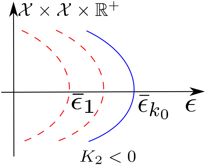
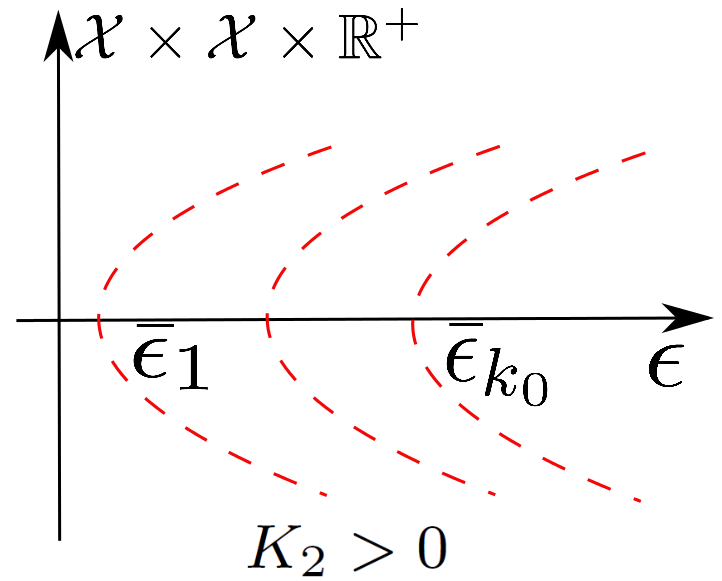
Bifurcation branch Γk(s)subscriptΓ𝑘𝑠\Gamma_{k}(s) is transcritical if K10subscript𝐾10K_{1}\neq 0 and is pitchfork if K1=0subscript𝐾10K_{1}=0 and K20subscript𝐾20K_{2}\neq 0. Indeed, as we shall see in the coming theorem, if K10subscript𝐾10K_{1}\neq 0 the sign of K1subscript𝐾1K_{1} determines the stability of (Ak(s,x),ρk(s,x))subscript𝐴𝑘𝑠𝑥subscript𝜌𝑘𝑠𝑥(A_{k}(s,x),\rho_{k}(s,x)), and if K1=0subscript𝐾10K_{1}=0 we need to determine the sign of K2subscript𝐾2K_{2}. Now we present the stability of the bifurcating solution (Ak(s,x),ρk(s,x))subscript𝐴𝑘𝑠𝑥subscript𝜌𝑘𝑠𝑥(A_{k}(s,x),\rho_{k}(s,x)) in the following theorem.

Theorem 5.1.

Suppose that all conditions in Theorem 4.1 hold. Assume that ϵ¯k0=maxkN+ϵ¯ksubscript¯italic-ϵsubscript𝑘0subscript𝑘superscript𝑁subscript¯italic-ϵ𝑘\bar{\epsilon}_{k_{0}}=\max_{k\in{N}^{+}}\bar{\epsilon}_{k}. Then for all kk0𝑘subscript𝑘0k\neq k_{0}, the steady state (Ak(s,x),ρk(s,x))subscript𝐴𝑘𝑠𝑥subscript𝜌𝑘𝑠𝑥(A_{k}(s,x),\rho_{k}(s,x)) is always unstable for s(δ,δ)𝑠𝛿𝛿s\in(-\delta,\delta). If K1<0subscript𝐾10K_{1}<0, (Ak0(s,x),ρk0(s,x))subscript𝐴subscript𝑘0𝑠𝑥subscript𝜌subscript𝑘0𝑠𝑥(A_{k_{0}}(s,x),\rho_{k_{0}}(s,x)) is asymptotically stable for s(0,δ)𝑠0𝛿s\in(0,\delta) and is unstable for s(δ,0)𝑠𝛿0s\in(-\delta,0); if K1>0subscript𝐾10K_{1}>0, (Ak0(s,x),ρk0(s,x))subscript𝐴subscript𝑘0𝑠𝑥subscript𝜌subscript𝑘0𝑠𝑥(A_{k_{0}}(s,x),\rho_{k_{0}}(s,x)) is asymptotically stable for s(δ,0)𝑠𝛿0s\in(-\delta,0) and is unstable for s(0,δ)𝑠0𝛿s\in(0,\delta); moreover, if K1=0subscript𝐾10K_{1}=0, then (Ak0(s,x),ρk0(s,x))subscript𝐴subscript𝑘0𝑠𝑥subscript𝜌subscript𝑘0𝑠𝑥(A_{k_{0}}(s,x),\rho_{k_{0}}(s,x)) is asymptotically stable for s(δ,δ)𝑠𝛿𝛿s\in(-\delta,\delta) if K2<0subscript𝐾20K_{2}<0 and is unstable if K2>0subscript𝐾20K_{2}>0.

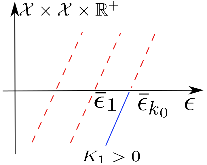
Transcritical and pitchfork bifurcations are schematically presented in Figure 1 to illustrate the stability results in Theorem 5.1.
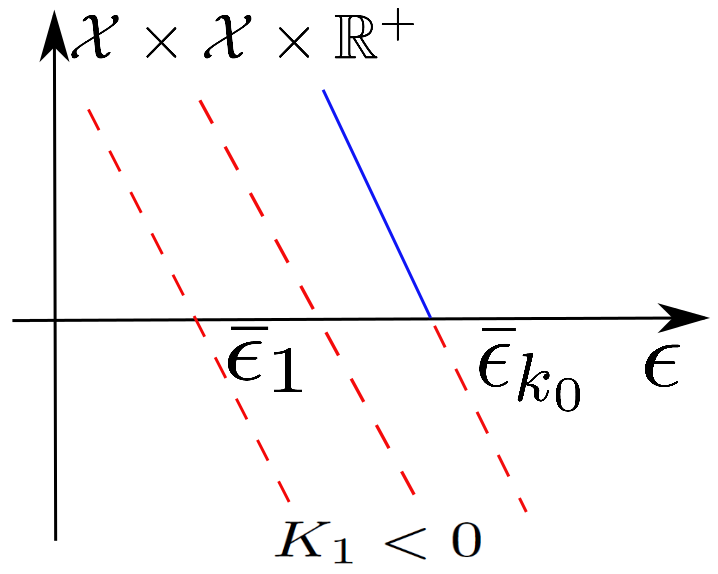
Refer to caption
Sub-transcritical
Refer to caption
Super-transcritical
Refer to caption
Sub-pitchfork
Refer to caption
Super-pitchfork
Figure 1: Transcritical and pitchfork bifurcations to system (4.1). Stable bifurcation branches are presented in solid lines and unstable branches are in dashed lines. The only stable branch must be the portion of the rightmost one that turns to the left.
Proof.

To study the stability of (Ak(s,x),ρk(s,x))subscript𝐴𝑘𝑠𝑥subscript𝜌𝑘𝑠𝑥(A_{k}(s,x),\rho_{k}(s,x)), we linearize (1.2) around this steady state and obtain the eigenvalue problem

D(A,ρ)(Ak(s,x),ρk(s,x),ϵ¯k(s))(A,ρ)=μk(s)(A,ρ),(A,ρ)𝒳×𝒳.formulae-sequencesubscript𝐷𝐴𝜌subscript𝐴𝑘𝑠𝑥subscript𝜌𝑘𝑠𝑥subscript¯italic-ϵ𝑘𝑠𝐴𝜌subscript𝜇𝑘𝑠𝐴𝜌𝐴𝜌𝒳𝒳D_{(A,\rho)}\mathcal{F}(A_{k}(s,x),\rho_{k}(s,x),\bar{\epsilon}_{k}(s))(A,\rho)=\mu_{k}(s)(A,\rho),~{}(A,\rho)\in\mathcal{X}\times\mathcal{X}. (5.6)

We first show that (Ak(s,x),ρk(s,x))subscript𝐴𝑘𝑠𝑥subscript𝜌𝑘𝑠𝑥(A_{k}(s,x),\rho_{k}(s,x)), s(δ,δ)𝑠𝛿𝛿s\in(-\delta,\delta) is always unstable for all kk0𝑘subscript𝑘0k\neq k_{0} and to this end we shall only need to show that eigenvalue μk(s)subscript𝜇𝑘𝑠\mu_{k}(s) has positive real part. According to Corollary 1.13 in [13], μk=μk(s)subscript𝜇𝑘subscript𝜇𝑘𝑠\mu_{k}=\mu_{k}(s) is a smooth function of s:(δ,δ)R:𝑠𝛿𝛿𝑅s:(-\delta,\delta)\rightarrow{R}. Sending s0𝑠0s\rightarrow 0, we see that (5.6) becomes

{ϵ¯k(η(A¯)+η(A¯)B¯)ΔA+(ρ¯1)A+A¯ρ=μk(0)A,xΩ,Δρ2ρ¯f(A¯)f(A¯)ΔAλ0ρ¯Aλ0A¯ρ=μk(0)ρ,xΩ,A𝐧=ρ𝐧=0,xΩ.casessubscript¯italic-ϵ𝑘𝜂¯𝐴superscript𝜂¯𝐴¯𝐵Δ𝐴¯𝜌1𝐴¯𝐴𝜌subscript𝜇𝑘0𝐴𝑥ΩΔ𝜌2¯𝜌superscript𝑓¯𝐴𝑓¯𝐴Δ𝐴subscript𝜆0¯𝜌𝐴subscript𝜆0¯𝐴𝜌subscript𝜇𝑘0𝜌𝑥Ω𝐴𝐧𝜌𝐧0𝑥Ω\left\{\begin{array}[]{ll}\bar{\epsilon}_{k}(\eta(\bar{A})+\eta^{\prime}(\bar{A})\bar{B})\Delta A+(\bar{\rho}-1)A+\bar{A}\rho=\mu_{k}(0)A,&x\in\Omega,\\ \Delta\rho-\frac{2\bar{\rho}f^{\prime}(\bar{A})}{f(\bar{A})}\Delta A-\lambda_{0}\bar{\rho}A-\lambda_{0}\bar{A}\rho=\mu_{k}(0)\rho,&x\in\Omega,\\ \frac{\partial A}{\partial\mathbf{n}}=\frac{\partial\rho}{\partial\mathbf{n}}=0,&x\in\partial\Omega.\end{array}\right. (5.7)

Multiplying (5.7) by ΦksubscriptΦ𝑘\Phi_{k} and integrating it over ΩΩ\Omega by parts, we have that

(ϵ¯k(η(A¯)+η(A¯)B¯)σk+ρ¯1μk(0)A¯2ρ¯f(A¯)f(A¯)σkλ0ρ¯σkλ0A¯μk(0))(ΩAΦk𝑑xΩρΦk𝑑x)=(00),\left(\begin{array}[]{cc}-\bar{\epsilon}_{k}(\eta(\bar{A})+\eta\prime(\bar{A})\bar{B})\sigma_{k}+\bar{\rho}-1-\mu_{k}(0)&\bar{A}\\ \frac{2\bar{\rho}f^{\prime}(\bar{A})}{f(\bar{A})}\sigma_{k}-\lambda_{0}\bar{\rho}&-\sigma_{k}-\lambda_{0}\bar{A}-\mu_{k}(0)\\ \end{array}\right)\left(\begin{array}[]{cc}\int_{\Omega}A\Phi_{k}dx\\ \int_{\Omega}\rho\Phi_{k}dx\end{array}\right)=\left(\begin{array}[]{cc}0\\ 0\end{array}\right),

therefore μk(0)subscript𝜇𝑘0\mu_{k}(0) is an eigenvalue of the characteristic polynomial gk(μ)=μ2+Trkμ+Detksubscript𝑔𝑘𝜇superscript𝜇2subscriptTr𝑘𝜇subscriptDet𝑘g_{k}(\mu)=\mu^{2}+\text{Tr}_{k}\mu+\text{Det}_{k}, where

Trk=ϵ¯k(η(A¯)+η(A¯)B¯)σk+1ρ¯+σk+λ0A¯\text{Tr}_{k}=\bar{\epsilon}_{k}\left(\eta(\bar{A})+\eta\prime(\bar{A})\bar{B}\right)\sigma_{k}+1-\bar{\rho}+\sigma_{k}+\lambda_{0}\bar{A}

and

Detk=(ϵ¯k(η(A¯)+η(A¯)B¯)σk+1ρ¯)(σk+λ0A¯)A¯(2ρ¯f(A¯)f(A¯)σkλ0ρ¯).\text{Det}_{k}=\left(\bar{\epsilon}_{k}\left(\eta(\bar{A})+\eta\prime(\bar{A})\bar{B}\right)\sigma_{k}+1-\bar{\rho}\right)\left(\sigma_{k}+\lambda_{0}\bar{A}\right)-\bar{A}\big{(}\frac{2\bar{\rho}f^{\prime}(\bar{A})}{f(\bar{A})}\sigma_{k}-\lambda_{0}\bar{\rho}\big{)}.

Trk>0subscriptTr𝑘0\text{Tr}_{k}>0 since ρ¯=B¯A0+B¯<1¯𝜌¯𝐵superscript𝐴0¯𝐵1\bar{\rho}=\frac{\bar{B}}{A^{0}+\bar{B}}<1 and Detk<0subscriptDet𝑘0\text{Det}_{k}<0 since ϵ¯k<ϵ¯k0=maxkN+ϵ¯ksubscript¯italic-ϵ𝑘subscript¯italic-ϵsubscript𝑘0subscript𝑘superscript𝑁subscript¯italic-ϵ𝑘\bar{\epsilon}_{k}<\bar{\epsilon}_{k_{0}}=\max_{k\in{N}^{+}}\bar{\epsilon}_{k}, therefore for any kk0𝑘subscript𝑘0k\neq k_{0}, the characteristic polynomial gk(μ)=0subscript𝑔𝑘𝜇0g_{k}(\mu)=0 always has one positive root hence (5.7) must have an eigenvalue μk(0)subscript𝜇𝑘0\mu_{k}(0) that has a positive real part. From the standard eigenvalue perturbation theory in [25], (5.6) always has a positive root μk(s)subscript𝜇𝑘𝑠\mu_{k}(s) for each kk0𝑘subscript𝑘0k\neq k_{0} when s𝑠s is small and this verifies the instability of (Ak(s,x),ρk(s,x))subscript𝐴𝑘𝑠𝑥subscript𝜌𝑘𝑠𝑥(A_{k}(s,x),\rho_{k}(s,x)) around (A¯,ρ¯k)¯𝐴subscript¯𝜌𝑘(\bar{A},\bar{\rho}_{k}).

To show that (Ak0(s,x),ρk0(s,x))subscript𝐴subscript𝑘0𝑠𝑥subscript𝜌subscript𝑘0𝑠𝑥(A_{k_{0}}(s,x),\rho_{k_{0}}(s,x)) on bifurcation branch Γk0(s)subscriptΓsubscript𝑘0𝑠\Gamma_{k_{0}}(s) are asymptotically stable, it suffcies to show that the real parts of all eigenvalues of D(A,ρ)(Ak0(s,x),ρk0(s,x),ϵ¯k0(s))subscript𝐷𝐴𝜌subscript𝐴subscript𝑘0𝑠𝑥subscript𝜌subscript𝑘0𝑠𝑥subscript¯italic-ϵsubscript𝑘0𝑠D_{(A,\rho)}\mathcal{F}(A_{k_{0}}(s,x),\rho_{k_{0}}(s,x),\bar{\epsilon}_{k_{0}}(s)) in (5.6) are negative. First of all, applying the same arguments that lead to the Fredholmness for Theorem 4.1, we can show that 0 is a K–simple eigenvalue of D(A,ρ)(A¯,ρ¯,ϵ¯k0)subscript𝐷𝐴𝜌¯𝐴¯𝜌subscript¯italic-ϵsubscript𝑘0D_{(A,\rho)}\mathcal{F}(\bar{A},\bar{\rho},\bar{\epsilon}_{k_{0}})–see Definition 1.2 in [13]. According to Corollary 1.13 in [13], there exists an interval I𝐼I with ϵ¯k0Isubscript¯italic-ϵsubscript𝑘0𝐼\bar{\epsilon}_{k_{0}}\in I and continuously differentiable functions ν(ϵ):IR:𝜈italic-ϵ𝐼𝑅\nu(\epsilon):I\rightarrow{R} and μk0(s):(δ,δ)R:subscript𝜇subscript𝑘0𝑠𝛿𝛿𝑅\mu_{k_{0}}(s):(-\delta,\delta)\rightarrow{R} such that ν=ν(ϵ)𝜈𝜈italic-ϵ\nu=\nu(\epsilon) is a real eigenvalue of

D(A,ρ)(A¯,ρ¯,ϵ)(A,ρ)=ν(ϵ)(A,ρ),(A,ρ)𝒳×𝒳formulae-sequencesubscript𝐷𝐴𝜌¯𝐴¯𝜌italic-ϵ𝐴𝜌𝜈italic-ϵ𝐴𝜌𝐴𝜌𝒳𝒳D_{(A,\rho)}\mathcal{F}(\bar{A},\bar{\rho},\epsilon)(A,\rho)=\nu(\epsilon)(A,\rho),(A,\rho)\in\mathcal{X}\times\mathcal{X} (5.8)

with ν(ϵ¯k0)=0𝜈subscript¯italic-ϵsubscript𝑘00\nu(\bar{\epsilon}_{k_{0}})=0 and μk0=μk0(s)subscript𝜇subscript𝑘0subscript𝜇subscript𝑘0𝑠\mu_{k_{0}}=\mu_{k_{0}}(s) is an eigenvalue of (5.6) with μk0(0)=0subscript𝜇subscript𝑘000\mu_{k_{0}}(0)=0 ; moreover ν(ϵ¯k0)𝜈subscript¯italic-ϵsubscript𝑘0\nu(\bar{\epsilon}_{k_{0}}) is the only eigenvalue of (5.8) for any fixed neighbourhood of the origin of the complex plane; furthermore, the eigenfunction of (5.8) depends on ϵitalic-ϵ\epsilon smoothly and can be written as (A(ϵ,x),ρ(ϵ,x))𝐴italic-ϵ𝑥𝜌italic-ϵ𝑥(A(\epsilon,x),\rho(\epsilon,x)), which is uniquely determined by (A(ϵ¯k0,x),ρ(ϵ¯k0,x))=(A¯k0,ρ¯k0)𝐴subscript¯italic-ϵsubscript𝑘0𝑥𝜌subscript¯italic-ϵsubscript𝑘0𝑥subscript¯𝐴subscript𝑘0subscript¯𝜌subscript𝑘0(A(\bar{\epsilon}_{k_{0}},x),\rho(\bar{\epsilon}_{k_{0}},x))=(\bar{A}_{k_{0}},\bar{\rho}_{k_{0}}) and (A(ϵ,x),ρ(ϵ,x))(A¯k0,ρ¯k0)𝒵𝐴italic-ϵ𝑥𝜌italic-ϵ𝑥subscript¯𝐴subscript𝑘0subscript¯𝜌subscript𝑘0𝒵(A(\epsilon,x),\rho(\epsilon,x))-(\bar{A}_{k_{0}},\bar{\rho}_{k_{0}})\in\mathcal{Z}.

We now proceed to evaluate the sign of μk0(s)subscript𝜇subscript𝑘0𝑠\mu_{k_{0}}(s) for s(δ,δ)𝑠𝛿𝛿s\in(-\delta,\delta). Differentiating (5.8) with respect to ϵitalic-ϵ\epsilon and putting ϵ=ϵ¯k0italic-ϵsubscript¯italic-ϵsubscript𝑘0\epsilon=\bar{\epsilon}_{k_{0}}, we have that

{ϵ¯k0(η(A¯)+η(A¯)B¯)ΔA˙+(ρ¯1)A˙+A¯ρ˙+(η(A¯)+η(A¯)B¯)ΔA¯k0=ν˙(ϵ¯k0)A¯k0,Δρ˙2ρ¯f(A¯)f(A¯)ΔA˙λ0ρ¯A˙λ0A¯ρ˙=ν˙(ϵ¯k0)ρ¯k0,casessubscript¯italic-ϵsubscript𝑘0𝜂¯𝐴superscript𝜂¯𝐴¯𝐵Δ˙𝐴¯𝜌1˙𝐴¯𝐴˙𝜌𝜂¯𝐴superscript𝜂¯𝐴¯𝐵Δsubscript¯𝐴subscript𝑘0˙𝜈subscript¯italic-ϵsubscript𝑘0subscript¯𝐴subscript𝑘0missing-subexpressionΔ˙𝜌2¯𝜌superscript𝑓¯𝐴𝑓¯𝐴Δ˙𝐴subscript𝜆0¯𝜌˙𝐴subscript𝜆0¯𝐴˙𝜌˙𝜈subscript¯italic-ϵsubscript𝑘0subscript¯𝜌subscript𝑘0missing-subexpression\left\{\begin{array}[]{ll}\bar{\epsilon}_{k_{0}}(\eta(\bar{A})+\eta^{\prime}(\bar{A})\bar{B})\Delta\dot{A}+(\bar{\rho}-1)\dot{A}+\bar{A}\dot{\rho}+(\eta(\bar{A})+\eta^{\prime}(\bar{A})\bar{B})\Delta\bar{A}_{k_{0}}=\dot{\nu}(\bar{\epsilon}_{k_{0}})\bar{A}_{k_{0}},\\ \Delta\dot{\rho}-\frac{2\bar{\rho}f^{\prime}(\bar{A})}{f(\bar{A})}\Delta\dot{A}-\lambda_{0}\bar{\rho}\dot{A}-\lambda_{0}\bar{A}\dot{\rho}=\dot{\nu}(\bar{\epsilon}_{k_{0}})\bar{\rho}_{k_{0}},\end{array}\right. (5.9)

where A˙=A(ϵ,x)ϵ|ϵ=ϵ¯k0˙𝐴evaluated-at𝐴italic-ϵ𝑥italic-ϵitalic-ϵsubscript¯italic-ϵsubscript𝑘0\dot{A}=\frac{\partial A(\epsilon,x)}{\partial\epsilon}|_{\epsilon=\bar{\epsilon}_{k_{0}}} and ρ˙=ρ(ϵ,x)ϵ|ϵ=ϵ¯k0˙𝜌evaluated-at𝜌italic-ϵ𝑥italic-ϵitalic-ϵsubscript¯italic-ϵsubscript𝑘0\dot{\rho}=\frac{\partial\rho(\epsilon,x)}{\partial\epsilon}|_{\epsilon=\bar{\epsilon}_{k_{0}}}. Testing (5.9) by Φk0subscriptΦsubscript𝑘0\Phi_{k_{0}} gives rise to

(ϵ¯k0(η(A¯)+η(A¯)B¯)σk0+ρ¯1A¯2ρ¯f(A¯)f(A¯)σk0λ0ρ¯σk0λ0A¯)(ΩA˙Φk0𝑑xΩρ˙Φk0𝑑x)=(ν˙(ϵ¯k0)Qk0+ϵ¯k0(η(A¯)+η(A¯)B¯)Qk0ν˙(ϵ¯k0),)\begin{split}&\begin{pmatrix}-\bar{\epsilon}_{k_{0}}(\eta(\bar{A})+\eta\prime(\bar{A})\bar{B})\sigma_{k_{0}}+\bar{\rho}-1&\bar{A}\\ \frac{2\bar{\rho}f^{\prime}(\bar{A})}{f(\bar{A})}\sigma_{k_{0}}-\lambda_{0}\bar{\rho}&-\sigma_{k_{0}}-\lambda_{0}\bar{A}\\ \end{pmatrix}\begin{pmatrix}\int_{\Omega}\dot{A}\Phi_{k_{0}}dx\\ \int_{\Omega}\dot{\rho}\Phi_{k_{0}}dx\end{pmatrix}\\ =&\begin{pmatrix}\dot{\nu}(\bar{\epsilon}_{k_{0}})Q_{k_{0}}+\bar{\epsilon}_{k_{0}}(\eta(\bar{A})+\eta^{\prime}(\bar{A})\bar{B})Q_{k_{0}}\\ \dot{\nu}(\bar{\epsilon}_{k_{0}}),\end{pmatrix}\end{split} (5.10)

where we have used the fact that ΩΦk02𝑑x=1subscriptΩsubscriptsuperscriptΦ2subscript𝑘0differential-d𝑥1\int_{\Omega}\Phi^{2}_{k_{0}}dx=1. The coefficient matrix in (5.10) is singular in light of (4.7), therefore

A¯σk0λ0A¯=ν˙(ϵ¯k0)Qk0+ϵ¯k0(η(A¯)+η(A¯)B¯)Qk0ν˙(ϵ¯k0)¯𝐴subscript𝜎subscript𝑘0subscript𝜆0¯𝐴˙𝜈subscript¯italic-ϵsubscript𝑘0subscript𝑄subscript𝑘0subscript¯italic-ϵsubscript𝑘0𝜂¯𝐴superscript𝜂¯𝐴¯𝐵subscript𝑄subscript𝑘0˙𝜈subscript¯italic-ϵsubscript𝑘0\frac{\bar{A}}{-\sigma_{k_{0}}-\lambda_{0}\bar{A}}=\frac{\dot{\nu}(\bar{\epsilon}_{k_{0}})Q_{k_{0}}+\bar{\epsilon}_{k_{0}}(\eta(\bar{A})+\eta^{\prime}(\bar{A})\bar{B})Q_{k_{0}}}{\dot{\nu}(\bar{\epsilon}_{k_{0}})}

and consequently we can easily show that ν˙(ϵ¯k0)<0˙𝜈subscript¯italic-ϵsubscript𝑘00\dot{\nu}(\bar{\epsilon}_{k_{0}})<0. According to (1.17) in Theorem 1.16 of [13], μk0(s)subscript𝜇subscript𝑘0𝑠\mu_{k_{0}}(s) and sϵ¯k0(s)ν˙(ϵ¯k0)𝑠subscriptsuperscript¯italic-ϵsubscript𝑘0𝑠˙𝜈subscript¯italic-ϵsubscript𝑘0-s\bar{\epsilon}^{\prime}_{k_{0}}(s)\dot{\nu}(\bar{\epsilon}_{k_{0}}) have the same zeros and the same signs near s=0𝑠0s=0, and for μk0(s)0subscript𝜇subscript𝑘0𝑠0\mu_{k_{0}}(s)\neq 0

lims0sϵ¯k0(s)ν˙(ϵ¯k0)μk0(s)=1,subscript𝑠0𝑠subscriptsuperscript¯italic-ϵsubscript𝑘0𝑠˙𝜈subscript¯italic-ϵsubscript𝑘0subscript𝜇subscript𝑘0𝑠1\lim_{s\rightarrow 0}\frac{-s\bar{\epsilon}^{\prime}_{k_{0}}(s)\dot{\nu}(\bar{\epsilon}_{k_{0}})}{\mu_{k_{0}}(s)}=1,

where the dot sign denotes the differentiation with respect to ϵitalic-ϵ\epsilon. Therefore, we have that sgn(μk0(s))=sgn(K1)sgnsubscript𝜇subscript𝑘0𝑠sgnsubscript𝐾1\text{sgn}(\mu_{k_{0}}(s))=\text{sgn}(K_{1}) if K10subscript𝐾10K_{1}\neq 0 and sgn(μk0(s))=sgn(K2)sgnsubscript𝜇subscript𝑘0𝑠sgnsubscript𝐾2\text{sgn}(\mu_{k_{0}}(s))=\text{sgn}(K_{2}) if K1=0subscript𝐾10K_{1}=0 and K20subscript𝐾20K_{2}\neq 0. On the other hand, we already see from the analysis above that the other eigen-value of (5.6) for k=k0𝑘subscript𝑘0k=k_{0} is negative, therefore Theorem 5.1 readily follows from the arguments above. \mathchar 1027\relax

Remark 5.1.

Theorem 5.1 indicates that, only the k0subscript𝑘0k_{0}–th bifurcation branch Γk0(s)subscriptΓsubscript𝑘0𝑠\Gamma_{k_{0}}(s) around (A¯,ρ¯)¯𝐴¯𝜌(\bar{A},\bar{\rho}) can be stable. In other words, if a spatial pattern is stable, it must be on the branch Γk0(s)subscriptΓsubscript𝑘0𝑠\Gamma_{k_{0}}(s) for which ϵ¯ksubscript¯italic-ϵ𝑘\bar{\epsilon}_{k} is maximized over N+superscript𝑁{N}^{+}. This selection of principal wavemode provides essential understandings of pattern formations in model (1.2), i.e., stable patterns must develop in terms of the principal mode Φk0subscriptΦsubscript𝑘0\Phi_{k_{0}} if ϵitalic-ϵ\epsilon is taken to be smaller than but close to ϵ¯k0subscript¯italic-ϵsubscript𝑘0\bar{\epsilon}_{k_{0}}. An important implication of this wavemode selection mechanism is that larger domain tends to support stable patterns with more modes. To elucidate this result, we consider the one–dimensional domain Ω=(0,L)Ω0𝐿\Omega=(0,L) which has σk=(kπL)2subscript𝜎𝑘superscript𝑘𝜋𝐿2\sigma_{k}=\big{(}\frac{k\pi}{L}\big{)}^{2} as its Neumann eigenvalue. Denote ϵ¯k1=maxkN+ϵ¯ksubscript¯italic-ϵsubscript𝑘1subscript𝑘superscript𝑁subscript¯italic-ϵ𝑘\bar{\epsilon}_{k_{1}}=\max_{k\in{N}^{+}}\bar{\epsilon}_{k} for L=L1𝐿subscript𝐿1L=L_{1} and ϵ¯k2=maxkN+ϵ¯ksubscript¯italic-ϵsubscript𝑘2subscript𝑘superscript𝑁subscript¯italic-ϵ𝑘\bar{\epsilon}_{k_{2}}=\max_{k\in{N}^{+}}\bar{\epsilon}_{k} for L=L2𝐿subscript𝐿2L=L_{2}, then we must have that k1<k2subscript𝑘1subscript𝑘2k_{1}<k_{2} if L1<L2subscript𝐿1subscript𝐿2L_{1}<L_{2}. Similar results hold in multi-dimensional domains (under Dirichlet Boundary conditions). Figure 3 in Section 6 verifies this observation numerically. Such wavemode selection mechanism was found for a volume filling chemotaxis model with logistic growth in [28].

5.1 Bifurcation of transcritical type

We proceed to find the values of K1subscript𝐾1K_{1} and K2subscript𝐾2K_{2} given in (5.1). To this end, we first give the following Taylor expansions from straightforward calculations

η(A)=η(A¯)+sη(A¯)QkΦk+s2(η(A¯)ψ1+12η′′(A¯)Qk2Φk2)+s3(η(A¯)ψ2+η′′(A¯)Qkψ1Φk+η′′′(A¯)6Qk3Φk3)+o(s3).𝜂𝐴𝜂¯𝐴𝑠superscript𝜂¯𝐴subscript𝑄𝑘subscriptΦ𝑘superscript𝑠2superscript𝜂¯𝐴subscript𝜓112superscript𝜂′′¯𝐴superscriptsubscript𝑄𝑘2superscriptsubscriptΦ𝑘2superscript𝑠3superscript𝜂¯𝐴subscript𝜓2superscript𝜂′′¯𝐴subscript𝑄𝑘subscript𝜓1subscriptΦ𝑘superscript𝜂′′′¯𝐴6superscriptsubscript𝑄𝑘3superscriptsubscriptΦ𝑘3𝑜superscript𝑠3\begin{split}\eta(A)=&\eta(\bar{A})+s\eta^{\prime}(\bar{A})Q_{k}\Phi_{k}+s^{2}\Big{(}\eta^{\prime}(\bar{A})\psi_{1}+\frac{1}{2}\eta^{\prime\prime}(\bar{A})Q_{k}^{2}\Phi_{k}^{2}\Big{)}+s^{3}\Big{(}\eta^{\prime}(\bar{A})\psi_{2}\\ &+\eta^{\prime\prime}(\bar{A})Q_{k}\psi_{1}\Phi_{k}+\frac{\eta^{\prime\prime\prime}(\bar{A})}{6}Q_{k}^{3}\Phi_{k}^{3}\Big{)}+o(s^{3}).\end{split} (5.11)

Substituting (5.1) and (5.11) into (4.1), we collect the s2superscript𝑠2s^{2}–terms there to obtain

K1(η(A¯)+η(A¯)B¯)QkσkΦk=(η(A¯)+η(A¯)B¯)ϵ¯kΔψ1+(ρ¯1)ψ1+A¯φ1+(2η(A¯)+η′′(A¯)B¯)Qk2ϵ¯k|Φk|2+(Qk(2η(A¯)+η′′(A¯)B¯)Qk2ϵ¯kσk)Φk2.subscript𝐾1𝜂¯𝐴superscript𝜂¯𝐴¯𝐵subscript𝑄𝑘subscript𝜎𝑘subscriptΦ𝑘𝜂¯𝐴superscript𝜂¯𝐴¯𝐵subscript¯italic-ϵ𝑘Δsubscript𝜓1¯𝜌1subscript𝜓1¯𝐴subscript𝜑12superscript𝜂¯𝐴superscript𝜂′′¯𝐴¯𝐵superscriptsubscript𝑄𝑘2subscript¯italic-ϵ𝑘superscriptsubscriptΦ𝑘2subscript𝑄𝑘2superscript𝜂¯𝐴superscript𝜂′′¯𝐴¯𝐵superscriptsubscript𝑄𝑘2subscript¯italic-ϵ𝑘subscript𝜎𝑘superscriptsubscriptΦ𝑘2\begin{split}K_{1}(\eta(\bar{A})+\eta^{\prime}(\bar{A})\bar{B})Q_{k}\sigma_{k}\Phi_{k}=&(\eta(\bar{A})+\eta^{\prime}(\bar{A})\bar{B})\bar{\epsilon}_{k}\Delta\psi_{1}+(\bar{\rho}-1)\psi_{1}+\bar{A}\varphi_{1}\\ &+(2\eta^{\prime}(\bar{A})+\eta^{\prime\prime}(\bar{A})\bar{B})Q_{k}^{2}\bar{\epsilon}_{k}|\nabla\Phi_{k}|^{2}\\ &+(Q_{k}-(2\eta^{\prime}(\bar{A})+\eta^{\prime\prime}(\bar{A})\bar{B})Q_{k}^{2}\bar{\epsilon}_{k}\sigma_{k})\Phi_{k}^{2}.\end{split} (5.12)
Proof.

of Proposition 5.1. Multiplying (5.12) by ΦksubscriptΦ𝑘\Phi_{k} and then integrating it over ΩΩ\Omega by parts, we obtain that

K1(η(A¯)+η(A¯)B¯)Qkσk=(ρ¯1(η(A¯)+η(A¯)B¯)ϵ¯kσk)Ωψ1Φk𝑑x+A¯Ωφ1Φk𝑑x+(2η(A¯)+η′′(A¯)B¯)Qk2ϵ¯kΩΦk|Φk|2𝑑x+(Qk(2η(A¯)+η′′(A¯)B¯)Qk2ϵ¯kσk)ΩΦk3𝑑x=(ρ¯1(η(A¯)+η(A¯)B¯)ϵ¯kσk)Ωψ1Φk𝑑x+A¯Ωφ1Φk𝑑x+(Qk(η(A¯)+12η′′(A¯)B¯)Qk2ϵ¯kσk)ΩΦk3𝑑x,subscript𝐾1𝜂¯𝐴superscript𝜂¯𝐴¯𝐵subscript𝑄𝑘subscript𝜎𝑘¯𝜌1𝜂¯𝐴superscript𝜂¯𝐴¯𝐵subscript¯italic-ϵ𝑘subscript𝜎𝑘subscriptΩsubscript𝜓1subscriptΦ𝑘differential-d𝑥¯𝐴subscriptΩsubscript𝜑1subscriptΦ𝑘differential-d𝑥2superscript𝜂¯𝐴superscript𝜂′′¯𝐴¯𝐵superscriptsubscript𝑄𝑘2subscript¯italic-ϵ𝑘subscriptΩsubscriptΦ𝑘superscriptsubscriptΦ𝑘2differential-d𝑥subscript𝑄𝑘2superscript𝜂¯𝐴superscript𝜂′′¯𝐴¯𝐵superscriptsubscript𝑄𝑘2subscript¯italic-ϵ𝑘subscript𝜎𝑘subscriptΩsuperscriptsubscriptΦ𝑘3differential-d𝑥¯𝜌1𝜂¯𝐴superscript𝜂¯𝐴¯𝐵subscript¯italic-ϵ𝑘subscript𝜎𝑘subscriptΩsubscript𝜓1subscriptΦ𝑘differential-d𝑥¯𝐴subscriptΩsubscript𝜑1subscriptΦ𝑘differential-d𝑥subscript𝑄𝑘superscript𝜂¯𝐴12superscript𝜂′′¯𝐴¯𝐵superscriptsubscript𝑄𝑘2subscript¯italic-ϵ𝑘subscript𝜎𝑘subscriptΩsuperscriptsubscriptΦ𝑘3differential-d𝑥\begin{split}&K_{1}(\eta(\bar{A})+\eta^{\prime}(\bar{A})\bar{B})Q_{k}\sigma_{k}\\ =&\Big{(}\bar{\rho}-1-(\eta(\bar{A})+\eta^{\prime}(\bar{A})\bar{B})\bar{\epsilon}_{k}\sigma_{k}\Big{)}\int_{\Omega}\psi_{1}\Phi_{k}dx+\bar{A}\int_{\Omega}\varphi_{1}\Phi_{k}dx\\ &+(2\eta^{\prime}(\bar{A})+\eta^{\prime\prime}(\bar{A})\bar{B})Q_{k}^{2}\bar{\epsilon}_{k}\int_{\Omega}\Phi_{k}|\nabla\Phi_{k}|^{2}dx\\ &+(Q_{k}-(2\eta^{\prime}(\bar{A})+\eta^{\prime\prime}(\bar{A})\bar{B})Q_{k}^{2}\bar{\epsilon}_{k}\sigma_{k})\int_{\Omega}\Phi_{k}^{3}dx\\ =&\big{(}\bar{\rho}-1-(\eta(\bar{A})+\eta^{\prime}(\bar{A})\bar{B})\bar{\epsilon}_{k}\sigma_{k}\big{)}\int_{\Omega}\psi_{1}\Phi_{k}dx+\bar{A}\int_{\Omega}\varphi_{1}\Phi_{k}dx\\ &+\big{(}Q_{k}-(\eta^{\prime}(\bar{A})+\frac{1}{2}\eta^{\prime\prime}(\bar{A})\bar{B})Q_{k}^{2}\bar{\epsilon}_{k}\sigma_{k}\big{)}\int_{\Omega}\Phi_{k}^{3}dx,\end{split} (5.13)

where we have applied the fact Ω|Φk|2Φk𝑑x=σk2ΩΦk3𝑑xsubscriptΩsuperscriptsubscriptΦ𝑘2subscriptΦ𝑘differential-d𝑥subscript𝜎𝑘2subscriptΩsuperscriptsubscriptΦ𝑘3differential-d𝑥\int_{\Omega}|\nabla\Phi_{k}|^{2}\Phi_{k}dx=\frac{\sigma_{k}}{2}\int_{\Omega}\Phi_{k}^{3}dx because

ΩΦk|Φk|2𝑑x=12ΩΦk2Φkdx=12Ω((Φk2Φk)Φk2ΔΦk)𝑑x=12ΩΦk2ΔΦk𝑑x=σk2ΩΦk3𝑑x.subscriptΩsubscriptΦ𝑘superscriptsubscriptΦ𝑘2differential-d𝑥12subscriptΩsuperscriptsubscriptΦ𝑘2subscriptΦ𝑘𝑑𝑥12subscriptΩsuperscriptsubscriptΦ𝑘2subscriptΦ𝑘superscriptsubscriptΦ𝑘2ΔsubscriptΦ𝑘differential-d𝑥12subscriptΩsuperscriptsubscriptΦ𝑘2ΔsubscriptΦ𝑘differential-d𝑥subscript𝜎𝑘2subscriptΩsuperscriptsubscriptΦ𝑘3differential-d𝑥\begin{split}\int_{\Omega}\Phi_{k}|\nabla\Phi_{k}|^{2}dx&=\frac{1}{2}\int_{\Omega}\nabla\Phi_{k}^{2}\cdot\nabla\Phi_{k}dx=\frac{1}{2}\int_{\Omega}(\nabla\cdot(\Phi_{k}^{2}\nabla\Phi_{k})-\Phi_{k}^{2}\Delta\Phi_{k})dx\\ &=-\frac{1}{2}\int_{\Omega}\Phi_{k}^{2}\Delta\Phi_{k}dx=\frac{\sigma_{k}}{2}\int_{\Omega}\Phi_{k}^{3}dx.\end{split}

Substituting (5.1) into the ρ𝜌\rho–equation of (4.1), we collect the s2superscript𝑠2s^{2}–terms to have

Δφ12ρ¯f(A¯)f(A¯)Δψ1λ0ρ¯ψ1λ0A¯φ1(2f(A¯)f(A¯)+2ρ¯(f′′(A¯)f(A¯)f(A¯)2f(A¯)2)Qk)Qk|Φk|2+((2f(A¯)f(A¯)+2ρ¯(f′′(A¯)f(A¯)f(A¯)2f(A¯)2)Qk)Qkσkλ0Qk)Φk2=0.Δsubscript𝜑12¯𝜌superscript𝑓¯𝐴𝑓¯𝐴Δsubscript𝜓1subscript𝜆0¯𝜌subscript𝜓1subscript𝜆0¯𝐴subscript𝜑12superscript𝑓¯𝐴𝑓¯𝐴2¯𝜌superscript𝑓′′¯𝐴𝑓¯𝐴superscript𝑓superscript¯𝐴2𝑓superscript¯𝐴2subscript𝑄𝑘subscript𝑄𝑘superscriptsubscriptΦ𝑘22superscript𝑓¯𝐴𝑓¯𝐴2¯𝜌superscript𝑓′′¯𝐴𝑓¯𝐴superscript𝑓superscript¯𝐴2𝑓superscript¯𝐴2subscript𝑄𝑘subscript𝑄𝑘subscript𝜎𝑘subscript𝜆0subscript𝑄𝑘superscriptsubscriptΦ𝑘20\begin{split}\Delta\varphi_{1}&-\frac{2\bar{\rho}f^{\prime}(\bar{A})}{f(\bar{A})}\Delta\psi_{1}-\lambda_{0}\bar{\rho}\psi_{1}-\lambda_{0}\bar{A}\varphi_{1}-\Big{(}\frac{2f^{\prime}(\bar{A})}{f(\bar{A})}+2\bar{\rho}\Big{(}\frac{f^{\prime\prime}(\bar{A})}{f(\bar{A})}-\frac{f^{\prime}(\bar{A})^{2}}{f(\bar{A})^{2}}\Big{)}Q_{k}\Big{)}Q_{k}|\nabla\Phi_{k}|^{2}\\ &+\Big{(}\big{(}\frac{2f^{\prime}(\bar{A})}{f(\bar{A})}+2\bar{\rho}\Big{(}\frac{f^{\prime\prime}(\bar{A})}{f(\bar{A})}-\frac{f^{\prime}(\bar{A})^{2}}{f(\bar{A})^{2}}\Big{)}Q_{k}\big{)}Q_{k}\sigma_{k}-\lambda_{0}Q_{k}\Big{)}\Phi_{k}^{2}=0.\end{split} (5.14)

We test this equation by ΦksubscriptΦ𝑘\Phi_{k} over ΩΩ\Omega and obtain

(2ρ¯f(A¯)f(A¯)σkλ0ρ¯)Ωψ1Φk𝑑x(σk+λ0A¯)Ωφ1Φk𝑑x=(λ0Qk(f(A¯)f(A¯)+ρ¯(f′′(A¯)f(A¯)f(A¯)2f(A¯)2)Qk)Qkσk)ΩΦk3𝑑x;2¯𝜌superscript𝑓¯𝐴𝑓¯𝐴subscript𝜎𝑘subscript𝜆0¯𝜌subscriptΩsubscript𝜓1subscriptΦ𝑘differential-d𝑥subscript𝜎𝑘subscript𝜆0¯𝐴subscriptΩsubscript𝜑1subscriptΦ𝑘differential-d𝑥subscript𝜆0subscript𝑄𝑘superscript𝑓¯𝐴𝑓¯𝐴¯𝜌superscript𝑓′′¯𝐴𝑓¯𝐴superscript𝑓superscript¯𝐴2𝑓superscript¯𝐴2subscript𝑄𝑘subscript𝑄𝑘subscript𝜎𝑘subscriptΩsuperscriptsubscriptΦ𝑘3differential-d𝑥\begin{split}&\Big{(}\frac{2\bar{\rho}f^{\prime}(\bar{A})}{f(\bar{A})}\sigma_{k}-\lambda_{0}\bar{\rho}\Big{)}\int_{\Omega}\psi_{1}\Phi_{k}dx-(\sigma_{k}+\lambda_{0}\bar{A})\int_{\Omega}\varphi_{1}\Phi_{k}dx\\ =&\left(\lambda_{0}Q_{k}-\Big{(}\frac{f^{\prime}(\bar{A})}{f(\bar{A})}+\bar{\rho}(\frac{f^{\prime\prime}(\bar{A})}{f(\bar{A})}-\frac{f^{\prime}(\bar{A})^{2}}{f(\bar{A})^{2}})Q_{k}\Big{)}Q_{k}\sigma_{k}\right)\int_{\Omega}\Phi_{k}^{3}dx;\end{split} (5.15)

on the other hand, (ψ1,φ1)𝒵subscript𝜓1subscript𝜑1𝒵(\psi_{1},\varphi_{1})\in\mathcal{Z} in (4.12) implies that

Ω(Qkψ1+φ1)Φk𝑑x=QkΩψ1Φk𝑑x+Ωφ1Φk𝑑x=0subscriptΩsubscript𝑄𝑘subscript𝜓1subscript𝜑1subscriptΦ𝑘differential-d𝑥subscript𝑄𝑘subscriptΩsubscript𝜓1subscriptΦ𝑘differential-d𝑥subscriptΩsubscript𝜑1subscriptΦ𝑘differential-d𝑥0\int_{\Omega}(Q_{k}\psi_{1}+\varphi_{1})\Phi_{k}dx=Q_{k}\int_{\Omega}\psi_{1}\Phi_{k}dx+\int_{\Omega}\varphi_{1}\Phi_{k}dx=0 (5.16)

and solving (5.15) and (5.16) gives us

Ωψ1Φk𝑑x=(λ0Qk(f(A¯)f(A¯)+ρ¯(f′′(A¯)f(A¯)f(A¯)2f(A¯)2)Qk)Qkσk)ΩΦk3𝑑x2ρ¯f(A¯)f(A¯)σkλ0ρ¯+(σk+λ0A¯)Qk,subscriptΩsubscript𝜓1subscriptΦ𝑘differential-d𝑥subscript𝜆0subscript𝑄𝑘superscript𝑓¯𝐴𝑓¯𝐴¯𝜌superscript𝑓′′¯𝐴𝑓¯𝐴superscript𝑓superscript¯𝐴2𝑓superscript¯𝐴2subscript𝑄𝑘subscript𝑄𝑘subscript𝜎𝑘subscriptΩsuperscriptsubscriptΦ𝑘3differential-d𝑥2¯𝜌superscript𝑓¯𝐴𝑓¯𝐴subscript𝜎𝑘subscript𝜆0¯𝜌subscript𝜎𝑘subscript𝜆0¯𝐴subscript𝑄𝑘\int_{\Omega}\psi_{1}\Phi_{k}dx=\frac{\left(\lambda_{0}Q_{k}-(\frac{f^{\prime}(\bar{A})}{f(\bar{A})}+\bar{\rho}(\frac{f^{\prime\prime}(\bar{A})}{f(\bar{A})}-\frac{f^{\prime}(\bar{A})^{2}}{f(\bar{A})^{2}})Q_{k})Q_{k}\sigma_{k}\right)\int_{\Omega}\Phi_{k}^{3}dx}{\frac{2\bar{\rho}f^{\prime}(\bar{A})}{f(\bar{A})}\sigma_{k}-\lambda_{0}\bar{\rho}+(\sigma_{k}+\lambda_{0}\bar{A})Q_{k}}, (5.17)

and

Ωφ1Φk𝑑x=QkΩψ1Φk𝑑x.subscriptΩsubscript𝜑1subscriptΦ𝑘differential-d𝑥subscript𝑄𝑘subscriptΩsubscript𝜓1subscriptΦ𝑘differential-d𝑥\int_{\Omega}\varphi_{1}\Phi_{k}dx=-Q_{k}\int_{\Omega}\psi_{1}\Phi_{k}dx. (5.18)

Substituting (5.17) and (5.18) into (5.13), we can easily show (5.2) and this concludes the proof of Proposition 5.1. \mathchar 1027\relax

We see that K1subscript𝐾1K_{1} is determined by the value of ΩΦk3𝑑xsubscriptΩsuperscriptsubscriptΦ𝑘3differential-d𝑥\int_{\Omega}\Phi_{k}^{3}dx and system parameters. By the same calculations, we can also verify K1subscript𝐾1K_{1} given in (5.4) holds for (4.2).

5.2 Bifurcation of pitchfork type

If ΩΩ\Omega has a geometry such that ΩΦk3𝑑x=0subscriptΩsuperscriptsubscriptΦ𝑘3differential-d𝑥0\int_{\Omega}\Phi_{k}^{3}dx=0, for example a finite interval or multi–dimensional rectangle, ΦksubscriptΦ𝑘\Phi_{k} is a cosine function or a product of cosine functions, which implies that K1=0subscript𝐾10K_{1}=0, therefore we need to find K2subscript𝐾2K_{2} given in (5.3) to determine the stability of the bifurcating solutions.

Proof.

of Proposition 5.2. We equate the s3superscript𝑠3s^{3}–terms in (4.1) to obtain that

K2(η(A¯)+η(A¯)B¯)QkσkΦk=(2η(A¯)+η′′(A¯)B¯)Qkϵ¯k(Δψ1Φk+2ψ1Φkσkψ1Φk)+(η(A¯)+η(A¯)B¯)ϵ¯kΔψ2+(ρ¯1)ψ2+ψ1Φk+A¯φ2+Qkφ1Φk+(η′′(A¯)2+η′′′(A¯)6B¯)Qk3ϵ¯k(6Φk|Φk|23σkΦk3).subscript𝐾2𝜂¯𝐴superscript𝜂¯𝐴¯𝐵subscript𝑄𝑘subscript𝜎𝑘subscriptΦ𝑘2superscript𝜂¯𝐴superscript𝜂′′¯𝐴¯𝐵subscript𝑄𝑘subscript¯italic-ϵ𝑘Δsubscript𝜓1subscriptΦ𝑘2subscript𝜓1subscriptΦ𝑘subscript𝜎𝑘subscript𝜓1subscriptΦ𝑘𝜂¯𝐴superscript𝜂¯𝐴¯𝐵subscript¯italic-ϵ𝑘Δsubscript𝜓2¯𝜌1subscript𝜓2subscript𝜓1subscriptΦ𝑘¯𝐴subscript𝜑2subscript𝑄𝑘subscript𝜑1subscriptΦ𝑘superscript𝜂′′¯𝐴2superscript𝜂′′′¯𝐴6¯𝐵superscriptsubscript𝑄𝑘3subscript¯italic-ϵ𝑘6subscriptΦ𝑘superscriptsubscriptΦ𝑘23subscript𝜎𝑘superscriptsubscriptΦ𝑘3\begin{split}&K_{2}(\eta(\bar{A})+\eta^{\prime}(\bar{A})\bar{B})Q_{k}\sigma_{k}\Phi_{k}\\ =&(2\eta^{\prime}(\bar{A})+\eta^{\prime\prime}(\bar{A})\bar{B})Q_{k}\bar{\epsilon}_{k}(\Delta\psi_{1}\Phi_{k}+2\nabla\psi_{1}\cdot\nabla\Phi_{k}-\sigma_{k}\psi_{1}\Phi_{k})\\ &+(\eta(\bar{A})+\eta^{\prime}(\bar{A})\bar{B})\bar{\epsilon}_{k}\Delta\psi_{2}+(\bar{\rho}-1)\psi_{2}+\psi_{1}\Phi_{k}+\bar{A}\varphi_{2}\\ &+Q_{k}\varphi_{1}\Phi_{k}+\Big{(}\frac{\eta^{\prime\prime}(\bar{A})}{2}+\frac{\eta^{\prime\prime\prime}(\bar{A})}{6}\bar{B}\Big{)}Q_{k}^{3}\bar{\epsilon}_{k}(6\Phi_{k}|\nabla\Phi_{k}|^{2}-3\sigma_{k}\Phi_{k}^{3}).\end{split} (5.19)

Multiply both hand sides of (5.19) by ΦksubscriptΦ𝑘\Phi_{k} and integrate it over ΩΩ\Omega by parts, then in light of the identity ΩΦk2|Φk|2𝑑x=σk3ΩΦk4𝑑xsubscriptΩsuperscriptsubscriptΦ𝑘2superscriptsubscriptΦ𝑘2differential-d𝑥subscript𝜎𝑘3subscriptΩsuperscriptsubscriptΦ𝑘4differential-d𝑥\int_{\Omega}\Phi_{k}^{2}|\nabla\Phi_{k}|^{2}dx=\frac{\sigma_{k}}{3}\int_{\Omega}\Phi_{k}^{4}dx, we can prove (5.3) in Proposition 5.2. \mathchar 1027\relax

K2subscript𝐾2K_{2} in (5.3) is determined by the integrals Ωψ2Φk,Ωφ2Φk,Ωψ1Φk2subscriptΩsubscript𝜓2subscriptΦ𝑘subscriptΩsubscript𝜑2subscriptΦ𝑘subscriptΩsubscript𝜓1superscriptsubscriptΦ𝑘2\int_{\Omega}\psi_{2}\Phi_{k},\int_{\Omega}\varphi_{2}\Phi_{k},\int_{\Omega}\psi_{1}\Phi_{k}^{2} and Ωφ1Φk2subscriptΩsubscript𝜑1superscriptsubscriptΦ𝑘2\int_{\Omega}\varphi_{1}\Phi_{k}^{2}, as well as the system parameters. For the sake of completeness, we proceed to evaluate these integrals. Equating the s3superscript𝑠3s^{3}–terms of the second equation in (4.1), we see that

Δφ22ρ¯f(A¯)f(A¯)Δψ2λ0A¯φ2λ0ρ¯ψ2(2f(A¯)f(A¯)+2ρ¯(f′′(A¯)f(A¯)f(A¯)2f(A¯)2)Qk)Δψ1Φk(2f(A¯)f(A¯)+4ρ¯(f′′(A¯)f(A¯)f(A¯)2f(A¯)2)Qk)ψ1Φk2f(A¯)f(A¯)Qkφ1Φk+(2ρ¯(f′′(A¯)f(A¯)f(A¯)2f(A¯)2)Qkσkλ0)ψ1Φk+(2f(A¯)f(A¯)Qkσkλ0Qk)φ1Φk(2(f′′(A¯)f(A¯)f(A¯)2f(A¯)2)+ρ¯(f′′′(A¯)f(A¯)3f(A¯)f′′(A¯)f(A¯)2+2f(A¯)3f(A¯)3)Qk)Qk2(2Φk|Φk|2σkΦk3)=0.Δsubscript𝜑22¯𝜌superscript𝑓¯𝐴𝑓¯𝐴Δsubscript𝜓2subscript𝜆0¯𝐴subscript𝜑2subscript𝜆0¯𝜌subscript𝜓22superscript𝑓¯𝐴𝑓¯𝐴2¯𝜌superscript𝑓′′¯𝐴𝑓¯𝐴superscript𝑓superscript¯𝐴2𝑓superscript¯𝐴2subscript𝑄𝑘Δsubscript𝜓1subscriptΦ𝑘2superscript𝑓¯𝐴𝑓¯𝐴4¯𝜌superscript𝑓′′¯𝐴𝑓¯𝐴superscript𝑓superscript¯𝐴2𝑓superscript¯𝐴2subscript𝑄𝑘subscript𝜓1subscriptΦ𝑘2superscript𝑓¯𝐴𝑓¯𝐴subscript𝑄𝑘subscript𝜑1subscriptΦ𝑘2¯𝜌superscript𝑓′′¯𝐴𝑓¯𝐴superscript𝑓superscript¯𝐴2𝑓superscript¯𝐴2subscript𝑄𝑘subscript𝜎𝑘subscript𝜆0subscript𝜓1subscriptΦ𝑘2superscript𝑓¯𝐴𝑓¯𝐴subscript𝑄𝑘subscript𝜎𝑘subscript𝜆0subscript𝑄𝑘subscript𝜑1subscriptΦ𝑘2superscript𝑓′′¯𝐴𝑓¯𝐴superscript𝑓superscript¯𝐴2𝑓superscript¯𝐴2¯𝜌superscript𝑓′′′¯𝐴𝑓¯𝐴3superscript𝑓¯𝐴superscript𝑓′′¯𝐴𝑓superscript¯𝐴22superscript𝑓superscript¯𝐴3𝑓superscript¯𝐴3subscript𝑄𝑘superscriptsubscript𝑄𝑘22subscriptΦ𝑘superscriptsubscriptΦ𝑘2subscript𝜎𝑘superscriptsubscriptΦ𝑘30\begin{split}&\Delta\varphi_{2}-\frac{2\bar{\rho}f^{\prime}(\bar{A})}{f(\bar{A})}\Delta\psi_{2}-\lambda_{0}\bar{A}\varphi_{2}-\lambda_{0}\bar{\rho}\psi_{2}-\Big{(}\frac{2f^{\prime}(\bar{A})}{f(\bar{A})}+2\bar{\rho}(\frac{f^{\prime\prime}(\bar{A})}{f(\bar{A})}-\frac{f^{\prime}(\bar{A})^{2}}{f(\bar{A})^{2}})Q_{k}\Big{)}\Delta\psi_{1}\Phi_{k}\\ &-\Big{(}\frac{2f^{\prime}(\bar{A})}{f(\bar{A})}+4\bar{\rho}(\frac{f^{\prime\prime}(\bar{A})}{f(\bar{A})}-\frac{f^{\prime}(\bar{A})^{2}}{f(\bar{A})^{2}})Q_{k}\Big{)}\nabla\psi_{1}\nabla\Phi_{k}-\frac{2f^{\prime}(\bar{A})}{f(\bar{A})}Q_{k}\nabla\varphi_{1}\nabla\Phi_{k}\\ &+\Big{(}2\bar{\rho}(\frac{f^{\prime\prime}(\bar{A})}{f(\bar{A})}-\frac{f^{\prime}(\bar{A})^{2}}{f(\bar{A})^{2}})Q_{k}\sigma_{k}-\lambda_{0}\Big{)}\psi_{1}\Phi_{k}+\Big{(}\frac{2f^{\prime}(\bar{A})}{f(\bar{A})}Q_{k}\sigma_{k}-\lambda_{0}Q_{k}\Big{)}\varphi_{1}\Phi_{k}\\ &-\Big{(}2(\frac{f^{\prime\prime}(\bar{A})}{f(\bar{A})}-\frac{f^{\prime}(\bar{A})^{2}}{f(\bar{A})^{2}})+\bar{\rho}(\frac{f^{\prime\prime\prime}(\bar{A})}{f(\bar{A})}-\frac{3f^{\prime}(\bar{A})f^{\prime\prime}(\bar{A})}{f(\bar{A})^{2}}+\frac{2f^{\prime}(\bar{A})^{3}}{f(\bar{A})^{3}})Q_{k}\Big{)}Q_{k}^{2}(2\Phi_{k}|\nabla\Phi_{k}|^{2}-\sigma_{k}\Phi_{k}^{3})=0.\end{split}

Similar as above, we test (5.2) by ΦksubscriptΦ𝑘\Phi_{k} and have that

(2ρ¯f(A¯)f(A¯)σkλ0ρ¯)Ωψ2Φk𝑑x(σk+λ0A¯)Ωφ2Φk𝑑x=(λ02f(A¯)f(A¯)σk2ρ¯(f′′(A¯)f(A¯)f(A¯)2f(A¯)2)Qkσk)Ωψ1Φk2𝑑x+λ0QkΩφ1Φk2𝑑x+2f(A¯)f(A¯)Ωψ1|Φk|2𝑑x2f(A¯)f(A¯)QkΩφ1|Φk|2𝑑x13(ρ¯(f′′′(A¯)f(A¯)3f(A¯)f′′(A¯)f(A¯)2+2f(A¯)3f(A¯)3)Qk+2(f′′(A¯)f(A¯)f(A¯)2f(A¯)2))Qk2σkΩΦk4𝑑x,2¯𝜌superscript𝑓¯𝐴𝑓¯𝐴subscript𝜎𝑘subscript𝜆0¯𝜌subscriptΩsubscript𝜓2subscriptΦ𝑘differential-d𝑥subscript𝜎𝑘subscript𝜆0¯𝐴subscriptΩsubscript𝜑2subscriptΦ𝑘differential-d𝑥subscript𝜆02superscript𝑓¯𝐴𝑓¯𝐴subscript𝜎𝑘2¯𝜌superscript𝑓′′¯𝐴𝑓¯𝐴superscript𝑓superscript¯𝐴2𝑓superscript¯𝐴2subscript𝑄𝑘subscript𝜎𝑘subscriptΩsubscript𝜓1superscriptsubscriptΦ𝑘2differential-d𝑥subscript𝜆0subscript𝑄𝑘subscriptΩsubscript𝜑1superscriptsubscriptΦ𝑘2differential-d𝑥2superscript𝑓¯𝐴𝑓¯𝐴subscriptΩsubscript𝜓1superscriptsubscriptΦ𝑘2differential-d𝑥2superscript𝑓¯𝐴𝑓¯𝐴subscript𝑄𝑘subscriptΩsubscript𝜑1superscriptsubscriptΦ𝑘2differential-d𝑥13¯𝜌superscript𝑓′′′¯𝐴𝑓¯𝐴3superscript𝑓¯𝐴superscript𝑓′′¯𝐴𝑓superscript¯𝐴22superscript𝑓superscript¯𝐴3𝑓superscript¯𝐴3subscript𝑄𝑘2superscript𝑓′′¯𝐴𝑓¯𝐴superscript𝑓superscript¯𝐴2𝑓superscript¯𝐴2superscriptsubscript𝑄𝑘2subscript𝜎𝑘subscriptΩsuperscriptsubscriptΦ𝑘4differential-d𝑥\begin{split}&\Big{(}\frac{2\bar{\rho}f^{\prime}(\bar{A})}{f(\bar{A})}\sigma_{k}-\lambda_{0}\bar{\rho}\Big{)}\int_{\Omega}\psi_{2}\Phi_{k}dx-(\sigma_{k}+\lambda_{0}\bar{A})\int_{\Omega}\varphi_{2}\Phi_{k}dx\\ =&\Big{(}\lambda_{0}-\frac{2f^{\prime}(\bar{A})}{f(\bar{A})}\sigma_{k}-2\bar{\rho}(\frac{f^{\prime\prime}(\bar{A})}{f(\bar{A})}-\frac{f^{\prime}(\bar{A})^{2}}{f(\bar{A})^{2}})Q_{k}\sigma_{k}\Big{)}\int_{\Omega}\psi_{1}\Phi_{k}^{2}dx+\lambda_{0}Q_{k}\int_{\Omega}\varphi_{1}\Phi_{k}^{2}dx\\ &+\frac{2f^{\prime}(\bar{A})}{f(\bar{A})}\int_{\Omega}\psi_{1}|\nabla\Phi_{k}|^{2}dx-\frac{2f^{\prime}(\bar{A})}{f(\bar{A})}Q_{k}\int_{\Omega}\varphi_{1}|\nabla\Phi_{k}|^{2}dx\\ &-\frac{1}{3}\Big{(}\bar{\rho}(\frac{f^{\prime\prime\prime}(\bar{A})}{f(\bar{A})}-\frac{3f^{\prime}(\bar{A})f^{\prime\prime}(\bar{A})}{f(\bar{A})^{2}}+\frac{2f^{\prime}(\bar{A})^{3}}{f(\bar{A})^{3}})Q_{k}+2(\frac{f^{\prime\prime}(\bar{A})}{f(\bar{A})}-\frac{f^{\prime}(\bar{A})^{2}}{f(\bar{A})^{2}})\Big{)}Q_{k}^{2}\sigma_{k}\int_{\Omega}\Phi_{k}^{4}dx,\end{split} (5.20)

where we have applied the following identities which can be obtained through straightforward calculations,

ΩΔψ1Φk2𝑑x=2Ωψ1|Φk|2𝑑x2σkΩψ1Φk2𝑑xsubscriptΩΔsubscript𝜓1superscriptsubscriptΦ𝑘2differential-d𝑥2subscriptΩsubscript𝜓1superscriptsubscriptΦ𝑘2differential-d𝑥2subscript𝜎𝑘subscriptΩsubscript𝜓1superscriptsubscriptΦ𝑘2differential-d𝑥\int_{\Omega}\Delta\psi_{1}\Phi_{k}^{2}dx=2\int_{\Omega}\psi_{1}|\nabla\Phi_{k}|^{2}dx-2\sigma_{k}\int_{\Omega}\psi_{1}\Phi_{k}^{2}dx

and

Ωψ1ΦkΦkdx=σkΩψ1Φk2𝑑xΩψ1|Φk|2𝑑x.subscriptΩsubscript𝜓1subscriptΦ𝑘subscriptΦ𝑘𝑑𝑥subscript𝜎𝑘subscriptΩsubscript𝜓1superscriptsubscriptΦ𝑘2differential-d𝑥subscriptΩsubscript𝜓1superscriptsubscriptΦ𝑘2differential-d𝑥\int_{\Omega}\nabla\psi_{1}\cdot\Phi_{k}\nabla\Phi_{k}dx=\sigma_{k}\int_{\Omega}\psi_{1}\Phi_{k}^{2}dx-\int_{\Omega}\psi_{1}|\nabla\Phi_{k}|^{2}dx.

On the other hand, since (ψ2,φ2)subscript𝜓2subscript𝜑2(\psi_{2},\varphi_{2}) satisfies (4.12), we can evaluate Ωψ2ΦksubscriptΩsubscript𝜓2subscriptΦ𝑘\int_{\Omega}\psi_{2}\Phi_{k} and Ωφ2ΦksubscriptΩsubscript𝜑2subscriptΦ𝑘\int_{\Omega}\varphi_{2}\Phi_{k} in terms of Ωψ1|Φk|2subscriptΩsubscript𝜓1superscriptsubscriptΦ𝑘2\int_{\Omega}\psi_{1}|\nabla\Phi_{k}|^{2} and Ωφ1|Φk|2subscriptΩsubscript𝜑1superscriptsubscriptΦ𝑘2\int_{\Omega}\varphi_{1}|\nabla\Phi_{k}|^{2} in the rest part.

Multiplying (5.12) and (5.14) by |Φk|2superscriptsubscriptΦ𝑘2|\nabla\Phi_{k}|^{2} and then integrating them over ΩΩ\Omega by parts, thanks to K1=0subscript𝐾10K_{1}=0 we have that

(η(A¯)+η(A¯)B¯)ϵ¯kΩΔψ1|Φk|2𝑑x+(ρ¯1)Ωψ1|Φk|2𝑑x+A¯Ωφ1|Φk|2𝑑x+(Qk(2η(A¯)+η′′(A¯)B¯)Qk2ϵ¯kσk)ΩΦk2|Φk|2𝑑x+(2η(A¯)+η′′(A¯)B¯)Qk2ϵ¯kΩ|Φk|4𝑑x=0𝜂¯𝐴superscript𝜂¯𝐴¯𝐵subscript¯italic-ϵ𝑘subscriptΩΔsubscript𝜓1superscriptsubscriptΦ𝑘2differential-d𝑥¯𝜌1subscriptΩsubscript𝜓1superscriptsubscriptΦ𝑘2differential-d𝑥¯𝐴subscriptΩsubscript𝜑1superscriptsubscriptΦ𝑘2differential-d𝑥subscript𝑄𝑘2superscript𝜂¯𝐴superscript𝜂′′¯𝐴¯𝐵superscriptsubscript𝑄𝑘2subscript¯italic-ϵ𝑘subscript𝜎𝑘subscriptΩsuperscriptsubscriptΦ𝑘2superscriptsubscriptΦ𝑘2differential-d𝑥2superscript𝜂¯𝐴superscript𝜂′′¯𝐴¯𝐵superscriptsubscript𝑄𝑘2subscript¯italic-ϵ𝑘subscriptΩsuperscriptsubscriptΦ𝑘4differential-d𝑥0\begin{split}&(\eta(\bar{A})+\eta^{\prime}(\bar{A})\bar{B})\bar{\epsilon}_{k}\int_{\Omega}\Delta\psi_{1}|\nabla\Phi_{k}|^{2}dx+(\bar{\rho}-1)\int_{\Omega}\psi_{1}|\nabla\Phi_{k}|^{2}dx\\ +&\bar{A}\int_{\Omega}\varphi_{1}|\nabla\Phi_{k}|^{2}dx+(Q_{k}-(2\eta^{\prime}(\bar{A})+\eta^{\prime\prime}(\bar{A})\bar{B})Q_{k}^{2}\bar{\epsilon}_{k}\sigma_{k})\int_{\Omega}\Phi_{k}^{2}|\nabla\Phi_{k}|^{2}dx\\ +&(2\eta^{\prime}(\bar{A})+\eta^{\prime\prime}(\bar{A})\bar{B})Q_{k}^{2}\bar{\epsilon}_{k}\int_{\Omega}|\nabla\Phi_{k}|^{4}dx=0\\ \end{split} (5.21)

and

ΩΔφ1|Φk|2𝑑x2ρ¯f(A¯)f(A¯)ΩΔψ1|Φk|2𝑑xλ0ρ¯Ωψ1|Φk|2𝑑xλ0A¯Ωφ1|Φk|2𝑑xλ0QkΩΦk2|Φk|2𝑑x(2f(A¯)f(A¯)Qk+2ρ¯(f′′(A¯)f(A¯)f(A¯)2f(A¯)2)Qk2)Ω|Φk|2(|Φk|2σkΦk2)𝑑x=0,subscriptΩΔsubscript𝜑1superscriptsubscriptΦ𝑘2differential-d𝑥2¯𝜌superscript𝑓¯𝐴𝑓¯𝐴subscriptΩΔsubscript𝜓1superscriptsubscriptΦ𝑘2differential-d𝑥subscript𝜆0¯𝜌subscriptΩsubscript𝜓1superscriptsubscriptΦ𝑘2differential-d𝑥subscript𝜆0¯𝐴subscriptΩsubscript𝜑1superscriptsubscriptΦ𝑘2differential-d𝑥subscript𝜆0subscript𝑄𝑘subscriptΩsuperscriptsubscriptΦ𝑘2superscriptsubscriptΦ𝑘2differential-d𝑥2superscript𝑓¯𝐴𝑓¯𝐴subscript𝑄𝑘2¯𝜌superscript𝑓′′¯𝐴𝑓¯𝐴superscript𝑓superscript¯𝐴2𝑓superscript¯𝐴2superscriptsubscript𝑄𝑘2subscriptΩsuperscriptsubscriptΦ𝑘2superscriptsubscriptΦ𝑘2subscript𝜎𝑘superscriptsubscriptΦ𝑘2differential-d𝑥0\begin{split}&\int_{\Omega}\Delta\varphi_{1}|\nabla\Phi_{k}|^{2}dx-\frac{2\bar{\rho}f^{\prime}(\bar{A})}{f(\bar{A})}\int_{\Omega}\Delta\psi_{1}|\nabla\Phi_{k}|^{2}dx\\ -&\lambda_{0}\bar{\rho}\int_{\Omega}\psi_{1}|\nabla\Phi_{k}|^{2}dx-\lambda_{0}\bar{A}\int_{\Omega}\varphi_{1}|\nabla\Phi_{k}|^{2}dx-\lambda_{0}Q_{k}\int_{\Omega}\Phi_{k}^{2}|\nabla\Phi_{k}|^{2}dx\\ -&\Big{(}\frac{2f^{\prime}(\bar{A})}{f(\bar{A})}Q_{k}+2\bar{\rho}(\frac{f^{\prime\prime}(\bar{A})}{f(\bar{A})}-\frac{f^{\prime}(\bar{A})^{2}}{f(\bar{A})^{2}})Q_{k}^{2}\Big{)}\int_{\Omega}|\nabla\Phi_{k}|^{2}(|\nabla\Phi_{k}|^{2}-\sigma_{k}\Phi_{k}^{2})dx=0,\end{split} (5.22)

respectively, where we have applied the following fact

ΩΔψ1|Φk|2𝑑x=Ω((ψ1|Φk|2)ψ1|Φk|2)𝑑x=Ωψ1|Φk|2dx=2σkΩψ1ΦkΦkdx=σkΩψ1Φk2dx=2σk2Ωψ1Φk2𝑑x2σkΩψ1|Φk|2𝑑x.subscriptΩΔsubscript𝜓1superscriptsubscriptΦ𝑘2differential-d𝑥subscriptΩsubscript𝜓1superscriptsubscriptΦ𝑘2subscript𝜓1superscriptsubscriptΦ𝑘2differential-d𝑥subscriptΩsubscript𝜓1superscriptsubscriptΦ𝑘2𝑑𝑥2subscript𝜎𝑘subscriptΩsubscript𝜓1subscriptΦ𝑘subscriptΦ𝑘𝑑𝑥subscript𝜎𝑘subscriptΩsubscript𝜓1superscriptsubscriptΦ𝑘2𝑑𝑥2superscriptsubscript𝜎𝑘2subscriptΩsubscript𝜓1superscriptsubscriptΦ𝑘2differential-d𝑥2subscript𝜎𝑘subscriptΩsubscript𝜓1superscriptsubscriptΦ𝑘2differential-d𝑥\begin{split}\int_{\Omega}\Delta\psi_{1}|\nabla\Phi_{k}|^{2}dx&=\int_{\Omega}(\nabla\cdot(\nabla\psi_{1}|\nabla\Phi_{k}|^{2})-\nabla\psi_{1}\cdot\nabla|\nabla\Phi_{k}|^{2})dx=-\int_{\Omega}\nabla\psi_{1}\cdot\nabla|\nabla\Phi_{k}|^{2}dx\\ &=2\sigma_{k}\int_{\Omega}\nabla\psi_{1}\cdot\Phi_{k}\nabla\Phi_{k}dx=\sigma_{k}\int_{\Omega}\nabla\psi_{1}\cdot\nabla\Phi_{k}^{2}dx\\ &=2\sigma_{k}^{2}\int_{\Omega}\psi_{1}\Phi_{k}^{2}dx-2\sigma_{k}\int_{\Omega}\psi_{1}|\nabla\Phi_{k}|^{2}dx.\end{split}

To simplify (5.21) and (5.22), we want to apply the following identity

Ω|Φk|4𝑑x=σk2ΩΦk4𝑑x.subscriptΩsuperscriptsubscriptΦ𝑘4differential-d𝑥superscriptsubscript𝜎𝑘2subscriptΩsuperscriptsubscriptΦ𝑘4differential-d𝑥\int_{\Omega}|\nabla\Phi_{k}|^{4}dx=\sigma_{k}^{2}\int_{\Omega}\Phi_{k}^{4}dx. (5.23)

which follows from straightforward calculations. To see that (5.23) holds, we multiply 2|Φk|4=|Φk|2ΔΦk2+2σkΦk2|Φk|22superscriptsubscriptΦ𝑘4superscriptsubscriptΦ𝑘2ΔsuperscriptsubscriptΦ𝑘22subscript𝜎𝑘superscriptsubscriptΦ𝑘2superscriptsubscriptΦ𝑘22|\nabla\Phi_{k}|^{4}=|\nabla\Phi_{k}|^{2}\Delta\Phi_{k}^{2}+2\sigma_{k}\Phi_{k}^{2}|\nabla\Phi_{k}|^{2} by |Φk|2superscriptsubscriptΦ𝑘2|\nabla\Phi_{k}|^{2} and then integrate it over ΩΩ\Omega by parts to have that

Ω|Φk|4𝑑x=12Ω|Φk|2ΔΦk2𝑑x+σkΩΦk2|Φk|2𝑑x.subscriptΩsuperscriptsubscriptΦ𝑘4differential-d𝑥12subscriptΩsuperscriptsubscriptΦ𝑘2ΔsuperscriptsubscriptΦ𝑘2differential-d𝑥subscript𝜎𝑘subscriptΩsuperscriptsubscriptΦ𝑘2superscriptsubscriptΦ𝑘2differential-d𝑥\int_{\Omega}|\nabla\Phi_{k}|^{4}dx=\frac{1}{2}\int_{\Omega}|\nabla\Phi_{k}|^{2}\Delta\Phi_{k}^{2}dx+\sigma_{k}\int_{\Omega}\Phi_{k}^{2}|\nabla\Phi_{k}|^{2}dx. (5.24)

On the other hand, the Green’s identities imply that

Ω|Φk|2ΔΦk2𝑑x=2σk2ΩΦk4𝑑x2σkΩΦk2|Φk|2𝑑x,subscriptΩsuperscriptsubscriptΦ𝑘2ΔsuperscriptsubscriptΦ𝑘2differential-d𝑥2superscriptsubscript𝜎𝑘2subscriptΩsuperscriptsubscriptΦ𝑘4differential-d𝑥2subscript𝜎𝑘subscriptΩsuperscriptsubscriptΦ𝑘2superscriptsubscriptΦ𝑘2differential-d𝑥\int_{\Omega}|\nabla\Phi_{k}|^{2}\Delta\Phi_{k}^{2}dx=2\sigma_{k}^{2}\int_{\Omega}\Phi_{k}^{4}dx-2\sigma_{k}\int_{\Omega}\Phi_{k}^{2}|\nabla\Phi_{k}|^{2}dx, (5.25)

therefore (5.23) is an immediate consequence of (5.24) and (5.25). Now we conclude from (5.21) and (5.22) that

(ρ¯12(η(A¯)+η(A¯)B¯)ϵ¯kσk)Ωψ1|Φk|2𝑑x+A¯Ωφ1|Φk|2𝑑x+2(η(A¯)+η(A¯)B¯)ϵ¯kσk2Ωψ1Φk2𝑑x=(23(2η(A¯)+η′′(A¯)B¯)Qk2ϵ¯kσk2+Qkσk3)ΩΦk4𝑑x¯𝜌12𝜂¯𝐴superscript𝜂¯𝐴¯𝐵subscript¯italic-ϵ𝑘subscript𝜎𝑘subscriptΩsubscript𝜓1superscriptsubscriptΦ𝑘2differential-d𝑥¯𝐴subscriptΩsubscript𝜑1superscriptsubscriptΦ𝑘2differential-d𝑥2𝜂¯𝐴superscript𝜂¯𝐴¯𝐵subscript¯italic-ϵ𝑘superscriptsubscript𝜎𝑘2subscriptΩsubscript𝜓1superscriptsubscriptΦ𝑘2differential-d𝑥232superscript𝜂¯𝐴superscript𝜂′′¯𝐴¯𝐵superscriptsubscript𝑄𝑘2subscript¯italic-ϵ𝑘superscriptsubscript𝜎𝑘2subscript𝑄𝑘subscript𝜎𝑘3subscriptΩsuperscriptsubscriptΦ𝑘4differential-d𝑥\begin{split}&(\bar{\rho}-1-2(\eta(\bar{A})+\eta^{\prime}(\bar{A})\bar{B})\bar{\epsilon}_{k}\sigma_{k})\int_{\Omega}\psi_{1}|\nabla\Phi_{k}|^{2}dx\\ &+\bar{A}\int_{\Omega}\varphi_{1}|\nabla\Phi_{k}|^{2}dx+2(\eta(\bar{A})+\eta^{\prime}(\bar{A})\bar{B})\bar{\epsilon}_{k}\sigma_{k}^{2}\int_{\Omega}\psi_{1}\Phi_{k}^{2}dx\\ =&-\Big{(}\frac{2}{3}(2\eta^{\prime}(\bar{A})+\eta^{\prime\prime}(\bar{A})\bar{B})Q_{k}^{2}\bar{\epsilon}_{k}\sigma_{k}^{2}+\frac{Q_{k}\sigma_{k}}{3}\Big{)}\int_{\Omega}\Phi_{k}^{4}dx\end{split} (5.26)

and

(λ0ρ¯4ρ¯f(A¯)f(A¯)σk)Ωψ1|Φk|2𝑑x+(λ0A¯+2σk)Ωφ1|Φk|2𝑑x+4ρ¯f(A¯)f(A¯)σk2Ωψ1Φk2𝑑x2σk2Ωφ1Φk2𝑑x=(23(2f(A¯)f(A¯)Qk+2ρ¯(f′′(A¯)f(A¯)f(A¯)2f(A¯)2)Qk2)σk2+λ0Qkσk3)ΩΦk4𝑑x.subscript𝜆0¯𝜌4¯𝜌superscript𝑓¯𝐴𝑓¯𝐴subscript𝜎𝑘subscriptΩsubscript𝜓1superscriptsubscriptΦ𝑘2differential-d𝑥subscript𝜆0¯𝐴2subscript𝜎𝑘subscriptΩsubscript𝜑1superscriptsubscriptΦ𝑘2differential-d𝑥4¯𝜌superscript𝑓¯𝐴𝑓¯𝐴superscriptsubscript𝜎𝑘2subscriptΩsubscript𝜓1superscriptsubscriptΦ𝑘2differential-d𝑥2superscriptsubscript𝜎𝑘2subscriptΩsubscript𝜑1superscriptsubscriptΦ𝑘2differential-d𝑥232superscript𝑓¯𝐴𝑓¯𝐴subscript𝑄𝑘2¯𝜌superscript𝑓′′¯𝐴𝑓¯𝐴superscript𝑓superscript¯𝐴2𝑓superscript¯𝐴2superscriptsubscript𝑄𝑘2superscriptsubscript𝜎𝑘2subscript𝜆0subscript𝑄𝑘subscript𝜎𝑘3subscriptΩsuperscriptsubscriptΦ𝑘4differential-d𝑥\begin{split}&(\lambda_{0}\bar{\rho}-\frac{4\bar{\rho}f^{\prime}(\bar{A})}{f(\bar{A})}\sigma_{k})\int_{\Omega}\psi_{1}|\nabla\Phi_{k}|^{2}dx+(\lambda_{0}\bar{A}+2\sigma_{k})\int_{\Omega}\varphi_{1}|\nabla\Phi_{k}|^{2}dx\\ &+\frac{4\bar{\rho}f^{\prime}(\bar{A})}{f(\bar{A})}\sigma_{k}^{2}\int_{\Omega}\psi_{1}\Phi_{k}^{2}dx-2\sigma_{k}^{2}\int_{\Omega}\varphi_{1}\Phi_{k}^{2}dx\\ =&-\Big{(}\frac{2}{3}(\frac{2f^{\prime}(\bar{A})}{f(\bar{A})}Q_{k}+2\bar{\rho}\Big{(}\frac{f^{\prime\prime}(\bar{A})}{f(\bar{A})}-\frac{f^{\prime}(\bar{A})^{2}}{f(\bar{A})^{2}}\Big{)}Q_{k}^{2})\sigma_{k}^{2}+\frac{\lambda_{0}Q_{k}\sigma_{k}}{3}\Big{)}\int_{\Omega}\Phi_{k}^{4}dx.\end{split} (5.27)

Multiply (5.12) with K1=0subscript𝐾10K_{1}=0 and (5.14) by Φk2superscriptsubscriptΦ𝑘2\Phi_{k}^{2} and integrate them over ΩΩ\Omega by parts. Together with (5.26) and (5.27), we have that

(ρ¯12(η(A¯)+η(A¯)B¯)ϵ¯kσkA¯2(η(A¯)+η(A¯)B¯)ϵ¯kσk20λ0ρ¯4ρ¯f(A¯)f(A¯)σkλ0A¯+2σk4ρ¯f(A¯)f(A¯)σk22σk22(η(A¯)+η(A¯)B¯)ϵ¯k0ρ¯12(η(A¯)+η(A¯)B¯)ϵ¯kσkA¯4ρ¯f(A¯)f(A¯)2λ0ρ¯4ρ¯f(A¯)f(A¯)σkλ0A¯+2σk)(Ωψ1|Φk|2𝑑xΩφ1|Φk|2𝑑xΩψ1Φk2𝑑xΩφ1Φk2𝑑x)=((23(2η(A¯)+η′′(A¯)B¯)Qk2ϵ¯kσk2+Qkσk3)(23(2f(A¯)f(A¯)Qk+2ρ¯(f′′(A¯)f(A¯)f(A¯)2f(A¯)2)Qk2)σk2+λ0Qkσk3)(23(2η(A¯)+η′′(A¯)B¯)Qk2ϵ¯kσkQk)(23(2f(A¯)f(A¯)Qk+2ρ¯(f′′(A¯)f(A¯)f(A¯)2f(A¯)2)Qk2)σkλ0Qk))ΩΦk4𝑑x.¯𝜌12𝜂¯𝐴superscript𝜂¯𝐴¯𝐵subscript¯italic-ϵ𝑘subscript𝜎𝑘¯𝐴2𝜂¯𝐴superscript𝜂¯𝐴¯𝐵subscript¯italic-ϵ𝑘superscriptsubscript𝜎𝑘20subscript𝜆0¯𝜌4¯𝜌superscript𝑓¯𝐴𝑓¯𝐴subscript𝜎𝑘subscript𝜆0¯𝐴2subscript𝜎𝑘4¯𝜌superscript𝑓¯𝐴𝑓¯𝐴superscriptsubscript𝜎𝑘22superscriptsubscript𝜎𝑘22𝜂¯𝐴superscript𝜂¯𝐴¯𝐵subscript¯italic-ϵ𝑘0¯𝜌12𝜂¯𝐴superscript𝜂¯𝐴¯𝐵subscript¯italic-ϵ𝑘subscript𝜎𝑘¯𝐴4¯𝜌superscript𝑓¯𝐴𝑓¯𝐴2subscript𝜆0¯𝜌4¯𝜌superscript𝑓¯𝐴𝑓¯𝐴subscript𝜎𝑘subscript𝜆0¯𝐴2subscript𝜎𝑘subscriptΩsubscript𝜓1superscriptsubscriptΦ𝑘2differential-d𝑥missing-subexpressionmissing-subexpressionmissing-subexpressionsubscriptΩsubscript𝜑1superscriptsubscriptΦ𝑘2differential-d𝑥missing-subexpressionmissing-subexpressionmissing-subexpressionsubscriptΩsubscript𝜓1superscriptsubscriptΦ𝑘2differential-d𝑥missing-subexpressionmissing-subexpressionmissing-subexpressionsubscriptΩsubscript𝜑1superscriptsubscriptΦ𝑘2differential-d𝑥missing-subexpressionmissing-subexpressionmissing-subexpression232superscript𝜂¯𝐴superscript𝜂′′¯𝐴¯𝐵superscriptsubscript𝑄𝑘2subscript¯italic-ϵ𝑘superscriptsubscript𝜎𝑘2subscript𝑄𝑘subscript𝜎𝑘3missing-subexpressionmissing-subexpressionmissing-subexpression232superscript𝑓¯𝐴𝑓¯𝐴subscript𝑄𝑘2¯𝜌superscript𝑓′′¯𝐴𝑓¯𝐴superscript𝑓superscript¯𝐴2𝑓superscript¯𝐴2superscriptsubscript𝑄𝑘2superscriptsubscript𝜎𝑘2subscript𝜆0subscript𝑄𝑘subscript𝜎𝑘3missing-subexpressionmissing-subexpressionmissing-subexpression232superscript𝜂¯𝐴superscript𝜂′′¯𝐴¯𝐵superscriptsubscript𝑄𝑘2subscript¯italic-ϵ𝑘subscript𝜎𝑘subscript𝑄𝑘missing-subexpressionmissing-subexpressionmissing-subexpression232superscript𝑓¯𝐴𝑓¯𝐴subscript𝑄𝑘2¯𝜌superscript𝑓′′¯𝐴𝑓¯𝐴superscript𝑓superscript¯𝐴2𝑓superscript¯𝐴2superscriptsubscript𝑄𝑘2subscript𝜎𝑘subscript𝜆0subscript𝑄𝑘missing-subexpressionmissing-subexpressionmissing-subexpressionsubscriptΩsuperscriptsubscriptΦ𝑘4differential-d𝑥\begin{split}&\left(\begin{array}[]{cccc}\bar{\rho}-1-2(\eta(\bar{A})+\eta^{\prime}(\bar{A})\bar{B})\bar{\epsilon}_{k}\sigma_{k}&\bar{A}&2(\eta(\bar{A})+\eta^{\prime}(\bar{A})\bar{B})\bar{\epsilon}_{k}\sigma_{k}^{2}&0\\ \lambda_{0}\bar{\rho}-\frac{4\bar{\rho}f^{\prime}(\bar{A})}{f(\bar{A})}\sigma_{k}&\lambda_{0}\bar{A}+2\sigma_{k}&\frac{4\bar{\rho}f^{\prime}(\bar{A})}{f(\bar{A})}\sigma_{k}^{2}&-2\sigma_{k}^{2}\\ 2(\eta(\bar{A})+\eta^{\prime}(\bar{A})\bar{B})\bar{\epsilon}_{k}&0&\bar{\rho}-1-2(\eta(\bar{A})+\eta^{\prime}(\bar{A})\bar{B})\bar{\epsilon}_{k}\sigma_{k}&\bar{A}\\ \frac{4\bar{\rho}f^{\prime}(\bar{A})}{f(\bar{A})}&-2&\lambda_{0}\bar{\rho}-\frac{4\bar{\rho}f^{\prime}(\bar{A})}{f(\bar{A})}\sigma_{k}&\lambda_{0}\bar{A}+2\sigma_{k}\end{array}\right)\\ \cdot&\left(\begin{array}[]{cccc}\int_{\Omega}\psi_{1}|\nabla\Phi_{k}|^{2}dx\\ \int_{\Omega}\varphi_{1}|\nabla\Phi_{k}|^{2}dx\\ \int_{\Omega}\psi_{1}\Phi_{k}^{2}dx\\ \int_{\Omega}\varphi_{1}\Phi_{k}^{2}dx\end{array}\right)=\left(\begin{array}[]{cccc}-(\frac{2}{3}(2\eta^{\prime}(\bar{A})+\eta^{\prime\prime}(\bar{A})\bar{B})Q_{k}^{2}\bar{\epsilon}_{k}\sigma_{k}^{2}+\frac{Q_{k}\sigma_{k}}{3})\\ -(\frac{2}{3}(\frac{2f^{\prime}(\bar{A})}{f(\bar{A})}Q_{k}+2\bar{\rho}(\frac{f^{\prime\prime}(\bar{A})}{f(\bar{A})}-\frac{f^{\prime}(\bar{A})^{2}}{f(\bar{A})^{2}})Q_{k}^{2})\sigma_{k}^{2}+\frac{\lambda_{0}Q_{k}\sigma_{k}}{3})\\ (\frac{2}{3}(2\eta^{\prime}(\bar{A})+\eta^{\prime\prime}(\bar{A})\bar{B})Q_{k}^{2}\bar{\epsilon}_{k}\sigma_{k}-Q_{k})\\ (\frac{2}{3}(\frac{2f^{\prime}(\bar{A})}{f(\bar{A})}Q_{k}+2\bar{\rho}(\frac{f^{\prime\prime}(\bar{A})}{f(\bar{A})}-\frac{f^{\prime}(\bar{A})^{2}}{f(\bar{A})^{2}})Q_{k}^{2})\sigma_{k}-\lambda_{0}Q_{k})\end{array}\right)\int_{\Omega}\Phi_{k}^{4}dx.\end{split} (5.28)

Through straightforward calculations, we have that

|ρ¯12(η(A¯)+η(A¯)B¯)ϵ¯kσkA¯2(η(A¯)+η(A¯)B¯)ϵ¯kσk20λ0ρ¯4ρ¯f(A¯)f(A¯)σkλ0A¯+2σk4ρ¯f(A¯)f(A¯)σk22σk22(η(A¯)+η(A¯)B¯)ϵ¯k0ρ¯12(η(A¯)+η(A¯)B¯)ϵ¯kσkA¯4ρ¯f(A¯)f(A¯)2λ0ρ¯4ρ¯f(A¯)f(A¯)σkλ0A¯+2σk|=λ0A¯|ρ¯14(η(A¯)+η(A¯)B¯)ϵ¯kσkA¯λ0ρ¯8ρ¯f(A¯)f(A¯)σkλ0A¯+4σk|=3λ0A¯σk+λ0A¯(4(2B¯f(A¯)f(A¯)+ρ¯1)σk25λ0A¯σkλ02A¯2),matrix¯𝜌12𝜂¯𝐴superscript𝜂¯𝐴¯𝐵subscript¯italic-ϵ𝑘subscript𝜎𝑘¯𝐴2𝜂¯𝐴superscript𝜂¯𝐴¯𝐵subscript¯italic-ϵ𝑘superscriptsubscript𝜎𝑘20subscript𝜆0¯𝜌4¯𝜌superscript𝑓¯𝐴𝑓¯𝐴subscript𝜎𝑘subscript𝜆0¯𝐴2subscript𝜎𝑘4¯𝜌superscript𝑓¯𝐴𝑓¯𝐴superscriptsubscript𝜎𝑘22superscriptsubscript𝜎𝑘22𝜂¯𝐴superscript𝜂¯𝐴¯𝐵subscript¯italic-ϵ𝑘0¯𝜌12𝜂¯𝐴superscript𝜂¯𝐴¯𝐵subscript¯italic-ϵ𝑘subscript𝜎𝑘¯𝐴4¯𝜌superscript𝑓¯𝐴𝑓¯𝐴2subscript𝜆0¯𝜌4¯𝜌superscript𝑓¯𝐴𝑓¯𝐴subscript𝜎𝑘subscript𝜆0¯𝐴2subscript𝜎𝑘subscript𝜆0¯𝐴matrix¯𝜌14𝜂¯𝐴superscript𝜂¯𝐴¯𝐵subscript¯italic-ϵ𝑘subscript𝜎𝑘¯𝐴subscript𝜆0¯𝜌8¯𝜌superscript𝑓¯𝐴𝑓¯𝐴subscript𝜎𝑘subscript𝜆0¯𝐴4subscript𝜎𝑘3subscript𝜆0¯𝐴subscript𝜎𝑘subscript𝜆0¯𝐴42¯𝐵𝑓¯𝐴superscript𝑓¯𝐴¯𝜌1superscriptsubscript𝜎𝑘25subscript𝜆0¯𝐴subscript𝜎𝑘superscriptsubscript𝜆02superscript¯𝐴2\begin{split}&\begin{vmatrix}\begin{array}[]{cccc}\bar{\rho}-1-2(\eta(\bar{A})+\eta^{\prime}(\bar{A})\bar{B})\bar{\epsilon}_{k}\sigma_{k}&\bar{A}&2(\eta(\bar{A})+\eta^{\prime}(\bar{A})\bar{B})\bar{\epsilon}_{k}\sigma_{k}^{2}&0\\ \lambda_{0}\bar{\rho}-\frac{4\bar{\rho}f^{\prime}(\bar{A})}{f(\bar{A})}\sigma_{k}&\lambda_{0}\bar{A}+2\sigma_{k}&\frac{4\bar{\rho}f^{\prime}(\bar{A})}{f(\bar{A})}\sigma_{k}^{2}&-2\sigma_{k}^{2}\\ 2(\eta(\bar{A})+\eta^{\prime}(\bar{A})\bar{B})\bar{\epsilon}_{k}&0&\bar{\rho}-1-2(\eta(\bar{A})+\eta^{\prime}(\bar{A})\bar{B})\bar{\epsilon}_{k}\sigma_{k}&\bar{A}\\ \frac{4\bar{\rho}f^{\prime}(\bar{A})}{f(\bar{A})}&-2&\lambda_{0}\bar{\rho}-\frac{4\bar{\rho}f^{\prime}(\bar{A})}{f(\bar{A})}\sigma_{k}&\lambda_{0}\bar{A}+2\sigma_{k}\end{array}\end{vmatrix}\\ =&-\lambda_{0}\bar{A}\begin{vmatrix}\begin{array}[]{cc}\bar{\rho}-1-4(\eta(\bar{A})+\eta^{\prime}(\bar{A})\bar{B})\bar{\epsilon}_{k}\sigma_{k}&\bar{A}\\ \lambda_{0}\bar{\rho}-\frac{8\bar{\rho}f^{\prime}(\bar{A})}{f(\bar{A})}\sigma_{k}&\lambda_{0}\bar{A}+4\sigma_{k}\end{array}\end{vmatrix}\\ =&\frac{3\lambda_{0}\bar{A}}{\sigma_{k}+\lambda_{0}\bar{A}}\left(4\Big{(}\frac{2\bar{B}}{f(\bar{A})}f^{\prime}(\bar{A})+\bar{\rho}-1\Big{)}\sigma_{k}^{2}-5\lambda_{0}\bar{A}\sigma_{k}-\lambda_{0}^{2}\bar{A}^{2}\right),\end{split}

then (5.28) is solvable provided that

2B¯f(A¯)f(A¯)+ρ¯1λ0A¯(λ0A¯+5σ¯k)4σk2.2¯𝐵𝑓¯𝐴superscript𝑓¯𝐴¯𝜌1subscript𝜆0¯𝐴subscript𝜆0¯𝐴5subscript¯𝜎𝑘4superscriptsubscript𝜎𝑘2\frac{2\bar{B}}{f(\bar{A})}f^{\prime}(\bar{A})+\bar{\rho}-1\neq\frac{\lambda_{0}\bar{A}(\lambda_{0}\bar{A}+5\bar{\sigma}_{k})}{4\sigma_{k}^{2}}.

Finally by solving system (5.28) we can evaluate all integrals in K2subscript𝐾2K_{2} given by (5.3). Since the calculations are straightforward but extremely lengthy, we shall skip the details here. We want to remark that, if σ2k=4σksubscript𝜎2𝑘4subscript𝜎𝑘\sigma_{2k}=4\sigma_{k}, this condition above is embedded by the necessary condition in Theorem 4.2 that ϵkϵ2ksubscriptitalic-ϵ𝑘subscriptitalic-ϵ2𝑘\epsilon_{k}\neq\epsilon_{2k}. This condition is always satisfied in the case when Ω=(0,L)Ω0𝐿\Omega=(0,L) for which σk=(kπ/L)2subscript𝜎𝑘superscript𝑘𝜋𝐿2\sigma_{k}=(k\pi/L)^{2}.

6 Numerical simulations

In this section, we perform extensive numerical simulations of models (1.2) and (1.3) over one–dimensional interval Ω=(0,L)Ω0𝐿\Omega=(0,L) and two–dimensional square Ω=(0,L)×(0,L)Ω0𝐿0𝐿\Omega=(0,L)\times(0,L) to illustrate our theoretical results and to demonstrate the self–organized spatial temporal dynamics of the systems. First of all, the Neumann Laplacian eigen-pair over the interval Ω=(0,L)Ω0𝐿\Omega=(0,L) is

(kπL)2coskπxL,kN+.superscript𝑘𝜋𝐿2𝑘𝜋𝑥𝐿𝑘superscript𝑁\Big{(}\frac{k\pi}{L}\Big{)}^{2}\leftrightarrow\cos\frac{k\pi x}{L},k\in{N}^{+}.

We refer coskπxL𝑘𝜋𝑥𝐿\cos\frac{k\pi x}{L} as the wavemode and k𝑘k as the wavemode number for Ω=(0,L)Ω0𝐿\Omega=(0,L). Similarly, cosmπxLcosnπyL𝑚𝜋𝑥𝐿𝑛𝜋𝑦𝐿\cos\frac{m\pi x}{L}\cos\frac{n\pi y}{L} is a wavemode and (m,n)𝑚𝑛(m,n) is a wavemode pair for Ω=(0,L)×(0,L)Ω0𝐿0𝐿\Omega=(0,L)\times(0,L). Through numerical simulations, we are concerned with the effect of the diffusion rate ϵitalic-ϵ\epsilon and the domain size L𝐿L on our wavemode selection mechanism as well as the spatial-temporal behaviors, in particular the formation of stable aggregates. Throughout the rest of this section, we choose the nonlinear diffusion and sensitivity functions to be η(A)=1eA𝜂𝐴1superscript𝑒𝐴\eta(A)=1-e^{-A} and f(A)=log(A+1)𝑓𝐴𝐴1f(A)=\log(A+1) respectively. We shall call the stable aggregate in 1D a spike and that in 2D a hotspot in the sequel.

6.1 1D numerics

First of all, we explore models (1.2) and (1.3) over interval Ω=(0,L)Ω0𝐿\Omega=(0,L). Theorem 4.1 and Theorem 4.2 state that the only stable wavemode of (1.2) and (1.3) is cosk0πxLsubscript𝑘0𝜋𝑥𝐿\cos\frac{k_{0}\pi x}{L}, where k0subscript𝑘0k_{0} is a positive integer that maximizes ϵ¯ksubscript¯italic-ϵ𝑘\bar{\epsilon}_{k} in (4.7) and (4.14) with σk=(kπL)2subscript𝜎𝑘superscript𝑘𝜋𝐿2\sigma_{k}=(\frac{k\pi}{L})^{2}, respectively.

k𝑘k 1 2 3 4 5 6 7
ϵ¯ksubscript¯italic-ϵ𝑘\bar{\epsilon}_{k} 0.0335 0.0091 0.0041 0.0023 0.0015 0.0010 0.0008
Table 1: List of bifurcation values ϵ¯ksubscript¯italic-ϵ𝑘\bar{\epsilon}_{k} of system (1.2) given in (4.7). ϵ¯1=maxkN+ϵ¯ksubscript¯italic-ϵ1subscript𝑘superscript𝑁subscript¯italic-ϵ𝑘\bar{\epsilon}_{1}=\max_{k\in{N}^{+}}\bar{\epsilon}_{k} and the stable wavemode is cosπx𝜋𝑥\cos\pi x.

Taking A0=1superscript𝐴01A^{0}=1, B¯=2¯𝐵2\bar{B}=2, λ0=0.1subscript𝜆00.1\lambda_{0}=0.1 and L=1𝐿1L=1 in model (1.2), we present a list of bifurcation values ϵ¯ksubscript¯italic-ϵ𝑘\bar{\epsilon}_{k} of (4.7) in Table 1. It is easy to see that maxϵ¯ksubscript¯italic-ϵ𝑘\max\bar{\epsilon}_{k} is achieved at ϵ¯1=0.0335subscript¯italic-ϵ10.0335\bar{\epsilon}_{1}=0.0335. According to Theorem 5.1, the wavemode that drives the instability of (A¯,ρ¯)¯𝐴¯𝜌(\bar{A},\bar{\rho}) to model (1.2) must be cosπx𝜋𝑥\cos\pi x, which is spatially monotone decreasing; wavemode coskπx𝑘𝜋𝑥\cos k\pi x is always unstable for all k1𝑘1k\geq 1, therefore stable and monotone patterns must develop in the form of cosπx𝜋𝑥\cos\pi x. We verify this selection mechanism in Figure 2 numerically, where spatial-temporal solutions are plotted to illustrate the formations of stable steady states with boundary layer to system (1.2) over Ω=(0,1)Ω01\Omega=(0,1), with time t=0𝑡0t=0, 100 and 500. ϵitalic-ϵ\epsilon is selected to be 0.029, which is around the first bifurcation value ϵ¯1=0.0035subscript¯italic-ϵ10.0035\bar{\epsilon}_{1}=0.0035; the initial conditions are the small perturbations (A0(x),ρ0(x))=(A¯,ρ¯)+(0.01,0.01)cos4πxsubscript𝐴0𝑥subscript𝜌0𝑥¯𝐴¯𝜌0.010.014𝜋𝑥(A_{0}(x),\rho_{0}(x))=(\bar{A},\bar{\rho})+(0.01,0.01)\cos 4\pi x, which have a wavemode cos4πx4𝜋𝑥\cos 4\pi x. We see that A(x,t)𝐴𝑥𝑡A(x,t) and ρ(x,t)𝜌𝑥𝑡\rho(x,t) evolve according to the stable monotone mode cosπx𝜋𝑥\cos\pi x.

Refer to caption
Figure 2: Emergence of stable monotone steady states to (1.2). Diffusion rate ϵ=0.029italic-ϵ0.029\epsilon=0.029 is close to the first bifurcation value ϵ¯1=0.0335subscript¯italic-ϵ10.0335\bar{\epsilon}_{1}=0.0335.

6.1.1 Effect of interval length on wavemode selection mechanism

We next study the change of spatial profiles of stable steady states with respect to the variation of interval length. Without loss of our generality, we only consider model (1.2) here and the same results can be obtained for (1.3). First of all, we observe that if the interval length L𝐿L is sufficiently small, bifurcation value in (4.7) satisfies

ϵ¯k=(2B¯f(A¯)f(A¯)+ρ¯1)(kπL)2λ0A¯(η(A¯)+η(A¯)B¯)((kπL)2+λ0A¯)(kπL)22B¯f(A¯)f(A¯)+ρ¯1η(A¯)+η(A¯)B¯(Lkπ)2,kN+,formulae-sequencesubscript¯italic-ϵ𝑘2¯𝐵superscript𝑓¯𝐴𝑓¯𝐴¯𝜌1superscript𝑘𝜋𝐿2subscript𝜆0¯𝐴𝜂¯𝐴superscript𝜂¯𝐴¯𝐵superscript𝑘𝜋𝐿2subscript𝜆0¯𝐴superscript𝑘𝜋𝐿22¯𝐵superscript𝑓¯𝐴𝑓¯𝐴¯𝜌1𝜂¯𝐴superscript𝜂¯𝐴¯𝐵superscript𝐿𝑘𝜋2𝑘superscript𝑁\bar{\epsilon}_{k}=\frac{\big{(}\frac{2\bar{B}f^{\prime}(\bar{A})}{f(\bar{A})}+\bar{\rho}-1\big{)}(\frac{k\pi}{L})^{2}-\lambda_{0}\bar{A}}{(\eta(\bar{A})+\eta^{\prime}(\bar{A})\bar{B})((\frac{k\pi}{L})^{2}+\lambda_{0}\bar{A})(\frac{k\pi}{L})^{2}}\approx\frac{\frac{2\bar{B}f^{\prime}(\bar{A})}{f(\bar{A})}+\bar{\rho}-1}{\eta(\bar{A})+\eta^{\prime}(\bar{A})\bar{B}}\Big{(}\frac{L}{k\pi}\Big{)}^{2},k\in{N}^{+},

there maxkN+ϵ¯k=ϵ¯1subscript𝑘superscript𝑁subscript¯italic-ϵ𝑘subscript¯italic-ϵ1\max_{k\in{N}^{+}}\bar{\epsilon}_{k}=\bar{\epsilon}_{1} and only the first wavemode cosπxL𝜋𝑥𝐿\cos\frac{\pi x}{L} can be stable, which is spatially monotone. This implies that small intervals only support monotone stable patterns and large intervals support nonmonotone stable patterns. Indeed, since both A𝐴A and ρ𝜌\rho satisfy Neumann boundary condition, we can construct nonmonotone solutions by reflecting and periodically extending the monotone solution at the boundary. For example, if (A(x,t),ρ(x,t))𝐴𝑥𝑡𝜌𝑥𝑡(A(x,t),\rho(x,t)) is a monotone solution to (1.2) over (0,1)01(0,1), then (A(2x,t),ρ(2x,t))𝐴2𝑥𝑡𝜌2𝑥𝑡(A(2-x,t),\rho(2-x,t)) is a solution over (1,2)12(1,2), therefore we have a solution over (0,2)02(0,2) which is nonmonotone spatially. On the other hand, since σk=(kπL)2subscript𝜎𝑘superscript𝑘𝜋𝐿2\sigma_{k}=(\frac{k\pi}{L})^{2}, wave number k𝑘k and interval length L𝐿L must be proportional when ϵ¯ksubscript¯italic-ϵ𝑘\bar{\epsilon}_{k} achieves its maximum. In general terms, if cosk0πxLsubscript𝑘0𝜋𝑥𝐿\cos\frac{k_{0}\pi x}{L} is the wavemode for (0,L)0𝐿(0,L), then the wavemode for (0,2L)02𝐿(0,2L) must be cos2k0πx2L2subscript𝑘0𝜋𝑥2𝐿\cos\frac{2k_{0}\pi x}{2L}, which has a wave number 2k02subscript𝑘02k_{0}. All these observations are consistent with our wavemode selection mechanism. The same assertions can be made about ϵ¯ksubscript¯italic-ϵ𝑘\bar{\epsilon}_{k} in (4.13) and system (1.3).

In Table 2, we list the wave numbers and maximum bifurcation values for different values of L𝐿L. Then wavemode of (1.2) and (1.3) takes the form cosk0πxLsubscript𝑘0𝜋𝑥𝐿\cos\frac{k_{0}\pi x}{L} and we expect stable patterns to develop in this form. Numerical simulations are performed in Figure 3 to verify our analysis.
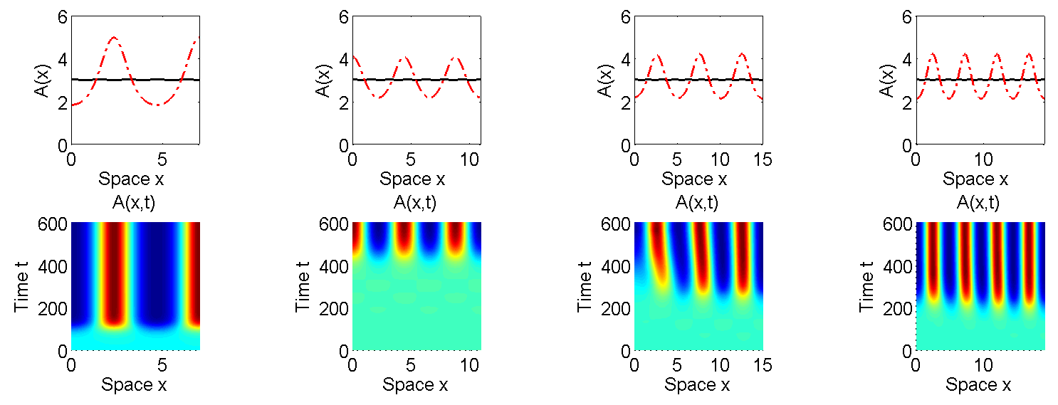
Domain size L𝐿L 3 5 7 9 11
Model (1.2) k0subscript𝑘0k_{0} 1 2 3 4 5
ϵ¯k0(1.2)subscriptsuperscript¯italic-ϵ1.2subscript𝑘0\bar{\epsilon}^{(\ref{12})}_{k_{0}} 0.0781 0.1004 0.1003 0.0991 0.0981
Model (1.3) k0subscript𝑘0k_{0} 1 2 3 4 5
ϵ¯k0(1.3)subscriptsuperscript¯italic-ϵ1.3subscript𝑘0\bar{\epsilon}^{(\ref{13})}_{k_{0}} 0.0963 0.1239 0.1238 0.1224 0.1221
Domain size L𝐿L 13 15 17 19 21
Model (1.2) k0subscript𝑘0k_{0} 5 6 7 8 9
ϵ¯k0(1.2)subscriptsuperscript¯italic-ϵ1.2subscript𝑘0\bar{\epsilon}^{(\ref{12})}_{k_{0}} 0.0988 0.1004 0.1008 0.1006 0.1001
Model (1.3) k0subscript𝑘0k_{0} 5 6 7 8 9
ϵ¯k0(1.3)subscriptsuperscript¯italic-ϵ1.3subscript𝑘0\bar{\epsilon}^{(\ref{13})}_{k_{0}} 0.1219 0.1239 0.1243 0.1242 0.1238
Table 2: Wavemode number that maximizes the bifurcation value for different intervals. We see that system (4.1) and (4.2) have the same wavemode number, which increases as domain size increases. The first bifurcation value maxkN+ϵ¯ksubscript𝑘superscript𝑁subscript¯italic-ϵ𝑘\max_{k\in{N}^{+}}\bar{\epsilon}_{k} of system (1.2) is smaller than that of system (1.3).
Refer to caption
Figure 3: Emergence of stable multi-spike steady states to model (1.2) with domain size L=7𝐿7L=7, 11, 15 and 19 from the left to the right. Initial condition is plotted in solid curve and steady state in dash-dotted lines. Parameters are A0=1superscript𝐴01A^{0}=1, B¯=2¯𝐵2\bar{B}=2, λ=0.1𝜆0.1\lambda=0.1 and ϵ=0.09italic-ϵ0.09\epsilon=0.09. According to our theoretical results and Table 2, the wavemodes are cos3πx73𝜋𝑥7\cos\frac{3\pi x}{7}, cos5πx115𝜋𝑥11\cos\frac{5\pi x}{11}, cos6πx156𝜋𝑥15\cos\frac{6\pi x}{15} and cos8πx198𝜋𝑥19\cos\frac{8\pi x}{19}, respectively. Plots in this figure verify this exact wavemode selection mechanism.

6.1.2 Effect of small diffusion rate ϵitalic-ϵ\epsilon

In Figure 4, we plot the steady state of (1.2) over (0,1)01(0,1) for ϵ>0italic-ϵ0\epsilon>0 being sufficiently smaller than the maximum bifurcation value ϵk0subscriptitalic-ϵsubscript𝑘0\epsilon_{k_{0}}, where all the rest parameters and initial data are taken to be the same as those in Figure 2. Our numerical simulations show that both A(x)𝐴𝑥A(x) and ρ(x)𝜌𝑥\rho(x) are monotone decreasing for ϵitalic-ϵ\epsilon being small. Moreover as ϵitalic-ϵ\epsilon shrinks to zero, steady state A(x)𝐴𝑥A(x) approaches to a boundary spike in the form of a δ𝛿\delta-function and ρ(x)𝜌𝑥\rho(x) to a boundary spike with bounded maximum value. This result indicates that if the nearby victimization effect is extremely weak, one may expect the emergence of the clusterings of crime data. However, rigorous analysis of the spiky solution is a quite delicate problem and it is out of the scope of our paper. See [26] for mathematical analysis on spiky solutions of (1.1) for instance.
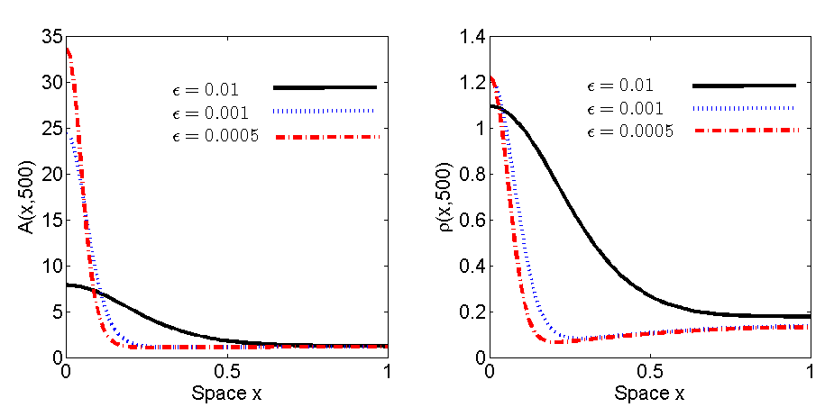
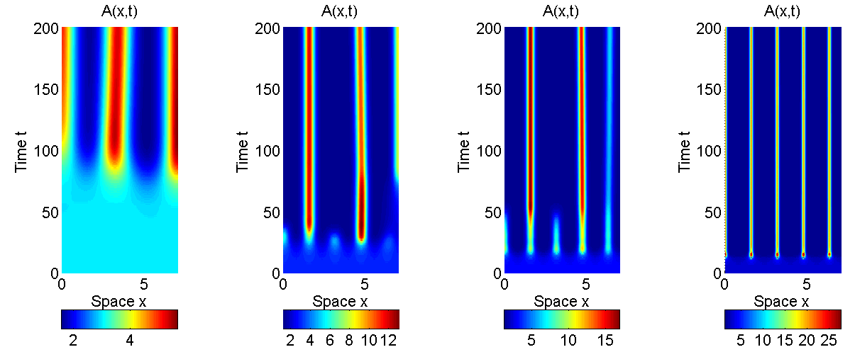
Refer to caption
Figure 4: Plots of stable boundary spikes for small diffusion rate ϵitalic-ϵ\epsilon. Our numerical solutions suggest that as ϵitalic-ϵ\epsilon shrinks to zero A(x)𝐴𝑥A(x) converges to a δ𝛿\delta-type boundary spike and ρ(x)𝜌𝑥\rho(x) converges to a bounded boundary spike.
Refer to caption
Figure 5: Formation of stable spikes of model (1.2) for different values of ϵitalic-ϵ\epsilon, which is taken to be 0.05, 0.01, 0.005 and 0.001 in each plot from the left to the right respectively. Number of aggregates increases as ϵitalic-ϵ\epsilon shrinks to zero.

6.1.3 Difference between model (1.2) and model (1.3)

Next we compare the pattern formations in the departure–dependent system (1.2) and the arrival–dependent system (1.3). We want to remind that both systems admit (A¯,ρ¯)¯𝐴¯𝜌(\bar{A},\bar{\rho}) as their homogeneous steady state solutions. To elucidate their differences, we choose the same parameters and initial data for both systems as those for Figure 3. We remind that, according to Table 2, both models have the same wavemode number k0subscript𝑘0k_{0} which increases as domain size L𝐿L increases. On the other hand, the first bifurcation value maxkN+ϵ¯ksubscript𝑘superscript𝑁subscript¯italic-ϵ𝑘\max_{k\in{N}^{+}}\bar{\epsilon}_{k} of (1.2) is always smaller than that of system (1.3), therefore (A¯,ρ¯)¯𝐴¯𝜌(\bar{A},\bar{\rho}) loses its stability in (1.2) for smaller value of ϵitalic-ϵ\epsilon than (1.3). This suggests that, in light of simulations in Figure 4, (1.3) can develop spikes which have larger amplitudes than (1.2) for each fixed small ϵitalic-ϵ\epsilon. This is numerically illustrated in Figure 6, where we select ϵitalic-ϵ\epsilon to be far away from the ϵ¯k0subscript¯italic-ϵsubscript𝑘0\bar{\epsilon}_{k_{0}}.

Refer to caption
Figure 6: Stable steady states of systems (1.2) and (1.3) for different values of ϵitalic-ϵ\epsilon. Steady states of the departure–dependent model (1.2) are given in dotted blue lines and steady states of the arrival–dependent model (1.3) are given in dash–dotted red lines. The amplitude of spikes of model (1.2) is always larger than those of model (1.3). This suggests that the arrival–dependent model (1.3) is more sensitive to the variation of near repeat victimization effect ϵitalic-ϵ\epsilon than the departure–dependent model (1.2). This is consistent with the linear stability results in Section 3. For ϵitalic-ϵ\epsilon being sufficiently small, both models have the same structures in their stable steady states; moreover, the stable patterns no longer fall into the category of our wavemode selection mechanism.

In Figure 6, we numerically solve system (1.2) and system (1.3) over (0,10)010(0,10) for different values of ϵitalic-ϵ\epsilon. Parameters are chosen to be A0=1superscript𝐴01A^{0}=1, B¯=3¯𝐵3\bar{B}=3 and the initial data are A0(x)=A¯+0.01cosπx4subscript𝐴0𝑥¯𝐴0.01𝜋𝑥4A_{0}(x)=\bar{A}+0.01\cos\frac{\pi x}{4} and ρ0(x)=ρ¯+0.01cos2πxsubscript𝜌0𝑥¯𝜌0.012𝜋𝑥\rho_{0}(x)=\bar{\rho}+0.01\cos 2\pi x. There are several conclusions that we can draw out of Figure 6. First of all, the numerical simulations there verify that system (1.2) and (1.3) have the same wavemode section mechanism which is consistent with our theoretical analysis above. See Table 2 and the discussions there for example. Moreover, the amplitude of patterns to (1.2) is larger than that of (1.3), while both systems have the same stable steady states for ϵitalic-ϵ\epsilon being sufficiently small. We can also find that small ϵitalic-ϵ\epsilon tends to support the formation of stable steady states with spikes and amplitude of each spike increases as ϵitalic-ϵ\epsilon goes to zero.

6.1.4 Merging and emerging of interior spikes

In Figure 7, we observe the merging of spikes of house attractiveness for model (1.2) in plot (a) and the emerging of new spikes for model (1.3 in plot (b)). These patterning processes are referred to as coarsening processes which have been observed in chemotaxis model with logistic growth in [31]. In plot (a), we choose ϵ=0.026italic-ϵ0.026\epsilon=0.026, A0=1superscript𝐴01A^{0}=1, B¯=9.11¯𝐵9.11\bar{B}=9.11 and λ=0.1𝜆0.1\lambda=0.1. Initial data are (A0(x),ρ0(x)=(A¯,ρ¯)+(0.001,0.001)cos(1.2πx)(A_{0}(x),\rho_{0}(x)=(\bar{A},\bar{\rho})+(0.001,0.001)\cos(1.2\pi x). We observe that two spikes merge to form a single spike at around x=8𝑥8x=8 and x=13𝑥13x=13. In plot (b), we choose ϵ=0.03italic-ϵ0.03\epsilon=0.03, A0=0.967subscript𝐴00.967A_{0}=0.967, B¯=13.09¯𝐵13.09\bar{B}=13.09 and λ=0.1𝜆0.1\lambda=0.1. Initial data are (A0(x),ρ0(x)=(A¯,ρ¯)+(0.0007,0.0007)cos(0.3πx)(A_{0}(x),\rho_{0}(x)=(\bar{A},\bar{\rho})+(0.0007,0.0007)\cos(0.3\pi x). We observe that two spikes emerge from a single spike at around x=8𝑥8x=8 and x=17.5𝑥17.5x=17.5. Shifting of spikes is observed in both figures. Our numerical simulations also suggest that there is usually no coarsening when the domain size is small, which often occurs when domain size and A¯¯𝐴\bar{A} are large.

Refer to caption
Figure 7: Merging and emerging of spikes. In Figure (a) and Figure (b), we plot the merging and emerging of spikes to system (1.2) and system (1.3) respectively.

6.2 2D numerics

We now study models (1.2) and (1.3) over the two-dimensional domain Ω=(0,L)×(0,L)Ω0𝐿0𝐿\Omega=(0,L)\times(0,L). In this special case, the Neumann eigen-pairs are

(mπL)2+(mπL)2cosmπxLcosnπyL,(m,n)N+×N+{(1,0),(0,1)}.superscript𝑚𝜋𝐿2superscript𝑚𝜋𝐿2𝑚𝜋𝑥𝐿𝑛𝜋𝑦𝐿𝑚𝑛superscript𝑁superscript𝑁1001\Big{(}\frac{m\pi}{L}\Big{)}^{2}+\Big{(}\frac{m\pi}{L}\Big{)}^{2}\leftrightarrow\cos\frac{m\pi x}{L}\cos\frac{n\pi y}{L},(m,n)\in{N}^{+}\times{N}^{+}\cup\{(1,0),(0,1)\}.

According to Theorem 4.1 and Theorem 4.2, each eigenvalue above gives rise to a bifurcation value for models (1.2) and (1.3) when the Laplace eigen–value is simple. However out simulations here indicates that these results hold even in the case when ΩΩ\Omega is a square for which the eigen–value is not simple. We also want to point out that the boundary of the square is not smooth at the corners, therefore the Neumann boundary condition and the bifurcation solutions can be interpreted as the weak solutions through the first Green’s identity. One can show that the weak solutions are classical except at the corners by elliptic embeddings in the standard way.

Bifurcation values ϵ¯mnsubscript¯italic-ϵ𝑚𝑛\bar{\epsilon}_{mn}
m=0𝑚0m=0 m=1𝑚1m=1 m=2𝑚2m=2 m=3𝑚3m=3 m=4𝑚4m=4 m=5𝑚5m=5
n=0𝑛0n=0 undefined 0.0094 0.0091 0.0047 0.0028 0.0019
n=1𝑛1n=1 0.0094 0.0129 0.0077 0.0043 0.0027 0.0018
n=2𝑛2n=2 0.0091 0.0077 0.0053 0.0034 0.0023 0.0016
n=3𝑛3n=3 0.0047 0.0043 0.0034 0.0025 0.0019 0.0014
n=4𝑛4n=4 0.0028 0.0027 0.0023 0.0019 0.0015 0.0012
n=5𝑛5n=5 0.0019 0.0018 0.0016 0.0014 0.0012 0.0009
Table 3: List of bifurcation values ϵ¯mnsubscript¯italic-ϵ𝑚𝑛\bar{\epsilon}_{mn} in (4.7) for system (1.2) over Ω=(0,1)×(0,1)Ω0101\Omega=(0,1)\times(0,1). Parameters are taken to be A0=1superscript𝐴01A^{0}=1, B¯=3¯𝐵3\bar{B}=3 and λ=0.9𝜆0.9\lambda=0.9. We see that ϵ¯11=maxϵ¯mnsubscript¯italic-ϵ11subscript¯italic-ϵ𝑚𝑛\bar{\epsilon}_{11}=\max\bar{\epsilon}_{mn} and the stable wavemode is cosπxcosπy𝜋𝑥𝜋𝑦\cos\pi x\cos\pi y.

6.2.1 Effect of domain size on wavemode selection mechanism

In Figure 8, we plot the numerical solutions of system (1.2) over the 2D domain Ω=(0,1)×(0,1)Ω0101\Omega=(0,1)\times(0,1) to illustrate our result in Table 3. The parameters are chosen to be A0=1superscript𝐴01A^{0}=1, B¯=3¯𝐵3\bar{B}=3 and λ=0.9𝜆0.9\lambda=0.9. The initial conditions are taken to be small perturbations from the homogeneous steady state (A¯,ρ¯)¯𝐴¯𝜌(\bar{A},\bar{\rho}).

Refer to caption
Figure 8: Formation of double-spike steady state. We choose the parameters to be ϵ=0.008italic-ϵ0.008\epsilon=0.008, A0=1superscript𝐴01A^{0}=1, B¯=3¯𝐵3\bar{B}=3 and λ=0.9𝜆0.9\lambda=0.9. Stable generating wavemode is cosπxcosπy𝜋𝑥𝜋𝑦\cos\pi x\cos\pi y. The formation of stable steady state corresponds to the wavemode selection as in our analysis.

According to our theoretical results, the stable wavemode of (1.2) over Ω=(0,L)×(0,L)Ω0𝐿0𝐿\Omega=(0,L)\times(0,L) must be cosm0πxLcosn0πyLsubscript𝑚0𝜋𝑥𝐿subscript𝑛0𝜋𝑦𝐿\cos\frac{m_{0}\pi x}{L}\cos\frac{n_{0}\pi y}{L} for which (m0,n0)(0,0)subscript𝑚0subscript𝑛000(m_{0},n_{0})\neq(0,0) maximizes ϵ¯m0n0subscript¯italic-ϵsubscript𝑚0subscript𝑛0\bar{\epsilon}_{m_{0}n_{0}} in (4.7), with σksubscript𝜎𝑘\sigma_{k} being replaced by (mπL)2+(mπL)2superscript𝑚𝜋𝐿2superscript𝑚𝜋𝐿2\big{(}\frac{m\pi}{L}\big{)}^{2}+\big{(}\frac{m\pi}{L}\big{)}^{2}. Models (1.2) and (1.3) admit nontrivial patterns that develop in form of this mode if ϵitalic-ϵ\epsilon is around ϵ¯m0n0subscript¯italic-ϵsubscript𝑚0subscript𝑛0\bar{\epsilon}_{m_{0}n_{0}}. Similar as in 1D, by periodically reflecting and extending hotspot at the boundary of square (0,L)×(0,L)0𝐿0𝐿(0,L)\times(0,L), we can construct steady states with more spikes to larger domains (0,mL)×(0,nL)0𝑚𝐿0𝑛𝐿(0,mL)\times(0,nL), (m.n)N+×N+(m.n)\in{N}^{+}\times{N}^{+}. This observation suggests that large domain supports more hotspots than small domain. Actually, we can verify this by our wavemode section mechanism. Table 4 gives the wavemode series for a list of square domains with different side lengths.

Domain size L𝐿L 2 3 4 5 6 7 8 9
Model (1.2) (m0,n0)subscript𝑚0subscript𝑛0(m_{0},n_{0}) (2,2) (4,0), (0,4) (1,5), (5,1) (4,5), (5,4) (3,7), (7,3) (4,8), (8,4) (2,10), (10,2) (7,9), (9,7)
ϵ¯m0,n0(1.2)subscriptsuperscript¯italic-ϵ1.2subscript𝑚0subscript𝑛0\bar{\epsilon}^{(\ref{12})}_{m_{0},n_{0}} 0.0129 0.0132 0.0133 0.0133 0.0133 0.0133 0.0133 0.0133
Model (1.3) (m0,n0)subscript𝑚0subscript𝑛0(m_{0},n_{0}) (2,2) (4,0), (0,4) (1,5), (5,1) (4,5), (5,4) (3,7), (7,3) (4,8), (8,4) (2,10), (10,2) (7,9), (9,7)
ϵ¯(m0,n0)(1.3)subscriptsuperscript¯italic-ϵ1.3subscript𝑚0subscript𝑛0\bar{\epsilon}^{(\ref{13})}_{(m_{0},n_{0})} 0.0145 0.0148 0.0149 0.0149 0.0149 0.0149 0.0149 0.0149
Table 4: Wavemode number that maximizes the bifurcation value ϵ¯mnsubscript¯italic-ϵ𝑚𝑛\bar{\epsilon}_{mn} of systems (1.2) and (1.3) for different values of domain size L𝐿L. The parameters are taken to be A0=1superscript𝐴01A^{0}=1, B¯=3¯𝐵3\bar{B}=3 and λ=0.9𝜆0.9\lambda=0.9. We see that model (1.2) and (1.3) have the same wavemode selection mechanism. Moreover, the increase in domain size decreases the maximum bifurcation values for both models. Complex patterns with aggregates usually emerge for large domains.
Refer to caption
Figure 9: Stable hotspots to house attractiveness and criminal density of model (1.2) for different values of domain size. We choose the parameters to be ϵ=0.00127italic-ϵ0.00127\epsilon=0.00127, A0=1superscript𝐴01A^{0}=1, B¯=3¯𝐵3\bar{B}=3 and λ=0.9𝜆0.9\lambda=0.9. The initial conditions are taken to be A0(x,y)=A¯+0.01cosπxsubscript𝐴0𝑥𝑦¯𝐴0.01𝜋𝑥A_{0}(x,y)=\bar{A}+0.01\cos\pi x and ρ0(x,y)=ρ¯+0.01cosπx4subscript𝜌0𝑥𝑦¯𝜌0.01𝜋𝑥4\rho_{0}(x,y)=\bar{\rho}+0.01\cos\frac{\pi x}{4}. According to our theoretical results and Table 4, the wavemodes are cos4πx34𝜋𝑥3\cos\frac{4\pi x}{3}, cos4πx5cos5πy54𝜋𝑥55𝜋𝑦5\cos\frac{4\pi x}{5}\cos\frac{5\pi y}{5}, cos4πx7cos8πy74𝜋𝑥78𝜋𝑦7\cos\frac{4\pi x}{7}\cos\frac{8\pi y}{7} and cos7πx9cos9πy97𝜋𝑥99𝜋𝑦9\cos\frac{7\pi x}{9}\cos\frac{9\pi y}{9} respectively. Stable steady states correspond to these wavemodes and verify selection mechanism in 2D.

6.2.2 Effect of small diffusion rate ϵitalic-ϵ\epsilon

Finally, we study in Figure 10 the qualitative behaviors of stationary hotspots to model (1.2) for ϵitalic-ϵ\epsilon being greatly smaller than its maximum bifurcation point ϵ¯m0n0subscript¯italic-ϵsubscript𝑚0subscript𝑛0\bar{\epsilon}_{m_{0}n_{0}}. The parameters are taken to be the same as those in Figure 9. Similar as in the 1D case, our numerical simulations suggest that small diffusion rate ϵitalic-ϵ\epsilon increases the number of stable hotspots and the magnitude of the aggregates.

Refer to caption
Figure 10: Stable hotspots to house attractiveness as diffusion rate ϵitalic-ϵ\epsilon shrinks to zero. We surmise that A(x,y)𝐴𝑥𝑦A(x,y) converges to a linear combination of δ𝛿\delta-functions as ϵitalic-ϵ\epsilon goes to zero. Stable hotspots are also observed in the criminal population density.

7 Conclusions and Discussions

In this paper, we study the stationary solutions to the general 2×2222\times 2 reaction–diffusion models (1.2) and (1.3) over multi-dimensional bounded domains subject to homogeneous Neumann boundary conditions. These systems are generalizations of the urban crime model proposed by Short et al. Our modification is made based on the assumption that both the near–repeat victimization effect and perception of attractiveness are heterogeneous, i.e., dependent on the attractiveness of its current and/or neighbouring sites.

First of all, we carry out the linear stability analysis of the homogenous equilibrium (A¯,ρ¯)¯𝐴¯𝜌(\bar{A},\bar{\rho}). It is shown that this trivial solution loses its stability when the intrinsic near–repeat victimization effect ϵitalic-ϵ\epsilon becomes large. Then we proceed to investigate the existence of nonhomogeneous steady state that bifurcates from the homogeneous steady state in the manner of Crandall–Rabinowitz local bifurcation theory. Moreover, we perform the stability analysis of these nontrivial patterns by detailed calculations. Compared to the bifurcation analysis in [8], our results treat a wider class of urban crime models; moreover, we find the exact formula of K2subscript𝐾2K_{2} for the pitch-fork bifurcation when K1=0subscript𝐾10K_{1}=0, which was not done in [8].

Our stability results provide a selection mechanism of principal wavemode in the formations of nontrivial patterns. To be precise, the only stable wavemode must be a Neumann eigenfunction Φk0subscriptΦsubscript𝑘0\Phi_{k_{0}}, whose wavemode number k0subscript𝑘0k_{0} is a positive integer that maximizes the bifurcation value ϵ¯ksubscript¯italic-ϵ𝑘\bar{\epsilon}_{k} over positive integers; moreover, the pattern (Ak(s,x),ρk(s,x))subscript𝐴𝑘𝑠𝑥subscript𝜌𝑘𝑠𝑥(A_{k}(s,x),\rho_{k}(s,x)) is unstable for all kk0𝑘subscript𝑘0k\neq k_{0}. Based on the stable wavemode selection mechanism, we can precisely predict the formation of stable patterns of the house attractiveness and criminal population density that have large amplitude such as boundary spikes, interior spikes in 1D and hotspots and hotstripes in 2D.

Numerical simulations have been performed to verify our theoretical results when the domain is a one–dimensional interval or a two–dimensional square. There are also several important findings in our numerics. First of all, they indicate that both small diffusion rate ϵitalic-ϵ\epsilon and large domain size support the emergence of stable aggregates. Moreover, the amplitude of house attractiveness A(x)𝐴𝑥A(x) and criminal population density ρ(x)𝜌𝑥\rho(x) increase as ϵitalic-ϵ\epsilon decreases. In particular, A(x)𝐴𝑥A(x) approaches to a δ𝛿\delta-type function as ϵitalic-ϵ\epsilon shrinks to zero. These results suggest that small nearby victimization effect tends to support the clustering of criminal data, and urban regions have much more complicated criminal behaviors than small rural areas. We also observe that coarsening process ocuurs where two spikes merging into one new spike or one spike breaking into two separate spikes, in 1D simulations.

There are also some other unsolved questions concerning the stationary solutions of models (1.2) and (1.3). Theorem 4.1, 4.2 and Theorem 5.1 give us the existence and stability of their nontrivial positive steady states, which are small perturbation from the homogeneous equilibrium. It is interesting to investigate the emergence of large amplitude solutions such as the spikes and hotspots demonstrated in our numerical simulations. Another interesting but delicate problem is to investigate the stability of these aggregates. Our bifurcation analysis is performed based on the local theory of [12] and it is interesting and important to study its global continuums when ϵitalic-ϵ\epsilon is away from the bifurcation point ϵ¯ksubscript¯italic-ϵ𝑘\bar{\epsilon}_{k}. According to Remark 4.1, for each bifurcation branch, one has to determine whether its continuum is noncompact, i.e., approaches to infinity, or intersects the ϵitalic-ϵ\epsilon–axis at ϵsuperscriptitalic-ϵ\epsilon^{*}, which should not one of the bifurcation values. However, this can be a quite challenging problem even over one–dimensional domains.

When ϵitalic-ϵ\epsilon is chosen to be close to the principal bifurcation value maxkN+ϵ¯ksubscript𝑘superscript𝑁subscript¯italic-ϵ𝑘\max_{k\in{N}^{+}}\bar{\epsilon}_{k}, our wavemode selection mechanism provides a very useful and effective way to predict the formation of spikes and hotspots in systems (1.2) and (1.3). However, when ϵitalic-ϵ\epsilon is far away from the principal bifurcation value, i.e., being sufficiently small, rigorous mathematical analysis of the dynamics of the aggregates is needed to fully understand the pattern formation in these models. For example, the mechanism that drives the merging and emerging of spikes in Figure 7 is a delicate question that deserves future explorations. From the viewpoint of mathematical analysis, it is also important to investigate dynamics of the time-dependent systems (1.2) and (1.3), including but not limited to questions such as global existence, convergence to the steady states, traveling wave solutions, etc.

References

  • [1] L. Anselin, J. Cohen, D. Cook, W. Gorr and G. Tita, Spatial analysis of crime, Criminal Justice, 4 (2000), 212–262.
  • [2] L. Bettencourt, J. Lobo, D. Strumsky and G. West, Urban scaling and its deviations: Revealing the structure of wealth, innovation and crime across cities, PLOS one., 5 (2010),
  • [3] H. Berestycki, N. Rodriguez and L. Ryzhik, Traveling wave solutions in a reaction–diffusion model for criminal activity, Multiscale Model. Simul., 11 (2013), 1097–1126.
  • [4] A. Bottoms and P. Wiles, Crime, policing and places: Essay in environmental criminology, Routledge, (1992), 27–54.
  • [5] P. Brantingham, Crime pattern, McMillan, 1987.
  • [6] P. Brantingham, Freight train graffiti: Subculture, crime, dislocation, Justice Quarterly, 15 (1998), 587–608.
  • [7] P. Brantingham, Domestic burglary repeats and space-time clusters the dimensions of risk, European Journal of Criminology, 2 (2005), 67–92.
  • [8] R. Cantrell, C. Cosner and R. Manásevich, Global bifurcation of solutions for crime modeling equations, SIAM J. Math. Anal., 44, (2012), 1340–1358.
  • [9] W. Chambliss, Functional and conflict theories of crime, MSS Modular Publications 1973.
  • [10] S. Chaturapruek, J. Breslau, D. Yazdi, T. Kolokolnikov and S. McCalla, Crime modeling with Lévy flights, SIAM J. Appl. Math., 73 (2013), 1703–1720.
  • [11] S. Cohn, S. Barkan and W. Halteman, Punitive attitudes toward criminals: racial consensus or racial conflict, Soc. Probs, 38 (1991), 287–296.
  • [12] M. Crandall and P. Rabinowitz, Bifurcation from simple eigenvalues, J. Funct. Anal., 8 (1971) 321–340.
  • [13] M. Crandall and P. Rabinowitz, Bifurcation, perturbation of simple eigenvalues, and linearized stability, Arch. Rational Mech. Anal., 52 (1973) 161–180.
  • [14] A.-K. Drangeid, The principle of linearized stability for quasilinear parabolic evolution equations, Nonlinear Anal., 13 (1989) 1091–1113.
  • [15] D. Horstmann, From 1970 until now: the Keller-Segel model in chemotaxis and its consequences I, Jahresber DMV, 105 (2003), 103–165.
  • [16] D. Lloyd, H. OFarrell, On localised hotspots of an urban crime model, Phys. D, 253 2013, 23–39.
  • [17] R. Manásevich, M. Garcia–Huidobro and J. Mawhin, Existence of solutions for a 1-D boundary value problem coming from a model for burglary, Nonlinear Anal. Real World Appl., 15 (2013), 1939–-1946.
  • [18] M. Garcia–Huidobro, R. Manásevich and J. Mawhin, Solvability of a nonlinear Neumann problem for systems arising from a burglary model, Appl. Math. Lett., 35 (2014), 102–108.
  • [19] T. Hillen, K. Painter, A user’s guidence to PDE models for chemotaxis, J. Math. Biol., 58 (2009), 183–217.
  • [20] P. Jones, P. Brantingham and L. Chayes, Statistical models of criminal behavior: the effects of law enforcement actions, Math. Models Methods Appl. Sci., 20, (2010) 1397–1423.
  • [21] S. Johnson, K. Bowers and A. Hirschfield, New insights into the spatial and temporal distribution of repeat victimization, British Journal of Criminology, 37 (1997) 224–241.
  • [22] E. F. Keller and L. A. Segel, Inition of slime mold aggregation view as an instability, Journal of Theoratical Biology, 26 (1970), 399–415.
  • [23] E. F. Keller and L. A. Segel, Model for chemotaxis, Journal of Theoratical Biology, 30 (1971), 225–234.
  • [24] [10.1016/0022-5193(71)90051-8] E. F. Keller and L. A. Segel, Traveling bands of chemotactic bacteria: A Theretical Analysis, Journal of Theoratical Biology, 30 (1971), 235–248.
  • [25] T. Kato, ”Functional Analysis”, Springer Classics in Mathematics, (1996).
  • [26] T. Kolokolnikov, M. Ward and J. Wei, The stability of steady–state hot-spot patterns for a reaction–diffusion model of urban crime, Discrete Contin. Dyn. Syst. Ser. B, 19 (2014), 1373–1410.
  • [27] C. E. Kubrin and R. Weitzer, New directions in social disorganization theory, Journal of Research in Crime and Delinquency, 40 (2003), 374–402.
  • [28] M. Ma, C. Ou, and Z. Wang, Stationary solutions of a volume filling chemotaxis model with logistic growth, SIAM J. Appl. Math., 72 (2012), 740–766.
  • [29] R. Manásevich, Q. Phan and P. Souplet, Global existence of solutions for a chemotaxis-type system arising in crime modelling, European J. Appl. Math., 24 (2013), 273–296.
  • [30] Y. Nec, M. Ward, The stability and slow dynamics of two-spike patterns for a class of reaction–diffusion system, Math. Model. Nat. Phenom., 8 (2013), 206–232.
  • [31] K. Painter and T. Hillen, Spatio–temporal chaos in a chemotaxis model, 240 (2011), Phys. D, 363–375.
  • [32] M. Perc, K. Donnay and D. Helbing, Understanding recurrent crime as system–immanent collective behavior, 8 (2013), PLOS one.
  • [33] R. D. Peterson and L.J. Krivo, Racial segregation and black urban homicide, Social Forces., 71 (1993), 1001–1026.
  • [34] L. Ricketson, A continuum model of residential burglary incorporating law enforcement, preprint.
  • [35] N. Rodriguez, On the global well-posedness theory for a class of PDE models for criminal activity, Phys. D, 260 (2013), 191–200.
  • [36] N. Rodriguez and A. Bertozzi, Local existence and uniqueness of solutions to a PDE model of criminal behavior, Math. Models Methods Appl. Sci., special issue on Mathematics and Complexity in Human and Life Sciences, 20 (2010), 1425–1457.
  • [37] N. Rodriguez and L. Ryzhik, Exploring the effects of social preference, economic disparity, and the environment on segregation, Commun. Math. Sci., 14 (2016), 363–387.
  • [38] R. Sampson and W. B. Groves, Community structure and crime: testing social–disorganization theory, American Journal of Sociology, 94 (1989), 774–802.
  • [39] R. Sampson and S. Raudenbush, Seeing disorder: neighborhood stigma and the social construction of ”croken windows”, Social Psychology Quarterly, 67 (2004), 319–342.
  • [40] J. Shi and X. Wang, On global bifurcation for quasilinear elliptic systems on bounded domains, J. Differential Equations, 246 (2009), 2788–2812.
  • [41] M. Short, A. Bertozzi and P. Brantingham, Nonlinear patterns in urban crime: Hotspots, bifurcations, and suppression, SIAM, J. Appl. Dyn. Syst., 9 (2010), 462–483.
  • [42] M. Short, G. Mohler, P. Brantingham and G. Tita, Gang rivalry dynamics via coupled point process networks, Discrete Contin. Dyn. Syst. Ser. B, 19 (2014), 1459–1477.
  • [43] M. Short, M. DOrsogna, V. Pasour, G. Tita, P. Brantingham, A. Bertozzi and L. Chayes, A statistical model of criminal behavior, Math. Models Methods Appl. Sci., 18 (2008), 1249-1267.
  • [44] B. Sleeman, M. Ward and J. Wei, The existence and stability of spike patterns in a chemotaxis model, SIAM J. Appl. Math., 65 (2005), 790–817.
  • [45] S. Tse, M. Ward, Hotspot formation and dynamics for a continuum model of urban crime, Europ. J. Appl. Math., to appear.
  • [46] J. Wilson and G. Kelling, ”Broken Windows: The police and neighborhood safety”, The Atlantic, 1982
  • [47] M. Wolfgang and F. Ferracuti, ”Subculture of violence-towards an integrated theory in criminology”, 406, Sage Publications, Inc.
  • [48] J. Woodworth, G. Mohler, A. Bertozzi and P. Brantingham, Nonlocal crime density estimation incorporating housing information, Philos. Trans. R. Soc. Lond. Ser. A Math. Phys. Eng. Sci., 372 (2014), 15 pp.
  • [49] J. Zipkin, M. Short and A. Bertozzi, Cops on the dots in a mathematical model of urban crime and police response, Discrete Contin. Dyn. Syst. Ser. B, 19 (2014), 1479–1506.