Spin transport with traps: dramatic narrowing of the Hanle curve

Abstract

We study theoretically the spin transport in a device in which the active layer is an organic film with numerous deep in-gap levels serving as traps. A carrier, diffusing between magnetized injector and detector, spends a considerable portion of time on the traps. This new feature of transport does not affect the giant magnetoresistance, which is sensitive only to the mutual orientation of magnetizations of the injector and detector. By contrast, the presence of traps strongly affects the sensitivity of the spin transport to external magnetic field perpendicular to the magnetizations of the electrodes (the Hanle effect). Namely, the Hanle curve narrows dramatically. The origin of such a narrowing is that the spin precession takes place during the entire time of the carrier motion between the electrodes, while the spin relaxation takes place only during diffusive motion between the subsequent traps. If the resulting width of the Hanle curve is smaller than the measurement resolution, observation of the Hanle peak becomes impossible.

I Introduction

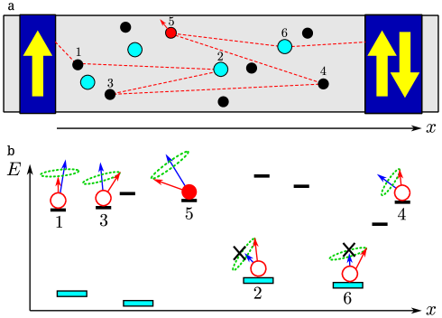
Figure 1: (Color Online). Carrier transport between the magnetized electrodes in the presence of deep traps is illustrated schematically in coordinate (a) and energy (b) spaces. An injected spin-up carrier relaxes the spin while visiting the sites numbered as $1$, $3$, $4$, and $5$, but preserves the spin while visiting the traps numbered as $2$ and $6$.

Observation of the giant magnetoresistance (GMR) effect in organic devicesOrganicValve1 ; OrganicValve1' was later reproduced by many groups on various organic active layers and with various ferromagnetic electrodes, see e.g. Refs. Valve1, ; Valve2, ; Valve3, ; Valve4, ; Valve5, ; Valve6, . Along with demonstration of GMR, the value of spin diffusion length in organic film, $\lambda_{s}=40$nm, was inferred in Ref. OrganicValve1', from the thickness dependence of the effect. This value is by a factor of $\sim 20$ smaller than $\lambda_{s}$ in a number of conventional semiconductors, see e.g. Refs. Conventional1, ; Conventional2, ; Conventional3, . These and many other papers where the GMR effect is reported, also report the observation of the Hanle effect. It is the latter observation which constitutes an unambiguous proof that the actual spin transport between the electrodes takes place. The Hanle effect manifests itself as a drop of the resistance of the structure with channel length, $L\sim\lambda_{s}$, as the external field normal to the magnetizations of the electrodes is applied. This drop is the result of the Larmor precession of spins of the injected carriers.

Despite indirect indicationsInjectionYes1 ; InjectionYes2 ; InjectionYes3 of a finite spin polarization in the active layer, the Hanle effect in organic devices is either completely missingNoInjection1 ; NoInjection2 ; NoInjection3 or shows up as a weak signatureHanleOrganicJapanese1 ; HanleOrganicJapanese2 . In experimental papers Refs. NoInjection1, ; NoInjection2, ; NoInjection3, , the puzzling absence of the Hanle effect was ascribed to a strong inhomogeneity of either organic layer itselfNoInjection1 ; NoInjection2 or of the electrodesNoInjection3 . In a theoretical paper, Ref. Yu, , the explanation of the “missing” Hanle effect dwells upon a presumed specific property of organic materials, namely, strong exchange coupling between carriers which leads to anomalously short spin diffusion time, $\tau_{s}$. According to Ref. Yu, , short $\tau_{s}$ requires very strong magnetic fields to reveal the spin precession. In other words, the explanation of the absence of the Hanle effect is that the Hanle curve is too broad.

In the present paper we exploit a different intrinsic property of organic semiconductors which distinguishes them from the conventional crystalline semiconductors. This property is the presence of deep traps, see Fig. 1, which a carrier visits on the way between the injector and detector. Our only assumption about these traps is that, while sitting on a trap, a carrier is not subject to spin relaxation. From this assumption we readily derive that, while the GMR response is unaffected by traps, the Hanle effect is affected dramatically. Namely, as a result of visiting the traps, the Hanle curve narrows. This scenario, although opposite to Ref. Yu, , also inhibits the observability of the Hanle effect. The effect will not be detectable if the width of the Hanle curve is smaller than the measurement resolution.

A toy model. To illustrate our message, consider a toy model of GMR in organicsmultistep1 ; multistep2 illustrated in Fig. 2. The current between the electrodes is due to a sequential hopping via only two intermediate states, ${\cal T}$ and ${\cal S}$. Denote with ${\bm{B}}_{\scriptscriptstyle{\cal S}}$ and ${\bm{B}}_{\scriptscriptstyle{\cal T}}$ the on-site fields in which the carrier spin precesses while waiting for the hop. The advantage of this model is that the Hanle signal, defined asSilsbee1988 ; vanWeesPioneering ; Crowell2007

$$R_{H}\propto\int_{0}^{\infty}dtS_{z}(t),$$ (1)

can be calculated explicitly. With two steps, the expression for $R_{H}$ can be cast in the form

$$R_{H} =C_{2}\int\limits_{0}^{\infty}dt_{\scriptscriptstyle{\cal S}}f_{\scriptscriptstyle{\cal S}}(t_{\scriptscriptstyle{\cal S}})\int\limits_{0}^{\infty}dt_{\scriptscriptstyle{\cal T}}f_{\scriptscriptstyle{\cal T}}(t_{\scriptscriptstyle{\cal T}})$$

$$\times\left\{\left|\left<{\uparrow}\right|\widehat{U}({\bm{B}}_{\scriptscriptstyle{\cal S}},t_{\scriptscriptstyle{\cal S}})\widehat{U}({\bm{B}}_{\scriptscriptstyle{\cal T}},t_{\scriptscriptstyle{\cal T}})\left|{\uparrow}\right>\right|^{2}-\frac{1}{2}\right\},$$ (2)

where $f_{\scriptscriptstyle{\cal S}}(t_{\scriptscriptstyle{\cal S}})$ and $f_{\scriptscriptstyle{\cal T}}(t_{\scriptscriptstyle{\cal T}})$ are the distribution functions of the waiting times, $t_{\scriptscriptstyle{\cal T}}$ and $t_{\scriptscriptstyle{\cal S}}$, and $\widehat{U}$ is the evolution operator, $\widehat{U}({\bm{B}},t)=\exp\left[-it\left({\bm{B}}{\bm{S}}\right)\right]$, in a magnetic field, ${\bm{B}}$. Straightforward evaluation of the double integral in Eq. (I) yieldsmultistep2

$$R_{H}=\frac{C_{2}}{2}\left\{\left(\frac{1+B_{{\scriptscriptstyle{\cal T}}z}^{2}\tau_{\scriptscriptstyle{\cal T}}^{2}}{1+B_{\scriptscriptstyle{\cal T}}^{2}\tau_{\scriptscriptstyle{\cal T}}^{2}}\right)\left(\frac{1+B_{{\scriptscriptstyle{\cal S}}z}^{2}\tau_{\scriptscriptstyle{\cal S}}^{2}}{1+B_{\scriptscriptstyle{\cal S}}^{2}\tau_{\scriptscriptstyle{\cal S}}^{2}}\right)\right.\\ \left.-\text{Re}\left[\frac{B_{{\scriptscriptstyle{\cal T}}+}B_{{\scriptscriptstyle{\cal S}}-}\tau_{\scriptscriptstyle{\cal T}}\tau_{\scriptscriptstyle{\cal S}}(1+iB_{{\scriptscriptstyle{\cal T}}z}\tau_{\scriptscriptstyle{\cal T}})(1-iB_{{\scriptscriptstyle{\cal S}}z}\tau_{\scriptscriptstyle{\cal S}})}{(1+B_{\scriptscriptstyle{\cal T}}^{2}\tau_{\scriptscriptstyle{\cal T}}^{2})(1+B_{\scriptscriptstyle{\cal S}}^{2}\tau_{\scriptscriptstyle{\cal S}}^{2})}\right]\right\},$$ (3)

where ${B}_{\pm}=B_{x}\pm iB_{y}$, and $\tau_{\scriptscriptstyle{\cal S}}$, and $\tau_{\scriptscriptstyle{\cal T}}$ are the average waiting times.

We now specify ${\cal S}$ as a site and ${\cal T}$ as a trap. Namely, the site hosts a random magnetic field, and mimics the spin relaxation in the course of charge transport. The specifics of the trap, ${\cal T}$, is that the spin is not rotated when a charge is on ${\cal T}$, and also the waiting time, $\tau_{\scriptscriptstyle{\cal T}}$, is much longer than $\tau_{\scriptscriptstyle{\cal S}}$. In a weak external field, ${\bm{\omega}}_{L}$, directed along the $x$-axis we have ${\bm{B}}_{\scriptscriptstyle{\cal S}}\rightarrow{\bm{B}}_{\scriptscriptstyle{\cal S}}+{\bm{\omega}}_{L}$ and ${\bm{B}}_{\scriptscriptstyle{\cal T}}={\bm{\omega}}_{L}$.

Upon inspection of Eq. (3), one can conclude that with only two conditions: (i) ${\omega}_{L}\ll B_{\scriptscriptstyle{\cal S}}$ and (ii) $\tau_{\scriptscriptstyle{\cal T}}\gg\tau_{\scriptscriptstyle{\cal S}}$ satisfied, the expression for $R_{H}$, averaged over the in-plane orientations of ${\bm{B}}_{\scriptscriptstyle{\cal S}}$, simplifies to

$$R_{H}(\omega_{L})=\frac{C_{2}}{2}\frac{1+B_{{\scriptscriptstyle{\cal S}}z}^{2}\tau_{\scriptscriptstyle{\cal S}}^{2}}{(1+\omega_{L}^{2}\tau_{\scriptscriptstyle{\cal T}}^{2})(1+B_{\scriptscriptstyle{\cal S}}^{2}\tau_{\scriptscriptstyle{\cal S}}^{2})}.$$ (4)

We see that, as a function of external field, the Hanle signal is a Lorentizan with a width determined exclusively by the time spent on the trap, $\tau_{\scriptscriptstyle{\cal T}}$. Note also, that, in the absence of external field, Eq. (3) yields

$$R_{H}(0)=\frac{C_{2}}{2}\left(\frac{1+B_{{\scriptscriptstyle{\cal S}}z}^{2}\tau_{\scriptscriptstyle{\cal S}}^{2}}{1+B_{\scriptscriptstyle{\cal S}}^{2}\tau_{\scriptscriptstyle{\cal S}}^{2}}\right),$$ (5)

i.e. the value which does not “know” about the trap. On the other hand, it is this value that is responsible for the GMR. This follows from the realization that GMR is determined by the probability to preserve spin during the travel between the magnetized electrodes. The structure of Eq. (I) suggests that this preservation probability has the same form only without the prefactor $C_{2}$ and without $1/2$ in the integrand. Certainly, such a direct relation is due to the simplicity of our toy model.

We have illustrated how the presence of a trap leads to a “decoupling” of the Hanle effect from the GMR. In the next section we calculate the Hanle profile for a more realistic setup, when a carrier diffuses between the subsequent traps.

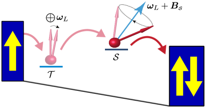
Figure 2: (Color Online). A cartoon model of a two-step transport between the magnetized electrodes. The intermediate states are: a trap, ${\cal T}$, with a long waiting time and no local field, and a site ${\cal S}$, which hosts the field ${\bm{B}}_{\scriptscriptstyle{\cal S}}$. The trap dominates the Hanle response in external field, ${\bm{\omega}}_{L}$, while the site fully controls the value of GMR.

Hanle lineshape in the presence of deep traps. The central notion behind the Hanle effect is that the contribution to nonlocal resistance from a carrier injected at time $t=0$ with spin directed the along the $x$-axis precesses with time as $\cos\omega_{L}t$. The standard Hanle profile emerges upon summation of all these contributions

$$R(\omega_{L})=C\int_{0}^{\infty}dt\cos\left(\omega_{L}t\right)e^{-t/\tau_{s}}P_{L}(t).$$ (6)

Here the weighting factor,

$$P_{L}(t)=\frac{1}{(4\pi Dt)^{1/2}}\exp\left[-\frac{L^{2}}{4Dt}\right],$$ (7)

takes into account that the electron travels to the detector at $x=L$ diffusively, while the factor $\exp\left(-t/\tau_{s}\right)$ describes the spin memory loss with a constant rate $\tau_{s}^{-1}$. Incorporation of traps requires the following modification of Eq. (6). The spin precession takes place both during the time, $t$, spent in course of diffusion, and the time $t_{\scriptscriptstyle tr}$ spent while sitting on the traps. In other words, $\cos\omega_{L}t$ should be modified as follows

$$\cos\omega_{L}t\rightarrow\Big{<}\left<\,\cos\omega_{L}(t+t_{\scriptscriptstyle tr})\right>_{t_{\scriptscriptstyle tr}}\Big{>}_{\{x_{i}\}}.$$ (8)

Here the first averaging is performed over the waiting times spent on traps for fixed coordinates of the traps, while the subscript $\{x_{i}\}$ stands for the positional averaging or, more precisely, for averaging over the positions of the traps that a carrier encounters along its way from injector to detector. Obviously, the order in which the averaging in Eq. (8) is performed is important. This is because the first averaging presumes that the number, $n$, of encountered traps is fixed. For this fixed $n$ the averaging over $t_{\scriptscriptstyle tr}$ reduces to the $n$-fold integral

$$\prod\limits_{j=1}^{n}\int\limits_{0}^{\infty}dt_{j}f_{j}(t_{j})\text{Re}\left\{\exp\left[i\omega_{L}\left(t+\sum\limits_{j=1}^{n}t_{j}\right)\right]\right\},$$ (9)

where $f_{j}(t_{j})$ is the distribution function of the random times, $t_{j}$, spent on $j$-th trap. This time encapsulates the waiting for trapping and waiting for the release. Since the second process is much slower, the distribution is Poissonian

$$f_{j}(t_{j})=\frac{1}{\tau_{j}}\exp{\Bigl{(}-\frac{t_{j}}{\tau_{j}}\Bigr{)}},$$ (10)

where $\tau_{j}$ is the characteristic waiting time for release from the $j$-th trap. With the help of this distribution we readily obtain

$$\langle\cos(\omega_{L}(t+t_{\scriptscriptstyle tr})\rangle_{t_{\scriptscriptstyle tr}}\approx\text{Re}\left\{\exp(i\omega_{L}t)\prod_{j=1}^{n}\frac{1}{1-i\omega_{L}\tau_{j}}\right\}.$$ (11)

As a next crucial step, we take into account that the trap levels are distributed within a wide interval, so that the waiting times, $\tau_{j}$, are widely dispersed. Conventionally, see e.g. Refs. WaitingTimesClassic, , FlatteWaitingTimes1, , their distribution is modeled by a function $p(\tau_{j})$ which falls off as a power law $\sim\tau_{j}^{-\alpha}$ at large $\tau_{j}$ and is flat for small $\tau_{j}$. Such distributions are called heavy-tailed in the literature and are characterized by a divergent mean. For concreteness, we will carry out the calculations for the Lorentzian distribution

$$p(\tau_{j})=\frac{2}{\pi}\frac{\tau_{0}}{\tau_{j}^{2}+\tau_{0}^{2}},$$ (12)

corresponding to $\alpha=2$ and cutoff $\tau_{0}$.

Upon averaging with $p(\tau_{j})$, each factor in the product in the integrand of Eq. (11) assumes the form

$$\left<\frac{1}{1-i\omega_{L}\tau_{j}}\right>_{\tau_{j}}=\frac{1}{1-\omega_{L}^{2}\tau_{0}^{2}}\left(1-\omega_{L}\tau_{0}+i\frac{2}{\pi}\omega_{L}\tau_{0}\ln|\omega_{L}\tau_{0}|\right),$$ (13)

which leads to the closed analytical expression for $\langle\cos(\omega_{L}(t+t_{\scriptscriptstyle tr})\rangle_{t_{\scriptscriptstyle tr}}$

$$\left<\langle\cos(\omega_{L}(t+t_{\scriptscriptstyle tr})\rangle_{t_{\scriptscriptstyle tr}}\right>_{\{x_{i}\}}=\left<\frac{1}{(1+\omega_{L}\tau_{0})^{n}}\left(1+\frac{4\omega_{L}^{2}\tau_{0}^{2}\ln^{2}\omega_{L}\tau_{0}}{\pi^{2}(1-\omega_{L}\tau_{0})^{2}}\right)^{n/2}\cos\left[\omega_{L}t+n\tan^{-1}\frac{2}{\pi}\frac{\omega_{L}\tau_{0}\ln\omega_{L}\tau_{0}}{1-\omega_{L}\tau_{0}}\right]\right>_{\{x_{i}\}}.$$ (14)

Averaging over $x_{i}$ in Eq. (14) must be understood as follows. For a given set of the coordinates of traps different diffusion trajectories can visit different number of traps. It is a delicate issue that, depending on the diffusion time, $t$, in the argument of Eq. (6), the number, $n$, of the visited traps is different. This issue is intimately related to the specifics of a random walk which is accompanied by multiple returns to each site visited previously. Clearly, for unidirectional drift, the number of visited traps is $n={\cal N}L$, where ${\cal N}$ is the density of traps, regardless of the travel time. For a diffusion motion, the dependence of $n$ on ${\cal N}$ is superlinear. Indeed, with traps homogeneously distributed along the carrier path, $n$ is proportional to the time $t$ during which the carrier diffuses. In other words

$$n(t)=\frac{t}{\tau^{\ast}},~{}~{}~{}~{}~{}\tau^{\ast}=\frac{1}{D{\cal N}^{2}}.$$ (15)

The physical meaning of $\tau^{\ast}$ is the diffusion time between the neighboring traps. The true numerical factor in Eq. (15) cannot be specified by such a simple reasoning.

The remaining task is to substitute Eq. (14) with $n$ given by Eq. (15) into Eq. (6) and to perform integration over time. As we will see later, the characteristic width of the Hanle curve in the presence of traps is much smaller than a typical trapping time. This allows us to expand Eq. (14) with respect to a small parameter $\omega_{L}\tau_{0}$. The resulting expression for $R_{H}$ takes a simple form

$$R_{H}(\omega_{L})=\int_{0}^{\infty}dt\;\frac{1}{(4\pi Dt)^{1/2}}\cos\left(\omega_{L}t\left[1+\frac{2\tau_{0}\ln|\omega_{L}\tau_{0}|}{\pi\tau^{*}}\right]\right)\exp\left[-\frac{\omega_{L}\tau_{0}t}{\tau^{*}}-\frac{t}{\tau_{s}}-\frac{L^{2}}{4Dt}\right].$$ (16)

Comparing Eq. (16) to Eq. (6), we find that they have the same analytical structure and can be reduced to each other upon replacement

$$\frac{1}{\tau_{s}} \rightarrow\frac{1}{\tau_{s}}+\frac{\omega_{L}\tau_{0}}{\tau^{*}}=\frac{1}{\tilde{\tau}_{s}},$$ (17)

$${\omega}_{L} \rightarrow\frac{2}{\pi}\omega_{L}\left(\frac{\tau_{0}}{\tau^{*}}\right)\ln\frac{1}{\omega_{L}\tau_{0}}={\tilde{\omega}}_{L}.$$ (18)

While the integral Eq. (16) can be evaluated analytically for arbitrary distance $L$ between the electrodes, the effect of traps on the shape of the Hanle profile is most pronounced in the limit of short channel $L\ll(D\tau_{s})^{1/2}$. In this limit, the bare shape Eq. (6) simplifies to

$$R_{H}(\omega_{L})\propto\frac{\sqrt{\sqrt{1+{\omega}_{L}^{2}{\tau}_{s}^{2}}+1}}{\sqrt{1+{\omega}_{L}^{2}{\tau}_{s}^{2}}},$$ (19)

and depends only on the product $\omega_{L}\tau_{s}$. In the presence of traps, this product should be replaced by

$${\tilde{\omega}}_{L}{\tilde{\tau}}_{s}=\frac{2}{\pi}\ln\left[\frac{1}{\omega_{L}\tau_{0}}\right]\frac{\omega_{L}\tau_{s}}{\omega_{L}\tau_{s}+\frac{\tau^{*}}{\tau_{0}}}.$$ (20)

Two important messages can be inferred from Eq. (20): (i ) the presence of traps leads to the narrowing of the Hanle curve from $\omega_{L}\sim\frac{1}{\tau_{s}}$ to $\omega_{L}\sim\frac{1}{\tau_{s}}\left(\frac{\tau^{*}}{\tau_{0}}\right)$, (ii ) for higher fields the Hanle curve are completely flat. The suppression of the widths is given by the ratio, $\tau^{*}/\tau_{0}$, of the diffusion time between the traps to the trapping time. The dependence of this factor on the density of traps is ${\cal N}^{-2}$, as it follows from Eq. (15). Narrowing of the Hanle curves with ${\cal N}$ is illustrated in Fig. 3. Note that in Eqs. (18), (20) we have already set $\tau^{*}$ to be much less than $\tau_{0}$, so that our result Eq. (20) already assumes that the narrowing of the Hanle curve is substantial.

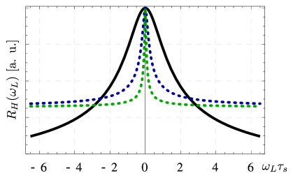
Figure 3: (Color Online). Evolution of the Hanle response, $R_{H}(\omega_{L})$, with the density of traps, ${\cal N}$, measured in the units $(D\tau_{0})^{-1/2}$, is plotted from Eqs. (15), (19), and (20). Three curves correspond to ${\cal N}=0$ (black), ${\cal N}=(2/D\tau_{0})^{1/2}$ (blue), and ${\cal N}=2(2/D\tau_{0})^{1/2}$ (green). Characteristic density, $(D\tau_{0})^{-1/2}$, correspons to one trap per diffusion displacement during the trapping time.

We have also assumed that the characteristic width of the Hanle profile is much smaller than $\tau_{0}^{-1}$. With the width given by $\omega_{L}\sim\frac{1}{\tau_{s}}\left(\frac{\tau^{*}}{\tau_{0}}\right)$, the above condition reduces to $\tau^{*}\ll\tau_{s}$, i.e. the loss of the spin memory on the way between two neighboring traps is small. This condition is implicit for our scenario, since we presumed that the number of visited traps is big.

Discussion. The authors of Refs. NoInjection1, ; NoInjection2, ; NoInjection3, arrived at the conclusion that the Hanle effect in organic spin valves is missing on the basis of the following measurements. The difference, $\Delta{\cal R}$, between the resistances for parallel and antiparallel orientation of magnetizations of electrodes was measured under the conditions when one of the electrodes, CoFeNoInjection2 or CoNoInjection3 , was close to the magnetization reversal. For the orientation of the external magnetic field, ${\bm{\omega}}_{L}$, normal to both magnetizations, measured $\Delta{\cal R}$ did not depend on ${\bm{\omega}}_{L}$. If the conventional Hanle effect was at work, the value $\Delta{\cal R}$ would vanish with ${\bm{\omega}}_{L}$. This is because, the stronger is ${\bm{\omega}}_{L}$, the weaker is the memory of the carrier arriving at the fully magnetized LSMONoInjection1 ; NoInjection2 ; NoInjection3 electrode about its initial spin direction.

Theoretically, the decay of $\Delta{\cal R}$ with ${\bm{\omega}}_{L}$ is described by Eq. (19) and is shown in Fig. 3 with a solid line. In Fig. 3 (dashed lines) we also see that in the presence of traps the Hanle curve does not drop, but stays flat except for a narrow domain of small fields. This plateau behavior would account for the observations of Refs. NoInjection1, ; NoInjection2, ; NoInjection3, . Concerning a narrow peak, if its width is smaller than the resolution in ${\bm{\omega}}_{L}$, it would not show up. This resolution can be set e.g. by the earth’s magnetic field $\sim 0.1$mT.

Here we emphasize that the overall shape of the Hanle curve, in the presence of traps, which is a narrow peak on top of a plateau, is a direct consequence of the broad waiting-time distribution. Without a spread in the waiting times, the traps would simply lead to a homogeneous narrowing of a standard Hanle profile Eq. (19) by a factor $\tau^{*}/\tau_{0}$. This, in turn, would mean that $\Delta{\cal R}$ drops to zero for the applied fields $\omega_{L}\gtrsim\frac{1}{\tau_{s}}\left(\frac{\tau^{*}}{\tau_{0}}\right)$. Thus the unique independence of $\Delta{\cal R}$ of $\omega_{L}$, which is in line with experimental findings, can be traced to the heavy-tailed distribution of the trapping times.

Concluding Remarks:

•  Our main finding that, with spin-preserving traps, the GMR and the Hanle effects become “decoupled” from each other can be elaborated on as follows. The relation $\lambda_{s}=(D\tau_{s})^{1/2}$ no longer holds in the presence of traps. The value $\lambda_{s}$ determined from the thickness dependence of GMR, as in Refs. OrganicValve1', , ValyIsotopes, , does not “know” about the traps. At the same time, the effective ${\tilde{\tau}}_{s}$ defined by Eq. (17), which governs the Hanle profile, does.

•  In the toy model we assumed that the microscopic mechanism of the spin memory loss are the on-site random field. In fact, the origin of $\tau_{s}$ in Eq. (19) for the Hanle profile can be both, random hyperfine fields and spin-orbit interactions.

•  The strong assumption which underlies the decoupling of the GMR and the Hanle effects, adopted in the present manuscript, is that spin-memory is not lost while the carrier sits on the deep trap. This, in turn, requires that the wave function of the trap state does not overlap with hydrogen protons. In experiments Refs. NoInjection1, ; NoInjection2, ; NoInjection3, , the organic layers of spin valves were based on Alq₃ and PTCDI-C4F7 organic molecules. The hydrogen atoms in Alq₃ are attached to approximately $50\%$ of carbon atoms and their locations are well studiedalq3 . It is also accepted that traps play a prominent role in transport through organic layerstraps ; traps1 . However, the spatial positions of the fragments of Alq₃ molecules repsonsible for the trap states are not known. Note also, that in our consideration we have completely neglected the effect of pairs of traps.FlatteTrap

•  Obviously, the flat shape of the Hanle curve in Fig. 3 applies only in a finite field domain. Indeed, in deriving Eqs. (19), (20) we treated the product $\omega_{L}\tau_{0}$, which is the precession angle on a single trap, as a small parameter. It is intuitively clear that for $\omega_{L}\tau_{0}\gg 1$ the Hanle curve should decay. What is surprising, is that this decay is very slow. To capture it analytically, one has to take the $\omega_{L}\tau_{0}\gg 1$ limit of Eq. (14) and use it in Eq. (16) instead of the low-field expansion. The result amounts to replacement $\omega_{L}\tau_{0}$ by $\ln(\omega_{L}\tau_{0})$ in the exponent, and also to the replacement of the argument of cosine by $t/\tau^{*}$. This, in turn, leads to the following modification of the Hanle curve Eq. (19): the product $\omega_{L}\tau_{s}$ gets replaced by $\ln(\omega_{L}\tau_{0})$. We see that $R_{H}(\omega_{L})$ does decay at strong enough fields, but this decay is logarithmical, i.e. very slow.

•  The essence of the explanationYu of missing Hanle effect in organic structures is assumption that the diffusion coefficient in the spin-transport equation is much bigger than the diffusion coefficient of a current carrier. This assumption is attributed to a strong exchange interaction of two carriers of neighboring hopping sites, so that the spin polarization is sensed by the detector much faster than the injected charge actually reaches it. This makes the spin transport robust to the external field. Such a “spin-wave” scenario is similar to the voltage buildup in magnetic insulator due to the flow of spin-wavesSpinSeebeck1 ; SpinSeebeck2 , and seems questionable since the voltage buildup requires conversion of spin current into the charge current, i.e. inverse spin Hall effect.

Acknowledgements. We are grateful to Z. V. Vardeny for reading the manuscript and providing illuminating remarks. We acknowledge interesting discussions of spin transport with V. V. Mkhitaryan. We have also benefited from discussions with C. Boehme, J. M. Lupton, and A. Tiwari concerning different aspects of the Hanle effect. This work was supported by NSF through MRSEC DMR-1121252.

References

- (1) V. Dediu, M. Murgia, F. C. Matacotta, C. Taliani, S. Barbanera, Solid State Commun. 122, 181 (2002).
- (2) Z. H. Xiong, D. Wu, Z. V. Vardeny, and J. Shi, Nature (London) 427, 821 (2004).
- (3) S. Pramanik, S. Bandyopadhyay, K. Garre, and M. Cahay, Phys. Rev. B 74, 235329 (2006).
- (4) S. Pramanik, C.-G. Stefanita, S. Patibandla, S. Bandyopadhyay, K. Garre, N. Harth, and M. Cahay, Nat. Nanotechnol. 2, 216 (2007).
- (5) F. J. Wang, C. G. Yang, Z. V. Vardeny, and X. G. Li, Phys. Rev. B 75, 245324 (2007).
- (6) V. A. Dediu, L. E. Hueso, I. Bergenti, and C. Taliani, Nat. Mater. 8, 850 (2009).
- (7) R. Lin, F. Wang, M. Wohlgenannt, C. He, X. Zhai, Y. Suzuki, Synth. Metals 161, 553 (2011).
- (8) K. M. Alam and S. Pramanik, Phys. Rev. B 83, 245206 (2011).
- (9) X. Lou, C. Adelmann, S. A. Crooker, E. S. Garlid, J. Zhang, S. M. Reddy, S. D. Flexner, C. J. Palmstrøm, and P. A. Crowell, Nat. Phys. 3, 197 (2007).
- (10) L.-T. Chang, W. Han, Y. Zhou, J. Tang, I. A. Fischer, M. Oehme, J. Schulze, R. K. Kawakami, and K. L. Wang, Semicond. Sci. Technol. 28, 015018 (2013).
- (11) S. Majumder, B. Kardasz, G. Kirczenow, A. S. Thorpe, and K. L. Kavanagh, Semicond. Sci. Technol. 28, 035003 (2013).
- (12) A. J. Drew, J. Hoppler, L. Schulz, F. L. Pratt, P. Desai, P. Shakya, T. Kreouzis, W. P. Gillin, A. Suter, N. A. Morley, V. K. Malik, A. Dubroka, K. W. Kim, H. Bouyanfif, F. Bourqui, C. Bernhard, R. Scheuermann, G. J. Nieuwenhuys, T. Prokscha, and E. Morenzoni, Nat. Mater. 8, 109 (2009).
- (13) M. Cinchetti, K. Heimer, J.-P. Wüstenberg, O. Andreyev, M. Bauer, S. Lach, C. Ziegler, Y. Gao, and M. Aeschlimann, Nat. Mater. 8, 115 (2009).
- (14) V. A. Dediu, L. E. Hueso, I. Bergenti, and C. Taliani, Nat. Mater. 8, 850 (2009).
- (15) M. Grünewald, M. Wahler, F. Schumann, M. Michelfeit, C. Gould, R. Schmidt, F. Wurthner, G. Schmidt, and L. Molenkamp, Phys. Rev. B 84, 125208 (2011).
- (16) M. Grünewald, R. Göckeritz, N. Homonnay, F. Würthner, L. W. Molenkamp, and G. Schmidt, Phys. Rev. B 88, 085319 (2013).
- (17) A. Riminucci, M. Prezioso, C. Pernechele, P. Graziosi, I. Bergenti, R. Cecchini, M. Calbucci, M. Solzi, and V. A. Dediu, Appl. Phys. Lett. 102, 092407 (2013).
- (18) S. Watanabe, K. Ando, K. Kang, S. Mooser, Y. Vaynzof, H. Kurebayashi, E. Saitoh, and H. Sirringhaus, Nat. Phys. 10, 308 (2014).
- (19) X. Zhang, S. Mizukami, Q. Ma, T. Kubota, M. Oogane, H. Naganuma, Y. Ando, and T. Miyazaki, Journ. Appl. Phys. 115, 172608 (2014).
- (20) Z. G. Yu, Phys. Rev. Lett. 111, 016601 (2013).
- (21) J. J. H. M. Schoonus, P. G. E. Lumens, W. Wagemans, J. T. Kohlhepp, P. A. Bobbert, H. J. M. Swagten, and B. Koopmans, Phys. Rev. Lett. 103, 146601 (2009).
- (22) R. C. Roundy and M. E. Raikh, Phys. Rev. B 88, 205206 (2013).
- (23) M. Johnson and R. H. Silsbee, Phys. Rev. B 37, 5312 (1988).
- (24) F. J. Jedema, A. T. Filip, and B. J. van Wees, Nature (London) 410, 345 (2001).
- (25) X. Lou, C. Adelmann, S. A. Crooker, E. S. Garlid, J. Zhang, S. M. Reddy, S. D. Flexner, C. J. Palmstrøm, and P. A. Crowell, Nat. Phys. 3, 197 (2007).
- (26) H. Scher and E. W. Montroll, Phys. Rev. B 12, 2455 (1975).
- (27) N. J. Harmon, and M. E. Flatté, Phys. Rev. Lett. 110, 176602 (2013).
- (28) T. D. Nguyen, G. Hukic-Markosian, F. Wang, L. Wojcik, X.-G. Li, E. Ehrenfreund, and Z. V. Vardeny, Nature Mater. 9, 345 (2010).
- (29) M. Brinkmann, G. Gadret, M. Muccini, C. Taliani, N. Masciocchi, and A. Sironi, J. Am. Chem. Soc. 122, 5147 (2000).
- (30) H. T. Nicolai, M. Kuik, G. A. H. Wetzelaer, B. de Boer, C. Campbell, C. Risko, J. L. Brédas, and P. W. M. Blom, Nature Mater. 11, 882 (2012).
- (31) J. Rybicki, R. Lin, F. Wang, M. Wohlgenannt, C. He, T. Sanders, and Y. Suzuki, Phys. Rev. Lett. 109, 076603 (2012).
- (32) N. J. Harmon, and M. E. Flatté, J. Appl. Phys. 116, 043707 (2014).
- (33) K. Uchida, S. Takahashi, K. Harii, J. Ieda, W. Koshibae, K. Ando, S. Maekawa, and E. Saitoh, Nature, 455, 778 (2008).
- (34) G. Siegel, M. C. Prestgard, S. Teng, and A. Tiwari, Scientific Reports 4, 4429 (2013).