Life and death of a hero – Lessons learned from modeling the dwarf spheroidal Hercules: an incorrect orbit?

Abstract

Hercules is a dwarf spheroidal satellite of the Milky Way, found at a distance of $\approx 138$ kpc, and showing evidence of tidal disruption. It is very elongated and exhibits a velocity gradient of $16\pm 3$ km s^-1 kpc^-1. Using this data a possible orbit of Hercules has previously been deduced in the literature. In this study we make use of a novel approach to find a best fit model that follows the published orbit. Instead of using trial and error, we use a systematic approach in order to find a model that fits multiple observables simultaneously. As such, we investigate a much wider parameter range of initial conditions and ensure we have found the best match possible. Using a dark matter free progenitor that undergoes tidal disruption, our best-fit model can simultaneously match the observed luminosity, central surface brightness, effective radius, velocity dispersion, and velocity gradient of Hercules. However, we find it is impossible to reproduce the observed elongation and the position angle of Hercules at the same time in our models. This failure persists even when we vary the duration of the simulation significantly, and consider a more cuspy density distribution for the progenitor. We discuss how this suggests that the published orbit of Hercules is very likely to be incorrect.

1 Introduction

The Milky Way (MW) has many faint galaxies as satellites. This population of galaxies is constituted by a rich variety, such as dwarf spheroidals, a dwarf irregular (Small Magellanic Cloud, SMC), and a dwarf disc galaxy (Large Magellanic Cloud, LMC) (for an overview see e.g. McConnachie, 2012). The dwarf spheroidal galaxies (dSph) are very faint (e.g. Mateo, 1998), show irregular morphologies (e.g. Irwin & Hatzidimitriou, 1995) and velocity dispersions far too high to be explainable by their luminous matter alone (e.g. Walker et al., 2009). Assuming virial equilibrium makes them the most dark matter (DM) dominated objects in the Universe. This fact is in concordance with the $\Lambda$CDM paradigm (e.g. Millennium II simulation of Boylan-Kolchin et al., 2009) that a galaxy like the MW should be surrounded by many hundreds of smaller DM haloes (Via Lactea INCITE simulation of Kuhlen et al., 2008), which possibly host luminous components, i.e. the dSph galaxies.

With the advent of large surveys like the Sloan Digital Sky Survey (SDSS York et al., 2000) many more of these faint and also ultra-faint dSph galaxies are being discovered (e.g. Belokurov et al., 2007, and many more). Again these galaxies show high velocity dispersions (e.g. Simon & Geha, 2007) and some of them show signs of a possible tidal elongation (e.g. Deason et al., 2012).

If these elongations are in fact tidal tails then these objects cannot be currently DM dominated. They either have formed without DM as tidal dwarf galaxies (TDG; Metz et al., 2007, for the disc of satellites theory) or they have lost a great part of their DM halo through tidal stripping while orbiting the MW (e.g. Smith et al., 2012, for the general picture). The only way to lose mass from the luminous component without affecting the DM halo dramatically would be resonant stripping seen in interacting disc galaxies (see D’Onghia et al., 2009, for a study of this mechanism in the case of dwarf disc galaxies) or resonant tidal disruption when a dwarf disc orbits a larger galaxy like the MW (Mayer et al., 2007).

The Hercules dSph galaxy was discovered recently by Belokurov et al. (2007). Its central surface-brightness is $\mu_{0}\approx 27$ mag arcsec^-2. Hercules lies at a distance of $\approx 138$ kpc from the Milky Way (Adén et al., 2009a; Sand et al., 2009), and its luminosity is likely between $2.68\times 10^{4}$ L_⊙ (Sand et al., 2009) and $3.87\times 10^{4}$ L_⊙ (Coleman et al., 2007). Taking the mean from these two values and using a generic mass-to-light (M/L) ratio of $1.0$ amounts to a stellar mass of $\approx 3.3\times 10^{4}$ M_⊙.

Hercules contains no gas and presents no recent star formation (Adén et al., 2011). These authors also study the chemical abundances of [Fe/H], [Ca/H] and a trend in the [Ca/Fe] abundance, which suggests an early rapid chemical enrichment through type II supernovae, followed by a phase of slow star formation dominated by enrichment through type Ia supernovae. A comparison with the isochrones indicates that the red giants in Hercules are older than $10$ Gyr, which could give us some hints about the age of this object.

The elongated structure observed in Hercules by Coleman et al. (2007) using the Large Binocular Telescope (LBT) suggests that it may be in the process of tidal disruption. Adén et al. (2009a, b) determine a line-of-sight velocity dispersion of $\sigma_{\rm los}=3.72\pm 0.91$ km s^-1, and also a radial velocity gradient of $-16\pm 3$ km s^-1 kpc^-1, measured in distance to the semi-minor axis with respect to the right ascension. From this the authors deduce that Hercules has a component of stars showing rotation.

This gradient could also be associated with an effect of tidal distortion caused by the Milky Way instead of rotation. Assuming that Hercules is in tidal disruption, Martin & Jin (2010) proposed an orbit. Using the measured radial velocities of the stars of Hercules and the orientation of the elongation of Hercules, the authors calculate a tangential velocity using energy and angular momentum arguments.

Sand et al. (2009) estimate a projected half-light radius of $r_{\rm h}=230\pm 30$ pc and a projected ellipticity of $\epsilon=0.67\pm 0.03$. Together with the assumptions of Martin & Jin (2010) a de-projected half-light radius and ellipticity of $r_{\rm h,deproj}\approx 1.5$ kpc and $\epsilon_{\rm deproj}\approx 0.95$ are estimated.

The goal of this paper is to test if we can reproduce the observations of the dwarf galaxy Hercules under the assumption that the published orbit is correct and that indeed Hercules is undergoing tidal disruption. In the next section we explain the setup of our simulations followed by the sections describing our results. We end this paper with some conclusions and a discussion of our results.

2 Setup

Dwarf spheroidals are thought to be the oldest galaxies in the universe, forming around re-ionisation (Koposov et al., 2009). In isolation they are not expected to strongly change their structural parameters. This changes when they start to orbit in the tidal field of the MW. As the infall time of Hercules is unknown we will initially fix the simulation time to be $10$ Gyr. Although this choice is rather arbitrary it mimicks the fact that the stars of Hercules are old. However, we also consider a 5 Gyr simulation time later in the paper.

We choose to start our simulations with a ‘DM free’, one-component spherical object - specifically we choose a Plummer sphere. As a result its properties are fully described by only two parameters, e.g total mass and scalelength. This reduces significantly the parameter space we would need to study if we were to include a model with a dark matter halo. Our models often become extended along their orbital trajectory by tidal disruption, resulting in final models that are elliptical in shape. In fact, the process of being tidally extended was implicit in the derivation of the orbit of Hercules that we will assume throughout this paper. However, as we will demonstrate none of our models can match the observed ellipticity of Hercules. Smith et al. (2012); Peñarrubia et al. (2008) demonstrate that a dwarf galaxy’s dark matter halo provides an effective shield, protecting the baryons from tidal stripping until the dark matter halo has been almost entirely removed. As the ellipticity is produced by tidal disruption, the inclusion of a dark matter halo can only reduce the ellipticity further, causing even greater disparacy with the observations (i.e. a dark matter free progenitor will clearly be most effected by tides). Thus our main result - that the failure to match the observed ellipticity suggests that the orbit is not correct - is not reliant on our choice of a dark matter free progenitor. In fact we will also demonstrate that this conclusion is robust - independent on the choice of spherical distribution, and furthermore independent of the assumed infall time as well.

We use the published position of Hercules of RA (J2000) $16^{\rm h}31^{\rm m}02^{\rm s}\pm 14^{\prime\prime}$ and Dec (J2000) $12^{\rm o}47^{\prime}13.83^{\prime\prime}\pm 5^{\prime\prime}$ on the sky as well as the mean out of all distance estimates, i.e. $138\pm 7$ kpc as our initial position. For the velocities we use the published radial velocity of $v_{\rm r,GSR}=144.7\pm 1.2$ km s^-1. Martin & Jin (2010) used the measured velocity gradient and the orientation of Hercules to determine a tangential velocity, using energy and angular momentum arguments. They determine an angle for the tangential velocity of $\theta=78\pm 4^{\rm o}$ and $v_{\rm t}=-16^{+6}_{-22}$ km s^-1. Following their findings we now have the full phase space position of Hercules today. These values transformed into a Cartesian coordinate system are shown in the second column of table 1.

Table 1: Position and velocity of Hercules today and at the start of our simulations. The position today is calculated using the published position in RA and Dec and the mean of the distance estimates of $138$ kpc. The velocities are determined using the published radial velocity and the tangential velocity determined by Martin & Jin (2010). The position and velocity at $-10$ and $-5$ Gyr are calculated using the values from today and performing a test-particle orbit calculation inside an analytic MW potential.

Hercules	observed	calculated	calculated
	values	values	values
t [Gyr]	0	-10	-5
X [kpc]	-88.81	-92.29	58.18
Y [kpc]	-53.06	74.48	24.36
Z [kpc]	82.80	182.13	98.16
$V_{X}$ [km s-1]	-94.95	32.36	-96.98
$V_{Y}$ [km s-1]	-48.10	16.87	-42.75
$V_{Z}$ [km s-1]	99.32	-15.24	-124.71

We now have to assume a suitable potential for the MW, which fits the observations as well as theoretical predictions. Again we follow Martin & Jin (2010) and use a superposition of several analytical potentials to simulate the different structures of the MW.

We use a Miyamoto-Nagai profile (Miyamoto & Nagai, 1975) for the disk, defined by Paczyński (1990):

$$\Phi^{\rm MN}_{\rm disk}\left(R,z\right) = \frac{-GM_{\rm disc}}{\left(R^{2}+\left[a+\left(z^{2}+b^{2}\right)^{1/2}\right]^{2}\right)^{1/2}}$$ (1)

where $R^{2}=x^{2}+y^{2}$, with the parameters $a=3.7$ kpc, $b=0.2$ kpc and $M_{\rm disc}=8.07\times 10^{10}$ M_⊙.

For the bulge we use a Plummer profile (Plummer, 1911) also defined by Paczyński (1990):

$$\Phi^{\rm Plum}_{\rm bulge} = \frac{-GM_{\rm bulge}}{\sqrt{r^{2}+r_{\rm Plum}^{2}}}$$ (2)

with $r_{\rm Plum}=0.277$ kpc and $M_{\rm bulge}=1.12\times 10^{10}$ M_⊙.

For the DM halo potential, we use an adiabatically contracted Navarro-Frenk-White halo (Navarro, Frenk & White, 1997) constrained by Xue et al. (2008):

$$\Phi^{\rm NFW}_{\rm halo}\left(r\right) = -4\pi G\rho_{0}r^{3}_{s}\left[\frac{\ln\left(1+r/r_{s}\right)}{r}-\frac{1}{r_{c}+r_{s}}\right]$$ (3)

with $r_{s}=41.67$ kpc, $r_{c}=r_{vir}=275$ kpc, $M_{\rm NFW}=\frac{4\pi}{3}\rho_{\rm cr}\Omega_{m}\delta_{\rm c}r_{vir}^{3}=10^{12}$ M_⊙ and $\rho_{0}=\rho_{\rm cr}\delta_{\rm c}$.

Using this potential we calculate the position and velocity of Hercules $10$ Gyr backwards in time using a simple test particle integration. The position and velocities at that time are given in the third column of Tab. 1. We use this position and velocities as initial conditions for our simulations.

As explained earlier, we do not simulate any DM component of Hercules. Instead we choose a simple Plummer model to mimic the initial state of Hercules. As shown in Eq. 2, this model is characterised by two parameters only: the initial mass $M_{\rm pl}$ and the initial scale-length, the Plummer radius $R_{\rm pl}$ (we use different symbols here to distinguish from the values for the bulge potential).

Plummer spheres with different initial parameters ($M_{\rm pl},R_{\rm pl}$) are inserted at the calculated position and then simulated forward in time using the particle-mesh code Superbox (Fellhauer et al., 2000).

As opposed to previous similar studies (Fellhauer et al., 2007a; Smith et al., 2013) we choose to investigate a larger parameter space of initial values to assess the general trends and behaviour of our models in a systematic manner, instead of searching for a best matching model by a trial and error approach. We use Plummer masses of $5\times 10^{4}$, $10^{5}$, $1.5\times 10^{5}$, $1.8\times 10^{5}$, $1.9\times 10^{5}$, $2\times 10^{5}$, $5\times 10^{5}$, and $10^{6}$ M_⊙. The Plummer radii we vary to be $10$, $30$, $50$, $60$, $65$, $70$, $75$, $80$, $100$, and $150$ pc. The values chosen are not equally spaced as there are more data points in the parameter space region of interest. In those regions we performed even more simulations, which are not associated with the grid-points mentioned above. In total we perform a suite of 70 simulations.

We repeat part of the experiment using a simulation time of only $5$ Gyr. The initial position and velocities are given in the last column of Tab. 1. For these simulations only a small part of the initial parameter space is used (27 simulations).

Finally, we perform a few simulations using a cuspy Hernquist profile for the initial satellite instead of a Plummer sphere to look for differences in the results. We discuss the results of these simulations in Sect. 4.2.

3 Results

3.1 Parameters of Hercules

In Tab. 2 we show the observational parameters we try to match.

Table 2: Observational properties of Hercules we try to fit with our models: $M_{\rm fin}$ is the final mass (no errors given because of the generic $M/L$-ratio, see main text), $\mu_{0}$ is the central surface-brightness, $r_{\rm h}$ is the projected half light radius, $\sigma_{\rm los}$ is the line-of-sight velocity dispersion, $\Delta v_{\rm r}$ the radial velocity gradient, $\varepsilon$ the ellipticity and $\theta$ the position angle.

Final mass	$M_{\rm fin}$	$3.3\times 10^{4}$ M⊙
Central surface-brightness	$\mu_{0}$	$27.2\pm 0.6$ mag arcsec-2
Projected half-light radius	$r_{\rm h}$	$230\pm 30$ pc
Velocity dispersion	$\sigma_{\rm los}$	$3.72\pm 0.91$ km s-1
Velocity gradient	$\Delta v_{\rm r}$	$-10.2\pm 6$ km s-1 kpc-1
Ellipticity	$\varepsilon$	$0.67\pm 0.03$
Position angle	$\theta$	$-78^{\rm o}\pm~{}4^{\rm o}$

As we are using particles with masses, we convert the mean value of the observational total $V$-band luminosities into a mass using a generic mass-to-light ratio ($M/L$) of unity which gives us a final mass of $3.3\times 10^{4}$ M_⊙ (mean value of the two observationally determined luminosities). An old population like Hercules is more likely to have a stellar mass-to-light ratio of a few. So, e.g. assuming a $M/L=2$ would lead to a final mass of double the value.

To compute the mass of our model, we cannot use the remaining bound mass only, as it is assumed that the object (Hercules) we see is mainly a stream of unbound particles. So we decide to use the mass of all particles which are located in a rectangle of the size of the visible Hercules dwarf (Coleman et al., 2007, their figure 2), i.e. a rectangle spanning $\pm 0.2$ degrees in right ascension and $\pm 0.1$ degrees in declination from the centre of our object.

We use the same generic $M/L$ to convert our surface densities into surface brightnesses to match the observational value. A value of $2$ would make our models approximately $0.6$ mag arcsec^-2 fainter. To obtain the central value, we construct pixel maps with a resolution of $80$ pixels per degree and use the value of the brightest pixel. At the distance of Hercules the size of one pixel is about $30$ pc. So we can be sure to get a good mean value for the central surface brightness, better than relying on any radial fit, which might not be a good description of the actual profile at all. We have to deal with a wide range of possible results. While an almost undestroyed dwarf is well fitted by a Plummer profile, we would lose the information of the faint tails providing the elongation. Simulations leading to tidally more disturbed models would be best fitted by an inner profile of the bound remnant and an outer fitting the strong tidal tails. Finally, totally destroyed models won’t show any strong density enhancements any longer. As there is no global profile which could accommodate all these different outcomes of our simulations and the fitted central surface brightness might be very different depending on the profile used, we decided not to rely on a fit to determine this quantity.

To obtain the effective radius we have no other choice than to rely on a radial fit. We measure the surface brightness, i.e. surface density, in concentric rings around the centre of Hercules, but as seen by an observer projected on the sky and then use the actual distance of our model object to convert degrees into parsec. We fit a Plummer profile (as we start out with an initial Plummer sphere) to the data points and use the Plummer radius from this fit as half-light radius. It can be shown analytically that the Plummer radius contains half of the mass in projection. As we do not want to measure the profile of a remaining dense and bound core, we restrict the fitting routine to values between $0.1$ and $0.5$ degree around the centre of Hercules to ensure we measure the profile of the tidally disturbed envelope. This procedure leads to spurious results for models which are still tightly bound and had only a small mass-loss, as will be explained in the corresponding section below.

Adén et al. (2009a) use the spectra of stars within about $\pm 0.2$ degrees in right ascension and about $\pm 0.1$ degrees in declination from the centre of Hercules to obtain the velocity dispersion. We use all particles in this area to compute the total line-of-sight velocity dispersion of our model.

The measured velocity gradient is based mainly on two stars lying approximately $0.35$ degrees apart from each other. Adén et al. (2009a) calculate from that a velocity gradient of about $-16$ km s^-1  kpc^-1. But the orbit obtained by Martin & Jin (2010) only shows a gradient of $-10.2$ km s^-1 kpc^-1. As this is the gradient the stars would have if they just follow the orbital path and without any peculiar motion we regard the value of Martin & Jin (2010) as an upper limit, which we try to match. To calculate the gradient we calculate the mean radial velocity of all particles located in two thin stripes of right ascension at $\pm 0.2$ degrees from the centre of Hercules and give the difference.

To calculate the ellipticity and the position angle (with respect to the declination axis) we use again the pixel maps with $80$ pixels per degree. These pixel maps are then analysed using the routine Ellipse of IRAF. As position angle and ellipticity vary with radius, we use the values at a radius of $10$ pixels (approximately $0.2$ degrees) to match the observed quantities.

3.2 Technique to obtain a best match model

Having measured each parameter, we then proceed with the following routine to find the best match model:

1. We plot the results as a function of initial mass $M_{\rm pl}$ for all simulations having the same initial Plummer radius in a double logarithmic plot.

2. We see that the data points in the region of interest follow a straight line, i.e. follow a power-law.

3. We fit a straight line to the data points in the double logarithmic space to obtain the power-law.

4. We use the fitted line to calculate the value of initial mass (with its errors) which we need to match the observable for each choice of Plummer radius.

5. We follow the same procedure as (i)–(iv), now plotting the results as a function of the initial Plummer radius for each given initial mass. Then we fit lines to the results in the area of interest and determine the value of the Plummer radius we would need to match the observable.

6. We plot all these pairs of possible matches to the observable in a double logarithmic plot of the initial parameters.

7. We see that those points lie on a straight line, i.e. follow a power-law, as well.

8. We fit a straight line to the data points to obtain the power-law.

9. Finally, we plot all the obtained power-laws and check if all the lines intersect in the same point (i.e. within the same region regarding the errors) of initial parameter space. This is the location for the best fitting model.

3.3 Application of the technique to Hercules

We apply this technique in an attempt to find a best-match model for Hercules. In order to provide a clear example, we describe the procedure used to try to match each of the observed parameters of Hercules individually:

3.3.1 Final mass

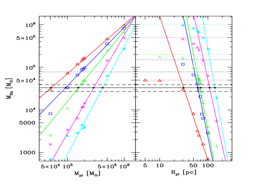
Figure 1: Left panel: Final mass of our object as function of the initial Plummer mass. We show the data points and the fitting lines for Plummer radii of $30$ (red, open triangles), $50$ (blue, open squares), $65$ (green, tri-pointed stars), $80$ (magenta, crosses), and $100$ pc (cyan, filled triangles). Right panel: Final mass as function of the initial Plummer radius. We show data points and fitting lines for initial masses of $5\times 10^{4}$ (red, open triangles), $1.5\times 10^{5}$ (blue, open squares), $2\times 10^{5}$ (green, tri-pointed stars), $5\times 10^{5}$ (magenta, crosses), and $10^{6}$ M_⊙ (cyan, filled triangles). Horizontal solid line denotes the adopted value of the final mass we want to match, dashed lines are the observational errors of this value using the same $M/L$-ratio, and the dashed dotted line is the value we would need to match if we choose a $M/L$ of $2$. Black data points (filled squares) are the matching values calculated by fitting power laws to the data points. In the right panel additional dashed lines are shown in colour denoting the initial masses of the models shown in the same colour code.

Figure 2: Pairs of initial parameters which lead to final models with the correct mass of Hercules.

We measure the final mass of our objects as described in Sec. 3.1. In Fig. 1 we show for parts of our parameter space how our resulting final masses depend on the initial parameters.

The left panel shows the dependency of the final mass on the initial mass as a function of the initial scale-length. We see that for each choice of Plummer radius the final mass drops with smaller initial masses, which is obvious. Furthermore, we see that the final mass drops more rapidly, the larger the initial Plummer radius is. This is also quite obvious as more extended objects are more strongly affected by the tides of the MW.

That the results follow strict power laws is not quite that obvious. As long as we are not in the regime of pure tidal streams, without a central object (lower left corner of the panel) we can easily fit power laws of the form $\log_{10}(M_{\rm fin}[M_{\odot}])=a*\log_{10}(M_{\rm pl}[M_{\odot}])+b$ to the result and are able to calculate, for each initial Plummer radius, which choice of initial Plummer mass would match the required final mass. For the curves shown, we plot the matching values as black squares (omitting the error-bars for clarity).

In the right panel we plot the same data, now showing the dependency of $R_{\rm pl}$ as function of different $M_{\rm pl}$. Again we see that the results follow power laws, except for when we get close to the initial mass. Then we have a turnover of the data points to a much shallower dependency on the left side of each curve. Here we are in the very tightly bound regime (small Plummer radii) and the objects in our simulations have not lost much of their mass.

We again fit power laws of the form $\log_{10}(M_{\rm fin}[M_{\odot}])=a*\log_{10}(R_{\rm pl}[pc])+b$, now to the steep part of the curves only, to obtain the matching values, which are again plotted as black squares in the panel (again omitting the error-bars for clarity).

In Fig. 1 we only show part of the parameter space, because otherwise the figure would be crowded. We determine the fitting power laws over our entire parameter space and show the matching values, obtained in both ways, i.e. as function of $R_{\rm pl}$ and $M_{\rm pl}$ in Fig. 2. In this figure all data points have large error-bars, but only in one direction, depending on if we determined a fitting initial mass for a given fixed initial Plummer radius, then the error-bars are in the mass direction, or if we determined a fitting Plummer radius for a given initial mass, then the error-bars are in the radius direction. The fitting values were determined in logarithmic space and exhibit quite large error-bars, which are symmetric, i.e. have the same length in both directions as we again plot them in a logarithmic plot.

Despite the large error-bars the matching values seem to follow a tight power-law. Therefore, we again fit a simple power law of the form

$$\log_{10}(M_{\rm pl}[M_{\odot}]) = a\log_{10}(R_{\rm pl}[pc])+b$$ (4)

through these fitted, matching values and obtain $a=2.03\pm 0.07$ and $b=1.58\pm 0.12$ which leads to

$$M_{\rm pl} =38^{+12}_{-9}R_{\rm pl}^{2.03\pm 0.07}.$$ (5)

This line in our 2D parameter space of initial conditions gives us all pairs of initial parameters which would fit our adopted final mass of Hercules. Note, that the unsymmetric error of the first value in Eq. 5 (and in the subsections below) solely reflects the transformation of an error determined in logarithmic space into regular space and not any kind of sistematics.

3.3.2 Surface brightness

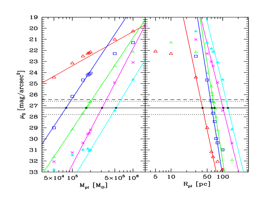
Figure 3: Left panel: Final central surface brightness of our object as function of the initial Plummer mass. We show the data points and the fitting lines for Plummer radii of $30$ (red, open triangles), $50$ (blue, open squares), $65$ (green, tri-pointed stars), $80$ (magenta, crosses), and $100$ pc (cyan, filled triangles). Right panel: Final central surface brightness as function of the initial Plummer radius. We show data points and fitting lines for initial masses of $5\times 10^{4}$ (red, open triangles), $1.5\times 10^{5}$ (blue, open squares), $2\times 10^{5}$ (green, tri-pointed stars), $5\times 10^{5}$ (magenta, crosses), and $10^{6}$ M_⊙ (cyan, filled triangles). The horizontal solid line denotes the observational value we want to match, dashed lines the observational errors and dash-dotted line the value we would need to match if we choose a $M/L$ of $2$, i.e. how much the data points would shift down to lower surface brightnesses. Black data points (filled squares) are the matching values calculated by fitting power laws to the data points.

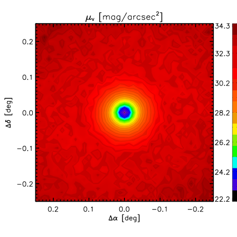
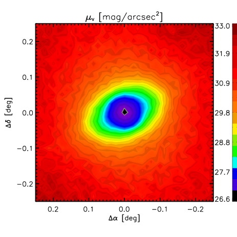
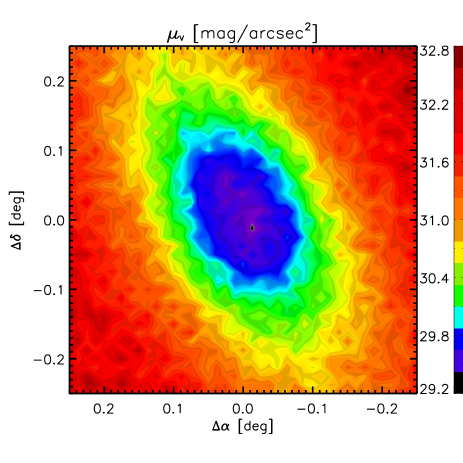
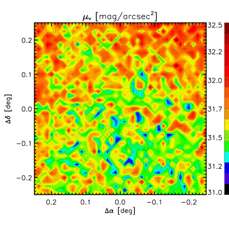
Figure 4: Surface brightness contour plots (resolution 80 pixel per degree) of four of our models with an initial mass of $2.0\times 10^{5}$ M_⊙. Top left panel shows the resulting object, using an initial Plummer radius of $30$ pc, which is in the ‘bound’ regime (see main text for explanation). The model shown in the top right panel has an initial Plummer radius of $65$ pc and is in the ‘tidal regime’. The lower left panel shows the $80$ pc simulation in the transition phase and the lower left panel the $100$ pc simulation which ends up in the ‘stream’ regime. Please note the different colour maps at the side of each panel as we are always using the full 256-colour space to map the brightness differences in all panels separately.

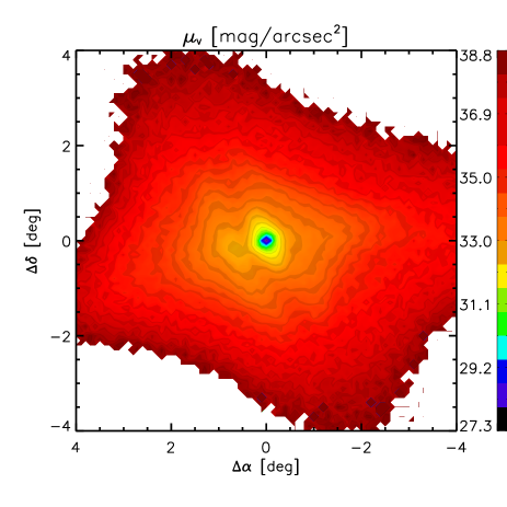
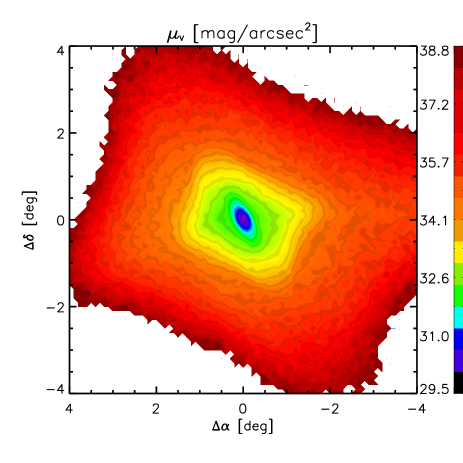
Figure 5: Surface brightness contours for two simulations shown in Fig. 4 showing a larger area of the sky. The strange ‘X-wing’ shape is clearly visible in both simulations. Only the very innermost contours in the left panel are oriented along the orbit. In both cases the intermediate contours are almost perpendicular to the orbit, while the outermost are showing the ‘X’-shape. Black line in both panels denotes the direction to the Galactic Centre.

Figure 6: Pairs of initial parameters which lead to final models with the correct central surface brightness of Hercules.

Now we measure the central surface brightness in all of our models and plot the data in the same way as described in Sect. 3.3.1 in Fig. 3. We use again a generic $M/L=1.0$ to convert our simulation surface densities (solar masses per square parsec) into magnitudes per square arcsecond. In the figure we also show a dashed-dotted line which has an off-set of $0.6$ magnitudes. This represents the downward shift to fainter magnitudes all data points would have if we would have used $M/L=2.0$ instead.

In both panels of Fig. 3 we can detect three regimes of the data points. In the left panel we see that for higher masses the increase in surface brightness flattens off. Here we are in what we refer to as the ‘bound’ regime. In this regime, we still have an almost spherical central object, which is surrounded by a low density of unbound material. The central part of the object is almost unaffected by the mass-loss from the outer parts. The central surface density (brightness) varies slowly with the strength of the mass loss (i.e. the decrease in initial mass).

Except for our simulations with Plummer radii of $30$ pc and below, which always remain in this bound regime (see red (top) line in left panel of Fig. 3 for the $30$ pc data), we see that the data points turn into a steep power law dependency in the so-called ‘tidal’ regime. Here our object is heavily influenced by the tidal field and has lost half of its bound mass or more at the end of the simulation. The galaxy model appears to be elongated and is surrounded by a lot of unbound material. We use the data points in this regime to deduce the fitting initial mass for each Plummer radius (see left panel) and the fitting Plummer radius for each initial mass (see right panel).

Finally, at low masses in the left panel and for large Plummer radii in the right panel we identify a third regime, where again the steep power-law dependency of our results levels off. We refer to this as the ‘stream’ regime. Here we have no or almost no central bound object any longer and the particles of our simulations simply form a stream along the orbit of the former dSph galaxy.

We plot surface brightness pixel maps of our simulations in Fig. 4 to illustrate the different regimes for simulations with an initial mass of $2.0\times 10^{5}$ M_⊙. In the top left panel we see the ‘bound’ regime (initial Plummer radius of $30$ pc). The object has only barely increased in size, it is a small spherical bound object, surrounded by low density extra-tidal material. In the top right panel we see a typical simulation which is in the ‘tidal’ regime at the end of its $10$ Gyr of evolution (initial Plummer radius of $65$ pc). The object is much larger than its initial size and is elongated along the adopted orbit. It is within this regime that we search for a possible progenitor of Hercules.

Before we enter the ‘stream’ regime (lower right panel, initial Plummer radius of $100$ pc), we see a strange flip in orientation of our object. If we show, for example, the result of our simulation with an initial Plummer radius of $80$ pc (lower left panel) we see an object which is elongated almost perpendicular to its orbit. The reason for this strange behaviour is that we are looking at an object which is at the brink of its destruction. A lot of the left-over material is now streaming through the two Lagrange points (pointing directly towards and away from the Galactic Centre, i.e. perpendicular to the orbital path) into the tidal tails. This new material is lost during and shortly after perigalacticon and forming ‘new’ tidal tails, which are not yet aligned with the orbit. With time (i.e. close to apogalacticon) they will ‘flip over’ and align with the old tails (see e.g. Klimentowski et al., 2009, for more details). In between we may see a strange shape, which we dubbed ‘X-wing’ tails. Normally, the ‘old’ tails are denser and are responsible for the visible elongation along the orbital path of the dwarf. At the end of the destruction process the dwarf loses a larger amount of mass, at say the last possible perigalacticon before total destruction and therefore the stars in the not-yet flipped tails might outshine the ‘old’ tails, leading to a flipped orientation of the elongated dwarf.

In all cases if we look at the surface densities in a much larger area and down to brightnesses which are not observable any longer, we always see the ‘X-wing’ shape formed by the unbound stars. In Fig. 5 we show a larger part of the sky ($4\times 4$ degree) for two of our simulations (same as shown in Fig. 4 top right and lower left panel). We see that in the left panel (simulation in the ‘tidal’ regime, without flipped contours) only the very innermost contours (which are also the only observationally visible contours) are aligned with the orbit. Further out the contours are ‘flipped’. The very low density contours at far distances of the remnant show the X-shape. The right panel shows a ‘flipped’ simulation, i.e. also the innermost contours are ‘flipped’ (again the only contours in the observable brightness range) as are the intermediate ones and the outer contours show the X-shape.

In the ‘stream’ regime (shown in the lower right panel of Fig. 4) we finally see a broad low-density stream of material along the projected orbit.

As explained in section 3.3.1 we use the same analysis procedure and fit power-law lines to the data points in the ‘tidal’-regime. This results in matching values of initial mass for each choice of initial Plummer radius and in matching values of initial Plummer radius for each value of initial mass. Again, these solutions have only errors in one dimension, as the other dimension is given. In Fig. 6 we plot all the solutions with their error-bars in the initial parameter space. Again all solutions follow a tight power-law despite the large error-bars. If we fit a power-law of the form of Eq. 4 to the data points we obtain $a=2.608\pm 0.034$ and $b=0.495\pm 0.063$ which translates into the relation:

$$M_{\rm pl} = 3.1^{+0.5}_{-0.4}R_{\rm pl}^{2.608\pm 0.034},$$ (6)

describing the one-dimensional solution space of simulations showing the correct surface brightness at the end of the evolution.

3.3.3 Effective radius

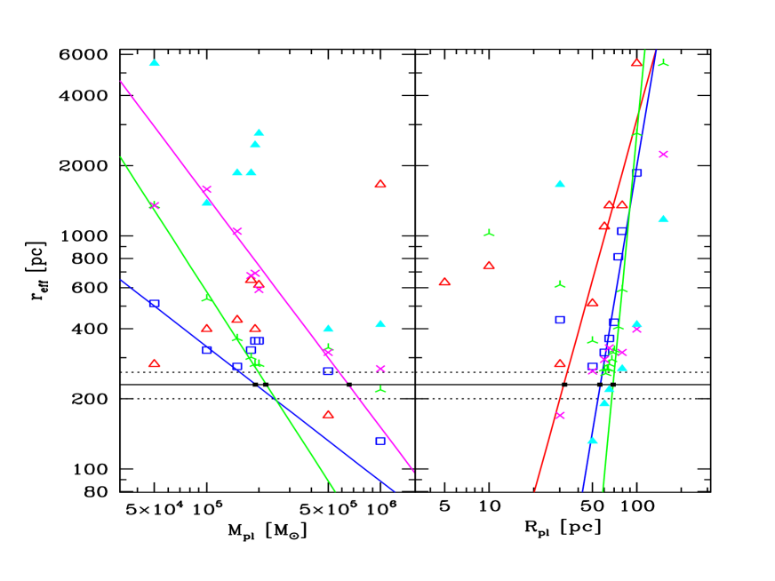
Figure 7: Left panel: Final effective radius of our object as function of the initial Plummer mass. We show the data points and the fitting lines for Plummer radii of $30$ (red, open triangles), $50$ (blue, open squares), $65$ (green, tri-pointed stars), $80$ (magenta, crosses), and $100$ pc (cyan, filled triangles). Right panel: Final effective radius as a function of the initial Plummer radius. We show data points and fitting lines for initial masses of $5\times 10^{4}$ (red, open triangles), $1.5\times 10^{5}$ (blue, open squares), $2\times 10^{5}$ (green, tri-pointed stars), $5\times 10^{5}$ (magenta, crosses), and $10^{6}$ M_⊙ (cyan, filled triangles). The horizontal solid line denotes the observational value we want to match, dotted lines the observational errors. Black data points (filled squares) are the matching values calculated by fitting power laws to the data points.

Figure 8: Pairs of initial parameters which lead to final models with the correct projected effective radius of Hercules.

The analysis of the results for the effective radius shown in Fig. 7 is a bit more complicated. As described above we omit the very central $0.1$ degree, which might still host a bound core, from the fitting routine. We only fit out to $0.5$ degree as this is the region of interest, in which the visible part (i.e. the part with measurable surface brightnesses) of Hercules is located. Furthermore, we fit the data with concentric circles and not with ellipses.

This procedure leads to strange results in some parts of the parameter space. If we are in the ‘bound’ regime, we completely neglect the bound object and only fit a profile to the low-density tidal material. The values obtained are in the regime of up to several hundred parsecs but do not follow a strict power-law. As a trend we can say that as we approach the tidal regime the effective radius becomes smaller. This regime is shown in the right part of the left panel and the left part of the right panel in Fig. 7. This regime is followed by the ‘tidal’ regime, in which we again are able to fit steep power-laws to our results and where the results reflect the effective radius of our resulting elongated and inflated objects. Finally, in the ‘stream’ regime we have almost constant density all along the stream. The ‘fitted’ effective radius on the order of more than one kiloparsec reflects now the transversal extension of the tidal stream and not a scale-radius of any kind.

We are not able to fit power-laws to the extreme parts of our parameter space. For low Plummer radii or very high initial masses we are completely in the bound regime and for large initial radii or very low initial masses we are completely in the ‘stream’ regime. For those values of initial parameters which fall into the ‘tidal regime’ we are able to obtain power-law fits. We show the resulting matching results in Fig. 8.

Again the results seem to follow a power-law in initial conditions parameter space much tighter than the error-bars suggest, but not as tight as the final mass or the surface brightness. The fitting values of Eq. 4 are $a=1.837\pm 0.080$ and $b=1.96\pm 0.14$, which translates to a relation of

$$M_{\rm pl} = 91^{+34}_{-25}R_{\rm pl}^{1.837\pm 0.080}.$$ (7)

3.3.4 Velocity dispersion

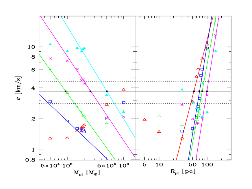
Figure 9: Left panel: Final total velocity dispersion of our object as a function of the initial Plummer mass. We show the data points and the fitting lines for Plummer radii of $30$ (red, open triangles), $50$ (blue, open squares), $65$ (green, tri-pointed stars), $80$ (magenta, crosses), and $100$ pc (cyan, filled triangles). Right panel: Final total velocity dispersion as a function of the initial Plummer radius. We show data points and fitting lines for initial masses of $5\times 10^{4}$ (red, open triangles), $1.5\times 10^{5}$ (blue, open squares), $2\times 10^{5}$ (green, tri-pointed stars), $5\times 10^{5}$ (magenta, crosses), and $10^{6}$ M_⊙ (cyan, filled tri-angles). The horizontal solid line denotes the observational value we want to match, dotted lines the observational errors. Black data points (filled squares) are the matching values calculated by fitting power laws to the data points.

Figure 10: Pairs of initial parameters which lead to final models with the correct total line-of-sight velocity dispersion of Hercules.

We now repeat the same procedure with the overall velocity dispersion. In Fig. 9 we can clearly distinguish two regimes in the results showing a ‘U’-shaped dependency. At high masses in the left panel and small Plummer radii in the right we are in the ‘bound’ regime and the velocity dispersion, even though measured over all particles within the region described above, is mainly due to the bound particles and is related with the bound mass and the Plummer radius according to the virial theorem:

$$\sigma^{2} \sim \frac{\rm Mass}{\rm scale\ radius}.$$ (8)

As the mass-loss in this regime is low, we still see almost the same dependency of the final velocity dispersion on the initial values.

The second solution we find in the ‘tidal’ regime, where the measured velocity dispersion rises quickly with smaller initial masses (left panel) and larger Plummer radii (right panel).

Both regimes may lead to possible solutions but we only take the solutions from the ‘tidal’ regime into account.

The third regime (‘stream’) is visible in the left panel with the results for initial Plummer radii of $100$ pc. At some point we have a saturation of measured velocity dispersion because of the finite extension the stream can have.

Again we fit power-laws to the results in the ‘tidal’ regime and calculate the matching values of initial parameters which result in the correct velocity dispersion. These values with their error-bars are shown in Fig. 10.

The fitting line shown in Fig. 10 has values of $a=3.87\pm 0.10$ and $b=-2.00\pm 0.19$ leading to

$$M_{\rm pl} = 0.01^{+0.02}_{-0.003}R_{\rm pl}^{3.87\pm 0.01}.$$ (9)

3.3.5 Velocity gradient

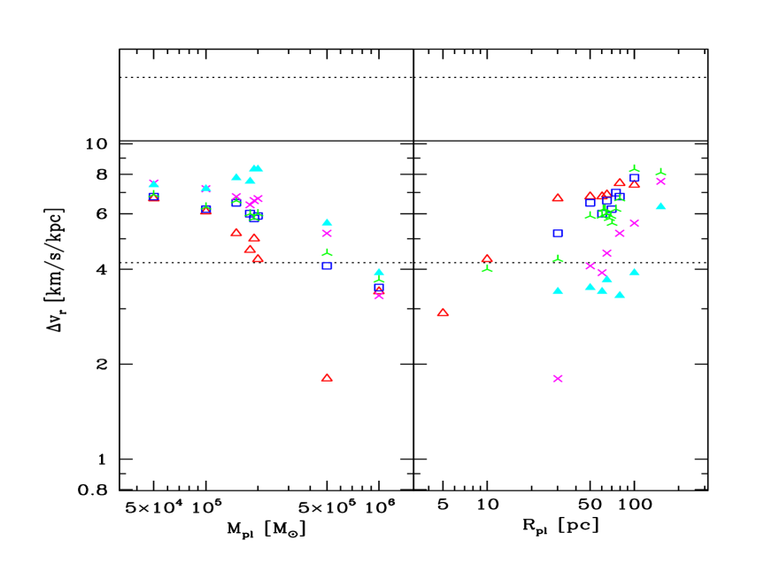
Figure 11: Left panel: Final velocity gradient of our object as a function of the initial Plummer mass. We show the data points for Plummer radii of $30$ (red, open triangles), $50$ (blue, open squares), $65$ (green, tri-pointed stars), $80$ (magenta, crosses), and $100$ pc (cyan, filled triangles). Right panel: Final velocity gradient as a function of the initial Plummer radius. We show data points for initial masses of $5\times 10^{4}$ (red, open triangles), $1.5\times 10^{5}$ (blue, open squares), $2\times 10^{5}$ (green, tri-pointed stars), $5\times 10^{5}$ (magenta, crosses), and $10^{6}$ M_⊙ (cyan, filled triangles). Horizontal solid line denotes the value we want to match based on the assumed orbit, dotted lines the one-sigma deviation of this value.

In Fig. 11 we see the results of our simulations regarding the final velocity gradient measured as described above. We see immediately that the results are not easily fitted with power-laws and also it is impossible to distinguish the three regimes. We see a general trend to smaller gradients if we tend to the ‘bound’ regime, i.e. to larger masses and smaller Plummer radii. None of our simulations fits the velocity gradient adopted by Martin & Jin (2010) but a lot of simulations reach this value within the lower one-sigma error shown. The reason for our small values are two-fold: near-field tidal tails do not need to align with the orbit completely. They may even be perpendicular as seen in the lower left panel of Fig. 4. So the mean radial velocities measured may not have the exact radial velocity a particle, following exactly the adopted orbit for Hercules, would have at this point. Furthermore, we are not dealing with one particle but with an extended tidal tail, where particles are on similar but not on identical orbits and have peculiar motions similar to epicycles as well. So, if we calculate a mean radial velocity at two given points, we will always get a superposition of these two effects and values which are somewhat below the orbital radial velocity difference.

As a result we note that we match the adopted velocity gradient of the orbit to within the one-sigma error for all simulations with masses below $5.0\times 10^{5}$ M_⊙ and for Plummer radii larger than $50$ pc.

3.3.6 Ellipticity and position angle

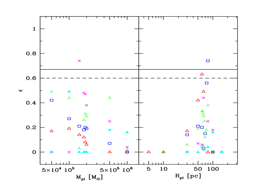
Figure 12: Left panel: Final ellipticity of our object as a function of the initial Plummer mass. We show the data points for Plummer radii of $30$ (red, open triangles), $50$ (blue, open squares), $65$ (green, tri-pointed stars), $80$ (magenta, crosses), and $100$ pc (cyan, filled triangles). Right panel: Ellipticity as a function of the initial Plummer radius. We show data points for initial masses of $5\times 10^{4}$ (red, open triangles), $1.5\times 10^{5}$ (blue, open squares), $2\times 10^{5}$ (green, tri-pointed stars), $5\times 10^{5}$ (magenta, crosses), and $10^{6}$ M_⊙ (cyan, filled triangles). Horizontal solid line denotes the observational value we want to match, dotted lines the observational errors.

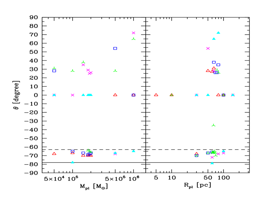
Figure 13: Left panel: Final position angle of our object as function of the initial Plummer mass. We show the data points for Plummer radii of $30$ (red, open triangles), $50$ (blue, open squares), $65$ (green, tri-pointed stars), $80$ (magenta, crosses), and $100$ pc (cyan, filled triangles). Right panel: Final position angle as a function of the initial Plummer radius. We show data points for initial masses of $5\times 10^{4}$ (red, open triangles), $1.5\times 10^{5}$ (blue, open squares), $2\times 10^{5}$ (green, tri-pointed stars), $5\times 10^{5}$ (magenta, crosses), and $10^{6}$ M_⊙ (cyan, filled triangles). Horizontal solid line denotes the observational value we want to match, dashed line the observational error.

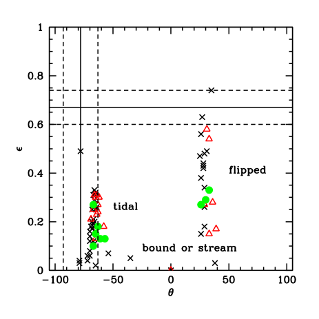
Figure 14: Ellipticity ($\epsilon$) vs. position angle ($\theta$) for all our simulations. Crosses are Plummer spheres with $10$ Gyr of orbital time, triangles (red) are Plummer spheres with $5$ Gyr of orbital time and circles (green) are Hernquist models with $10$ Gyr of orbital time. We clearly see that the results are grouped according to the different regimes (labels).

In Fig 12 we plot the ellipticity of our final object as a function of the initial mass (left panel) and the Plummer radius (right panel).

What we see is that none of our models can reach the correct strong elongation of $\epsilon=0.68$ as observed. The only simulations which show elongations as pronounced as the real Hercules are simulations in the transition regime between ‘tidal’ and ‘stream’, which show a perpendicular orientation of the visible contours (the ‘flipped-tails’ regime). An example of this can be seen in the lower right panel of Fig. 4. We can clearly see the effect of the ‘flipping tails’ (‘X-wing’-effect), which alter the shape of our final object. Therefore in order to reach the observed values of ellipticity, we find we must forfeit the position angle.

Fig. 4 visually demonstrates why this is the case. First we are in the ‘bound’ regime and our object is still spherical, i.e. in this regime the position angle is not defined and set equal to zero. Then we are entering the ‘tidal’ regime, where the position angle is similar to the observed value. This changes dramatically when we enter the transition regime between ‘tidal’ and ‘stream’. There, the position angle has positive values and is almost perpendicular to the observed value. Finally, we enter the ‘stream’ regime where we define the elongation of the model as zero.

For completeness we show the dependency of the position angle on the initial mass and the Plummer radius in Fig. 13. We do not see clear trends in this figure but we can see that we have three regions filled with values and only one of these regions gives values close to the observed value. However, all of the points in this region fail to match the ellipticity of Hercules. This is demonstrated in Fig. 14. Here we plot ellipticity vs. the position angle and clearly see the different regimes of Fig. 4. While we have a completely bound model we have spherical contours so the ellipticity is zero and the position angle is not defined (plotted as zero here as well). Then we enter the ‘tidal’ regime, where we see elongated objects, which have the correct position angle (at least within the errors) but our simulations never reach the strong ellipticity measured for Hercules. Then the simulations change into the ‘flipped’ regime, where the contours of the near field tails are oriented almost perpendicular to the orbit. Only in this regime are we able to match the ellipticity of Hercules, but only at the expense of matching the position angle. Finally in the stream regime we do not have an object and therefore neither position angle nor ellipticity are defined (both set to zero). Fig. 14 demonstrates that, while it is possible to match either the ellipticity or position angle, we fail to match the two parameters simultaneously (see cross symbols, other symbols are discussed in the following section).

4 Best fit model

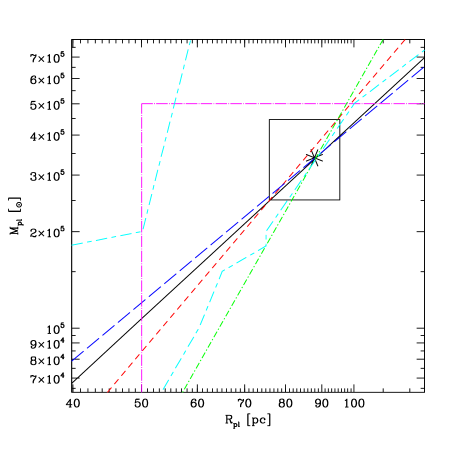
Figure 15: Fitting lines in initial condition space. The black, solid line shows the results matching the final mass, red, short dashed line the results matching the central surface brightness, blue, long dashed line shows results which match the effective radius of Hercules and finally the green, dot-short dashed line shows matching solutions for the velocity dispersion. The magenta dot-long dashed line divides the upper left region which does not match the velocity gradient from the lower right, where our simulations match the gradient within the errors. The two cyan diagonal short dashed-long dashed lines separate the region, where we match the position angle, from the bound region (top left) and the stream region (lower right). Only in between the two lines can we match the position angle of Hercules within the errors. The black square marks the area in which we expect to find a suitable initial model for Hercules. The black star denotes our best-fit model.

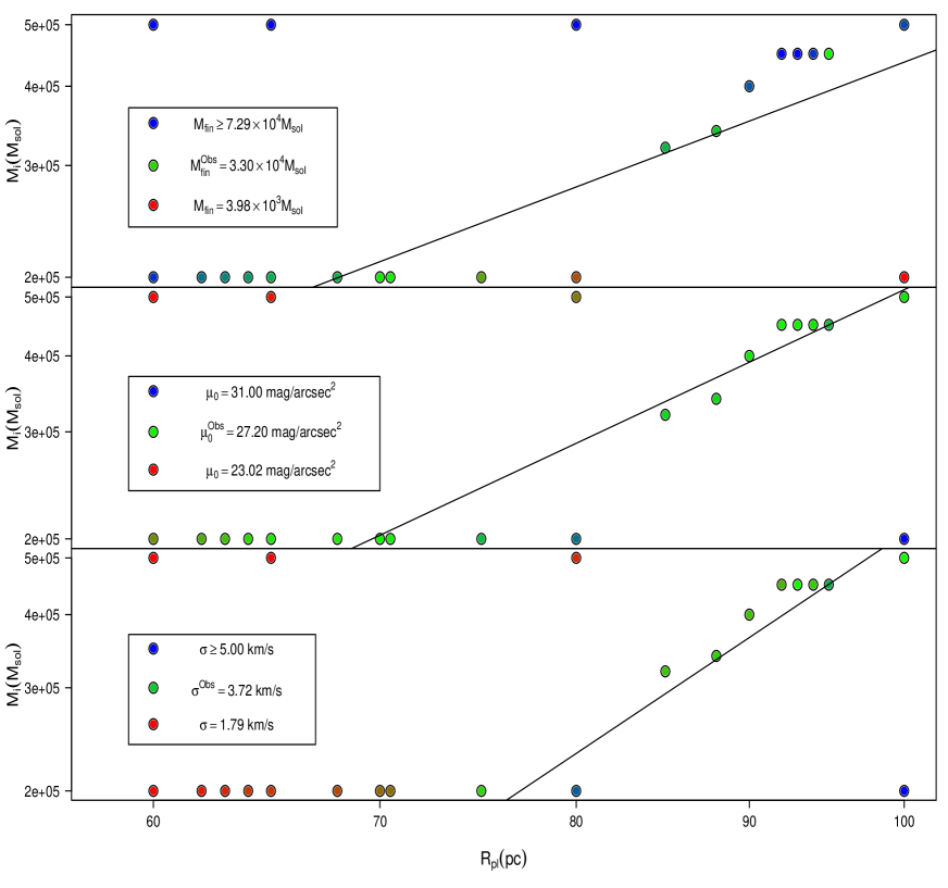
Figure 16: Plots of inital mass-initial scalelength parameter space. Symbol colour relates to final mass (upper panel), central surface brightness (middle panel), and velocity dispersion (lower panel) as indicated by the key. In each key, the middle row is the observed value for Hercules. Black lines join points that should produce the observed value, if our fitting technique is successful. In practice, simulation points that lie near the black line are always close to the observed value, and with increasing distance from the line, the simulation values differ increasingly from the observed value. This is a strong indication that our power-law fitting technique is very effective, and that the fitting technique can successfully be used to predict the outcome of the simulations.

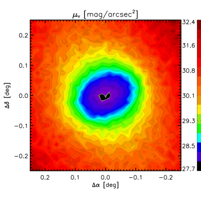
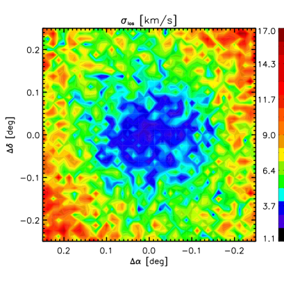
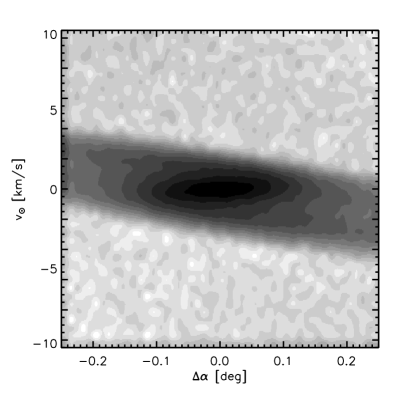
Figure 17: ‘Best match model’. Top: Contour map of the surface brightness of our model converting the mass of our particles using a pixel resolution of $80$ pixel per degree. Middle: Contours of the two-dimensional distribution of line-of-sight velocity dispersions, using the same pixel resolution. Bottom: Density grey-scales of particles in the right ascension – relative radial velocity space.

Having attempted to fit each observational parameters separately, we now attempt to combine the results to produce a best fit model. For this reason we plot all the relations from Eqs. 5, 6, 7, and 9 as well as the boundaries for correct solutions regarding position angle and velocity gradient in one single figure, Fig. 15.

We see that all fitting lines intersect in more or less the same area of the graph (marked with a black square). The differences in the intersection points are all well within the possible errors of the observational data. This area is located in the region where we also match the velocity gradient within its errors and about half of this area (but with all intersecting points above the division line) falls into the region where we expect to get the correct position angle. The correct solution should be found having an initial Plummer radius of $76$ to $96$ pc and an initial mass ranging between $2.5\times 10^{5}$ and $4.4\times 10^{5}$ M_⊙ (keeping the $M/L$-ratio fixed at unity).

We note that the region where the lines are intersecting lies on the boundary between matching the position angle, and the stream region where the models flip their position angle through almost a right-angle (as marked by the lower-right cyan line). Thus the solution space is always on the brink of flipping the position angle, i.e. the region of the correct solution is a solution in which Hercules is already almost destroyed and might not survive for much longer.

We present a best fitting model with the initial parameters of $M_{\rm pl}=3.4\times 10^{5}$ M_⊙ and $R_{\rm pl}=88$ pc. The final mass of this object, measured in the region described above, is $4.56\times 10^{4}$ M_⊙, which is somewhat higher than the mass we try to match with our generic $M/L$-ratio. The central surface brightness of this object is $27.6$ mag arcsec^-2. Therefore, the model fits the central surface brightness within the observational errors. A two-dimensional contour plot of our object is shown in the top panel of Fig. 17. The contours are based on a pixel-map with a resolution of $80$ pixels per degree. We also see that the contours show an object which, in the inner parts is still slightly elongated almost along the orbit, while the outer, fainter parts have already flipped to the perpendicular direction – it is an object at the brink of destruction, having lost about $90$ per cent of its initial mass. Using the same procedure as for our other models we arrive at a position angle of only $-63$ degrees and a small ellipticity of $0.19$.

If we fit a Plummer profile to the surface brightness data calculated in concentric rings around the centre of the object we get a Plummer radius of $0.\!^{\rm o}155\pm 0.\!^{\rm o}007$. At the distance of Hercules this translates into a half-light radius of $186\pm 10$ pc. This is a rather small value but within $2\sigma$ of the observed value.

To demonstrate that our fitting method is effective we perform some additional simulations with initial parameters which differ from the best fit model. In Fig. 16 we demonstrate how these choices of initial parameters result in differing final mass (upper panel), central surface brightness (middle panel) and velocity dispersion (lower panel). Using our fitting procedure, we can predict sets of initial mass/initial scalelength that should reproduce the observed value. These are shown in each panel as a curve. The colour of the symbol shows the actual value measured from the simulation - see legend (the middle row of the legend is the observed value, and is superscripted by ‘Obs’ to indicate this). In all three panels it can be seen that the values measured from the simulation for points near the curve agree very well with the observed value. Furthermore, with increasing distance from the curve, the measured simulation values increasingly differ from the observed values. This is strong confirmation that our fitting method is effective, and that the results of the fitting can truly be used to predict the outcome of the simulation.

In the middle panel of Fig. 17 we show the contours of the line-of-sight velocity dispersion. To achieve this we calculate the velocity dispersion in each pixel of our 2D figure. We are able to do this, as we have more particles in this figure than Hercules would have stars, as the particles of our simulation represent equal-mass phase-space elements and not single stars. We see that in the central region we have a very low velocity dispersion of about $1.5$ to $4.0$ km s^-1. In this region resides the remaining bound body of our object. Even though this velocity dispersion is low compared to the hot regions surrounding that area, it is a very inflated value. A bound object with the mass stated above and a half-light radius of $186\pm 10$ pc would have a dispersion of about $0.6$ km $s^{-1}$, i.e. the velocity dispersion is governed by unbound stars and their different streaming motions in front, within and behind the object (as seen by us). If we compute an overall velocity dispersion as explained at the beginning of this section we get a value of $3.14$ km s^-1, which is in excellent agreement with the observations.

In the bottom panel of Fig. 17 we show densities in the right ascension - radial velocity difference space. The black area in the middle shows the remaining bound object, which shows no velocity gradient, as expected. But around this area we see the streaming motion of the orbit very clearly as a dark grey area. A parallel line through the middle of this area would lead to a velocity gradient of about $-8$ km s^-1 degree^-1. Using the calculation we describe at the beginning of this section, we still obtain a value of $-5.7$ km s^-1 kpc^-1, which is within the errors stated by Martin & Jin (2010).

In summary, our best-fit model can well match the observed values of the luminosity, central surface brightness, effective radius, velocity dispersion and velocity gradient. This demonstrates that the technique for finding a best-match model, as described in Sec. 3.2, is effective at providing the means to simultaneously match multiple properties in a systematic manner. However, despite this success, the technique was unable to simultaneously match the position angle and ellipticity. It is not impossible that one cause of this failure might be that the orbit we have assumed is not that of the real Hercules. However, to support such a hypothesis, we must first demonstrate that the ellipticity-position angle failure continues to occur if we significantly change the duration of the simulation, or if we replace our cored progenitor model with a more cuspy profile.

4.1 Infall 5 Gyr ago

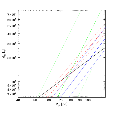
Figure 18: Lines of matching initial models for an orbital time of $5$ Gyr. Color and line-style code as in Fig. 15. Additionally we plot the lines if we shift the power-laws by one sigma in their zero-point. We see that again we find a region where all lines intersect. Here we expect to find a model that matches these particular observables simultaneously.

The true infall time of Hercules into the Milky Way is rather uncertain. So far we have only considered an infall 10 Gyr ago. By considering a more recent infall time of 5 Gyr, we can test if our technique for finding a best match model is robust to varying the duration of the simulation. It is not suprising that the initial parameters of our new best match model will be different than in the 10 Gyr case - in order to match today’s properties of Hercules, the new model must tidally evolve in half the time period. It also allows us to see, if the ellipticity-position angle failure that our best fit model suffers continues when we change the mass loss rate quite considerably.

We perform 27 simulations starting at $t=-5$ Gyr. We repeat the same technique as described previously but with the new simulations. First we derive power-laws of matching initial conditions for the mass:

$$M_{\rm pl} = 95^{+12}_{-11}\cdot R_{\rm pl}^{1.64\pm 0.03},$$ (10)

for the central surface brightness:

$$M_{\rm pl} = 1.31^{+0.21}_{-0.19}\cdot R_{\rm pl}^{2.65\pm 0.04},$$ (11)

the effective radius:

$$M_{\rm pl} = 0.28^{+0.10}_{-0.08}\cdot R_{\rm pl}^{2.91\pm 0.07},$$ (12)

and the velocity dispersion:

$$M_{\rm pl} = 0.61^{+1.32}_{-0.42}10^{-3}\cdot R_{\rm pl}^{4.4\pm 0.3}.$$ (13)

The errors on these fitting lines are quite large as they are based on much less simulations than our main study. Especially, the zero-points of the power-laws are quite ill determined. For this reason we plot in Fig. 18 the fitting lines plus the lines we would obtain if we add or subtract one-sigma in the zero-point.

Then we combine the power laws to find the best-fit model as shown in Fig. 18. We find we are able to find a suitable match, despite the large change in simulation time. However, this time we match only four of the main parameters – namely final mass, central surface brightness, effective radius, and velocity dispersion.

As in the main study we see that all four lines intersect (within their errors) in the same region of the diagram. We, therefore, infer that should the orbital time of Hercules have been only $5$ Gyr we would have to search the correct matching model in a region where its initial parameters are about $R_{\rm pl}\approx 70-80$ pc and $M_{\rm pl}\approx 1.0-1.5\cdot 10^{5}$ M_⊙.

Comparing this with our previous findings shows that we do not need to change the initial scale-length dramatically but we have to search at much lower initial masses (factor $2-4$). By having a lower mass, the model is much more easily destroyed by the tides of the MW, and therefore reaches the same point of destruction we want to observe in a much shorter orbital time.

Unlike in the best-fit model, we cannot match the velocity gradient. It is consistently weaker than in the 10 Gyr duration simulations (although still within the published errors). The position angle and ellipticity show the same behaviour as seen in the $10$ Gyr simulations: with the shorter simulation time we still cannot match the position angle and the ellipticity at the same time. Simulations with the correct ellipticity show the ‘flipped’ orientation and vice versa (e.g. see red triangles in Fig. 14).

4.2 Hernquist models

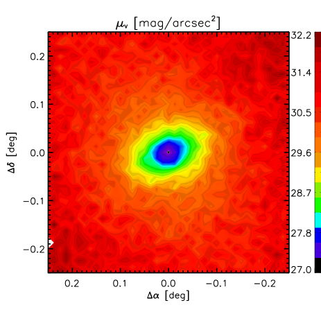
Figure 19: Contour plot of the surface brightness of the best-match Hernquist model – as in the upper panel of Fig. 17 except here for the Hernquist model.

We furthermore tried to match the observables using a cuspy initial model. For a cuspy model, we used Hernquist spheres instead of Plummer models. We use an orbital time of $10$ Gyr to compare them with our main results.

By trial and error, we vary the initial mass and initial Hernquist scalelength, to find a model that closely matches the observed central surface brightness and luminosity of Hercules. Our ‘best-match’ Hernquist model is shown in Fig. 19. This model has a similar final appearance to the best fit Plummer model, although its surface brightness falls off more quickly (e.g. compare with the upper panel of Fig. 17). The best-match Hernquist model has a final mass M${}_{\rm{fin}}=2.9\times 10^{4}~{}$M_⊙, and central surface brightness $\mu_{0}=27.0$ mag arcsec^-2 – each within one-sigma of the observed values.

Furthermore, the velocity gradient is also a reasonable match ($\Delta v_{\rm{r}}=-6.9$ km s^-1 kpc^-1). However, the velocity dispersion $\sigma_{\rm{los}}=7.4$ km s^-1 – over a factor of two too high!. But, looking at the actual distribution of the velocities we see that in the Hernquist models these high dispersions are caused by a few stars with large differences in velocities (in contrary to the Plummer models). If we adopt a clipping function for those velocity tails we obtain a distribution with a FWHM (full width half maximum) of about $3$ km s^-1, i.e. a dispersion which matches the observed one.

The initial mass and scalelength of our best-match Hernquist model is M${}_{\rm{init}}=8.0\times 10^{5}$ M_⊙, and R${}_{\rm{hern}}=0.175$ kpc respectively. Thus, the progenitor Hernquist model is over a factor of two more massive than the progenitor Plummer model. Therefore in order to match the final observed mass, the Hernquist model must lose more than a factor of two more mass than the Plummer model, and this could explain the enhanced velocity dispersion – the Hernquist model is closer to being completely disrupted.

The green circular symbols in Fig. 14 are the results of the various Hernquist models we conducted in the course of finding our best-fit model. Our best-match Hernquist model is the symbol with position angle $\theta=-67^{\circ}$, and an ellipticity $\epsilon=0.27$. Clearly the more cuspy Hernquist models suffer the same fate as the more cored Plummer models – a failure to match the observed ellipticity unless the model is so unbound that it has flipped in position angle. Indeed the low surface brightness, outer contours surrounding our best-match Hernquist model show the same flipped shape as was seen in the best fit Plummer model (e.g. again, compare Fig. 19 with the upper panel of Fig. 17).

In summary, we find that the problem of simultaneously matching the positional angle and ellipticity (e.g. see Fig. 14) is robust to significant changes in the infall time (we change it by a factor of 2), and also to varying the cuspiness of the initial progenitor model. We also see flipped outer-most contours, tracing the unbound stars, in all three best match models (10 Gyr, 5 Gyr, and the Hernquist model). We believe that the flipping of the unbound streams is actually a property of the orbit on which we assume the models follow. If so, this indicates it may be impossible to solve the ellipticity-position angle problem, assuming an initially spherical progenitor that is tidally stripped while moving along the published orbit. We elaborate on the possibility that the orbit is incorrect in the following section.

5 Discussion and Conclusions

We have used a new method to find a suitable model to try to reproduce the observables of the dwarf galaxy Hercules. Instead of trial and error around a possible solution, we made use of a wide parameter space of initial conditions and analysed the general behaviour of every observable as a function of the initial parameters to assess their power-law dependencies in the region of interest. We have shown that we find a relatively small region (smaller than the observational errors) in initial parameter space, where we match several of the observables simultaneously.

We have shown that for the given orbit, the new technique is successful in finding a best-match model for Hercules. We emphasise that the orbit we consider is based on the most probable orbit given in Martin & Jin (2010), and we do not consider possible alternative orbits within the error bounds of the orbital parameters. We also do not take into account that the orbit may have been different in the past (e.g. got changed by a close encounter with another dwarf satellite halo). In our case, Hercules has an initial mass of $3.4\times 10^{5}$ M_⊙ and an initial scale-length of $88$ pc to match the observables today. These values will only change slightly if the orbit turns out to be slightly different (see e.g. the change in initial mass in the models of Fellhauer et al., 2007b) or the orbiting time is only slightly different. We find that, unsuprisingly, shortening the orbital time causes a change in the initial mass and scalelength required to match the luminosity of Hercules. In our case halving the orbital time led to an initial model with a factor 2-3 times lower initial mass, and a slightly smaller scalelength ($\sim 80$ pc).

The best-match model is successful in matching a large number of the observed parameters of Hercules, including luminosity, central surface brightness, effective radius, velocity dispersion, and velocity gradient. This clearly demonstrates the power of the new systematic technique used to find the best-match model. However, despite the thoroughness of the technique, we find it impossible to match the observed ellipticity and position-angle simultaneously in any of our models.

All models on the published orbit show a similar behaviour. While a bound core remains after 10 Gyr, the position angle is close to the observed value, but the core is too round resulting in an ellipticity which is much lower than the observed value. However, models that are slightly more tidally disrupted after 10 Gyr can match the observed ellipticity, but in the process their position angle flips to almost perpendicular to the observed value. This behaviour seems to be an inherent property of the orbit of the galaxy. In fact the ellipticity-position angle problem persists, assuming the published orbit, even when we consider an infall time half as long, and even when we exchange the progenitor model for a much more cuspy density profile. We note that by changing the infall time, we have altered the mass loss rate considerably, and this could be considered broadly equivalent to including other mass loss mechanisms, such as two body encounters, or allowing for a Milky Way potential that evolves with time. We have not included the possibility, that Hercules may have changed its orbit in the past due to an encounter with another satellite halo. In this case the previous orbit would be completely unknown to us. But, again, we do not believe that such a scenario would alter our conclusions. In fact, this scenario would have elongated Hercules in some random orientation before the encounter and the observed ellipticity today would even be harder to match.

Despite changing the duration of the simulations by a factor of 2, and significantly changing the rate of mass loss, the final models suffer the same issues with simultaneously matching the ellipticity and position angle. However, in both the 10 Gyr and 5 Gyr simulations, the models end up at the same position within the potential of the Milky Way. This likely suggests that the problems with matching the ellipticity and position angle occur due to the shape of the potential field in which the models sit now, and not due to their earlier tidal history.

We believe that the flipping of the position angle, to beyond the observed value, which is seen in the unbound stars of all our models, is actually a property of the chosen orbit. If so, it may be impossible to solve the ellipticity-position angle problem while using the published orbit – even considering other spherical progenitor models. This naturally leads us to one of three scenarios:

1. The Hercules progenitor has an intrinsically flattened stellar distribution that is shielded from tidal distortion by a massive dark matter halo. In this case, the elongation of the stars provides us with no information on the orbit and the published orbit, which is based on the assumption of tidal distortion, is almost certainly incorrect.

2. The Hercules progenitor has an intrinsically flattened stellar distribution, but no dark matter. This would require that the intrinsic elongation is near perfectly aligned with the elongation from tidal features, and therefore we consider this case to be highly unlikely.

3. The Hercules progenitor was spherical and dark matter free, as we considered in this study. The progenitor was later elongated by tidal disruption along the published orbit. However, in this case our models cannot match the observed ellipticity. If the true ellipticity of Hercules is lower than the quoted values in Coleman et al. (2007), then this third scenario is possible.

In fact all three scenarios lead to the same conclusion: if Hercules is truly flattened to the extent observed, it is highly likely that the orbit we assume throughout this paper is incorrect.

Acknowledgments: MF acknowledges financial support of FONDECYT grant no. 1095092, 1130521 and BASAL PFB-06/2007. RS acknowledges financial support of FONDECYT grant no. 3120135. GC acknowledges financial support of FONDECYT grant no. 3130480. RC acknowledges financial support through an ESO Comite Mixto grant.

References

- Adén et al. (2009a) Adén D., Feltzing S., Koch A., Wilkinson M.I., Grebel E.K., Lundtröm I., Gilmore G.F., Zucker D.B, Belokurov V., Evans N.W., Faria D. 2009a, A&A, 506, 1147
- Adén et al. (2009b) Adén D., Wilkinson M.I.; Read J.I., Feltzing S., Koch A., Gilmore G.F., Grebel E.K., Lundström I. 2009b ApJ, 706, 150
- Adén et al. (2011) Adén D., Eriksson K., Feltzing S., Grebel E.K., Koch A., Wilkinson M.I. 2011, A&A, 525, A153
- Assmann et al. (2013a) Assmann P., Fellhauer M., Wilkinson M.I., Smith R. 2013, MNRAS, 432, 274
- Assmann et al. (2013b) Assmann P., Fellhauer M., Wilkinson M.I., Smith R., Blaña M. 2013, MNRAS, 435, 2391
- Bekki et al. (2003) Bekki K., Couch W.J., Drinkwater M.J., Shioya Y. 2003, MNRAS, 344, 399
- Belokurov et al. (2007) Belokurov V., et al. 2007, ApJ, 654, 897
- Boylan-Kolchin et al. (2009) Boylan-Kolchin M., Springel V., White S.D., Jenkins A., Lemson G. 2009, MNRAS, 398, 1150
- Coleman et al. (2007) Coleman M.G., et al. 2007, ApJ, 668, L43
- Deason et al. (2012) Deason A.J., Belokurov V., Evans N.W., Watkins L.L., Fellhauer M. (2012), MNRAS, 425, 101L
- D’Onghia et al. (2009) D’Onghia E., Besla G., Cox T., Hernquist L., 2009, Nature, 460, 605
- Fellhauer et al. (2000) Fellhauer M., Kroupa P., Baumgardt H., Bien R., Boily C.M., Spurzem R., Wassmer N. 2000, New Ast., 5, 305
- Fellhauer et al. (2007a) Fellhauer M., Evans N.W., Belokurov V., Zucker D.B., Yanny B., Wilkinson M.I., Gilmore G., Irwin M.J., Bramich D.M., Vidrih S., Hewett P., Beers T. 2007a, MNRAS, 375, 1171
- Fellhauer et al. (2007b) Fellhauer M., Evans N.W., Belokurov V., Wilkinson M.I., Gilmore G. 2007b, MNRAS, 380, 749
- Fellhauer et al. (2008) Fellhauer M., et al. 2008, MNRAS, 385, 1095
- Irwin & Hatzidimitriou (1995) Irwin M., Hatzidimitriou D. 1995, MNRAS, 277, 1354
- Klimentowski et al. (2009) Klimentowski J., Lokas E.L., Kazantidis S., Mayer L., Mamon G.A., Prada F. 2009, MNRAS, 420, 2162
- Koposov et al. (2009) Koposov S.E., Yoo J., Rix H.-W., Weinberg D.H., Macciò A.V.. Escudé J.M. (2009), ApJ, 696, 2179
- Kuhlen et al. (2008) Kuhlen M., Diemand J., Madau P., Zemp M. 2008, Journal of Physics: Conference Series, Vol. 125, Issue 1, p.1
- Martin & Jin (2010) Martin N.F., Jin S. 2010, ApJ, 721, L1333
- Mateo (1998) Mateo M.L. 1998, ARA&A, 36, 435
- Mayer et al. (2007) Mayer L., Kazantidis S., Mastropiero C., Wadsley J. 2007, Nature, 445, 738
- McConnachie (2012) McConnachie A.W. 2012, AJ, 144, Aid.4, 36 pp.
- Metz et al. (2007) Metz M., Kroupa P., Jerjen H., 2007, MNRAS, 374, 1125
- Miyamoto & Nagai (1975) Miyamoto M., Nagai R. 1975, PASJ, 27, 533
- Navarro, Frenk & White (1997) Navarro J.F., Frenk C.S., White S.D.M. 1997, ApJ, 490, 493
- Paczyński (1990) Paczyński B. 1990, ApJ, 348, 485
- Peñarrubia et al. (2008) Peñarrubia J., Navarro J.F., McConnachie A.W. 2008, ApJ, 673, 226
- Plummer (1911) Plummer H.C. 1911, MNRAS, 71, 460
- Sand et al. (2009) Sand D.J., Olszewski E.W., Willman B., Zaritsky D., Seth A., Harris J., Piatek S., Saha A. 2009, ApJ, 704, 898
- Sanders & Binney (2013a) Sanders J.L., Binney J. 2013a, MNRAS, art-id: stt806
- Sanders & Binney (2013b) Sanders J.L., Binney J. 2013b, MNRAS, art-id: stt816
- Simon & Geha (2007) Simon J.D, Geha M. 2007, ApJ, 670, 313
- Smith et al. (2012) Smith R., Sánchez-Janssen R., Fellhauer M., Puzia T.H., Aguerri J.A.L., Farias J.P. (2012), MNRAS, 429, 1066
- Smith et al. (2013) Smith R., Fellhauer M., Candlish, G. N., Wojtak, R., Farias, J. P. Blaña, M. (2012), MNRAS, 433, 2329
- Walker et al. (2009) Walker M.G., Mateo M., Olszewski E.W., Peñarrubia J., Evans N.W., Gilmore G. (2009), ApJ, 704, 1274
- Xue et al. (2008) Xue X.X., et al 2008, ApJ, 704, 1274
- York et al. (2000) York D.G., et al. 2000, AJ, 120, 1579