Generalized conditional entropy optimization for qudit-qubit states

Abstract

We derive a general approximate solution to the problem of minimizing the conditional entropy of a qudit-qubit system resulting from a local measurement on the qubit, which is valid for general entropic forms and becomes exact in the limit of weak correlations. This entropy measures the average conditional mixedness of the post-measurement state of the qudit, and its minimum among all local measurements represents a generalized entanglement of formation. In the case of the von Neumann entropy, it is directly related to the quantum discord. It is shown that at the lowest non-trivial order, the problem reduces to the minimization of a quadratic form determined by the correlation tensor of the system, the Bloch vector of the qubit and the local concavity of the entropy, requiring just the diagonalization of a $3\times 3$ matrix. A simple geometrical picture in terms of an associated correlation ellipsoid is also derived, which illustrates the link between entropy optimization and correlation access and which is exact for a quadratic entropy. The approach enables a simple estimation of the quantum discord. Illustrative results for two-qubit states are discussed.

I Introduction

Quantification of quantum correlations in composite quantum systems is a topic of great current interest Mo.12 . For pure states such correlations can be identified with entanglement, which can be measured by the entropy of entanglement BB.94 . Entanglement has been shown to be useful as a resource for quantum teleportation CB.93 and pure state based quantum computation JL.03 ; RBB.03 . For mixed states, however, the situation becomes more complex and different measures have been introduced, such as the entanglement of formation and the entanglement of distillation BD.96 . Moreover, it has recently become clear that entanglement is not the only type of non-classical correlation that a mixed quantum state can exhibit Mo.12 . Most separable mixed states states, defined as convex mixtures of product states WR.89 , can still possess a non-zero value of the quantum discord OZ.01 ; HV.01 ; Zu.03 , defined as the minimum difference between two quantum versions of the classical mutual information, or equivalently, the classical conditional entropy OZ.01 . And a finite discord has been shown to be present DSC.08 in the mixed state based algorithm of Knill and Laflamme KL.98 , able to achieve an exponential speed up over the classical algorithm with vanishing entanglement DFC.05 . Since then, several other measures of non-classical correlations for mixed states, sharing common basic properties with the quantum discord, were introduced Mo.12 ; Mo.10 ; DVB.10 ; RCC.10 ; SKB.11 ; BB.12 ; GA.12 ; POS.13 ; TM.13 ; GTA.13 ; NPA.13 , and various operational implications of discordant states have been provided Mo.12 ; SKB.11 ; GTA.13 ; NPA.13 ; PGA.11 ; AA.14 .

Entropy optimization is a central feature in many of these measures. In particular, the quantum discord for a bipartite system requires the minimization of the von Neumann conditional entropy obtained as a result of a local measurement on one of its components, over all such measurements, which turns its evaluation difficult (recently shown to be NP-complete YH.14 ) in the general case. This conditional entropy is also interesting by itself, since it measures the average conditional mixedness of the unmeasured component after a measurement on the other. For pure states, this conditional entropy vanishes for any local measurement based on rank one projectors, as the post-measurement state will be pure and separable. The optimization problem arises then only for mixed states, for which the degree of mixedness of the unmeasured side depends on the measurement performed on the other side. In addition, its minimum represents the entanglement of formation between the unmeasured component and a third partner purifying the whole system KW.04 .

In a previous work GR.14 we have analyzed the general properties of this measurement dependent conditional entropy for general entropic forms. This allows, in particular, to consider simple entropies like the so-called linear entropy (a quadratic form in the state $\rho$), which is directly related to the purity and whose minimization in a qudit-qubit system for measurements on the qubit can be exactly determined GR.14 . In this work we first provide a clear geometric picture of the optimization problem in a qudit-qubit system in terms of the correlation ellipsoid, which represents the set of post-measurement states of the unmeasured side and depends on the correlation tensor $C$ of the system and the reduced state of the qubit. It is shown that the exact optimization of the quadratic entropy directly follows the largest semi-axis of this ellipsoid, maximizing correlation access.

We then extend this approach to a general entropic form, deriving a quadratic (in $C$) approximation to the conditional entropy valid for a sufficiently small correlation ellipsoid. The optimization problem becomes then equivalent to the minimization of a $3\times 3$ quadratic form, being thus exactly solvable and similar to that for the quadratic entropy with an effective correlation tensor which takes into account the local concavity of the entropy. The formalism is then applied to derive a quadratic (in $C$) approximation to the quantum discord, exact in the limit of weak correlations. Illustrative results for two-qubit $X$ states are provided, which show the validity of the present approach even beyond the very weak correlation limit.

II Formalism

II.1 Generalized conditional entropy after a local measurement

We consider a bipartite quantum state $\rho_{AB}$ with marginal states $\rho_{A(B)}={\rm Tr}_{B(A)}\rho_{AB}$. We assume a measurement is performed on system $B$, defined by a set of operators $M_{j}=I_{A}\otimes M^{B}_{j}$, such that the operators $\Pi_{j}=M^{\dagger}_{j}M_{j}=I_{A}\otimes\Pi^{B}_{j}$ satisfy $\sum_{j}\Pi_{j}=I_{A}\otimes I_{B}$. We then introduce the generalized conditional entropy GR.14

$$S_{f}(A|B_{\{\Pi_{j}\}})=\sum_{j}p_{j}S_{f}(\rho_{A/\Pi_{j}})\,,$$ (1)

where $p_{j}={\rm Tr}\,\rho_{AB}\,\Pi_{j}$ is the probability of outcome $j$, $\rho_{A/\Pi_{j}}=({\rm Tr}_{B}\,\rho_{AB}\Pi_{j})/p_{j}$ is the reduced state of $A$ after such outcome and

$$S_{f}(\rho)={\rm Tr}\,f(\rho)\,,$$ (2)

is a generalized entropic form CR.02 . Here $f:[0,1]\rightarrow\mathbb{R}$ is a smooth strictly concave function satisfying $f(0)=f(1)=0$, such that $S_{f}(\rho)\geq 0$, vanishing just for pure states. Moreover, Eq. (2) is then also strictly concave: $S_{f}(\sum_{\alpha}q_{\alpha}\rho_{\alpha})\geq\sum_{\alpha}q_{\alpha}S_{f}(\rho_{\alpha})$ if $q_{\alpha}>0$, $\sum_{\alpha}q_{\alpha}=1$, with equality iff all $\rho_{\alpha}$ are equal pr ; Bh.97 . This implies $S_{f}(\rho)\geq S_{f}(\rho^{\prime})$ if $\rho\prec\rho^{\prime}$, i.e., if $\rho$ is more mixed than $\rho^{\prime}$ CR.02 ; Bh.97 , entailing that $S_{f}(\rho)$ is maximum for $\rho$ maximally mixed ($\rho=I/{\rm Tr}\,I$). We will set the normalization $2f(1/2)=1$, such that $S_{f}(\rho)=1$ for a maximally mixed single qubit state, and assume $f^{\prime\prime}(p)<0$ $\forall$ $p\in(0,1)$.

Eq. (1) is then a measure of the average conditional mixedness of the state of $A$ after a measurement at $B$, and is non-negative. For $f(p)=-p\log_{2}p$, $S_{f}(\rho)$ is the von Neumann entropy $S(\rho)$ and Eq. (1) becomes the conditional entropy introduced in the definition of quantum discord OZ.01 (sec. III.1). Generalizations of the measurement independent von Neumann conditional entropy $S(\rho_{AB})-S(\rho_{B})$ (which is negative for pure entangled states) have also been recently considered ML.13 ; RA.13 ; AR.14 .

The concavity of $S_{f}(\rho)$ leads to general properties of Eq. (1) GR.14 . First, Eq. (1) cannot be greater than the entropy of the marginal state of $A$: Since $\sum_{j}p_{j}\rho_{A/\Pi_{j}}=\rho_{A}$, $S_{f}(\rho_{A})=S_{f}(\sum_{j}p_{j}\rho_{A/\Pi_{j}})\geq\sum_{j}p_{j}S_{f}(\rho_{A/\Pi_{j}})$, i.e.,

$$S_{f}(A)\geq S_{f}(A|B_{\{\Pi_{j}\}}),$$ (3)

with equality iff all $\rho_{A/\Pi_{j}}$ with $p_{j}>0$ are equal pr (as occurs for $\rho_{AB}=\rho_{A}\otimes\rho_{B}$). A measurement at $B$ cannot then increase, on average, the mixedness of the state of $A$, for any choice of measure $S_{f}$ used to quantify it.

Secondly, Eq. (1) is also concave: if $\rho_{AB}=\sum_{\alpha}q_{\alpha}\rho_{AB}^{\alpha}$, with $q_{\alpha}>0$, $\sum_{\alpha}q_{\alpha}=1$, then GR.14

$$S_{f}(A|B_{\{\Pi_{j}\}})\geq\sum_{\alpha}q_{\alpha}S_{f}(A^{\alpha}|B^{\alpha}_{\{\Pi_{j}\}}),$$ (4)

where $S_{f}(A^{\alpha}|B^{\alpha}_{\{\Pi_{j}\}})=\sum_{j}p_{j}^{\alpha}S_{f}(\rho^{\alpha}_{A/\Pi_{j}})$ and $p_{j}^{\alpha}={\rm Tr}\,\rho_{AB}^{\alpha}\Pi_{j}$. Uncertainty about $A$ cannot then decrease with state mixing. Furthermore, Eq. (1) cannot increase if a more detailed measurement is performed: If $\Pi_{j}=\sum_{k}r_{j}^{k}\tilde{\Pi}_{k}$, where $r_{j}^{k}\geq 0$ and $\tilde{\Pi}_{k}=I_{A}\otimes\tilde{\Pi}_{k}^{B}$ are positive operators representing a more detailed measurement ($\sum_{k}\tilde{\Pi}_{k}^{B}=I_{B}$, $\sum_{j}r_{j}^{k}=1$), $\rho_{A/\Pi_{j}}=\sum_{k}p_{j}^{-1}r_{j}^{k}q_{k}\rho_{A/\tilde{\Pi}_{k}}$, with $q_{k}={\rm Tr}\rho_{AB}\tilde{\Pi}_{k}$, $p_{j}=\sum_{k}r_{j}^{k}q_{k}$, and

$$S_{f}(A|B_{\{\Pi_{j}\}})\geq\sum_{k}q_{k}S_{f}(\rho_{A/\tilde{\Pi}_{k}})=S_{f}(A|B_{\{\tilde{\Pi}_{k}\}}).$$ (5)

Conditional entropy minimization is therefore achieved with measurements based on rank one projectors $\tilde{\Pi}_{k}^{B}$. In the case of pure states $\rho_{AB}^{2}=\rho_{AB}$, the conditional entropy (1) vanishes in fact for any measurement based on rank-one projectors, as $\rho_{A/\tilde{\Pi}_{k}}$ will be pure GR.14 .

If $C$ is a system purifying $A+B$, such that $\rho_{AB}={\rm Tr}_{C}|\Psi_{ABC}\rangle\langle\Psi_{ABC}|$, the minimum conditional entropy among all local measurements at $B$ is the generalized entanglement of formation between $A$ and $C$ KW.04 ; GR.14 ; MD.11 :

$$\mathop{\rm Min}_{\{\Pi_{j}\}}S_{f}(A|B_{\{\Pi_{j}\}})=E_{f}(A,C)\,,$$ (6)

where $E_{f}(A,C)$ is the convex roof extension of the generalized entanglement entropy of pure states ($E_{f}(A,C)=S_{f}(\rho_{A})=S_{f}(\rho_{C})$ if $\rho_{AC}=\rho_{AC}^{2}$). It is an entanglement monotone Vi.00 .

II.2 The qudit-qubit case and its geometrical picture

II.2.1 General expressions

Let us now assume that $B$ is a single qubit, with $A$ a system with Hilbert space dimension $d_{A}$ (qudit). We can describe a general state of this system in terms of the Pauli operators $\bm{\sigma}_{B}=(\sigma_{x},\sigma_{y},\sigma_{z})$ for system $B$ and an analogous set of $D_{A}=d_{A}^{2}-1$ orthogonal hermitian operators $\bm{\sigma}_{A}$ for system $A$, satisfying (for $\mu,\mu^{\prime}=1,\ldots,D_{A}$)

$${\rm Tr}\,\sigma_{A\mu}=0\,,\;\;{\rm Tr}\,\sigma_{A\mu}\sigma_{A\mu^{\prime}}=d_{A}\delta_{\mu\mu^{\prime}}\,.$$ (7)

In the generalized Fano-Bloch representation F.55 , an arbitrary state of this system can be written as

$$\rho_{AB}=\rho_{A}\otimes\rho_{B}+{\frac{1}{2d_{A}}}\sum_{\mu,\nu}C_{\mu\nu}\,\sigma_{A\mu}\otimes\sigma_{B\nu}\,,$$ (8)

where $\rho_{A(B)}$ are the reduced states

$$\rho_{A}=\frac{1}{d_{A}}(I_{A}+\bm{r}_{A}\cdot\bm{\sigma}_{A}),\;\;\rho_{B}=\frac{1}{2}(I_{B}+\bm{r}_{B}\cdot\bm{\sigma}_{B})\,,$$ (9)

with $\bm{r}_{A(B)}=\langle\bm{\sigma}_{A(B)}\rangle\equiv{\rm Tr}\,\rho_{A(B)}\bm{\sigma}_{A(B)}$, and

$$C_{\mu\nu}=\langle\sigma_{A\mu}\otimes\sigma_{B\nu}\rangle-\langle\sigma_{A\mu}\rangle\langle\sigma_{B\nu}\rangle\,,$$ (10)

are the elements of the correlation tensor $C$ of the system, which form a real $D_{A}\times 3$ matrix. $C$ may be seen as an object analogous to an inertia tensor, in the sense that for a unit vector $\bm{k}$ in $\mathbb{R}^{3}$, the number $|C\bm{k}|$ is a measure of the amount of correlations for spin direction $\bm{k}$ at $B$. Through its singular value decomposition

$$C=UDV^{T}\,,\;\;D_{\mu\nu}=\delta_{\mu\nu}C_{\mu}\,,$$ (11)

where $U$, $V$ are real orthonormal $D_{A}\times D_{A}$ and $3\times 3$ matrices ($U^{T}=U^{-1}$, $V^{T}=V^{-1}$, $T$ indicating transpose) and $C_{\mu}^{2}$ the eigenvalues of the $3\times 3$ matrix $C^{T}C$ (identical with the non-zero eigenvalues of $CC^{T}$), we may always select orthogonal operators $\tilde{\sigma}_{A\mu}=\sum_{\mu^{\prime}}U_{\mu^{\prime}\mu}\sigma_{A\mu^{\prime}}$, $\tilde{\sigma}_{B\nu}=\sum_{\nu^{\prime}}V_{\nu^{\prime}\nu}\sigma_{B\nu^{\prime}}$ satisfying Eqs. (7), such that just three operators in $A$ will be connected through $C$ with those of $B$:

$$\sum_{\mu,\nu}C_{\mu\nu}\,\sigma_{A\mu}\otimes\sigma_{B\nu}=\sum_{\mu=1}^{3}C_{\mu}\tilde{\sigma}_{A\mu}\otimes\tilde{\sigma}_{B\mu}\,.$$ (12)

A projective measurement on qubit $B$ is characterized by the measurement operators $\Pi_{\pm\bm{k}}^{B}=\frac{1}{2}(I\pm\bm{k}\cdot\bm{\sigma}_{B})$,where $\bm{k}$ is a unit vector in $\mathbb{R}^{3}$. After this measurement is performed, the reduced state of $A$ and its probability are

$$\rho_{A/\Pi_{\pm\bm{k}}} = \rho_{A}\pm\frac{1}{d_{A}}\left(\frac{C\bm{k}}{1\pm\bm{r}_{B}\cdot\bm{k}}\right)\cdot\bm{\sigma}_{A}\,,$$ (13)

$$p_{\pm\bm{k}} = {\textstyle\frac{1}{2}}(1\pm\bm{r}_{B}\cdot\bm{k}),$$ (14)

implying that the Bloch vector characterizing the post-measurement state of $A$ is

$$\bm{r}_{A/\pm\bm{k}}=\bm{r}_{A}\pm\frac{C\bm{k}}{1\pm\bm{r}_{B}\cdot\bm{k}}\,.$$ (15)

The ensuing conditional entropy $S_{f}(A|B_{\bm{k}})\equiv S_{f}(A|B_{\{\Pi_{\bm{k}},\Pi_{-\bm{k}}\}})$ becomes

$$S_{f}(A|B_{\bm{k}})=\sum_{\nu=\pm 1}p_{\nu\bm{k}}S_{f}(\rho_{A/\Pi_{\nu\bm{k}}})\,,$$ (16)

with $S_{f}(\rho_{A/\Pi_{\nu\bm{k}}})=\sum_{i=1}^{d_{A}}f(p^{A}_{i/\nu\bm{k}})$ and $p^{A}_{i/\pm\bm{k}}$ the eigenvalues of $\rho_{A/\pm\Pi_{\bm{k}}}$. For a general POVM measurement $M_{B}$ based on a set of rank one operators $\sqrt{r_{\bm{k}}}\,\Pi_{\bm{k}}^{B}$, with $\sum_{\bm{k}}r_{\bm{k}}\Pi_{\bm{k}}^{B}=I_{B}$, we should just replace (16) by

$$S_{f}(A|B_{\{r_{\bm{k}}\Pi_{\bm{k}}\}})=\sum_{\bm{k}}r_{\bm{k}}p_{\bm{k}}S_{f}(\rho_{A/\Pi_{\bm{k}}})\,.$$ (17)

II.2.2 Geometrical Picture

The set of all post-measurement vectors (15) will form in general a three dimensional ellipsoid, which we will denote as correlation ellipsoid (Fig. 1). If $\bm{r}_{B}=\bm{0}$ ($\rho_{B}$ maximally mixed), $\delta\bm{r}_{A}=\bm{r}_{A/\bm{k}}-\bm{r}_{A}=C\bm{k}$, and the ellipsoid will be centered at $\bm{r}_{A}$. Its principal axes will lie along the principal directions associated with the operators $\tilde{\sigma}_{A\mu}$ in (12), and their lengths will be the singular values $C_{\mu}$.

For general values of $\bm{r}_{B}$, defining first $\tilde{\bm{k}}=\frac{\bm{k}}{1+\bm{r}_{B}\cdot\bm{k}}$, such that $1-\bm{r}_{B}\cdot\tilde{\bm{k}}=\frac{1}{1+\bm{r}_{B}\cdot\bm{k}}$, the unit sphere $\bm{k}\cdot\bm{k}=1$ is seen to map into the shifted ellipsoid $\tilde{\bm{k}}\cdot\tilde{\bm{k}}=(1-\bm{r}_{B}\cdot\tilde{\bm{k}})^{2}$, which can be written explicitly as

$$\left(\tilde{\bm{k}}+\tilde{\bm{r}}_{B}\right)^{T}(1-r_{B}^{2})N_{B}\left(\tilde{\bm{k}}+\tilde{\bm{r}}_{B}\right)=1\,,$$ (18)

$$N_{B}=I-\bm{r}_{B}\bm{r}_{B}^{T}\,,$$ (19)

where $r_{B}=|\bm{r}_{B}|$, $\tilde{\bm{r}}_{B}=\bm{r}_{B}/(1-r_{B}^{2})$ and $N_{B}$ is a $3\times 3$ matrix (positive definite if $r_{B}<1$). This ellipsoid has eccentricity $\bm{r}_{B}$, with the origin as one of its foci. Next, $C$ in (15) will map Eq. (19) into a shifted ellipsoid centered at $\bm{r}_{A}-C\tilde{\bm{r}}_{B}$:

$$\left(\delta\bm{r}_{A}+C\tilde{\bm{r}}_{B}\right)^{T}(1-r_{B}^{2})(CN_{B}^{-1}C^{T})^{-1}\left(\delta\bm{r}_{A}+C\tilde{\bm{r}}_{B}\right)=1\,,$$ (20)

where $CN_{B}^{-1}C^{T}$ is a positive semidefinite matrix (its inverse in (20) is taken within the subspace associated with the operators $\tilde{\sigma}_{A\mu}$ in (12)). The principal axes of this ellipsoid are determined by its eigenvectors $\bm{k}^{A}_{\mu}$, i.e.,

$$CN_{B}^{-1}C^{T}\bm{k}_{\mu}^{A}=\lambda_{\mu}\bm{k}_{\mu}^{A}\,,$$ (21)

associated with the non-zero eigenvalues $\lambda_{\mu}$, with the semi-axes lengths given by $\sqrt{\lambda_{\mu}/(1-r_{B}^{2})}$.

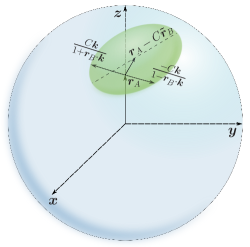
Figure 1: (Color online) Schematic representation of the correlation ellipsoid (20) depicting the possible Bloch vectors $\bm{r}_{A/\bm{k}}$ of the post-measurement state of $A$. It is centered at $\bm{r}_{A}-C\tilde{\bm{r}}_{B}$, with $\tilde{\bm{r}}_{B}=\bm{r}_{B}/(1-r_{B}^{2})$. For a given direction $\bm{k}$ on the unit sphere of $B$, the vectors $\bm{r}_{A/\pm\bm{k}}$ in $A$ are the endpoints of a chord running through $\bm{r}_{A}$. If $\bm{r}_{B}=\bm{0}$, the ellipsoid becomes centered at $\bm{r}_{A}$.

For pure states $\rho_{AB}^{2}=\rho_{AB}$, $\rho_{A/\Pi_{\bm{k}}}$ is pure $\forall$ $\bm{k}$, so that $|\bm{r}_{A/\bm{k}}|^{2}=d_{A}-1$ $\forall$ $\bm{k}$. For instance, in a two-qubit system, by suitable choosing the local $x,y,z$ axes, the Schmidt decomposition allows to write any pure state as $|\Psi_{AB}\rangle=\sqrt{p}|00\rangle+\sqrt{1-p}|11\rangle$. This leads to $C_{\mu\nu}=\delta_{\mu\nu}C_{\mu}$ and $r_{A\mu}=r_{B\mu}=\delta_{\mu z}r_{B}$, with $C_{x}=-C_{y}=2\sqrt{p(1-p)}$, $r_{B}=2p-1$ and $C_{z}=1-r_{B}^{2}=C_{x}^{2}$. It is then verified that for $p\in(0,1)$, the ellipsoid (20) becomes the Bloch sphere of $A$ ($CN_{B}^{-1}C^{T}=(1-r_{B}^{2})I$, $C\tilde{\bm{r}}_{B}=\bm{r}_{A}$).

II.3 The case of the quadratic entropy

II.3.1 Explicit expressions and minimum conditional entropy

The evaluation of $S_{f}(\rho_{A})$ for a general $f$ requires the eigenvalues of $\bm{r}_{A}\cdot\bm{\sigma}_{A}$. However, in the case of the quadratic entropy

$$S_{2}(\rho)=2(1-{\rm Tr}\,\rho^{2})\,,$$ (22)

obtained for $f(p)=p(1-p)$ (also denoted as linear entropy as it follows from the approximation $-\ln p\approx 1-p$ in the von Neumann entropy), a close evaluation in terms of $|\bm{r}_{A}|$ becomes feasible. We obtain, using Eq. (7),

$$S_{2}(\rho_{A})=2\left(1-\frac{1+|\bm{r}_{A}|^{2}}{d_{A}}\right)\,.$$ (23)

Eq. (23) is trivially related to the purity ${\rm Tr}\,\rho_{A}^{2}=(1+|\bm{r}_{A}|^{2})/d_{A}$ and to the standard squared distance to the maximally mixed state, $||\rho_{A}-I_{A}/d_{A}||^{2}=|\bm{r}_{A}|^{2}/d_{A}$, where $||O||^{2}={\rm Tr}\,O^{\dagger}O$. Eq. (23) shows that $|\bm{r}_{A}|^{2}\leq d_{A}-1$, with $|\bm{r}_{A}|^{2}=d_{A}-1$ just for pure states $\rho_{A}^{2}=\rho_{A}$.

Using Eqs. (14), (15) and (23), the conditional entropy (16) in the quadratic case can be expressed as GR.14

$$S_{2}(A|B_{\bm{k}}) = S_{2}(\rho_{A})-\Delta S_{2}(A|B_{\bm{k}})\,,$$ (24)

$$\Delta S_{2}(A|B_{\bm{k}}) = \frac{2}{d_{A}}\frac{|{C}\bm{k}|^{2}}{1-(\bm{r}_{B}\cdot\bm{k})^{2}}=\frac{2}{d_{A}}\frac{\bm{k}^{T}C^{T}C\bm{k}}{\bm{k}^{T}N_{B}\bm{k}}\,,$$ (25)

where $C^{T}C$ and $N_{B}$ (Eq. (19)) are $3\times 3$ positive semi-definite matrices. The entropy decrease (25) is then non-negative and represents the average conditional purity gain due to the measurement on $B$. It is independent of $\bm{r}_{A}$.

Since Eq. (25) is a ratio of quadratic forms, the direction $\bm{k}$ leading to the maximum entropy decrease can be obtained by solving the weighted eigenvalue problem GR.14

$$C^{T}C\bm{k}=\lambda N_{B}\bm{k}\,,$$ (26)

which implies ${\rm Det}[C^{T}C-\lambda N_{B}]=0$, and selecting the eigenvector $\bm{k}$ associated with the largest eigenvalue $\lambda_{\rm max}$. This leads to $\Delta S_{2}(A|B_{\bm{k}})\leq 2\lambda_{\rm max}/d_{A}$ $\forall$ $\bm{k}$, i.e.,

$$\mathop{\rm Min}_{\bm{k}}S_{2}(A|B_{\bm{k}})=S_{2}(\rho_{A})-\frac{2}{d_{A}}\lambda_{\rm max}\,.$$ (27)

We may also express (25) as the quadratic form

$$\Delta S_{2}(A|B_{\bm{k}})=\frac{2}{d_{A}}\bm{k}_{N}^{T}C_{N}^{T}C_{N}\bm{k}_{N}\,,\;\;C_{N}=CN_{B}^{-1/2}\,,$$ (28)

where $\bm{k}_{N}=N_{B}^{1/2}\bm{k}/|N_{B}^{1/2}\bm{k}|$ is a unit vector. Eq. (26) is in fact equivalent to $C_{N}^{T}C_{N}\bm{k}_{N}=\lambda\bm{k}_{N}$, showing that $\sqrt{\lambda_{\rm max}}$ is the maximum singular value of $C_{N}$.

An important final remark is that for this entropy, generalized (POVM) measurements on qubit $B$ cannot decrease the projective minimum (27).

Proof.

For a measurement based on rank one operators $\sqrt{r_{\bm{k}}}\,\Pi_{\bm{k}}^{B}$, $\Pi_{\bm{k}}^{B}=\frac{1}{2}(I_{B}+\bm{k}\cdot\bm{\sigma}_{B})$, with $\sum_{\bm{k}}r_{\bm{k}}\Pi^{B}_{\bm{k}}=I_{B}$, Eq. (17) leads, for $\Delta S_{2}(A|B_{M})\equiv S_{2}(\rho_{A})-S_{2}(A|B_{M})$, to

$$\Delta S_{2}(A|B_{\{r_{\bm{k}}\Pi_{\bm{k}}\}}) = {\frac{1}{d_{A}}}\sum_{\bm{k}}r_{\bm{k}}\frac{|C\bm{k}|^{2}}{1+\bm{r}_{B}\cdot\bm{k}}$$ (29)

$$= \frac{1}{d_{A}}\sum_{\bm{k}}r_{\bm{k}}(1-\bm{r}_{B}\cdot\bm{k})\frac{|C\bm{k}|^{2}}{1-(\bm{r}_{B}\cdot\bm{k})^{2}}$$

$$\leq \frac{\lambda_{\rm max}}{d_{A}}\sum_{\bm{k}}r_{\bm{k}}(1-\bm{r}_{B}\cdot\bm{k})=\frac{2}{d_{A}}\lambda_{\rm max}\,,$$

where we used Eq. (27). This ensures that the lowest conditional entropy (maximum $\Delta S_{2}(A|B_{M})$) is reached for the projective measurement determined by Eq. (26). ∎

II.3.2 Geometrical picture of optimum measurement

Eq. (26) is also the counterpart at $B$ of the eigenvalue Eq. (21) (equivalent to $C_{N}C_{N}^{T}\bm{k}^{A}=\lambda\bm{k}^{A}$), which determined the correlation ellipsoid axes, having both the same non-zero eigenvalues $\lambda_{\mu}$, with related eigenvectors ($C^{T}C\bm{k}=\lambda N_{B}\bm{k}$ $\Rightarrow$ $CN_{B}^{-1}C^{T}\bm{k}^{A}=\lambda\bm{k}^{A}$ for $\bm{k}^{A}\propto C\bm{k}$). Hence, the optimizing measurement of the quadratic entropy is precisely that leading to $\delta\bm{r}_{A}\propto C\bm{k}$ parallel to the major semi-axis of the correlation ellipsoid (Fig. 2).

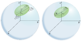
Figure 2: (Color online) Bloch vectors of the post-measurement states of $\bm{A}$ that minimize the quadratic conditional entropy (24). The left panel depicts the general case, whereas the right panel the case $\bm{r}_{B}=\bm{0}$. The increase $\delta{\bm{r}}_{A}=\bm{r}_{A/\bm{k}}-\bm{r}_{A}$ is parallel to the largest semiaxis of the correlation ellipsoid, and coincides with it when $\bm{r}_{B}=\bm{0}$.

If $\bm{r}_{B}=\bm{0}$, the Bloch vector of post-measurement state of $A$ is just $\bm{r}_{A/\pm\bm{k}}=\bm{r}_{A}\pm C\bm{k}$, with equal probabilities for $\bm{k}$ and $-\bm{k}$, and the correlation ellipsoid becomes centered at $\bm{r}_{A}$ (right panel in Fig. 2). Hence, for a given direction $\bm{k}$, the two possible post-measurement Bloch vectors are located diametrically opposite on this ellipsoid. The vector $\bm{k}$ optimizing the quadratic entropy leads then to $\delta\bm{r}_{A}=\pm C\bm{k}$ directly coincident with the major semi-axis, with $\lambda_{\rm max}={\rm max}_{\mu}\{C_{\mu}^{2}\}$, representing its squared length. Note that in this case $N_{B}=I$ and Eq. (26) becomes just $C^{T}C\bm{k}=\lambda\bm{k}$. Hence, the optimizing $\bm{k}$ leads to maximum correlation: $|C\bm{k}|=\sqrt{\bm{k}^{T}C^{T}C\bm{k}}=\sqrt{\lambda_{\rm max}}$, with $|C\bm{k}^{\prime}|\leq|C\bm{k}|$ for any other direction $\bm{k}^{\prime}$.

Since the conditional entropy is a measure of the average uncertainty about $A$ as a result of a measurement on $B$, its minimization implies making use of the maximum amount of correlations available by a measurement on $B$. If the correlation tensor measures the spatial distribution of correlations, the measurement that maximizes correlations access should be in principle that leading to a maximum length of $C\bm{k}$, which is precisely the measurement minimizing the quadratic conditional entropy.

For $\bm{r}_{B}\neq\bm{0}$, the effect of $N_{B}^{-1}$ in Eq. (20) is to deform the $\bm{r}_{B}=\bm{0}$ correlation ellipsoid, expanding it along the direction of $C\bm{r}_{B}$. Accordingly, in Eqs. (25)–(28) $N_{B}$ will favor measurements with $\bm{k}$ along or close to $\bm{r}_{B}$, i.e., in the basis of ${\rho_{B}}$’s eigenstates. In order to understand this result, note that for $\bm{r}_{B}\neq\bm{0}$, $C$ in Eq. (15) acts on vectors $\tilde{\bm{k}}_{\pm}={\pm\bm{k}}/({1\pm\bm{r}_{B}\cdot\bm{k}})$ which have a direction dependent norm and lie on the surface of the shifted ellipsoid (18), making correlation access dependent not only on $C$ but also on $\bm{r}_{B}$. Nonetheless, it is seen from Eq. (18) that vectors $N_{B}^{1/2}\tilde{\bm{k}}_{\pm}$ lie on a shifted sphere, forming a chord that passes through the origin. The origin will divide this chord in two segments whose length’s product is $|N_{B}^{1/2}\tilde{\bm{k}}_{+}||N_{B}^{1/2}\tilde{\bm{k}}_{-}|=\frac{\bm{k}^{T}N_{B}\bm{k}}{1-(r_{B}\cdot\bm{k})^{2}}=1$.

Since $C\tilde{\bm{k}}_{\pm}=C_{N}N_{B}^{1/2}\tilde{\bm{k}}_{\pm}$ (Eq. (28)), the ellipsoid (20) may be seen as the image of the previous sphere under the linear transformation $C_{N}$. As before, if $C_{N}$ measures the effective spatial distribution of correlations, the product

$$|C_{N}(N_{B}^{1/2}\tilde{\bm{k}}_{+})||C_{N}(N_{B}^{1/2}\tilde{\bm{k}}_{-})|=\frac{|C\bm{k}|^{2}}{1-(\bm{r}_{B}\cdot\bm{k})^{2}}\,,$$

which is just proportional to $\Delta S_{2}(A|B_{\bm{k}})$ (Eq. (25)), is a measure of correlations along direction $\bm{k}$ at $B$. The direction $\bm{k}$ that minimizes $S_{2}(A|B_{\bm{k}})$ is then precisely that which maximizes this product.

II.4 Conditional entropy and optimal measurement in the weakly correlated limit

We now discuss the main general result of this manuscript. We will extend the previous results to a general entropy $S_{f}$, within the weakly correlated regime. This regime refers to the case where the correlation ellipsoid (Fig. 1) is sufficiently small: $|\delta\bm{r}_{A}|=|\frac{C\bm{k}}{1\pm\bm{r}_{B}\cdot\bm{k}}|\ll 1$ $\forall$ $\bm{k}$ in (15). In this situation, we may consider an expansion of the conditional entropy (16) around $\rho_{A}$, up to second order in $\delta\rho_{A}=\delta\bm{r}_{A}\cdot\bm{\sigma}_{A}/d_{A}$. The result is

$$S_{f}(A|B_{\bm{k}})\approx S_{f}(\rho_{A})-\frac{2}{d_{A}}\frac{\bm{k}^{T}C^{T}\Lambda_{f}(\rho_{A})C\bm{k}}{\bm{k}^{T}N_{B}\bm{k}}\,,$$ (30)

where $N_{B}$ is the $3\times 3$ matrix (19) and $\Lambda_{f}(\rho_{A})$ denotes a scaled $D_{A}\times D_{A}$ Hessian matrix, of elements

$$[\Lambda_{f}(\rho_{A})]_{\mu\mu^{\prime}} = \frac{1}{4d_{A}}\sum_{i,j}R_{ij}\langle i|\sigma_{A\mu}|j\rangle\langle j|\sigma_{A\mu^{\prime}}|i\rangle\,,$$ (31)

$$R_{ij} = {(1-\delta_{ij})\frac{f^{\prime}(p^{A}_{i})-f^{\prime}(p^{A}_{j})}{p^{A}_{j}-p^{A}_{i}}-\delta_{ij}f^{\prime\prime}(p_{i}^{A})}\,,$$ (32)

where $\rho_{A}|i\rangle=p_{i}^{A}|i\rangle$. Actually, just the $3\times 3$ submatrix of $\Lambda_{f}(\rho_{A})$ corresponding to the three principal directions selected by $C$ in Eq. (12), is actually required in (30).

Proof.

We start from the second order expansion of the eigenvalues $p_{i/\bm{k}}^{A}$ of the post-measurement state (13),

$$p^{A}_{i/\bm{k}}\approx p_{i}^{A}+\langle i|\delta\rho_{A}|i\rangle+\sum_{j\neq i}\frac{|\langle j|\delta\rho_{A}|i\rangle|^{2}}{p^{A}_{i}-p^{A}_{j}}\,,$$ (33)

where $p_{i}^{A}$ are those of $\rho_{A}$ and $\delta\rho_{A}=\frac{1}{d_{A}}\frac{\pm C\bm{k}}{1\pm\bm{r}_{B}\cdot\bm{k}}\cdot\bm{\sigma}_{A}$. The ensuing second order expansion of the entropy in (16),

$$S_{f}(\rho_{A/\Pi_{\bm{k}}})\approx S_{f}(\rho_{A})+\sum_{i}[f^{\prime}(p^{A}_{i})\delta p^{A}_{i}+\frac{1}{2}f^{\prime\prime}(p^{A}_{i})\delta p^{A\;2}_{i}]\,,$$ (34)

where $\delta p^{A}_{i}=p^{A}_{i/\bm{k}}-p_{i}^{A}$, leads then to Eqs. (30)–(32), after using (33) and neglecting higher order terms. Note that $R_{ij}=-f^{\prime\prime}(p_{ij}^{*})$, with $p_{ij}^{*}$ between $p_{i}^{A}$ and $p_{j}^{A}$, entailing $R_{ij}>0$ $\forall$ $i,j$, with $R_{ij}\rightarrow-f^{\prime\prime}(p_{i})$ if $p_{j}\rightarrow p_{i}$. If $p_{i}^{A}>0$ $\forall$ $i$, $R_{ij}$ is finite $\forall$ $i,j$ for any $f$ of the form considered. ∎

The positivity of $R_{ij}$ $\forall$ $i,j$ implies that $\Lambda_{f}(\rho_{A})$ is positive definite, and hence that $C^{T}\Delta_{f}(\rho_{A})C$ is positive semidefinite. The entropy decrease

$$\Delta S_{f}(A|B_{\bm{k}})=S_{f}(A)-S_{f}(A|B_{\bm{k}})\approx\frac{2}{d_{A}}\frac{\bm{k}^{T}C^{T}\Lambda_{f}(\rho_{A})C\bm{k}}{\bm{k}^{T}N_{B}\bm{k}}$$ (35)

then remains non-negative in the present approximation.

In the case of the quadratic entropy, $R_{ij}=4$ $\forall$ $i,j$, and Eqs. (7) and (31) lead to $\Lambda_{2}(\rho_{A})=I$, reducing Eq. (30) to Eqs. (24)-(25). On the other hand, for $\bm{r}_{A}\rightarrow\bm{0}$ (maximally mixed $\rho_{A}$), $p_{i}^{A}=1/d_{A}$ $\forall$ $i$ and $R_{ij}\rightarrow-f^{\prime\prime}(1/d_{A})$ $\forall$ $i,j$, implying that Eq. (31) becomes again proportional to the identity matrix $\forall$ $S_{f}$:

$$\Lambda_{f}(I_{A}/d_{A})={\textstyle\frac{1}{4}}|f^{\prime\prime}(1/d_{A})|\,I\,.$$ (36)

Hence, Eqs. (35)–(36) lead to $\Delta S_{f}(A|B_{\bm{k}})\propto\Delta_{2}(A|B_{\bm{k}})$ $\forall$ $S_{f}$. In this limit the measurement minimizing $S_{f}(A|B_{\bm{k}})$ is then universal, i.e., the same as that optimizing the quadratic entropy $\forall$ $S_{f}$.

In the general case, the matrix (31) will introduce an additional “anisotropy”, which will depend on $\rho_{A}$ and the choice of $f$, and which represents the effect of the “concavity excess” of $S_{f}$ at $\rho_{A}$ in comparison with that of the quadratic entropy. Nonetheless, Eq. (30) shows that in the weakly correlated regime, $S_{f}(A|B_{\bm{k}})$ becomes equivalent to the quadratic conditional entropy (24) for an effective “deformed” correlation tensor

$$C_{f}=\sqrt{\Lambda_{f}(\rho_{A})}\,C\,.$$ (37)

Minimization of Eq. (30) over $\bm{k}$ then leads again to a $3\times 3$ weighted eigenvalue problem,

$$C^{T}\Lambda_{f}(\rho_{A})C\bm{k}=\lambda_{f}N_{B}\bm{k}\,,$$ (38)

implying ${\rm Det}[C^{T}\Lambda_{f}(\rho_{A})C-\lambda N_{B}]=0$. The minimum is obtained for $\bm{k}$ along the direction of the eigenvector associated with the largest eigenvalue $\lambda_{f{\rm max}}$ of (38):

$$\mathop{\rm Min}_{\bm{k}}S_{f}(A|B_{\bm{k}})\approx S_{f}(\rho_{A})-\frac{2}{d_{A}}\lambda_{f{\rm max}}\,.$$ (39)

Moreover, Eq. (35) can be rewritten as

$$\Delta S_{f}(A|B_{\bm{k}})\approx\frac{2}{d_{A}}\bm{k}_{N}^{T}C_{N}^{T}\Lambda_{f}(\rho_{A})C_{N}\bm{k}_{N}\,,$$ (40)

with $C_{N}$ and $\bm{k}_{N}$ defined as in (28).

The geometric picture of these results is, therefore, similar to that for the quadratic entropy, after replacing $C$ with the deformed correlation tensor (37). As in the quadratic case, in the approximation (34) POVM measurements will not decrease the projective minimum (LABEL:Sfgmin). The argument is the same as that of Eq. (29), after replacing $C$ with $C_{f}$.

II.5 The two-qubit case

Let us now examine the case $d_{A}=2$. The entropy $S_{f}(\rho_{A})$ of a general single qubit state $\rho_{A}=\frac{1}{2}(I_{A}+\bm{r}_{A}\cdot\bm{\sigma})$ will depend just on the length of the Bloch vector $\bm{r}_{A}$:

$$S_{f}(\rho_{A})=\sum_{\nu=\pm 1}f({\textstyle\frac{1+\nu|\bm{r}_{A}|}{2}})=h_{f}(|\bm{r}_{A}|),$$ (41)

where $h_{f}(r)$ is a concave strictly decreasing function of $r$ for any strictly concave $f$. The conditional entropy (16) can then be written as

$$S_{f}(A|B_{\bm{k}})=\sum_{\nu=\pm 1}p_{\nu\bm{k}}\,h_{f}\left(\left|\bm{r}_{A}+\nu\frac{C\bm{k}}{1+\nu\bm{r}_{B}\cdot\bm{k}}\right|\right)\,,$$ (42)

where $C$ is now a $3\times 3$ matrix.

If $\bm{r}_{A}=\bm{r}_{B}=\bm{0}$ (maximally mixed marginals), Eq. (42) reduces to

$$S_{f}(A|B_{\bm{k}})=h_{f}(|C\bm{k}|)\;\;\;\;(\bm{r}_{A}=\bm{r}_{B}=\bm{0})\,.$$ (43)

Hence, in this case its minimum is reached, for any $S_{f}$, for that $\bm{k}$ which maximizes $|C\bm{k}|$, i.e.,

$$\mathop{\rm Min}_{\bm{k}}S_{f}(A|B_{\bm{k}})=h_{f}(\sqrt{\lambda_{\rm max}})\;\;\;\;(\bm{r}_{A}=\bm{r}_{B}=\bm{0})\,,$$ (44)

where $\lambda_{\rm max}$ is the largest eigenvalue of $C^{T}C$ and $\bm{k}$ the associated eigenvector ($\sqrt{\lambda_{\rm max}}=C_{\rm max}$ is the largest singular value of $C$). Non-projective measurements will not decrease this value, since $h_{f}(|C\bm{k}|)\geq h_{f}(\sqrt{\lambda_{\rm max}})$ $\forall$ $\bm{k}$. Hence, there is in this case an exact universal optimizing measurement, determined by the largest semi-axis of the correlation ellipsoid.

Let us now consider the weakly correlated regime. In the two-qubit case, Eqs. (30) and (41) lead to

$$S_{f}(A|B_{\bm{k}})\approx h_{f}(|\bm{r}_{A}|)-\frac{\bm{k}^{T}C^{T}\Lambda_{f}(\bm{r}_{A})C\bm{k}}{\bm{k}^{T}N_{B}\bm{k}}\,,$$ (45)

where the Hessian matrix (31) becomes now a $3\times 3$ matrix that depends just on $\bm{r}_{A}$ and can be expressed as

$$\Lambda_{f}(\bm{r}_{A}) = -\frac{h^{\prime}_{f}(r_{A})}{2r_{A}}\left[I+[\eta_{f}(r_{A})-1]\frac{\bm{r}_{A}\bm{r}_{A}^{T}}{r_{A}^{2}}\right]\,,$$ (46)

$$\eta_{f}(r) = rh_{f}^{\prime\prime}(r)/h_{f}^{\prime}(r)\,,$$ (47)

where $r_{A}=|\bm{r}_{A}|$. It is then verified that for $f$ concave, $\Lambda_{f}(\bm{r}_{A})$ is a positive definite $3\times 3$ matrix, since $\eta_{f}(r)>0$.

For the quadratic entropy, $h_{f}(r)=\frac{1-r^{2}}{2}$ and $\eta_{f}(r)=1$, implying $\Lambda_{f}(\bm{r}_{A})=I$. It is also verified that for $\bm{r}_{A}\rightarrow\bm{0}$ and arbitrary $S_{f}$, $h_{f}^{\prime}(r_{A})\rightarrow 0$, with $h_{f}^{\prime}(r_{A})/r_{A}\rightarrow h_{f}^{\prime\prime}(0)$ and $\eta_{f}(r_{A})\rightarrow 1$, implying $\Lambda_{f}(\bm{0})=\frac{1}{2}|h^{\prime\prime}_{f}(0)|I$, in agreement with (36). In this limit $\Delta S_{f}(A|B_{\bm{k}})\approx\frac{1}{2}|h_{f}^{\prime\prime}(0)|\Delta S_{2}(A|B_{\bm{k}})$ $\forall$ $S_{f}$ in the approximation (45).

However, for a general $\bm{r}_{A}$, $\Lambda_{f}(\bm{r}_{A})$ will introduce an anisotropy in the direction of $\bm{r}_{A}$ whenever $\eta_{f}(r_{A})\neq 1$. This factor is a local measure of the concavity of $h_{f}$ in the direction of $\bm{r}_{A}$, taking as reference the quadratic entropy, and will favor the $\bm{r}_{A}$ direction if $\eta_{f}(r_{A})>1$. This occurs in the Von Neumann case (Fig. 3), where $h_{f}(r)=h(r)=-\sum_{\nu=\pm 1}\frac{1+\nu r}{2}\log_{2}\frac{1+\nu r}{2}$ and $\eta_{f}(r)=\eta(r)$, with

$$\eta(r)=\frac{2r}{(1-r^{2})\ln\frac{1+r}{1-r}}>1\,,$$ (48)

for $r>0$ ($\eta(r)\approx 1+2r^{2}/3$ for $r\rightarrow 0$). However, $\eta_{f}(r)<1$ is also possible for a general concave $f$. For instance, for the Tsallis entropies TS.09 $S_{q}(\rho)=(1-{\rm Tr}\,\rho^{q})/c_{q}$, obtained for $f(p)=(p-p^{q})/c_{q}$, with $c_{q}=1-2^{1-q}$ and $q>0$,

$$\eta_{q}(r)=\frac{(q-1)r}{1+r}\frac{1+\gamma^{q-2}}{1-\gamma^{q-1}}\,,$$

where $\gamma=\frac{1-r}{1+r}$. This leads to $\eta_{q}(r)>1$ for $q\in(0,2)$ or $q>3$ but $\eta_{q}(r)<1$ for $q\in(2,3)$, with $\eta_{q}(r)=1$ for $q=2$ or $q=3$ ($\eta_{q}(r)\approx 1+\frac{(q-2)(q-3)}{3}r^{2}$ for $r\rightarrow 0$). Note that $S_{q}(\rho)$ becomes the von Neumann entropy for $q\rightarrow 1$ and the quadratic entropy (22) for $q=2$, coinciding again with $S_{2}(\rho)$ for $q=3$ in the single qubit case RCC.10 .

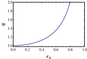
Figure 3: (Color online) Plot of the factor $\eta(r_{A})=\frac{r_{A}h^{\prime\prime}(r_{A})}{h^{\prime}(r_{A})}$ in Eq. (46) for the von Neumann entropy. Since it is an increasing function, differences with the quadratic entropy results (for which $\eta(r_{A})=1$ $\forall$ $r_{A}$) will increase as $r_{A}=|\langle\bm{\sigma}_{A}\rangle|$ increases. Quantities plotted are dimensionless.

We can now easily understand the main features of the projective measurement minimizing $S_{f}(A|B_{\bm{k}})$ for a general $S_{f}$. For maximally mixed marginal states, correlation access depends solely on the correlation tensor, and the maximum correlation direction, i.e., the major axis of the correlation ellipsoid, is preferred $\forall$ $S_{f}$. This preference is affected by a non zero value of $\bm{r}_{B}$, which introduces an anisotropic normalization on the measurement vectors and entails the replacement of $C$ by $C_{N}=CN_{B}^{-1/2}$, which will favor the direction of $\bm{r}_{B}$. Finally, for $\bm{r}_{A}\neq\bm{0}$ the local concavity induces an additional $f$-dependent anisotropy around the direction of $\bm{r}_{A}$, which in the weakly correlated regime amounts to replace $C_{N}$ by $\sqrt{\Lambda_{f}(\bm{r}_{A})}C_{N}$. For $r_{B}\rightarrow 1$ or in the pure state limit, the approximation (45) will normally break down, since the correlation ellipsoid will typically become large.

Measurement equivalent. In a two-qubit system, the conditional entropy decrease at $A$ due to a measurement on $B$ can be characterized by an effective Bloch vector length increase $\Delta_{f}$ at $A$, which we will denote as measurement equivalent. For a projective measurement, it is defined by (Fig. 4)

$$h_{f}(|\bm{r}_{A}|+\Delta_{f})=S_{f}(A|B_{\bm{k}})\,.$$ (49)

Since $S_{f}(A|B_{\bm{k}})\leq S_{f}(A)$, $\Delta_{f}\geq 0$ for $f$ concave, increasing as $\bm{k}$ approaches the optimal direction.

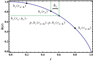
Figure 4: (Color online) A measurement is performed in the direction of vector $\bm{k}$ on qubit $B$ and the entropy of the post-measurement state of $A$ as measured by $S_{f}$ is $h_{f}(|\bm{r}_{A/\pm\bm{k}}|)$. The measurement equivalent $\Delta_{f}$ is defined as the increase in the norm of vector $\bm{r}_{A}$ that satisfies $h_{f}(\bm{r}_{A}+\Delta_{f})=p_{\bm{k}}h_{f}(|\bm{r}_{A/\bm{k}}|)+p_{-\bm{k}}h_{f}(|\bm{r}_{A/-\bm{k}}|)$ ($h$ and $r$ dimensionless).

In the weakly correlated regime, $\Delta_{f}$ will be small. If $\bm{r}_{A}\neq\bm{0}$, we then have $h_{f}(r_{A}+\Delta_{f})\approx h_{f}(r_{A})+h^{\prime}_{f}(r_{A})\Delta_{f}$, and Eq. (45) leads to $\Delta_{f}$ of order $||C_{N}||^{2}$:

$$\Delta_{f} \approx \frac{1}{|h^{\prime}_{f}(r_{A})|}\frac{\bm{k}^{T}C^{T}\Lambda_{f}(\bm{r}_{A})C\bm{k}}{\bm{k}^{T}N_{B}\bm{k}}\,\;\;(r_{A}>0).$$ (50)

On the other hand, if $\bm{r}_{A}\rightarrow\bm{0}$, $h^{\prime}_{f}(0)=0$ and we have instead $h_{f}(\Delta_{f})\approx h_{f}(0)+\frac{1}{2}h^{\prime\prime}_{f}(0)\Delta^{2}_{f}$. Since $\Lambda_{f}(\bm{0})=\frac{1}{2}|h^{\prime\prime}_{f}(0)|I$, Eq. (45) leads in this case to

$$\Delta_{f} \approx \sqrt{\frac{\bm{k}^{T}C^{T}C\bm{k}}{\bm{k}^{T}N_{B}\bm{k}}}=\frac{|C\bm{k}|}{\sqrt{1-(\bm{r}_{B}\cdot\bm{k})^{2}}}\,\;\;(\bm{r}_{A}=0).$$ (51)

Thus, for $\bm{r}_{A}\rightarrow\bm{0}$, $\Delta_{f}$ becomes independent of $f$ (universal limit) and of order $||C_{N}||$.

III Application

III.1 Quantum discord estimation

Given a bipartite quantum state $\rho_{AB}$ with marginal states $\rho_{A(B)}$, the quantum discord for a local measurement on $B$ can be written as OZ.01

$$D(A|B) = \mathop{\rm Min}_{\{\Pi_{j}\}}D(A|B_{\{\Pi_{j}\}}),$$ (52)

$$D(A|B_{\{\Pi_{j}\}}) = S(A|B_{\{\Pi_{j}\}})-[S(\rho_{AB})-S(\rho_{B})]$$ (53)

where $S(A|B_{\{\Pi_{j}\}})$ is the conditional entropy (1) in the von Neumann case, with the minimum in (52) taken over all possible measurements on $B$, while the bracket in (53) is the measurement independent quantum conditional entropy. We may also rewrite (53) as

$$D(A|B_{\{\Pi_{j}\}})=I(A,B)-\Delta S(A|B_{\{\Pi_{j}\}})\,,$$ (54)

where $\Delta S(A|B_{\{\Pi_{j}\}})=S(A)-S(A|B_{\{\Pi_{j}\}})$ and

$$I(A,B)=S(\rho_{A})+S(\rho_{B})-S(\rho_{AB})\,,$$ (55)

is the quantum mutual information.

For qudit-qubit systems, the results of previous section can be applied to estimate Eqs. (52)-(54) in the weakly correlated regime. For a projective measurement along direction $\bm{k}$ at $B$, Eq. (35) leads to

$$D(A|B_{\bm{k}})\approx I(A,B)-\frac{2}{d_{A}}\frac{\bm{k}^{T}C^{T}\Lambda(\rho_{A})C\bm{k}}{\bm{k}^{T}N_{B}\bm{k}},$$ (56)

where $\Lambda(\rho_{A})$ is the Hessian matrix (31) in the von Neumann case. The minimization in (52) leads then to the eigenvalue problem (38), and the minimum reads

$$D(A|B)\approx I(A,B)-\frac{2}{d_{A}}\lambda_{\rm max},$$ (57)

with $\lambda_{\rm max}$ the largest root of ${\rm Det}[C^{T}\Lambda(\rho_{A})C-\lambda N_{B}]=0$. While $I(A,B)$ is a measure of the total correlation between $A$ and $B$, the second term in (57) represents the maximum classical-like mutual information obtained after a local measurement on $B$, in the present regime.

In this regime we may also apply a quadratic approximation to (55) using the representation (8) of $\rho_{AB}$. An expansion of $S(\rho_{AB})$ up to second order in the correlation tensor $C$, extending Eqs. (33)–(34) to this case ($|i\rangle\rightarrow|i_{A}j_{B}\rangle$, $p_{i}^{A}\rightarrow p_{i}^{A}p_{j}^{B}$, $\delta\rho_{A}\rightarrow\delta\rho_{AB}=\rho_{AB}-\rho_{A}\otimes\rho_{B}$, with $\rho_{A(B)}|i_{A(B)}\rangle=p_{i}^{A(B)}|i_{A(B)}\rangle$), leads to

$$I(A,B) \approx \frac{1}{2}\bm{C}^{T}\Lambda(\rho_{A},\rho_{B})\bm{C}\,,$$ (58)

where $\bm{C}$ denotes a vector of elements $C_{\mu\nu}$ and $\Lambda$ is here the $3D_{A}\times 3D_{A}$ matrix

$$\Lambda_{\mu\nu}^{\mu^{\prime}\nu^{\prime}}(\rho_{A},\rho_{B}) = {\textstyle\frac{1}{4d_{A}^{2}}\sum\limits_{i,j,k,l}R_{ik}^{jl}\langle i_{A}|\sigma_{A\mu^{\prime}}|j_{A}\rangle\langle j_{A}|\sigma_{A\mu}|i_{A}\rangle}$$ (59)

$${\times\langle k_{B}|\sigma_{B\nu^{\prime}}|l_{B}\rangle\langle l_{B}|\sigma_{B\nu}|k_{B}\rangle}\,,$$

$$R_{ik}^{jl} = {\textstyle\frac{1}{\ln 2}[(1-\delta_{i}^{j}\delta_{k}^{l})\frac{\ln[p_{i}^{A}p_{k}^{B}/(p_{j}^{A}p_{l}^{B})]}{p_{i}^{A}p_{k}^{B}-p_{j}^{A}p_{l}^{B}}+\delta_{i}^{j}\delta_{k}^{l}\frac{1}{p_{i}^{A}p_{k}^{B}}}]\,.$$

The terms linear in $C$ vanish for the von Neumann entropy. Eq. (56) becomes then a quadratic form in the elements of the correlation tensor, which is positive semidefinite since $D(A|B)\geq 0$ and the quadratic approximation becomes exact for sufficiently small $C$.

The decomposition (12) allows to reduce Eq. (58) to a quadratic form in the three singular values $C_{\mu}$. For instance, for maximally mixed marginals, $R^{jl}_{ik}=2d_{A}/\ln 2$ $\forall$ $i,j,k,l$, implying $\Lambda^{\mu\nu}_{\mu^{\prime}\nu^{\prime}}(\frac{I_{A}}{d_{A}},\frac{I_{B}}{2})=\frac{1}{\ln 2}\delta^{\mu}_{\mu^{\prime}}\delta^{\nu}_{\nu^{\prime}}$. Eq. (58) then reduces to $I(A,B)\approx\frac{1}{2\ln 2}{\rm Tr}\,C^{T}C=\frac{1}{2\ln 2}\sum_{\mu=1}^{3}C_{\mu}^{2}$.

III.2 Two-qubit states with $\bm{r}_{A}$ and $\bm{r}_{B}$ parallel to a principal axis of $C$

In the special two-qubit case where $\bm{r}_{A}$ and $\bm{r}_{B}$ are parallel to one of the principal directions selected by $C$ in the diagonal representation (12) (implying that they should be eigenvectors of $CC^{T}$ and $C^{T}C$ respectively), tensors $\Lambda_{f}(\bm{r}_{A})$, $C$ and $N_{B}=I-\bm{r}_{B}\bm{r}_{B}^{T}$ can be made simultaneously diagonal: We may choose the local orthogonal $x,y,z$ axes at $A$ and $B$ such that for $\mu,\nu=x,y,z$,

$$C_{\mu\nu}=\delta_{\mu\nu}C_{\mu}\,,$$ (60)

with $C_{\mu}$ the singular values of $C$ and $\bm{r}_{A}$ and $\bm{r}_{B}$ parallel to one of these axes. Eqs. (26) and (38) then imply that the optimal measurement minimizing the conditional entropy in the weakly correlated regime (and in all cases for the quadratic entropy) is to be found among these principal axes.

If $\bm{r}_{A}$ and $\bm{r}_{B}$ are both directed along $\bm{z}$ (i.e., $\bm{r}_{A}\propto C\bm{r}_{B}$), Eqs.  (35), (46) and (60) lead to

$$\Delta S_{f}(A|B_{\bm{k}})\approx{\textstyle\frac{|h^{\prime}_{f}(r_{A})|}{2r_{A}}\,\frac{C_{x}^{2}{k}_{x}^{2}+C_{y}^{2}{k}_{y}^{2}+\eta_{f}(r_{A})C_{z}^{2}k_{z}^{2}}{1-r_{B}^{2}k_{z}^{2}}}\,,$$ (61)

with its maximum then given by

$$\mathop{\rm Max}_{\bm{k}}\Delta S_{f}(A|B_{\bm{k}})\approx{\textstyle\frac{|h^{\prime}_{f}(r_{A})|}{2r_{A}}{\rm Max}[C_{x}^{2},C_{y}^{2},\frac{\eta_{f}(r_{A})}{1-r_{B}^{2}}C_{z}^{2}]}\,.$$ (62)

On the other hand, if $\bm{r}_{A}$ and $\bm{r}_{B}$ are along orthogonal principal axes ($\bm{r}_{A}\perp C\bm{r}_{B}$), for instance $\bm{r}_{B}$ along $\bm{z}$ and $\bm{r}_{A}$ along $\bm{x}$, we obtain instead

$$\Delta S_{f}(A|B_{\bm{k}})\approx{\textstyle\frac{|h^{\prime}_{f}(r_{A})|}{2r_{A}}\,\frac{\eta_{f}(r_{A})C_{x}^{2}{k}_{x}^{2}+C_{y}^{2}{k}_{y}^{2}+C_{z}^{2}k_{z}^{2}}{1-r_{B}^{2}k_{z}^{2}}}\,,$$ (63)

with its maximum given by

$$\mathop{\rm Max}_{\bm{k}}\Delta S_{f}(A|B_{\bm{k}})\approx{\textstyle\frac{|h^{\prime}_{f}(r_{A})|}{2r_{A}}{\rm Max}[\eta_{f}(r_{A})C_{x}^{2},C_{y}^{2},\frac{C_{z}^{2}}{1-r_{B}^{2}}]}\,.$$ (64)

For use in the next subsection, we quote here the explicit expressions for the case of the von Neumann entropy when $\bm{r}_{A}$ and $\bm{r}_{B}$ are both parallel to $\bm{z}$. We obtain

$$\Delta S(A|B_{\bm{k}})\approx{\textstyle\frac{\frac{1}{2r_{A}}\ln\frac{1+r_{A}}{1-r_{A}}(C_{x}^{2}{k}_{x}^{2}+C_{y}^{2}{k}_{y}^{2})+\frac{1}{1-r_{A}^{2}}C_{z}^{2}k_{z}^{2}}{2\ln 2\,(1-r_{B}^{2}k_{z}^{2})}}\,,$$ (65)

whereas the quadratic approximation (58) becomes

$$I(A,B) \approx {\textstyle\frac{1}{2\ln 2}}[\!{\textstyle\sum\limits_{\nu=\pm 1}\!\frac{(C_{x}-\nu C_{y})^{2}\ln(\frac{1+r_{A}}{1-r_{A}}\,\frac{1+\nu r_{B}}{1-\nu r_{B}})}{4(r_{A}+\nu r_{B})}}+{\textstyle\frac{C_{z}^{2}}{(1-r_{A})^{2}(1-r_{B})^{2}}]}\,.$$

It is verified that within the approximations (65)–(LABEL:Ia), $D(A|B_{\bm{k}})=I(A,B)-\Delta S(A|B_{\bm{k}})$ becomes a non-negative quadratic form in the $C_{\mu}$’s.

III.3 Optimum measurement for $X$ states

We now apply previous approximations to the set of two-qubit $X$ states, which arise naturally in many physical situations BL.08 ; RD.08 ; CRC.10 . Through the singular value decomposition of the tensor $J_{\mu\nu}=\langle\sigma_{\mu}\otimes\sigma_{\nu}\rangle$, and by suitably choosing the local bases, these states can be written as

$$\rho_{AB} = \frac{1}{4}(I\otimes I+r_{A}\sigma_{z}\otimes I+r_{B}I\otimes\sigma_{z}+\sum_{\mu}J_{\mu}\sigma_{\mu}\otimes\sigma_{\mu})$$ (67)

$$= \left(\begin{array}[]{cccc}p_{+}&0&0&\alpha_{-}\\ 0&q_{+}&\alpha_{+}&0\\ 0&\alpha_{+}&q_{-}&0\\ \alpha_{-}&0&0&p_{-}\end{array}\right);\begin{array}[]{c}p_{\pm}=\frac{1\pm(r_{A}+r_{B})+J_{z}}{4}\\ q_{\pm}=\frac{1\pm(r_{A}-r_{B})-J_{z}}{4}\\ \alpha_{\pm}=\frac{J_{x}\pm J_{y}}{4}\end{array}$$ (75)

with (75) the state representation in the standard basis. The parameters should fulfill the positivity conditions $p_{\pm}\geq 0$, $q_{\pm}\geq 0$, $|\alpha_{-}|\leq\sqrt{p_{+}p_{-}}$, $|\alpha_{+}|\leq\sqrt{q_{+}q_{-}}$, with $p_{+}+p_{-}+q_{+}+q_{-}=1$. Since the correlation tensor $C=J-\bm{r}_{A}\bm{r}_{B}^{T}$ will satisfy Eq. (60), with

$$C_{x}=J_{x}\,,\;\;\;C_{y}=J_{y}\,,\;\;\;C_{z}=J_{z}-r_{A}r_{B}\,,$$

it is clear that in these states the marginal Bloch vectors $\bm{r}_{A}$ and $\bm{r}_{B}$ lie on the same principal axis ($z$) of $C$, implying that these states correspond to the case of Eq. (61). In the weakly correlated limit $S_{f}(A|B_{\bm{k}})$ will then reach its minimum for a measurement along the direction of one of these principal axes (Eq. (62)).

In this regime the minimizing measurement depends not only on $C$ and $r_{B}$, but also on the local concavity of the function $h_{f}(r)$ at $r=|\bm{r}_{A}|$. This implies, in general, that different entropies may reach their minimum value for measurements on different axes. We will now compare the minimizing measurements of the von Neumann and quadratic conditional entropies for states with $J_{x}=J_{y}$, for which the minimizing measurement is either along the $z$ axis or along any vector in the $x,y$ plane, which we will take as $x$. A transition zone between these two directions arises, that will depend on the concavity of the entropy. From Eq. (62) it follows that the transition zone is

$$C_{x}^{2}=\eta_{f}(r_{A})C_{z}^{2}/(1-r_{B}^{2}),$$ (76)

with $\eta_{f}(r_{A})=1$ for the quadratic entropy and $\eta_{f}(r)=\eta(r)$, Eq. (48), for the von Neumann entropy. Since $\eta(r_{A})>1$ for $r_{A}\neq 0$, it is seen that in the von Neumann case, the transition zone is shifted from that of the quadratic entropy whenever $r_{A}\neq 0$, and this discrepancy will increase as $r_{A}$ increases, favoring the $z$ direction.

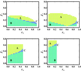
Figure 5: (Color online) Comparison between the projective minimizing measurements for the von Neumann and quadratic conditional entropies, for $X$ states (Eq. (67)) with $r_{B}=0.25$ and $J_{z}=0.3$ (top left), 0.15 (top right), -0.25 (bottom left), -0.5 (bottom right). Yellow (sector A) and green (sector B) disks show the set of states where the minimizing measurement is the same for both entropies (along $\bm{x}$ in A and along $\bm{z}$ in B), while blue disks (C) show those states where the minimizing measurements differ ($J_{x}$ and $r_{A}$ dimensionless).

Typical results for the projective minimizing measurement for these entropies are shown in Fig. 5 as a function of $r_{A}$ and $J_{x}=C_{x}$, for fixed $r_{B}$ and different values of $J_{z}$. It is seen that they are coincident for most states, differing only in the transition region C (blue disks), where the measurement minimizing the quadratic entropy has already changed from $\bm{z}$ to the $\bm{x}$ direction, but the von Neumann entropy still reaches its minimum value for a measurement along $\bm{z}$. As expected, the region of discrepancy becomes greater as $r_{A}$ increases. We should mention that while the $\bm{z}\rightarrow\bm{x}$ transition as $J_{x}$ increases is always sharp for the quadratic conditional entropy, as follows from Eq. (25), in the von Neumann case it may be softened through intermediate measurement directions in a tiny interval of $J_{x}$ values, an effect not seen in the approximation (61)–(65). Actually, in these tiny crossover intervals non-projective measurements can be preferred CZ.11 ; KS.13 (if a projective measurement optimizes the von Neumann conditional entropy for an $X$ state, it should be along a principal axes of $C$ KS.13 ), although differences with the projective minimum are small.

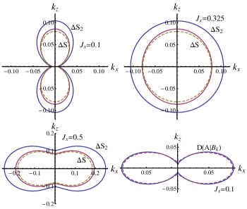
Figure 6: (Color online) The entropy decrease $\Delta S_{f}=S(A)-S(A|B_{\bm{k}})$ after a local measurement on $B$ along direction $\bm{k}=(k_{x},0,k_{z})$ for the quadratic ($\Delta S_{2}$) and von Neumann ($\Delta S$) entropies, together with the quadratic approximation (61)–(65) for the latter (dashed lines). We have considered an $X$ state with $r_{A}=r_{B}=0.25$, $J_{z}=-0.25$ and $J_{x}=0.1,0.325,0.5$, corresponding to states in sectors B, C, and A, respectively, of the lower left panel of Fig. 5. The bottom right panel depicts the quantum discord (54) and its quadratic approximation (65)–(LABEL:Ia) (dashed line) for $J_{x}=0.1$ (quantities plotted dimensionless).

Fig. 6 shows the entropy decrease (“information gain”) $\Delta S_{f}=S_{f}(A)-S_{f}(A|B_{\bm{k}})$ as a function of the direction $\bm{k}=(k_{x},0,k_{z})$ of the measurement on $B$, for $X$ states located below, at and above the transition zone in the bottom left panel of Fig. 5. Both the quadratic and von Neumann conditional entropies are depicted, which are seen to exhibit typically the same profile, together with the second order approximation (65) to the latter, which is seen to provide a good estimation. While there is a clear preference for the $\bm{z}$ ($\bm{x}$) direction for low (high) $J_{x}$, the anisotropy of $\Delta S_{f}$ in the transition region ($J_{x}=0.325$), where the minimizing measurement directions of the von Neumann and quadratic entropies differ, is very small, entailing that this difference is not too relevant. We also depict illustrative results for the discord (54) and its quadratic estimation obtained with Eqs. (65)–(LABEL:Ia), which is quite accurate in the case considered.

IV Conclusions

We have shown that the problem of conditional entropy optimization in a qudit-qubit system, for a general entropic form and a measurement on the qubit, can be solved analytically in the limit of weak correlations. It just requires the solution of a $3\times 3$ eigenvalue problem determined by the correlation tensor of the system, the Bloch vector of the qubit and a local concavity term depending on the choice of entropy (Eqs. (30), (38)). In the case of the quadratic entropy, which is directly related to the purity (and is hence experimentally accessible without requiring a full state tomography RF.02 ), the concavity term reduces to an identity matrix and the approach is exact in all regimes. The optimization problem admits in this case a direct geometrical interpretation in terms of the correlation ellipsoid representing the set of post-measurement states of the qudit, with the minimizing measurement direction determined by its largest principal axis, i.e., by the direction which optimizes correlation access.

For a general entropic form, the corrections for a sufficiently small correlation ellipsoid lead to the effective correlation tensor (37), which includes the effects of the local “concavity excess” through a Hessian matrix. This allows first to identify some universal features of the problem, such as the common (valid for all entropies) profile and minimizing measurement in this regime when the marginal state of the qudit is maximally mixed. When applied to the von Neumann entropy, the present scheme also leads to a simple direct estimation of the quantum discord, including a fully quadratic (in the correlation tensor) approximation after a concomitant expansion of the mutual information. Illustrative results for two qubit $X$ states indicate a good agreement of the present approximations with the exact values beyond the very weak correlation limit, with similar profiles for the quadratic and von Neumann entropy in typical situations. Application of the present approach to more complex many body systems and measures are presently being considered.

The authors acknowledge support of CIC (RR) and CONICET (NG) of Argentina.

References

- (1) K. Modi, A. Brodutch, H. Cable, T. Paterek, V. Vedral, Rev. Mod. Phys. 84, 1655 (2012).
- (2) C.H. Bennett, H.J. Bernstein, S. Popescu, B. Schumacher, Phys. Rev. A 53, 2046 (1996).
- (3) C.H. Bennett et al, Phys. Rev. Lett. 70, 1895 (1993).
- (4) R. Josza, N. Linden, Proc. R. Soc. A 459, 2011 (2003); G. Vidal, Phys. Rev. Lett. 91, 147902 (2003).
- (5) R. Raussendorf, D.E. Browne, H.J. Briegel, Phys. Rev. A 68, 022312 (2003).
- (6) C.H. Bennett, D.P. DiVincenzo, J.A. Smolin, W.K. Wootters, Phys. Rev. A 54, 3824 (1996).
- (7) R.F. Werner, Phys. Rev. A 40, 4277 (1989).
- (8) H.Ollivier, W.H.Zurek, Phys.Rev.Lett. 88 017901 (2001).
- (9) L. Henderson and V. Vedral, J. Phys. A 34, 6899 (2001); V. Vedral, Phys. Rev. Lett. 90, 050401 (2003).
- (10) W. H. Zurek, Phys. Rev. A 67, 012320 (2003); Rev. Mod. Phys. 75, 715 (2003).
- (11) A. Datta, A. Shaji, and C.M. Caves, Phys. Rev. Lett. 100, 050502 (2008).
- (12) E. Knill, R. Laflamme, Phys. Rev. Lett. 81, 5672 (1998).
- (13) A. Datta, S.T. Flammia and C.M. Caves, Phys. Rev. A 72, 042316 (2005).
- (14) K. Modi et al, Phys. Rev. Lett. 104, 080501 (2010).
- (15) B. Dakić, V. Vedral, and Č. Brukner, Phys. Rev. Lett. 105, 190502 (2010).
- (16) R. Rossignoli, N. Canosa, L. Ciliberti, Phys. Rev. A 82, 052342 (2010); Phys. Rev. A 84, 052329 (2011).
- (17) A. Streltsov, H. Kampermann, and D. Bruß, Phys. Rev. Lett. 106, 160401 (2011).
- (18) B. Bellomo et al, Phys. Rev. A 85, 032104 (2012).
- (19) D.Girolami, G.Adesso, Phys.Rev.Lett. 108 150403 (2012).
- (20) F.M. Paula, T.R. de Oliveira, and M.S. Sarandy, Phys. Rev. A 87, 064101 (2013).
- (21) T. Tufarelli et al, J. Phys. A 46, 275308 (2013).
- (22) D. Girolami, T. Tufarelli, G. Adesso, Phys. Rev. Lett. 110 240402 (2013).
- (23) T. Nakano, M. Piani, G. Adesso, Phys. Rev. A 88, 012117 (2013).
- (24) M. Piani et al, Phys. Rev. Lett. 106, 220403 (2011).
- (25) G. Adesso et al, Phys. Rev. Lett. 112, 140501 (2014).
- (26) Y. Huang, New. J. Phys. 16, 033027 (2014).
- (27) M. Koashi, A. Winter, Phys. Rev. A 69, 022309 (2004).
- (28) N. Gigena, R. Rossigoli, J. Phys. A 47, 015302 (2014).
- (29) N. Canosa, R. Rossignoli, Phys. Rev. Lett. 88, 170401 (2002); Concepts and recent advances in generalized information measures and statistics, A.M. Kowalski, R. Rossignoli, E.M.F. Curado eds., Bentham (2013), p. 100.
- (30) Strict concavity of implies for , , , with equality iff all are identical (Jensen inequality). Hence, if , where are the eigenstates of , with equality iff all are equal and identical to the eigenvalues of each , i.e. iff all coincide.
- (31) R. Bhatia, Matrix Analysis, Springer, NY (1997).
- (32) M.Müller-Lennert et al, J.Math.Phys. 54, 122203 (2013).
- (33) A. Rastegin, arXiv:1309.6048.
- (34) A. K. Rajagopal et al, Phys. Rev. A 89, 012331 (2014).
- (35) V. Madhok, A. Datta Phys. Rev. A 83, 032323 (2011); D. Cavalcanti et al, Phys. Rev. A 83, 032324 (2011).
- (36) G. Vidal, J. Mod. Opt. 47, 355 (2000).
- (37) U. Fano, Rev. Mod. Phys. 55, 855 (1983).
- (38) C. Tsallis, J. Stat. Phys. 52, 479 (1988); Introduction to nonextensive statistical mechanics, Springer (1999).
- (39) B. Bellomo, R. Lo Franco, G. Compagno, Phys. Rev. A 77, 032342.
- (40) R. Dillenschneider, Phys. Rev. B 78, 224413 (2008); M.S. Sarandy, Phys. Rev. A 80, 022108 (2009).
- (41) L. Ciliberti, R. Rossignoli, N. Canosa, Phys. Rev. A 82, 042316 (2010); L. Ciliberti, N. Canosa, R. Rossignoli, Phys. Rev. A 88, 012119 (2013).
- (42) Q. Chen et al, Phys. Rev. A 84, 042313 (2011); Y. Huang, Phys. Rev. A 88, 014302 (2013).
- (43) K.K. Sabapathy, R. Simon, arXiv 1311.0210.
- (44) R. Filip, Phys. Rev. A 65, 062320 (2002); H. Nakazato et al, Phys. Rev. A 85, 042316 (2012); T. Tanaka, G. Kimura, H. Nakazato, Phys. Rev. A 87, 012303 (2013).