http://mmg.tversu.ru                                                      ISSN 2311-1275

 

 

Volume 2,  No 2,  p. 27 – 36  (2014)

Mathematical Modeling of Graphite-to-Diamond Transition

Abstract. The energetic evaluations of graphite-to-diamond transition by electron irradiation are performed. The heat conduction problem is solved for the diamond synthesis when a pulse-periodic source of energy is located within a graphite cylinder; time dependences of temperature and pressure are found. It is shown, that the temperatures and pressures implemented in graphite are sufficient for graphite-to-diamond transition under electron bombardment.

Keywords: graphite, diamond, phase diagram

PACS numbers: 05.50+q, 75.10-b

1 Introduction

In Refs. [1],[2] an opportunity of using a high-current pulsed relativistic electronic beam (REB) for implementing structural transformations in graphite, carbides and boron nitride is experimentally proved. The opportunity to use pulse-periodic electron accelerators with rather small current has been specified in the offer Ref. [3] for the same purposes.

Let us consider an opportunity of transforming graphite to diamond using electron irradiation. One can estimate the energy, necessary for synthesis as follows. The graphite density is $2.21$ g/cm³, the diamond density is $3.51$ g/cm³. The ratio equals specific volumes $V_{d}/V_{gr}=0.63$, i.e. during the compression the volume of graphite is changed by 37%. Starting from the dependence of potential energy of interaction on its specific volume, one can estimate, that such compression requires the energy $\epsilon=1$eV/atom (the corresponding pressure $P=10^{6}$ Atm [4],[5].

The energy barrier, during to synthesis of diamond from graphite, amounts $20\div 30$ Cal/mole ([6]). Note that in that Ref. [6] are the presented values of the energy barrier are $50\div 250$ Cal/mole for the inverse process of graphitization of diamond. According to other estimates, the activation energy for the direct graphite-to-diamond process amounts to nearly $200$Cal/mole [7].

These estimates are based on the fact, that during the graphite-to-diamond transformation the type of bond is changed. For the graphite-to-diamond transformation it is necessary to transform three sp²-bonds and one p- bond of graphite into four sp³- hybrid bonds of tetrahedral oriented diamond in space and to move the atoms towards each other for the formation of the required interatom bonds of diamond.

The estimates of transformation energies are based on direct calculations and spectrometric measurements of the excited states of sole carbon atom and are listed in Ref. [5].

Proceeding from the above values of the energy barrier in the recalculation on a single atom, we get the necessary energy for direct graphite-diamond transition

$$\epsilon=(20\div 200)\leavevmode\nobreak\ \frac{\mbox{Cal}}{\mbox{mole}}=\frac{(20\div 200)10^{3}\cdot 2.6\cdot 10^{19}}{6\cdot 10^{23}}=(1\div 10)\leavevmode\nobreak\ \mbox{eV}/\mbox{atom}.$$ (1)

For the estimations we accept the value $\epsilon=1$ eV/atom. It is necessary to note, that, e.g. for the transition of the hexagonal boron nitride to the boron nitride in the satellite (cubic) or wurcite structure, the value $\epsilon$ should be several times smaller. Decreasing $\epsilon$ is possible also using the known catalytic agents (iron, nickel, the transition metals of the eighth group of the periodic table, and also chromium, manganese, tantalum, etc.)

For estimates we use the parameters of the Yerevan Physics Institute electron accelerator LEA 5, i.e., the electron energy $5$ MeV, the pulse duration $5$ $\mu$s, a the pulse current $0.75$ A, the beam diameter at the output $0.2$ cm.

The run of electrons ($5$ MeV) in graphite ($Z=6$) is mainly determined by the ionization losses and amounts to $l=1.3$ cm [8]. During the entire path length the electron energy losses ( practically being within the limits of 10-20% on a unit trajectory), are constant, hence, it is possible to assume that the heat is released uniformly in a core of the length $l$. In the cylinder of length $l$ and diameter $D$, $n$ atoms of graphite will be contained

$$n=\frac{\pi D^{2}}{4}l\rho\frac{N_{A}}{\mu}=2.4\cdot 10^{21},$$ (2)

where $\rho=2.2$ g/cm³ is the graphite density, $N_{A}=6.23\cdot 10^{23}$ mole^-1 is the Avogadro number, $\mu=12$ g/mole is the graphite molar mass. The required energy for transition of all graphite, contained in the cylinder, into diamond is

$$W_{1}=\epsilon\times n=2.4\times 10^{21}{\mbox{ eV}}.$$ (3)

The irradiation with frequency $200$ Hz within one second will provide the transmission of energy

$$W_{2}=200\times 5\times 10^{6}{\mbox{eV}}\frac{0.75\times 5\cdot 10^{-6}\mbox{(Coulomb)}}{1.6\cdot 10^{-19}\mbox{(Coulomb)}}=2.4\times 10^{24}{\mbox{ eV}},$$ (4)

that is by three orders of magnitude greater than the energy $W_{1}$ from Eq. (3), necessary for the transition of the chosen cylinder of graphite into diamond.

2 Temperature calculation

In the above estimates the heat transfer of energy in the surrounding medium is not taken into account. This requires the solution of a problem of a thermal conduction with a pulse-periodic energy source.

Such problem is solved in Ref. [9], for the case when the released energy of a heat source is constant in time. In the present paper the problem of the composite cylinder with a pulse-periodic energy source is solved.

Let us consider the following problem. The region $0<r<a$ (in the cylindrical coordinates) contains a material with thermal coefficients $k_{1},\sigma_{1}$, and the region $r>a$ – has the parameters $k_{2},\sigma_{2}$, where $k_{1}$, $k_{2}$ and $\sigma_{1}$, $\sigma_{2}$ are the heat conductivities and the temperature conductivitis, respectively.

In both regions the initial temperatures are $0^{\circ}$ C. At $t>0$ in the region $0<r<a$ the released heat per unit time and per unit volume is $A_{0}f(t)\,\,\leavevmode\nobreak\ \leavevmode\nobreak\ \leavevmode\nobreak\$ ( see Fig. 1), where

$$f(t) = 0,\,\,\,\,\,\,\,\,\,\,\,\,\,t<0,$$ (5)

$$f(t) = 1,\,\,\,\,\,\,\,\,\,\,\,\,\,n\,t_{b}<t<n\,t_{b}+t_{i},$$

$$f(t) = 0,\,\,\,\,\,\,\,\,\,\,\,\,n\,t_{b}+t_{i}<t<(n+1)t_{b},$$

and $A_{0}=Q/(t_{i}\pi a^{2}l)=I\epsilon/(\pi a^{2}l)$. $Q=I\,t_{i}\,\epsilon$ is the energy in a single pulse, $I$  is the beam pulse current, $\epsilon$ is the beam electron energy, $l$ is the electrons penetration depth in graphite.

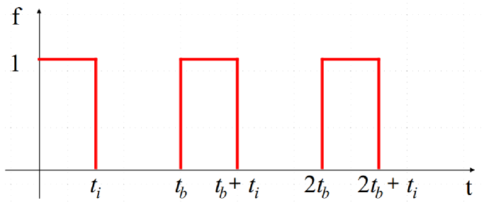
Figure 1: The function $f(t)$

Let us denote by $v_{1}$ and $v_{2}$ the temperatures in both areas, then the equation of thermal conduction for these areas has the form

$$\frac{\partial^{2}v_{1}}{\partial r^{2}}+\frac{1}{r}\frac{\partial v_{1}}{\partial r}-\frac{1}{\sigma_{1}}\frac{\partial v_{1}}{\partial t} = -\frac{A_{0}}{k_{1}}f(t),\,\,\,\,\,\,\,\,\,\,0<r<a;$$ (6)

$$\frac{\partial^{2}v_{2}}{\partial r^{2}}+\frac{1}{r}\frac{\partial v_{2}}{\partial r}-\frac{1}{\sigma_{2}}\frac{\partial v_{2}}{\partial t} = 0,\,\,\,\,\,\,\,\,\,\,\,\,\,\,\,\,\,\,\,\,\,\,\,\,\,\,\,\,\,\,\,\,\,\,\,\,\,\,\,\,r>a.$$ (7)

With the boundary conditions, that the temperature and the heat flow at the boundary between two media with different properties are continuous

$$v_{1}=v_{2},\,\,\,\,\,\,\,\,\,\,\mbox{and}\,\,\,\,\,\,\,\,\,\,\,\,\,\,\,k_{1}\frac{\partial v_{1}}{\partial r}=k_{2}\frac{\partial v_{2}}{\partial r}\,\,\,\,\,\mbox{at}\,\,\,\,\,r=a.$$ (8)

Let us solve these equations with the help of Laplace transformations ($t\Leftrightarrow p$). After the transformation ($\bar{v}_{1},\bar{v}_{2}$ and $\bar{f}$ denoting the conversed quantities) they take the form

$$\frac{\partial^{2}\bar{v}_{1}}{\partial r^{2}}+\frac{1}{r}\frac{\partial\bar{v}_{1}}{\partial r}-\frac{1}{\sigma_{1}}\frac{\partial\bar{v}_{1}}{\partial r} = -\frac{A_{0}}{k_{1}}\bar{f}(p),\,\,\,\,\,0<r<a;$$ (9)

$$\frac{\partial^{2}\bar{v}_{2}}{\partial r^{2}}+\frac{1}{r}\frac{\partial\bar{v}_{2}}{\partial r}-\frac{1}{\sigma_{2}}\frac{\partial\bar{v}_{2}}{\partial r} = 0,\,\,\,\,\,\,\,\,\,\,\,\,\,\,\,\,\,\,\,\,\,\,\,\,\,\,\,\,\,\,\,\,\,\,\,\,\,\,r>a;$$ (10)

$$\bar{v}_{1}=\bar{v}_{2}\,\,\,\,\,\,\,\,\,\,\mbox{and}\,\,\,\,\,\,\,\,\,\,\,\,\,\,k_{1}\frac{\partial\bar{v}_{1}}{\partial r}=k_{2}\frac{\partial\bar{v}_{2}}{\partial r}\,\,\,\,\,\,\,\,\,\,\mbox{at}\,\,\,\,\,\,\,\,\,\,r=a.$$ (11)

Here $\bar{f}(p)=\displaystyle\frac{1}{p}\frac{1-e^{-pt_{i}}}{1-e^{-pt_{b}}}$, and $p$ is the Laplace variable.

The solutions should be found from the requirements, that at $r=0$, $v_{1}$ has the finite value, and at $r\to\infty$ quantity $v_{2}$ is limited. The required solutions look like

$$\bar{v}_{1} = \frac{1}{p}\frac{\sigma_{1}A_{0}}{k_{1}}\left(1-\frac{k_{2}\sigma_{1}^{1/2}}{\Delta}K_{1}(a_{2}a)I_{0}(a_{1}r)\right)\bar{f}(p)=\bar{v}_{1}(p)\bar{f}(p)$$ (12)

$$\bar{v}_{2} = \frac{1}{p}\frac{\sigma_{1}A_{0}}{k_{1}}\frac{k_{1}\sigma_{2}^{1/2}}{\Delta}I_{1}(a_{1}a)K_{0}(a_{2}r)\bar{f}(p)=\bar{v}_{2}(p)\bar{f}(p)$$ (13)

where $I_{0}(x)$, $I_{1}(x)$, $K_{0}(x)$, $K_{1}(x)$ are the modified Bessel functions,

$$\Delta = k_{1}\sigma_{2}^{1/2}\left(I_{1}(a_{1}a)K_{0}(a_{2}a)+\frac{\sigma}{k}I_{0}(a_{1}a)K_{1}(a_{2}a)\right),$$ (14)

$$\sigma = \sqrt{\frac{\sigma_{1}}{\sigma_{2}}},\,\,\,\,\,\,k=\frac{k_{1}}{k_{2}},\,\,\,\,\,\,a_{1,2}=\sqrt{\frac{p}{\sigma_{1,2}}}.$$

Let us apply the inversion theorem [11] to $\bar{v}_{1}$

$$v_{1}(t)=\frac{1}{2\pi\imath}\frac{\sigma_{1}A_{0}}{k_{1}}\int_{\gamma-\imath\infty}^{\gamma+\imath\infty}\left(1-\frac{k_{2}\sigma_{1}^{1/2}}{\Delta}K_{1}(\mu_{2}a)I_{0}(\mu_{1}r)\right)\bar{f}(\lambda)\frac{e^{\lambda t}}{\lambda}d\lambda,$$ (15)

where $\gamma$ is to be so large that all singularities of $\bar{v}_{1}(\lambda)$ lie to the left of the line ($\gamma-\imath\infty,\gamma+\imath\infty$)(see Fig.2).

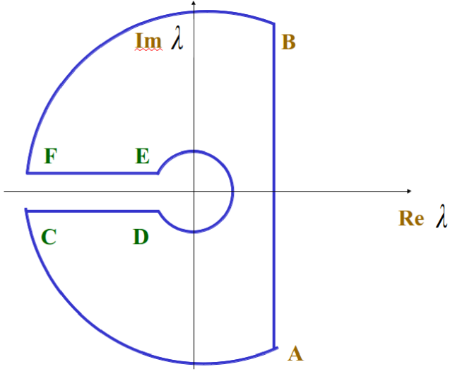
Figure 2: The contour of integration

In the relation (12) we have replaced $p$ with $\lambda$ to emphasize that in this relation we consider the behavior of the function $\bar{v}_{1}$, assuming it to be a function of the complex variable $\mu_{1,2}=\sqrt{\frac{\lambda}{\sigma_{1,2}}}$ .

The integrand in (15) has a point of branching at $\lambda=0$ and simple poles at $\lambda_{n_{0}}=\pm\imath\displaystyle\frac{2\pi n_{0}}{t_{b}}$, where $n_{0}=1,2,3...$. In this case we use a contour (see Fig. 2) with a cut along the negative real semiaxis so that $\bar{v}(\lambda)$ is a single-valued function $\lambda$ on a contour and outside it. The argument $\lambda$ on $EF$ is $\pi$, and on $CD$ the argument is $-\pi$.

Using the residue formula

$$\mathop{Res}\limits_{x=a}\frac{\phi(\lambda)}{\psi(\lambda)}=\frac{\phi(a)}{\psi^{\prime}(a)},\,\,\,\,\,\phi(a)\neq 0,\,\,\,\,\,\psi(a)=0,\,\,\,\,\,\psi^{\prime}(a)\neq 0,$$

we obtain

$$(v_{1})_{res}=\frac{\sigma_{1}t_{b}a_{0}}{\pi^{2}k_{1}}\sum_{n_{0}=1}^{\infty}\frac{\sin\frac{\pi n_{0}t_{b}}{t_{i}}}{n_{0}^{2}}\eta_{n_{0}}(r)\sin\left[\frac{2\pi n_{0}}{t_{b}}\left(t-\frac{t_{i}}{2}\right)+\epsilon_{n_{0}}(r)\right],$$ (16)

where functions $\eta_{n_{0}}(r)$ and $\epsilon_{n_{0}}(r)$ have the form

$$\eta_{n_{0}}(r)=\sqrt{Re^{2}(A+B)+Im^{2}(A-B)};\,\,\,\,\,\epsilon_{n_{0}}(r)=\arcsin\frac{A-B}{A+B},$$ (17)

$$A,B=1-\frac{\sigma}{k}\frac{I_{0}\left(N_{1}re^{\pm\imath\frac{\pi}{4}}\right)K_{1}\left(N_{2}ae^{\pm\imath\frac{\pi}{4}}\right)}{I_{1}\left(N_{1}ae^{\pm\imath\frac{\pi}{4}}\right)K_{0}\left(N_{2}ae^{\pm\imath\frac{\pi}{4}}\right)+\frac{\sigma}{k}I_{0}\left(N_{1}ae^{\pm\imath\frac{\pi}{4}}\right)K_{1}\left(N_{2}ae^{\pm\imath\frac{\pi}{4}}\right)},$$ (18)

$$N_{1,2}=\sqrt{\frac{2\pi n_{0}}{\sigma_{1,2}t_{b}}}.$$ (19)

Let us consider now the integral (15) (without the factor $\frac{1}{\lambda}$ or (12) without $\frac{1}{p}$) on the contour $ABFEDCA$ at a passage to the limit when the radius of the large circle $R$ tends to infinity, and the radius of the small one tends to zero. At $R\to\infty$ the integral over the arcs $BF$ and $CA$ tends to zero. As the radius of the small circle with the center at the origin of coordinates approaches zero, the integral on this circle also tends to zero. At $R\to\infty$ the integral over the $AB$ becomes equal to integral in Eq. (15). On the line $EF$ we assume $\lambda=\sigma_{1}u^{2}e^{\imath\pi}$, then the integral in (15) will be

$$2\int_{0}^{\infty}\frac{e^{-\sigma_{1}u^{2}t}}{u}\left[1-\frac{k_{2}\sigma_{1}^{1/2}}{\Delta}K_{1}\left(uae^{\imath\frac{\pi}{2}}\right)I_{0}\left(\sigma ure^{\imath\frac{\pi}{2}}\right)\right]\frac{1-e^{\sigma_{1}u^{2}t_{i}}}{1-e^{\sigma_{1}u^{2}t_{b}}}du$$

$$=\frac{2}{k_{1}\sigma_{2}^{1/2}}\imath\int_{0}^{\infty}\frac{e^{-\sigma_{1}u^{2}t}}{u}\frac{k_{2}\sigma_{1}^{1/2}}{u}\frac{J_{0}(ur)[J_{1}(\sigma ua)\phi-Y_{1}(\sigma ua)\psi]}{\phi^{2}+\psi^{2}}\frac{1-e^{\sigma_{1}u^{2}t_{i}}}{1-e^{\sigma_{1}u^{2}t_{b}}}du.$$ (20)

The integral over $CD$ gives an expression conjugate to (20), with the negative sign. Summarizing these results, we obtain for the integral

$$v_{1}^{\prime}(t)=\frac{1}{2\pi}\frac{A_{0}\sigma_{1}}{k_{1}}\frac{\sigma}{k}\int_{0}^{\infty}\frac{e^{-\frac{t}{\tau}x^{2}}}{x}\frac{J_{0}(x\frac{r}{a})[J_{1}(\sigma x)\phi-Y_{1}(\sigma x)\psi]}{\psi^{2}+\phi^{2}}\frac{1-e^{-\frac{t_{i}}{\tau}x^{2}}}{1-e^{-\frac{t_{b}}{\tau}x^{2}}}dx,$$ (21)

where parameter $\tau$, functions $\phi$ and $\psi$ have the form

$$\phi = J_{1}(x)Y_{0}(\sigma x)-\frac{\sigma}{k}J_{0}(x)Y_{1}(\sigma x),$$ (22)

$$\psi = J_{1}(x)Y_{0}(\sigma x)-\frac{\sigma}{k}J_{0}(x)J_{1}(\sigma x),\,\,\,\,\,\,\,\,\,\,\tau=\frac{a^{2}}{\sigma_{1}}.$$

In the derivation of Eq. (21) the following relations have been used [11]:

$$I_{1}(\pm\imath z) = \pm\imath J_{1}(z),\,\,\,\,\,\,\,\,\,\,I_{0}(\pm\imath z)=J_{0}(z),$$ (23)

$$K_{0}(\pm\imath z) = \mp\frac{\imath\pi}{2}\left[J_{0}(z)\mp\imath Y_{0}(z)\right],\,\,\,\,\,K_{1}(\pm\imath z)=-\frac{\pi}{2}\left[J_{1}(z)\mp\imath Y_{1}(z)\right].$$

The expression in square brackets in the numerator of Eq. (21) is equal to $\left[...\right]=\frac{2}{\pi\sigma x}J_{1}(x)$, where the formula

$$J_{0}(z)Y_{1}(z)-J_{1}(z)Y_{0}(z)=-\frac{2}{\pi z}$$

(see, e.g.,[12]) is used. Then we arrive at the expression

$$v_{1}^{\prime}(t)=\frac{4}{\pi^{2}k}\frac{A_{0}\sigma_{1}}{k_{1}}\int_{0}^{\infty}\frac{e^{-\frac{t}{\tau}x^{2}}}{x^{2}}\frac{J_{1}(x)J_{0}\left(\frac{x}{a}\right)}{\phi^{2}+\psi^{2}}\frac{1-e^{-\frac{t_{i}}{\tau}x^{2}}}{1-e^{-\frac{t_{b}}{\tau}x^{2}}}dx.$$ (24)

Using the formula [10]

$$\frac{\bar{v}_{1}^{\prime}(p)}{p}\Leftrightarrow\int_{0}^{t}\bar{v}_{1}^{\prime}(\tau)d\tau,$$

we finally get

$$(v_{1}(t))_{contour}=\frac{4A_{0}a^{2}}{\pi^{2}kk_{1}}\int_{0}^{\infty}\frac{1-e^{-\frac{t}{\tau}x^{2}}}{x^{4}}\frac{1-e^{-\frac{t_{i}}{\tau}x^{2}}}{1-e^{-\frac{t_{b}}{\tau}x^{2}}}\frac{J_{1}(x)J_{0}\left(x\frac{r}{a}\right)}{\phi^{2}+\psi^{2}}dx.$$ (25)

With Eqs. (12) and (16) taken into account the general expression for $v(t)=(v(t))_{contour}+(v(t))_{res}$ will take the form

$$v_{1}(t) = \frac{4A_{0}a^{2}}{\pi^{2}kk_{1}}\int_{0}^{\infty}\frac{1-e^{-\frac{t}{\tau}x^{2}}}{x^{4}}\frac{1-e^{-\frac{t_{i}}{\tau}x^{2}}}{1-e^{-\frac{t_{b}}{\tau}x^{2}}}\frac{J_{1}(x)J_{0}\left(x\frac{r}{a}\right)}{\phi^{2}+\psi^{2}}dx$$

$$+ \frac{\sigma_{1}t_{b}a_{0}}{\pi^{2}k_{1}}\sum_{n_{0}=1}^{\infty}\frac{\sin\frac{\pi n_{0}t_{b}}{t_{i}}}{n_{0}^{2}}\eta_{n_{0}}(r)\sin\left[\frac{2\pi n_{0}}{t_{b}}\left(t-\frac{t_{i}}{2}\right)+\epsilon_{n_{0}}(r)\right].$$

The first term $(v_{1})_{res}$ obtained from the residues at the poles $\lambda_{n_{0}}=\pm\imath\frac{2\pi n_{0}}{t_{b}}$, $n_{0}=1,2,3,...$ represents a part of the solution relevant to a stationary state. It is easy to show, that at small times

$$(v_{1}(t))_{contour}=\frac{t_{i}}{t_{b}}\frac{\sigma_{1}A_{0}}{k_{1}}t,$$ (27)

and at large times

$$(v_{1}(t))_{contour}=\frac{t_{i}}{t_{b}}\frac{a^{2}A_{0}}{2k_{1}}\ln\frac{4\sigma_{2}t}{Ca^{2}},$$ (28)

where $C=1.7811={e}^{\gamma}$, $\gamma=0.5772$ is the Euler constant.

In the same way, one can obtain from (7)

$$v_{2}(t)\!\! = \!\!\frac{2A_{0}a^{2}}{\pi k_{1}}\int_{0}^{\infty}\frac{1-e^{-\frac{t}{\tau}x^{2}}}{x^{4}}\frac{1-e^{-\frac{t_{i}}{\tau}x^{2}}}{1-e^{-\frac{t_{b}}{\tau}x^{2}}}\frac{J_{1}(x)\left[J_{0}\left(\sigma x\frac{r}{a}\right)\phi-Y_{0}\left(\sigma x\frac{r}{a}\right)\psi\right]}{\phi^{2}+\psi^{2}}dx\qquad\;\;\;$$ (29)

$$\qquad\quad\;+\;\;\frac{\sigma_{1}t_{b}a_{0}}{\pi^{2}k_{1}}\sum_{n_{0}=1}^{\infty}\frac{\sin\frac{\pi n_{0}t_{b}}{t_{i}}}{n_{0}^{2}}\xi_{n_{0}}(r)\sin\left[\frac{2\pi n_{0}}{t_{b}}\left(t-\frac{t_{i}}{2}\right)+\zeta_{n_{0}}(r)\right],$$

where functions $\xi_{n_{0}}(r)$ and $\zeta_{n_{0}}(r)$ have the form

$$\xi_{n_{0}}(r)=\sqrt{Re^{2}(a+b)+Im^{2}(a-b)};\,\,\,\,\,\zeta_{n_{0}}(r)=\arcsin\frac{Im(a-b)}{Re(a+b)},$$ (30)

$$a,b=\frac{I_{1}\left(N_{1}ae^{\pm\imath\frac{\pi}{4}}\right)K_{0}\left(N_{2}re^{\pm\imath\frac{\pi}{4}}\right)}{I_{2}\left(N_{1}ae^{\pm\imath\frac{\pi}{4}}\right)K_{0}\left(N_{2}ae^{\pm\imath\frac{\pi}{4}}\right)+\frac{\sigma}{k}I_{0}\left(N_{1}ae^{\pm\imath\frac{\pi}{4}}\right)K_{1}\left(N_{2}ae^{\pm\imath\frac{\pi}{4}}\right)},$$ (31)

and $N_{1,2}$ is given by (19).

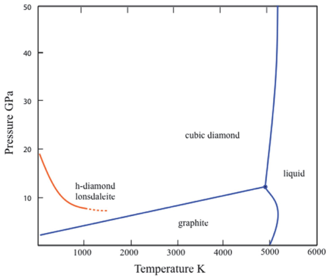
Figure 3: Phase diagram of graphite

3 Conclusion

It should be taken into account that for the temperature available in Yerevan Physics Institute accelerators temperature ($T\ll 10000^{\circ}K$) the role of electronic terms can be neglected; and the elastic pressure comparable with the thermal one or exceeds it. Therefore, for an estimate of the values of pressures and temperatures, it is possible to restrict ourselves to the thermal terms only ($T\gg T_{0}$, $T_{0}$ being the room temperature)

$$P=H\frac{E}{V},\,\,\,\,\,\,\,\,\,\,E=3NkT,$$ (32)

where $P$ is the pressure, $H$ is the Hrunaisen coefficient, which we take be equal to 2 for graphite, $V$ is the graphite volume, $N$ is the number of atoms in the volume $V$, $k=1.38\times 10^{-23}$ J/K is the Boltzmann constant, $T$ is the temperature. Using Eqs. (25) – (32) we find, that the temperature $T=3000$^∘ C corresponds to pressure $P=27\,$ GPa in the case of sand environment, and the temperature $T=1000^{\circ}$ C corresponds to $P=9$ GPa in the case of steel environment

These parameters $(3000^{\circ}$ C, 27 GPa), $(1000^{\circ}$ C, 9 GPa) in the ($P,T$) diagram figure a point in the field of stability of diamond (see Fig.3). We shall note also, that direct equations of state $P=9.1\times(10^{-3}T)$ GPa in the ($P,T$) diagram lays in the field of stability of diamond which is higher than the curve of equilibrium diamond - graphite.

4 Acknowlegments

Authors thank to Dr. A.S. Ayriyan for useful discussion and remarks. For KBO and NShI this work was supported by the Science Committee of the Ministry of Science and Education of the Republic of Armenia (grant number 13-1C080). KBO thanks LIT JINR for hospitality and support during his visit.

References

[1]
Batsanov S.S., Demidov B.A. and Rudakov L.I.
Use of a high-current relativistic electron beam for structural and chemical transformations .
Pisma v ZhETF 1979 30, pp. 611-613; JETP Lett. 1979 30, 575–577
[2] Batsanov, S.S., Demidov, B.A., Ivkin, M.V., Kopaneva, L.I., Lazareva, E.V., Martynov, A.I., Petrov, V.A.
Carbide synthesis and phase transition of boron nitride under the influence of high current density relativistic electron beam.
Izvestiya Akademii Nauk SSSR, Neorganicheskie Materialy 1990, 26, N 10, pp. 2100–2102;
Inorganic Materials 1990, 26, N 10, pp. 2100–2102
[3] Amatuni A. Ts.
Nonlinear effects in plasma wake field acceleration (PWFA)
in Proc. of Workshop on Role of Plasmas in Accelerators
1989, Tsukuba, Ibaraki: National Lab. for High Energy Physics, pp. 81-97
[4] Zel’dovich Ya.B. and Raiser Yu.P.
Physics of shock waves and high-temperature hydrodynamic phenomena. N.-Y.: Academic Press, V 1, 1966. 464 p.; V. 2, 1967. 451 p.
[5] Altshuller L.B., Krupnikov K.K., Brazhnik M.I.,
Dynamic compressibility of metals under pressures
from 400,000 to 4,000,000 atmospheres.
Sov. Phys. JETP, 1958, 7, pp. 614-619