The giant low-density lipoproteins (LDL) accumulation in the multi-layer artery wall model

Abstract

The mathematical, four-layer model of the LDL transport across the arterial wall including the sensitivity of the transport coefficients to the wall shear stress (WSS) is studied. In that model the advection–diffusion equations in porous media are used to determine the LDL concentration profiles in each layer of the arterial wall. We demonstrate the effect of the giant accumulation of the LDL in the intima layer. This property turns out to be an interplay between the layered structure of the arterial wall and WSS sensitivity of the endothelium. Interestingly, we also show that the single-layer models with the same WSS sensitivity mechanism and corresponding parameters, obscure the accumulation phenomenon, which predicts the one order of magnitude larger LDL concentration.

The paper is supplemented by the repository with source code of the model [1].

1 Introduction

Sudden cardiac death refers to estimated 4-5 million people per year [2] and it is one of the major causes of mortality in the adult population. Almost 80 % of all sudden cardiac deaths is connected with the myocardial ischemia caused by the atherosclerosis and more specifically by coronary artery disease[3, 4]. For these reasons the pathogenesis of atherosclerosis and evolution of atherosclerotic plaque are extensively studied all over the world.

It is assumed that the development of atherogenesis is associated with the abnormally high accumulation of the low-density lipoproteins in the intima [5]. The LDL is responsible for the transport of cholesterol from the liver to the all tissues of the human body. Due to its putative role as an atherosclerosis precursor the issue of the transport of the LDL molecules in the arterial walls of the circulatory system and the factors influencing this transport are widely studied.

One of such factors is the wall shear stress acting on the wall of the vessel, and directly on the endothelial cells. It is well accepted that the occurrence of atherosclerosis is related to the exposure of the endothelial cells to the low or oscillatory WSS [6].

The impact of the wall shear stress on the LDL transport has recently been a subject of various computational research. In order to properly capture the processes occurring in the blood vessel wall, it is necessary to create mathematical description of the complicated artery wall structure. The class of so called ’multi-layer’ models turned out to reasonably well capture the properties of the arterial wall. An example is the four-layer model proposed by Ai and Vafai in [7].

In this work we study the properties of the arterial wall described as a four-layer medium and, at the same time, sensitive to WSS value.

It is almost impossible to precisely obtain the transport properties corresponding to the different layers of the wall during experimental study. Therefore we will use two sets of estimated parameter values reported in [7, 8]. The essential difference between them is in the internal elastic lamina (IEL) properties.

We will show that in the multi-layer models the LDL accumulation between the layers with the low LDL permeability is possible. Depending on the used set of parameters of the model, LDL concentration can be up to twenty times larger then it was expected at the based on previously reported results, e.g. [9].

This paper is structured as follows. Section 2 describes structure of the arterial wall with focus on the layers used in the modeling. Section 3 reviews known arterial wall models, in particular the detailed description of the four-layer model, developed by Ai and Vafai in [7]. In Section 4 we summarize the details of the wall shear stress impact on the LDL transport, used in modeling. Section 5 presents parameters and implementation of our computer simulations. In Section 6 we discuss the results of the simulations focusing on the giant LDL accumulation in the intima. Finally in Section 7 we will draw conclusions.

2 Structure of the arterial wall

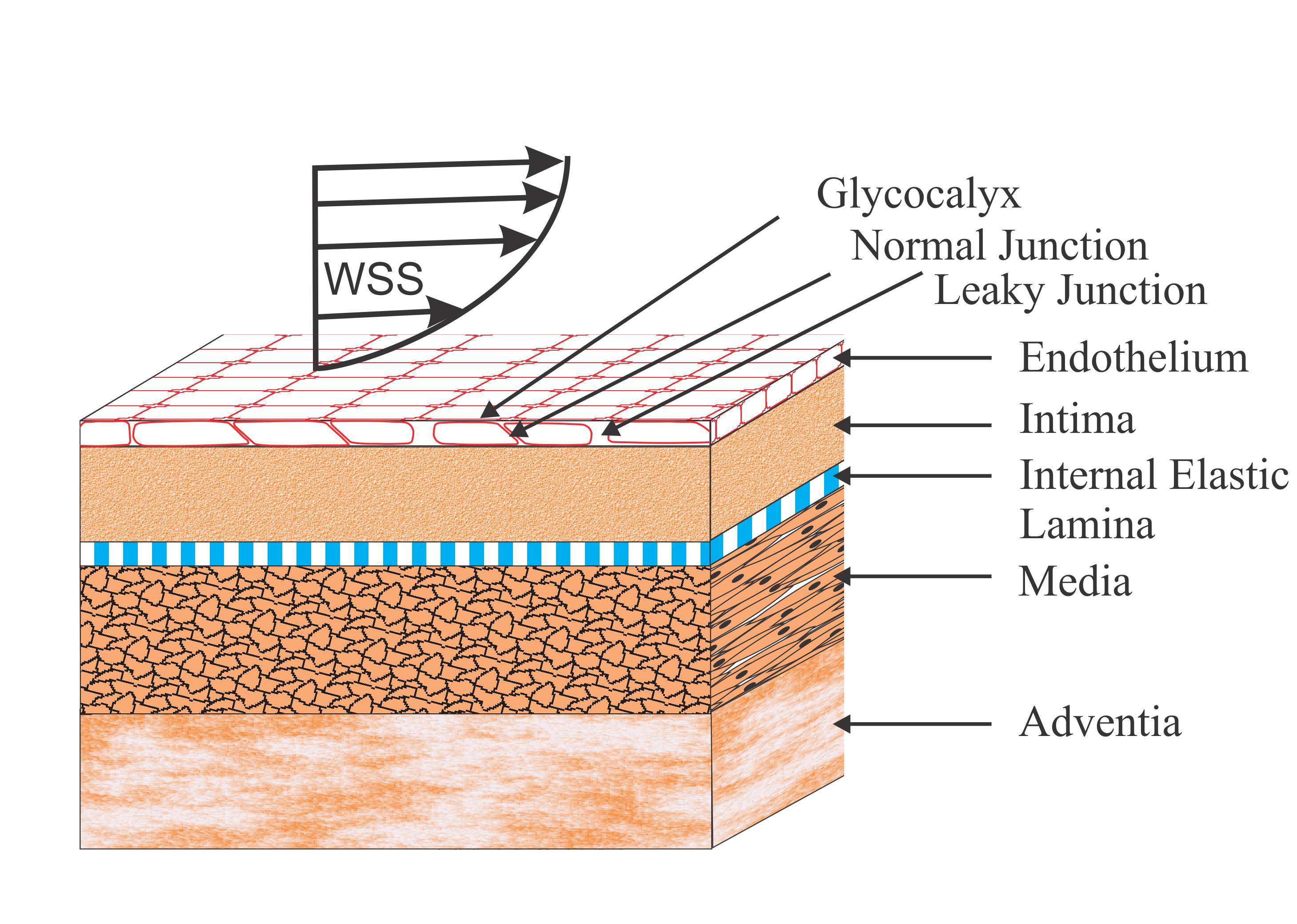
Figure 1: Section of artery together with a schematic indication of WSS profile near the wall.

A typical large blood vessel has a layered structure, schematically shown in the Figure 1. It is composed of the six layers. The glycocalyx is the first layer, which is in direct contact with blood. Its thickness ranges from about $30$ to $100nm$ (averaged thickness is $60nm$) [10]. It is a carbohydrate layer that covers the single layer of endothelial cells and the entrances of intercellular junctions [11].

Endothelium is the second $2\mu m$ thick layer. It is a major barrier in the LDL migration outside the lumen and at the same time has the highest sensitivity to the conditions in the lumen. Endothelium changes its transport properties depending on WSS value [10]. The results contained in this paper are in large extend a consequence of this sensitivity.

Directly behind the endothelium lies $10\mu m$ thick intima. This is a cushion layer made of connective tissue which may contain smooth muscle cells and few fibroblasts. This layer is relatively easily penetrable by both plasma and macromolecules [11].

Between the intima and the media is another membrane - internal elastic lamina, constructed of impermeable connective tissue with fenestral pores. Its thickness is assumed to be $2\mu m$. This membrane is a significant barrier to the LDL lipoproteins. In this work we will demonstrate that under certain conditions, this might be a cause for the LDL accumulation [11].

Media, the thickest layer ($200\mu m$), is made up of the alternating layers of the smooth muscle cells and elastic connective tissue. In media the absorption of the LDL particles takes place[11].

Media is surrounded by the adventitia, which consists of collagen fibres attaching the arterial wall to surrounding flabby connective tissue.

3 Modeling macromolecules transport in the arterial wall

Realistic modeling of WSS effects on the LDL transport is still a big challenge. Models including more details of the wall structure obviously tent to be more difficult to implement and more demanding computationally. At the same time they have more free parameters which need to be precisely measured. On the other hand oversimplified models might overlook some important properties. Below we briefly review commonly used approaches.

Prosi et al. [12] divided vessel wall modeling into three groups according to its degree of complexity. The simplest model used i.a. in [13, 14] is the wall-free model. It treats the arterial wall as a simplified boundary condition. The advantage of this approach is its simplicity, but that model does not allow to obtain information relating to the transport in the arterial wall, but only in the lumen [9].

More complicated, and thus more realistic is the lumen-wall model, in which the transport of macromolecules is considered both in the lumen and in the wall. This model was proposed by Moore and Ethier [15]. Olgac et al. used this model in [9], where the dependence of the LDL transport properties on WSS was proposed. This model treats the arterial wall as a homogeneous porous media. Hence, it is possible to observe the macromolecules transport in the lumen and in the artery wall, what is the main advantage of this approach. Despite of that, this model is relatively simple in comparison to the last branch of transport models, which is a multi-layer model.

Multi-layer model takes into account the internal structure of the blood vessel wall, thus better reflects the properties of the actual arterial wall. On the other hand this advantage causes the complexity increase. One of the multi-layer models is the four-layer model proposed by Ai and Vafai in [7]. In this model, the arterial wall is represented by the four layers: endothelium, intima, IEL and media. Detailed description of this model is presented in the next section.

3.1 Four-layer model

Ai and Vafai in [7] developed an artery model taking into account the layered structure of the blood vessel. Endothelium, intima, IEL and media are the layers that are covered in this model. They are shown in the Figure 1. Due to its very small thickness, the impact of the glycocalyx is neglected. Adventitia is taken into account as a boundary condition at the opposite side of the system.

Endothelium and IEL are semi-permeable membranes and filtration theory is applied to model them, while the intima and media can be modeled as a porous media. The phenomenon of the osmosis for semi-permeable membranes can be ignored, because the gradients of the LDL are too small to influence the hydraulic processes [11]. In this case, the equations for transport through the membranes are effectively the same as those for transport through the porous media, but with the different coefficients for each layer. For this reason, the layers are all treated as a macroscopically homogeneous porous media and mathematically modeled using the volume averaged porous media equations, with the Staverman filtration and osmotic reflection coefficients. These coefficients allow to account for selective permeability of each porous layer to the LDL macromolecules.

Finally, a description of the LDL transport in each layer of the arterial wall is reduced to the following equations for the hydraulic and filtration processes:

$$\frac{\rho}{\delta}\frac{\partial\vec{u}}{\partial t}+\frac{\mu_{eff}}{K}\vec{u} = -\nabla p+\mu_{eff}\nabla^{2}\vec{u}$$ (1)

$$\frac{\partial c}{\partial t}+(1-\sigma)\vec{u}\cdot\nabla c = D_{eff}\nabla^{2}c-kc$$ (2)

where $\rho$ is the fluid density, $\delta$ is the porosity, $\mu_{eff}$ is the medium effective dynamic viscosity for the LDL, $K$ is the permeability, $p$ is the pressure, $\sigma$ is the reflection coefficient, $\vec{u}$ is the hydraulic velocity of the solvent penetration and $D_{eff}$ is the diffusivity. The model assumes first order decay of the LDL in media with the reaction rate coefficient $k$.

Equation 1 in practice, can be replaced by the adiabatic approximation in which the filtration velocity is determined immediately and given by:

$$\vec{u} = -\frac{K}{\mu_{eff}}\nabla p$$ (3)

The Equation 3 has a similar form to the (continuous) Ohm’s law for electrical circuits: $\frac{K}{\mu_{eff}}$ is the equivalent of conductance, $\Delta p$ voltage, and $\vec{u}$ current. For this reason, to the description of the connected layers, the analogy to parallel and serial connections can be applied. Subsequent layers are treated as resistors connected in series and the individual normal and leaky junctions in the endothelial layer are treated as parallel resistors.

3.2 One-dimensional approximation

System under consideration has very diverse scales. This allows to express the hypothesis that major simplifications will not substantially change the results of calculations. First, the wall is thin compared to the length or circumference of the vessel. For example, in the case of the coronary arteries, circuit is in range of $10^{4}\mu m$ and substantial thickness of the arterial wall does not exceed $10^{2}\mu m$. In addition, permeation processes are dominated by the pressure forced filtration and predominantly occurs in the radial direction. Thus the process of the LDL transport in the artery takes place essentially in the this direction. As a result, our modeling can be reduced to the one spatial dimension.

In the literature, a comparison of the two-and three-dimensional models with the one dimensional ones confirms this assumption [8, 11, 16]. Additionally, we have compared our one-dimensional results with three-dimensional simulation done by Olgac et al. [9]. The results are discussed in the Section 6.

4 Effect of WSS on LDL transport in the arterial wall

It has been observed, that atherosclerotic lesions are formed in the specific areas of the circulatory system: the outer wall of bifurcations and the inner wall of curvatures. A common feature of these regions is the presence of disturbed flow [6, 17]. That tendency was first noticed by Caro et al. [18]. Whereas later it has been confirmed in several different ways: by using the computational fluid dynamic simulations [19, 20, 21], in-vivo studies in animals [22, 23, 24] and in vivo investigations in humans thanks combination of the advanced medical imaging techniques and computer simulations [25, 26, 27].

For simple blood vessels the WSS amplitude ranges from 1.5-7 Pa and has a positive time average [6, 28, 29, 30]. Such physiological level of the shear stress appears to play a protective role for the functional integrity of the endothelial cells [31]. However, in the areas where the disturbed blood flow occurs, the low WSS is observed. This WSS is defined by low amplitude, on average 0.02-1.2 Pa [6, 25, 28, 30, 32]. In the case of low WSS increased endothelial cell turnover rate is observed [25].

4.1 WSS dependent mechanism of the LDL transport by the endothelium

The mechanism of the macromolecules transport in the arterial wall is in large part defined by the endothelium. This layer causes increased hydraulic and mass transfer resistance. It is related to the small pore size. Therefore, factors which cause an increase in the effective pore size have a significant impact on the flow in the endothelium, and thus in the entire wall.

The endothelium cells are connected to each other by the intracellular junctions. These junctions can be normal or leaky. Therefore, in this layer three pathways can be distinguished: vesicular pathway, normal junctions, and leaky junctions. The vesicular pathway is responsible only for ($\sim 9\%$) of the LDL transport[9] and is not taken into the account in this paper.

Intercellular junctions would not normally allow any significant passage of the LDL even through breaks in the normal junction, because the wide part of the cleft is expected to be of the order of LDL molecule size. The average radius of the normal junction is $5.5nm$, which is smaller than the radius of the LDL molecule ($r_{m}=11nm$). The large, leaky pores are associated with cells that are in the process of cell turnover: either cell division (mitosis) or cell death (apoptosis). The cause of the leaky junctions formation in these cells is the weakening of the junctions during the process of division or sloughed off this cells by the healthy neighbors [5].

Therefor the process consists of the flux of the solvent through normal and leaky junctions [9] with velocity which has to be calculated in the model. Then, this velocity drives the passage of LDL molecules through the leaky junctions. The key role in this scheme, plays a fraction of leaky junctions $\phi$ in the wall and its dependence on WSS.

It turns out that processes of apoptosis and mitosis are affected by wall shear stress. Several studies have shown that a reduction in the rate of blood flow or shear stress induces an increase in the rate of endothelial cell apoptosis, whereas an increase in shear stress exerts the opposite effect [31, 5].

The fraction $\phi$ is defined as the ratio of the area of leaky cells to the area of all cells [33]. This is shown schematically in the Figure 2. According to this:

$$\phi=\frac{R_{cell}^{2}}{\xi^{2}}$$ (4)

where $R_{cell}$ is the radius of the endothelial cell taken as $15\mu m$ and $\xi$ is radius of periodic circular unit [34].

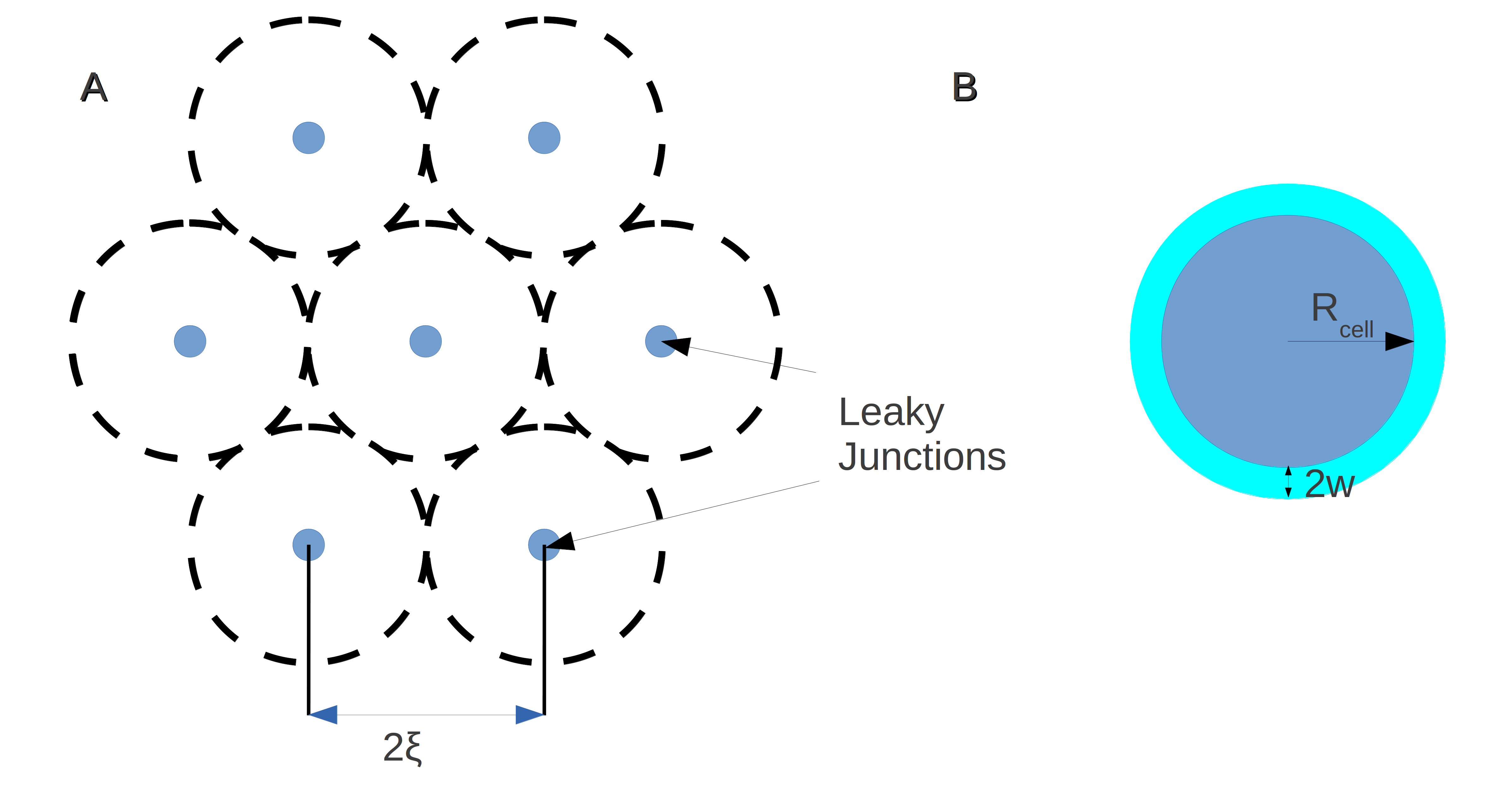
Figure 2: illustration of randomly distributed leaky cells. (A) A leaky cell represented by blue circle is present at the center of each periodic circular unit of radius $\xi$ represented by dashed lines. (B) Leaky cell of radius $R_{cell}$ with leaky junction of half-width $w=10nm$.

Olgac et al. in [9] developed a model which allows to calculate the fraction of leaky junctions. For self integrity of the paper we will shortly review details of this approach.

The procedure was done in four steps, which we will summarize below.

In the first step the relation of the shape index (SI):

$$SI=\frac{4\pi\times area}{(perimeter)^{2}}$$ (5)

and WSS was established. Based on experimental results from [35, 36, 37] it was found that:

$$SI=0.380\times e^{0.79\cdot\mathrm{WSS}}+0.225\times e^{0.043\cdot\mathrm{WSS}}$$ (6)

In the second step the shape index was associated with the number of mitotic cells per area of $0.64mm^{2}$. The function fitted by Olgac et al.[9] to the data from[38] takes the following form:

$$N_{MC}=0.003797\times e^{14.75\cdot SI}$$ (7)

The third step was to get the ratio of leaky cells associated with mitotic cells to all mitotic cells. On that basis of the work [39] Olgac et al. derived the correlation of the number of mitotic cells with the number of all leaky junctions per area of $0.64mm^{2}$. They assumed that the number of leaky cells correlated with nonmitotic cells is independent on WSS. This relation is the following:

$$N_{LC}=0.307+0.805\times N_{MC}$$ (8)

In the last step, knowing the number of leaky cells in a given area (in this case $0.64mm^{2}$) fraction of leaky junctions was determined to be:

$$\phi=\frac{N_{LC}\times\pi R_{cell}^{2}}{6.4\times 10^{-7}}$$ (9)

The fraction of leaky junctions determine transport properties of the endothelium. Since in the endothelium is modeled as a medium with given diffusion $D$, reflection coefficient $\sigma$ and permeability $K$ we need the quantitative dependence of those parameters on $\phi$.

The LDL molecule diffuses in cylindrical pores (effectively treated as slits of width $2w$), therefore its diffusion coefficient can be approximated by [8]:

$$D_{end}=D_{lj}=D_{lumen}(1-\alpha_{lj})F(\alpha_{lj})\frac{4w}{R_{cell}}\phi$$ (10)

where $w$ is half width of leaky junctions equal $14nm$ (see Figure 2). $\alpha_{lj}$ is the ratio of $r_{m}$ to $w$ and $r_{m}$ radius of LDL molecule equal $11nm$. $(1-\alpha_{lj})$ is the partition coefficient, which is the ratio of the pore area available for solute transport to the total pore area [40]:

$$\alpha_{lj}=\frac{r_{m}}{w}$$ (11)

F is a hindrance factor for diffusion in a pore, given by Curry [40]:

$$F(\alpha_{lj})=(1-1.004\alpha_{lj}+0.418\alpha_{lj}^{3}-0.169\alpha_{lj}^{5})$$ (12)

Applying electric analogue, the endothelium permeability $K_{end}$ can be expressed as a sum of permeabilities of parallel pathways:

$$K_{end}=K_{lj}+K_{nj}$$ (13)

The permeability of the leaky junctions $K_{lj}$ is dependent on the fraction of leaky junctions $\phi$ and may be determined using formula for the permeability of a slit of width $2w$ multiplied by area fraction of a leaky junctions:

$$K_{lj}=\frac{w^{2}}{3}\frac{4w\phi}{R_{cell}}$$ (14)

WSS does not affect the normal junctions, so $K_{nj}$ is a constant. Therefore, it can be determined by using known data for $K_{end}(\phi=5\times 10^{-4})=3.22\times 10^{-15}mm^{2}$[8], thus:

$$K_{nj}=K_{end}(\phi=5\times 10^{-4})-K_{lj}(\phi=5\times 10^{-4})$$ (15)

Reflection coefficients for LDL transport are different for normal and leaky junctions. Normal junctions are impermeable for LDL, so the reflection coefficient $\sigma_{nj}=1$. Expression for the overall reflection coefficient of the endothelium can be calculated from $\sigma$ for each of the individual pathways from heteroporous model [41, 42, 43]. Similarly to (13) we have:

$${K_{end}}\sigma_{end}=K_{lj}\sigma_{lj}+K_{nj}\sigma_{nj}$$ (16)

thus:

$$\sigma_{end}=1-\frac{(1-\sigma_{lj})K_{lj}}{K_{nj}+K_{lj}},$$ (17)

where

$$\sigma_{lj}=1-W=1-(1-\frac{3}{2}\alpha_{lj}^{2}+\frac{1}{2}\alpha_{lj}^{3})(1-\frac{1}{3}\alpha_{lj}^{2})$$ (18)

and W is overall hindrance factor for convection[44].

Olgac et al. have applied empirical relations: (6,7,8,9) for construction of the realistic model comprising the effect of WSS on LDL transport. We will supplement this approach by taking into the account the fine structure of the artery wall.

5 Four-layer model with WSS sensitivity

In this work, we show properties of four-layer arterial wall model, which includes the impact of WSS on the transport properties given by the equations (6-9). Our computer simulation solves equation (2) in one-dimension, i.e.:

$$\frac{\partial c}{\partial t} = -(1-\sigma)u\cdot\frac{\partial c}{\partial x}+D_{eff}\frac{\partial^{2}c}{\partial x^{2}}-kc$$ (19)

with constant filtration velocity calculated from equation (3). The equation (19) is valid for coefficients $\sigma,D_{eff}$ independent on space, therefore it is true in each layer separately. At interfaces between layers the flux continuity condition must be fulfilled [11]:

$$\left.\left[(1-\sigma)\vec{u}c-D\frac{\partial c}{\partial x}\right]\right|_{+}=\left.\left[(1-\sigma)\vec{u}c-D\frac{\partial c}{\partial x}\right]\right|_{-}$$ (20)

where $+$ and $-$ particles flux at the the left and right side of the boundary, respectively.

We solve the equation (19) with imposed conditions (20) using the finite difference method. Matrix of the linear system, generated by the discretization procedure is sparse, band and symmetrical. We use package sparse from the Python SciPy library for the efficient handling and solving our equations. The details of the implementation as well as the full source code can be found on git repository [1].

Results in this work, are based on two sets of transport properties in the artery: Ai and Vafai (2006) [7] presented in the Table 1 (4LA) and Chang and Vafai (2012) [8] presented in the Table 2 (4LC).

Names	Endothelium	Intima	IEL	Media
Thickness L, $\mu m$	$2.0$	$10.0$	$2.0$	$200.0$
Diffusivity D, $mm^{2}/s$	$D(\mathrm{WSS})$	$5.4\times 10^{-6}$	$3.18\times 10^{-9}$	$5\times 10^{-8}$
Reflection coefficient $\sigma_{1}$	$\sigma_{1}(\mathrm{WSS})$	$0.8272$	$0.9827$	$0.8836$
Reaction rate coefficient k, $1/s$	$0$	$0$	$0$	$3.197\times 10^{-4}$
Permeability K, $mm^{2}$	$K(\mathrm{WSS})$	$2.0\times 10^{-10}$	$4.392\times 10^{-13}$	$2\times 10^{-12}$
Dynamic viscosity $\mu$, $g/(mm\cdot s)$	$0.72\times 10^{-3}$	$0.72\times 10^{-3}$	$0.72\times 10^{-3}$	$0.72\times 10^{-3}$

Table 1: Physiological parameters used in the numerical simulation from Ai and Vafai publication (2006)[7] (4LA). Parameters depending on the WSS are marked by (WSS).

Names	Endothelium	Intima	IEL	Media
Thickness L, $\mu m$	$2.0$	$10.0$	$2.0$	$200.0$
Diffusivity D, $mm^{2}/s$	$D(\mathrm{WSS})$	$5.0\times 10^{-6}$	$3.18\times 10^{-9}$	$5\times 10^{-8}$
Reflection coefficient $\sigma_{1}$	$\sigma_{1}(\mathrm{WSS})$	$0.8292$	$0.8295$	$0.8660$
Reaction rate coefficient k, $1/s$	$0$	$0$	$0$	$1.4\times 10^{-4}$
Permeability K, $mm^{2}$	$K(\mathrm{WSS})$	$2.2\times 10^{-10}$	$3.18\times 10^{-13}$	$2\times 10^{-12}$
Dynamic viscosity $\mu$, $g/(mm\cdot s)$	$0.72\times 10^{-3}$	$0.72\times 10^{-3}$	$0.72\times 10^{-3}$	$0.72\times 10^{-3}$

Table 2: Physiological parameters used in the numerical simulation from Chung and Vafai (2012) publication [8] (4LC). Parameters depending on the WSS are marked by (WSS).

Additionally, we will also present two-layer model equivalent to that from Olgac et al. [9]. In that case the parameters are summarized in Table 3.

Names	Endothelium	Wall
Thickness L, $\mu m$	$2.0$	$338.0$
Diffusivity D, $mm^{2}/s$	$D(\mathrm{WSS})$	$8.0\times 10^{-7}$
Reflection coefficient $\sigma_{1}$	$\sigma_{1}(\mathrm{WSS})$	$0.8514$
Reaction rate coefficient k, $1/s$	$0$	$3.0\times 10^{-4}$
Permeability K, $mm^{2}$	$K(\mathrm{WSS})$	$1.2\times 10^{-12}$
Dynamic viscosity $\mu$, $g/(mm\cdot s)$	$0.72\times 10^{-3}$	$0.72\times 10^{-3}$

Table 3: Physiological parameters used in the numerical simulation for two-layer model from Olgac et al. (2006) publication [9]. Parameters depending on the WSS are marked by (WSS).

6 Results

We solve numerically the equation (19) with Dirichlet boundary conditions: $c(0)=1.0$ and $c(214)=0$. Note that for clarity we use $\mu m$ as $x$ scale in the numerical algorithm. The value of the left boundary mimics the concentration of the LDL in the lumen, therefore due to linearity of the transport equation we might treat values of $c$ inside the arterial wall as relative concentrations to the lumen LDL level. The right boundary is absorbing, however replacing it with reflecting boundary does not visibly affect values of $c$ in the $x\in(0,50)$.

The filtration velocity is obtained from (3) with effective permeability of the system calculated from the circuit analogue (see source code [1]). The transmural pressure driving the flow in this paper is always taken to be $70\mathrm{mmHg}$.

6.1 Four-layer model for high WSS

In the first place our simulations are compared with the results reported in the literature. Such comparison has been made for two mentioned sets of parameters. In both cases, the simulations were performed for WSS equal $2.2Pa$. The WSS around $2Pa$, is a typical physiological value in arteries in free segments without any obstructions or bifurcations. In the Figure 3 comparison of the results for the parameters (4LA) with the data from [7] is shown.

An analysis of the graph shows the difference between the obtained results marked by blue dashed line, and the results from the publication marked by red crosses. These results slightly differ in the endothelium concentration profile. To check the reason of this difference, the parameters, which in our case depend on WSS were compared with the one used in the [7]. That comparison shows clearly that this difference is caused by the difference between the diffusion coefficient obtained from the relation $D(\mathrm{WSS})$ in Equation 10, and found in the publication [7]. This is confirmed by the orange continuous line, which shows results of our simulation with constant $D(\mathrm{WSS})=8.15\times 10^{-11}mm^{2}/s$ coinciding with the work of Ai and Vafai. An important observation is also that the choice of the diffusion coefficient does not influence the shape of the profile in intima, IEL and media layers.

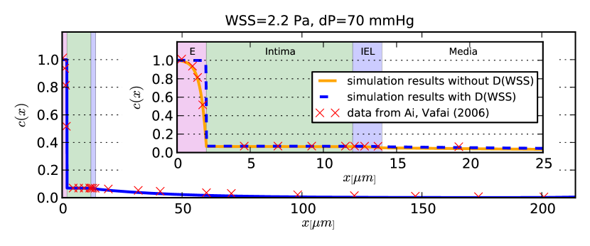
Figure 3: LDL concentration profile in the arterial wall normalized to the input concentration $C_{0}$. $x$ is the distance from the lumen. Comparison with the results from the work of Ai, Vafai 2006. The blue dashed line shows the simulation results for the parameters (4LA) from the Table 1 and the orange continuous line shows the simulation results for the parameters (4LA) with the endothelium diffusion coefficient independent on WSS, but get from [7] equal to $8.15\times 10^{-11}mm^{2}/s$. The red crosses show the data from the work [7]. Simulation parameters: $dP=70\mathrm{mmHg}$, $\mathrm{WSS}=2.2$ Pa. The individual layers are marked with colors: magenta is endothelium, green is intima, blue is IEL and white is media. Inset graph is an enlargement of the area from $0\mu m$ to $25\mu m$.

In the Figure 4 a comparison of the results for (4LC) parameters listed in the Table 2 with results from [8] is shown. In this case there is no difference in the endothelium LDL profile. Based on it, it can be assumed that the dependence $D(\mathrm{WSS})$ from Equation 10 correctly reproduces the endothelium diffusion coefficient in function of the WSS.

To sum up, in the case of high WSS that two sets of parameters give similar LDL concentration profiles. In this case relationship, known from the literature, for example from the single-layer model shown in [9] is visible. The concentration of LDL in the intima is at the level of one order of magnitude lower then input concentration (the value depends on the used set of parameters).

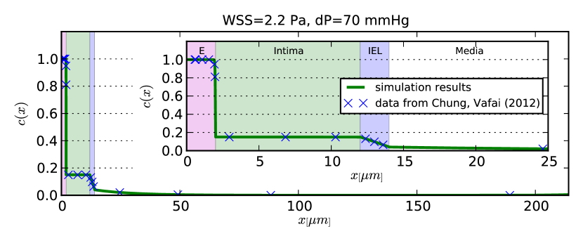
Figure 4: LDL concentration profile in the arterial wall normalized to the input concentration $C_{0}$. $x$ is the distance from the lumen. Comparison with the results from the work of Chung, Vafai 2012 [8]. The green line shows the simulation results for the parameters (4LC) from the Table 2. Cyan crosses shows data from [8]. Simulation parameters: $dP=70mmHg$, $\mathrm{WSS}=2.2Pa$. The individual layers are marked with colors: magenta is endothelium, green is intima, blue is IEL and white is media. Inset graph is an enlargement of the area from $0\mu m$ to $25\mu m$.

6.2 Giant LDL accumulation effect for low WSS

The most interesting regime is at low WSS values. The low wall shear stress is present near stagnation points. It can lead to enhanced penetration of LDL which further is a cause for plague formation in the arterial wall.

The main barrier in LDL transport at normal physiological conditions (high WSS) is the endothelium. On the other hand IEL layer has filtration reflectivity significantly larger than the coefficients of adjacent layers: the intima and media. If the low WSS influence would significantly increase transport of LDL through the endothelium, then it could lead to the accumulation of LDL by the IEL layer.

Indeed, this effect can be observed. In Figure 5 we take very small value of $WSS=0.02Pa$. The dramatic difference to the high WSS case is very high level of LDL in the intima. Depending on the choice of parameters it can even few times exceed the value of the LDL concentration in the lumen. Note, that this effect is not possible in the single-layer model.

The effect of the LDL accumulation in the intima is clearly visible in the Figure 6, which shows the relationship between WSS and LDL concentration in the intima on the border of the endothelium. Despite of the significant difference between the results for each group of parameters, in both cases the effect of huge LDL accumulation is visible.

In the single-layer model maximum LDL concentration normalized to input $C_{0}$ for the zero WSS is about $0.25$, as shown in the Figure 7. In the four-layer model that relative concentration is $1.0$ or $4.5$, depending on the taken set of parameters, which is $4\times$ - $18\times$ greater than in the single-layer model. It means that the model with internal structure of the arterial wall predicts the LDL concentrations of the order of magnitude larger than single-layer one.

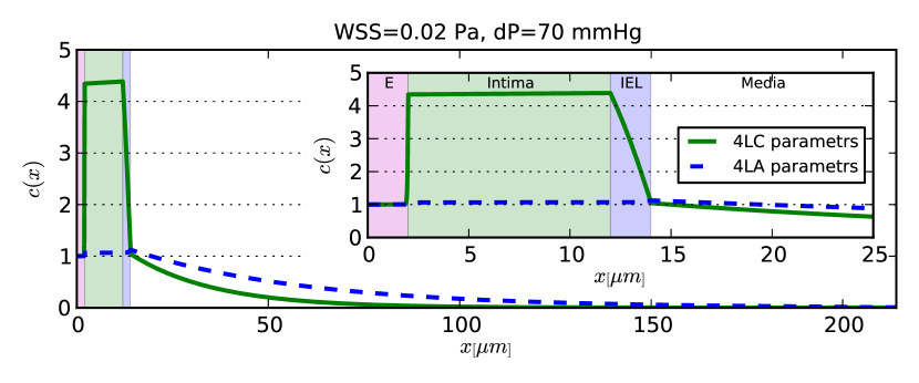
Figure 5: LDL concentration profile in the arterial wall normalized to the input concentration $C_{0}$. $x$ is the distance from the lumen. Green continuous line shows the simulation results for the (4LC) parameters from the Table 2, and the dashed blue line shows the simulation results for the (4LA) parameters from the Table 1. Simulation parameters: $dP=70mmHg$, $WSS=0.02Pa$. The individual layers are marked with colors: magenta is endothelium, green is intima, blue is IEL and white is media. Inset graph is an enlargement of the area from $0\mu m$ to $25\mu m$.

Figure 6: WSS dependence of the intima side LDL concentration at the endothelium. Green continuous line shows the simulation results for the (4LC) parameters from the Table 2, and the blue dashed line shows the simulation results for the (4LA) parameters from the Table 1.

6.3 Properties of two-layer model

We have simplified our LDL transport model to one spatial dimension. While the arguments of scale separation seem to be valid, it can be more convincing to present some direct comparisons.

In the work [9] a single-layer model of blood vessel was used, treating arterial wall as homogeneous layer with endothelium as a boundary condition. Effectively it means that the arterial wall consists of the “zero” length boundary condition representing the endothelium and the layer representing the interior of the wall. Using our algorithm which is based on transport in connected regions with piecewiese constant coefficients, we constructed two-layer model, which effectively corresponds to the single-layer model used by Olgac et al. In this model, endothelium is treated as a separate layer (thin, however nonzero length) modeled in exactly the same way as in the four-layer model with the WSS dependence. The other layer is considered as a homogeneous porous medium (arterial wall) with the parameters from the Olgac work. The parameters are shown in the Table 3.

In the Figure 7 we show an obtained LDL concentration profile in the arterial wall together with the computational results of Olgac et al. from [9] and experimental results of Meyer et al. from [45]. We see that they are essentially the same. Interestingly, the same concentration profile at this WSS can be obtained from four-layer model.

The key element of the modeling in this paper is a WSS influence on the transport. Therefore in Figure 8 we compare the results obtained by Olgac[9] and our models. We see that results coincide perfectly. This ultimately provides the evidence that the simplified, one dimensional modeling can be used in this case. The huge advantage of such simplification is possibility of exploration of the fine structure of the wall with relatively small computational effort. Moreover, the single-layer model cannot predict the effect of giant LDL accumulation.

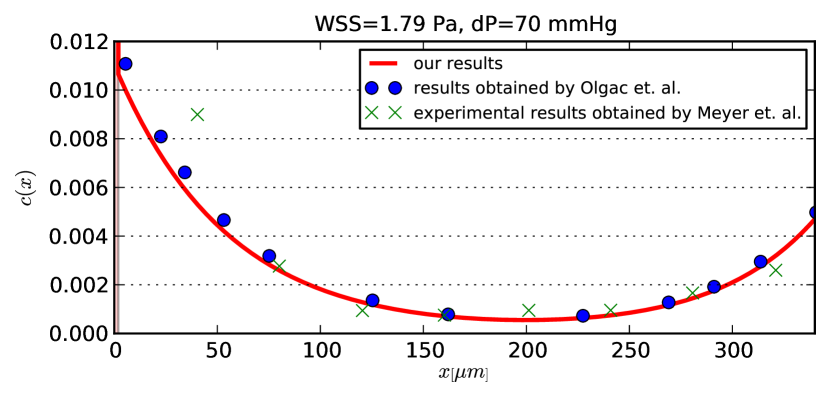
Figure 7: Comparison of the computed solute concentration profile across the artery wall with the experimental results of Meyer et al. [45] signed by green crosses and Olgac et al. [9] marked by blue dots at $dP=70mmHg$ and $WSS=1.79Pa$. $c$ is the arterial wall concentration normalized by the inlet concentration $C_{0}$, and $x$ is the distance from the lumen. The individual layers are marked with colors: red - endothelium and white: rest of arterial wall. In that picture the endothelium layer is almost invisible.

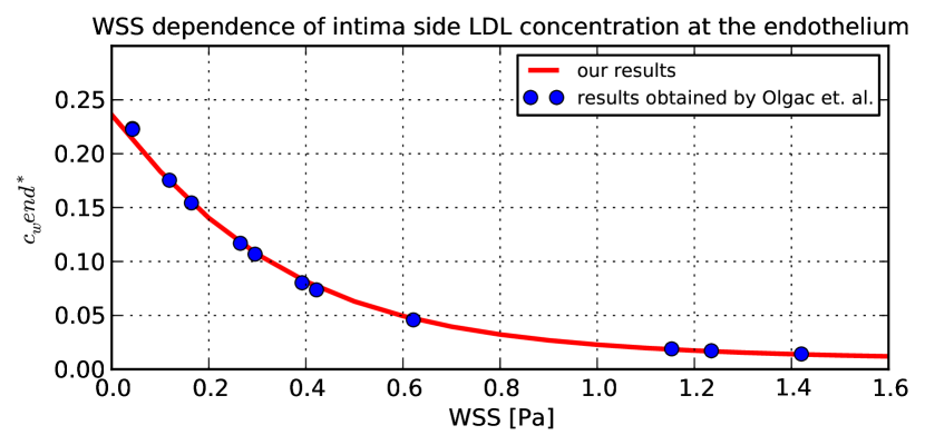
Figure 8: WSS Dependence of intima side LDL concentration at the endothelium. Blue line is our simulation results, green crosses are results obtained from paper Olgac et al. [9]

7 Conclusions

The first and main result of this paper is a demonstration of the giant LDL accumulation in the intima. This effect is related to the layered structure of the artery. In the four-layer model IEL is a significant barrier for LDL macromolecules and for this reason they accumulate in the intima. Our research shows that the LDL concentration can be up to $18$ times larger than predictions from single-layer models. We believe that such giant accumulation can play a significant role in the explanations of the atherosclerosis development.

Additionally we have shown that the full three dimensional simulation of the LDL filtration process gives basically the same result as one dimensional approximation. It can be valuable information for further construction of advanced models, since it make the three dimensional solver redundant.

8 Acknowledgments

K.J. acknowledges a scholarship from the TWING and FORSZT projects co-financed by the European Social Fund.

9 Literature

References

-
[1]
Git repository.
URL https://github.com/marcinofulus/LDLtransport - [2] S. S. Chugh, K. Reinier, C. Teodorescu, A. Evanado, E. Kehr, M. Al Samara, R. Mariani, K. Gunson, J. Jui, Epidemiology of sudden cardiac death: clinical and research implications, Progress in cardiovascular diseases 51 (3) (2008) 213–228.
- [3] M. A. Rosenberg, F. L. Lopez, P. POPRAWIC, S. Adabag, L. Y. Chen, N. Sotoodehnia, R. A. Kronmal, D. S. Siscovick, A. Alonso, A. Buxton, et al., Height and risk of sudden cardiac death: the atherosclerosis risk in communities and cardiovascular health studies, Annals of epidemiology.
- [4] S. S. Chugh, J. Jui, K. Gunson, E. C. Stecker, B. T. John, B. Thompson, N. Ilias, C. Vickers, V. Dogra, M. Daya, et al., Current burden of sudden cardiac death: multiple source surveillance versus retrospective death certificate-based review in a large us community, Journal of the American College of Cardiology 44 (6) (2004) 1268–1275.
- [5] J. M. Tarbell, Mass transport in arteries and the localization of atherosclerosis, Annual review of biomedical engineering 5 (1) (2003) 79–118.
- [6] S. Yiannis, U. Ahmet, J. Michael, et al., Role of endothelial shear stress in the natural history of coronary atherosclerosis and vascular remodeling, J Am Coll Cardiol 49 (2007) 2379–2393.
- [7] L. Ai, K. Vafai, A coupling model for macromolecule transport in a stenosed arterial wall, International Journal of Heat and Mass Transfer 49 (9) (2006) 1568–1591.
- [8] S. Chung, K. Vafai, Effect of the fluid–structure interactions on low-density lipoprotein transport within a multi-layered arterial wall, Journal of biomechanics 45 (2) (2012) 371–381.
- [9] U. Olgac, V. Kurtcuoglu, D. Poulikakos, Computational modeling of coupled blood-wall mass transport of ldl: effects of local wall shear stress, American Journal of Physiology-Heart and Circulatory Physiology 294 (2) (2008) H909–H919.
- [10] C. Michel, F. Curry, Microvascular permeability, Physiological reviews 79 (3) (1999) 703–761.
- [11] N. Yang, K. Vafai, Modeling of low-density lipoprotein (ldl) transport in the artery—effects of hypertension, International Journal of Heat and Mass Transfer 49 (5) (2006) 850–867.
- [12] M. Prosi, P. Zunino, K. Perktold, A. Quarteroni, Mathematical and numerical models for transfer of low-density lipoproteins through the arterial walls: a new methodology for the model set up with applications to the study of disturbed lumenal flow, Journal of biomechanics 38 (4) (2005) 903–917.
- [13] G. Rappitsch, K. Perktold, Pulsatile albumin transport in large arteries: a numerical simulation study, Journal of biomechanical engineering 118 (4) (1996) 511–519.
- [14] S. Wada, T. Karino, Computational study on ldl transfer from flowing blood to arterial walls, in: Clinical Application of Computational Mechanics to the Cardiovascular System, Springer, 2000, pp. 157–173.
- [15] J. Moore, C. Ethier, Oxygen mass transfer calculations in large arteries, Journal of biomechanical engineering 119 (4) (1997) 469–475.
- [16] N. Yang, K. Vafai, Low-density lipoprotein (ldl) transport in an artery–a simplified analytical solution, International Journal of Heat and Mass Transfer 51 (3) (2008) 497–505.
- [17] P. A. VanderLaan, C. A. Reardon, G. S. Getz, Site specificity of atherosclerosis site-selective responses to atherosclerotic modulators, Arteriosclerosis, thrombosis, and vascular biology 24 (1) (2004) 12–22.
- [18] C. Caro, J. Fitz-Gerald, R. Schroter, Arterial wall shear and distribution of early atheroma in man.
- [19] T. Asakura, T. Karino, Flow patterns and spatial distribution of atherosclerotic lesions in human coronary arteries., Circulation research 66 (4) (1990) 1045–1066.
- [20] D. N. Ku, D. P. Giddens, C. K. Zarins, S. Glagov, Pulsatile flow and atherosclerosis in the human carotid bifurcation. positive correlation between plaque location and low oscillating shear stress., Arteriosclerosis, Thrombosis, and Vascular Biology 5 (3) (1985) 293–302.
- [21] J. E. Moore Jr, C. Xu, S. Glagov, C. K. Zarins, D. N. Ku, Fluid wall shear stress measurements in a model of the human abdominal aorta: oscillatory behavior and relationship to atherosclerosis, Atherosclerosis 110 (2) (1994) 225–240.
- [22] J. R. Buchanan Jr, C. Kleinstreuer, G. A. Truskey, M. Lei, Relation between non-uniform hemodynamics and sites of altered permeability and lesion growth at the rabbit aorto-celiac junction, Atherosclerosis 143 (1) (1999) 27–40.
- [23] C. Cheng, R. van Haperen, M. de Waard, L. C. van Damme, D. Tempel, L. Hanemaaijer, G. W. van Cappellen, J. Bos, C. J. Slager, D. J. Duncker, et al., Shear stress affects the intracellular distribution of enos: direct demonstration by a novel in vivo technique, Blood 106 (12) (2005) 3691–3698.
- [24] V. Gambillara, C. Chambaz, G. Montorzi, S. Roy, N. Stergiopulos, P. Silacci, Plaque-prone hemodynamics impair endothelial function in pig carotid arteries, American Journal of Physiology-Heart and Circulatory Physiology 290 (6) (2006) H2320–H2328.
- [25] P. H. Stone, A. U. Coskun, S. Kinlay, M. E. Clark, M. Sonka, A. Wahle, O. J. Ilegbusi, Y. Yeghiazarians, J. J. Popma, J. Orav, et al., Effect of endothelial shear stress on the progression of coronary artery disease, vascular remodeling, and in-stent restenosis in humans in vivo 6-month follow-up study, Circulation 108 (4) (2003) 438–444.
- [26] J. J. Wentzel, R. Krams, J. C. Schuurbiers, J. A. Oomen, J. Kloet, W. J. van der Giessen, P. W. Serruys, C. J. Slager, Relationship between neointimal thickness and shear stress after wallstent implantation in human coronary arteries, Circulation 103 (13) (2001) 1740–1745.
- [27] J. J. Wentzel, R. Corti, Z. A. Fayad, P. Wisdom, F. Macaluso, M. O. Winkelman, V. Fuster, J. J. Badimon, Does shear stress modulate both plaque progression and regression in the thoracic aorta? human study using serial magnetic resonance imaging, Journal of the American College of Cardiology 45 (6) (2005) 846–854.
- [28] A. M. Malek, S. L. Alper, S. Izumo, Hemodynamic shear stress and its role in atherosclerosis, Jama 282 (21) (1999) 2035–2042.
- [29] P. H. Stone, A. U. Coskun, Y. Yeghiazarians, S. Kinlay, J. J. Popma, R. E. Kuntz, C. L. Feldman, Prediction of sites of coronary atherosclerosis progression: in vivo profiling of endothelial shear stress, lumen, and outer vessel wall characteristics to predict vascular behavior, Current opinion in cardiology 18 (6) (2003) 458–470.
- [30] M. A. Gimbrone, J. N. Topper, T. Nagel, K. R. Anderson, G. GARCIA-CARDEÑA, Endothelial dysfunction, hemodynamic forces, and atherogenesisa, Annals of the New York Academy of Sciences 902 (1) (2000) 230–240.
- [31] S. Dimmeler, J. Haendeler, V. Rippmann, M. Nehls, A. M. Zeiher, Shear stress inhibits apoptosis of human endothelial cells, FEBS letters 399 (1) (1996) 71–74.
- [32] T. Frauenfelder, E. Boutsianis, T. Schertler, L. Husmann, S. Leschka, D. Poulikakos, B. Marincek, H. Alkadhi, Flow and wall shear stress in end-to-side and side-to-side anastomosis of venous coronary artery bypass grafts, Biomedical engineering online 6 (1) (2007) 35.
- [33] M. Dabagh, P. Jalali, J. M. Tarbell, The transport of ldl across the deformable arterial wall: the effect of endothelial cell turnover and intimal deformation under hypertension, American Journal of Physiology-Heart and Circulatory Physiology 297 (3) (2009) H983.
- [34] Y. Huang, D. Rumschitzki, S. Chien, S. Weinbaum, A fiber matrix model for the growth of macromolecular leakage spots in the arterial intima, Journal of biomechanical engineering 116 (4) (1994) 430–445.
- [35] A. Suciu, Effects of external forces on endothelial cells, Ph.D. thesis, Lausanne (1997). doi:10.5075/epfl-thesis-1614.
- [36] J.-J. Chiu, D. Wang, S. Chien, R. Skalak, S. Usami, Effects of disturbed flow on endothelial cells, Journal of biomechanical engineering 120 (1) (1998) 2–8.
- [37] N. Sakamoto, T. Ohashi, M. Sato, Effect of shear stress on permeability of vascular endothelial monolayer cocultured with smooth muscle cells, JSME International Journal Series C 47 (4) (2004) 992–999.
- [38] S. Chien, Molecular and mechanical bases of focal lipid accumulation in arterial wall, Progress in biophysics and molecular biology 83 (2) (2003) 131–151.
- [39] S.-J. Lin, K.-M. Jan, S. Weinbaum, S. Chien, Transendothelial transport of low density lipoprotein in association with cell mitosis in rat aorta., Arteriosclerosis, Thrombosis, and Vascular Biology 9 (2) (1989) 230–236.
- [40] C. Michel, F. Curry, Microvascular permeability, Physiological reviews 79 (3) (1999) 703–761.
- [41] C. S. Patlak, S. I. Rapoport, Theoretical analysis of net tracer flux due to volume circulation in a membrane with pores of different sizes relation to solute drag model, The Journal of general physiology 57 (2) (1971) 113–124.
- [42] B. Rippe, B. Haraldsson, Transport of macromolecules across microvascular walls: the two-pore theory, Physiological reviews 74 (1) (1994) 163–219.
- [43] M. R. Kellen, J. B. Bassingthwaighte, Transient transcapillary exchange of water driven by osmotic forces in the heart, American Journal of Physiology-Heart and Circulatory Physiology 285 (3) (2003) H1317–H1331.
- [44] V. Silva, P. Prádanos, L. Palacio, A. Hernández, Alternative pore hindrance factors: What one should be used for nanofiltration modelization?, Desalination 245 (1) (2009) 606–613.
- [45] G. Meyer, A. Tedgui, et al., Effects of pressure-induced stretch and convection on low-density lipoprotein and albumin uptake in the rabbit aortic wall, Circulation research 79 (3) (1996) 532–540.